Integrating Point Process Models, Evolutionary Ecology and Traditional Knowledge Improves Landscape Archaeology—A Case from Southwest Madagascar

Abstract

Landscape archaeology has a long history of using predictive models to improve our knowledge of extant archaeological features around the world. Important advancements in spatial statistics, however, have been slow to enter archaeological predictive modeling. Point process models (PPMs), in particular, offer a powerful solution to explicitly model both first- and second-order properties of a point pattern. Here, we use PPMs to refine a recently developed remote sensing-based predictive algorithm applied to the archaeological record of Madagascar’s southwestern coast. This initial remote sensing model resulted in an 80% true positive rate, rapidly expanding our understanding of the archaeological record of this region. Despite the model’s success rate, it yielded a substantial number (~20%) of false positive results. In this paper, we develop a series of PPMs to improve the accuracy of this model in predicting the location of archaeological deposits in southwest Madagascar. We illustrate how PPMs, traditional ecological knowledge, remote sensing, and fieldwork can be used iteratively to improve the accuracy of predictive models and enhance interpretations of the archaeological record. We use an explicit behavioral ecology theoretical framework to formulate and test hypotheses utilizing spatial modeling methods. Our modeling process can be replicated by archaeologists around the world to assist in fieldwork logistics and planning.

1. Introduction

Predictive modeling has been a staple of landscape-scale archaeological investigations for decades [1,2,3,4,5,6]. These models are critical not only for the identification of archaeological features but also for understanding the processes underlying their distributional patterns. The methods employed for the development of predictive models in archaeology are varied and often integrate expert knowledge, geographic information systems (GIS), remote sensing analysis [2,7,8], linear regression [9,10,11,12], and other approaches (see References [6,13]). Other spatial statistical methods can also be used for developing such models, but, to-date, have been underutilized in archaeology. Predictive modeling in archaeology is also often limited by the lack of explicit theoretical frameworks to interpret patterns in the archaeological record [6,14]. As we demonstrate below, the integration of theory from human behavioral ecology (HBE) into predictive models allows us to test hypotheses about processes driving human settlement on a landscape and improve our interpretations of settlement patterns.

One example of an underutilized statistical method is point process modeling. Point processes are the mechanisms that produce a point pattern (i.e., spatial distribution of points). Point process models (PPMs) represent a large class of spatially-explicit models that are used to evaluate the underlying processes responsible for different properties of spatial patterns (see Reference [15]). A core strength of point process modeling is the ability to characterize and distinguish between the effects of the first- and second-order properties of a point process.

A fundamental principle of point pattern analysis is the distinction between the first- and second-order properties of spatial point processes (for a detailed discussion see ref [16] (pp. 41–43)). The first-order property is the intensity of the underlying process and refers to variability in the density of points across a study region. The intensity includes both the average number of points per unit area and the degree to which density varies with location, which can be spatially variable (i.e., an inhomogeneous process) or constant within a given region (i.e., homogenous process) [15]. On a landscape, the first-order intensity of a point pattern often results from a relationship between the density of a class of points and external variables. For example, freshwater (external variable) may influence the distribution of archaeological materials (class of points) on a landscape, such as increased settlement density near freshwater sources, or the density of trees (class of points) may be influenced by changes in altitude (external variable).

The second-order property is the interaction or dependence between points in a point pattern, which results from a process whereby points influence the locations of other points. This second-order property is typically characterized by different degrees of clustering or dispersion. In human settlements, for example, second-order properties can consist of processes related to population interaction (e.g., social or kinship networks, conflict, territoriality, etc.) that might result in different degrees of settlement nucleation or spacing. As first- and second-order properties are distinct and result from different kinds of processes, distinguishing between these two properties is a major focus of point pattern analysis that is critical for accurately modeling and explaining spatial processes [15,16,17,18].

For instance, it is possible that a first-order trend may be mistaken for second-order interaction simply because points have spatially varying density. In human settlements, for example, we might confuse a first-order trend, such as higher density near water sources, for second-order settlement clustering, when in fact the pattern may be sufficiently accounted for by the first-order effect. It is also possible for a model to under account for settlement clustering or dispersion by not including a second-order interaction component. Thus, attempting to account for the effects of both first- and second-order interaction should be a primary concern in settlement pattern analyses [17,19,20]. PPMs offer a range of statistical tools to better investigate the relative importance of different factors responsible for spatial patterns in the archaeological record, including second-order properties. Thus, PPMs can allow archaeologists to distinguish between first- and second-order effects in settlement patterns even when data on social interaction remain unknown or poorly understood. This is critical particularly in areas where archaeological investigation is still nascent. While the use of PPMs in archaeology as explanatory tools has increased in recent years [17,19,21,22,23,24,25,26,27,28,29,30,31], they are still relatively underutilized and few studies have explicitly used them for predictive modeling of site distributions [32].

In what follows, we employ and assess the efficacy of PPMs for iteratively refining predictive models for archaeological survey, using southwest Madagascar as a case study. Madagascar is the fourth largest island on Earth and contains a vast archaeological record, but areal coverage through survey or excavation remain limited in many parts of the island. The region is also important for understanding human history, as it sits at the crossroads of a number of major migration routes and trade networks in the Indian Ocean [33,34,35,36]. Despite decades of research, however, there is still significant debate about the timing and nature of the island’s initial settlement by people and the subsequent expansion of settlements across the island [37,38,39,40].

In southwest Madagascar, communities traditionally practice a mixed economy consisting of foraging, fishing, herding, and farming [41,42,43,44,45]. Cultural identity in the region is tied to ancestral clan affiliation as well as to dominant subsistence practices [44]. The coastal region is occupied by Vezo (who are primarily fishers), Masikoro (who are primarily agropastoralists), and Mikea (who primarily occupy and forage in the dry forests further inland) [43,44]. While there is evidence that foraging populations have lived on Madagascar for thousands of years [38,40,46], the exact timing of human arrival in the southwest and elsewhere on the island is still subject to intense debate among archaeologists [37,39]. 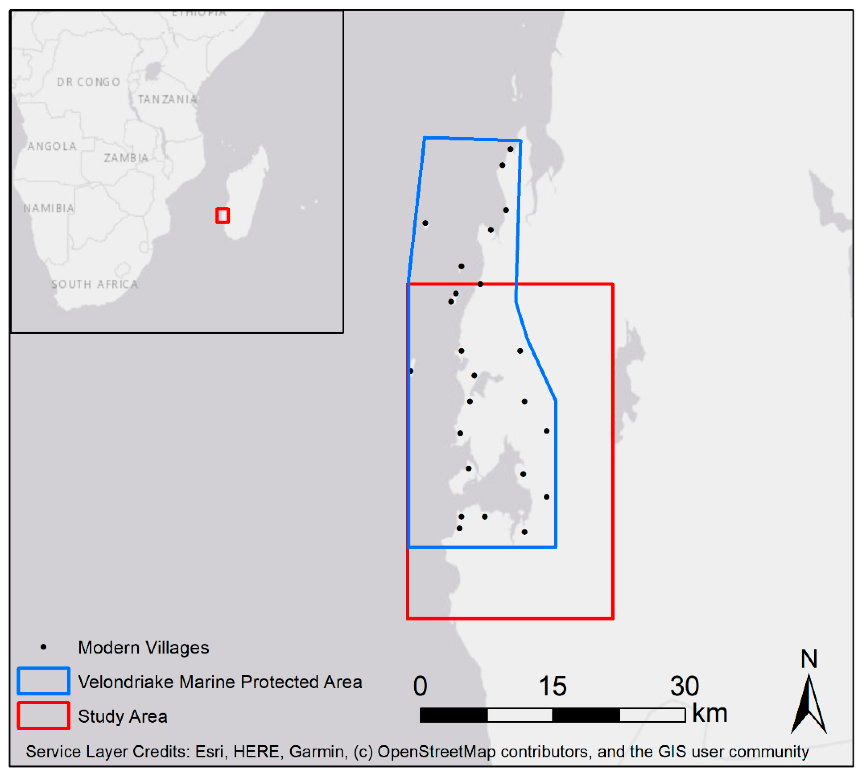Based upon limited evidence, it is likely that these early human populations were small foraging communities that occupied areas around river valleys [47] and karst landscapes along the island’s coasts [46,48]. To better understand settlement patterns on the southwest coast, Davis and colleagues [49] developed an HBE-based remote sensing/GIS predictive model for locating Late Holocene archaeological deposits in coastal southwestern Madagascar and interpreting their distribution (Figure 1).

The model developed by Davis et al. [49] is rooted in HBE, specifically the ideal-free distribution (IFD) model, which assumes that the greatest overall habitat suitability (measured by the availability of important environmental resources) will reflect where a population will preferentially choose to settle [50,51,52]. Using the theoretical predictions of an IFD (i.e., communities will first choose to settle the most suitable habitats, identified on the basis of resource availability, followed by lower suitability regions) the team compiled a list of important ecological variables, which were recorded in ethnohistoric records [53]. The invaluable insight provided by such traditional ecological knowledge (TEK) has been well established [54,55,56]. In particular, TEK has increased archaeology’s ability to inform the present by tracing feedback loops between human behavior and environmental change [57,58]. Davis and colleagues [49] then digitized these features using satellite imagery and automated image analysis procedures and developed a predictive model rooted in the assumption that the closer a point on the landscape is to these resources, the higher the likelihood of people settling these locations. During ground testing of the algorithm, more than 1000 individual artifacts were recovered from 74 locations throughout the study area in southwest Madagascar, with most of these materials coming from locations ranked as having a “high probability” of containing archaeological deposits.

Nonetheless, in 20% of instances, the predictive model ranked an area as “high probability” where no archaeological materials were recorded during pedestrian survey. The occurrence of false positives leaves room for improvement in the development of the model and also challenges the starting theoretical assumptions of IFD that framed the model. One overlooked factor is that these false positives may result from the omission of important variables in the construction of the model. Another possibility is that certain resources are more important to populations in this area than others, meaning that a uniformly weighted model may not fit as well as a model where some variables are more highly ranked. Site preservation in this region is quite poor and so false positives could also be related to the disappearance of archaeological sites or visibility issues due to dense vegetation (especially in regions further inland). It is also possible that second-order properties (e.g., settlement nucleation or spacing) are leading to greater densities of archaeological material in some areas of high probability but not in others, which suggests that first-order trends do not fully account for spatial patterns on this landscape. This would support the possibility raised by Davis et al. [49] of an Allee-effect, or positive density dependence (a second-order property), on the distribution of sites, whereby areas with mid-level suitability will attract greater population densities because of habitat modifications and community aggregation [51,59,60]. Such community aggregation in lower-suitability environments can also be caused by territoriality, as predicted by the ideal despotic distribution (IDD) model (another model centered on second-order properties) [51,61,62,63]. Allee-effects and IDDs will result in second-order properties (i.e., clustering) not accounted for by a first-order trend and can be characterized with PPMs.

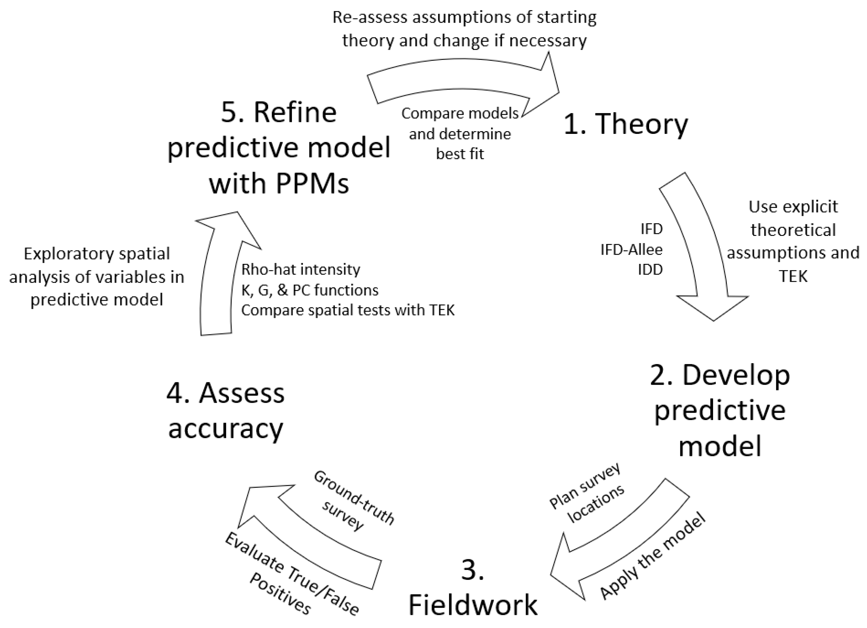
By iteratively developing and evaluating different models, we can improve their accuracy and be better positioned to explain emerging patterns in the archaeological record (Figure 2). In this article, we demonstrate how archaeologists can test the importance of different factors in a model for accurately predicting the location of archaeological deposits. This process allows us to improve the Davis et al. [49] predictive model to increase the number of true positive detections while limiting false positives when directing field surveys.

Building on this previous work by incorporating PPMs allows us to refine the current predictive algorithm for Madagascar and improve its utility for future archaeological investigations. In particular, we demonstrate how PPMs can be used to characterize different environmental variables that predict the first-order intensity of archaeological deposits and also to what degree second-order clustering or dispersion properties improve predictive accuracy. This approach thus aids in understanding the relative importance of different variables and processes responsible for spatial patterns in the archaeological record.

2. Materials and Methods

To re-evaluate the Davis et al. [49] predictive model, we take the previous set of variables incorporated into this model as well as new variables that were previously excluded (

Table 1. List of different variables incorporated in Davis et al. [49] and the models developed in this paper.

Variable	Davis et al. [49]	This Study
Vegetative Productivity	Yes	Yes
Coral Reefs	Yes	Yes
Offshore Islands	Yes	Yes
Distance to the Ocean	Yes	Yes
Paleodunes	Yes	Yes
Rocky outcrops	No	Yes
Depth to bedrock	No	Yes

). The environmental variables used by Davis et al. [49] were generated via automated remote sensing analysis and vegetative index calculations. The same data are used here and are freely available from the Davis et al. [49] publication’s supplemental documents (see https://0-doi-org.brum.beds.ac.uk/10.26207/1a47-pw11).

The Davis et al. [49] algorithm considered the distance from any given point on the landscape to vegetatively productive regions (quantified via soil adjusted vegetation index (SAVI) values [64]), paleodune features (where many recorded archaeological sites in this area are located), offshore islands (which were important refuges from warfare and banditry, as well as important fishing grounds) and coral reefs. In addition to these variables, field observations indicate that rocky outcrops along much of the coastline appear associated with the presence of archaeological deposits. This is potentially related to freshwater access [65] as well as defense and survival strategies. Oral histories from coastal dwelling Vezo communities in the southwest of Madagascar indicate that limestone outcrops often provide good locations for hiding from marauders [66]. Ethnographic and archaeological sources also suggest that freshwater availability is particularly important when selecting village locations [34,42,45,66,67]. The outcrops act as rainwater reservoirs and are still used by communities in the region today for gathering freshwater. Because freshwater source data is not available for the study region, we also use depth to bedrock as a proxy [68,69]. The shallower the bedrock depth, the closer to the surface and more accessible groundwater reservoirs are expected to be. Depth to bedrock and soil data used for our analysis [70] are freely available from the International Soil Reference and Information Centre (ISRIC) Data Hub (https://data.isric.org/geonetwork/srv/eng/catalog.search#/home). While groundwater hydrology is far more complicated than a metric of depth to bedrock [69,71,72], shallow bedrock has been the source of water exploitation for populations in other parts of the world [68,73]. The geology of southwest Madagascar is largely sedimentary, with geologically recent deposits comprised of limestone, sand and other alluvial soils [74,75].

In order to evaluate the overall importance of first and second-order properties (e.g., Allee effect clustering on the archaeological record, as suggested by Davis et al. [49]), we use exploratory point pattern analyses and then build a series of PPMs. Archaeological survey data collected over the past several years by the Morombe Archaeological Project (MAP) [76] are used as the basis of knowledge about the archaeological record. Archaeological points were recorded as artifact clusters (comprised of a mix of materials including ceramic sherds, marine shell tools, faunal remains, and charcoal) during survey of the Davis et al. [49] model and thus each point can represent multiple artifacts at a given location. If some data points represent a single artifact while others represent multiple artifacts, density calculations and the overall intensity of the point pattern can be affected. To ensure that spatial tests are not being skewed due to this fact, we ran all spatial tests twice, once by incorporating the total number of materials as a spatial weight and once without weighting, to see if artifact counts had any spatial effects on the point pattern. Survey locations were chosen using a stratified random strategy and surveyors were not given information about the model’s predictions of site locations, in order to avoid survey bias.

2.1. Point Process Modeling for First-Order Properties

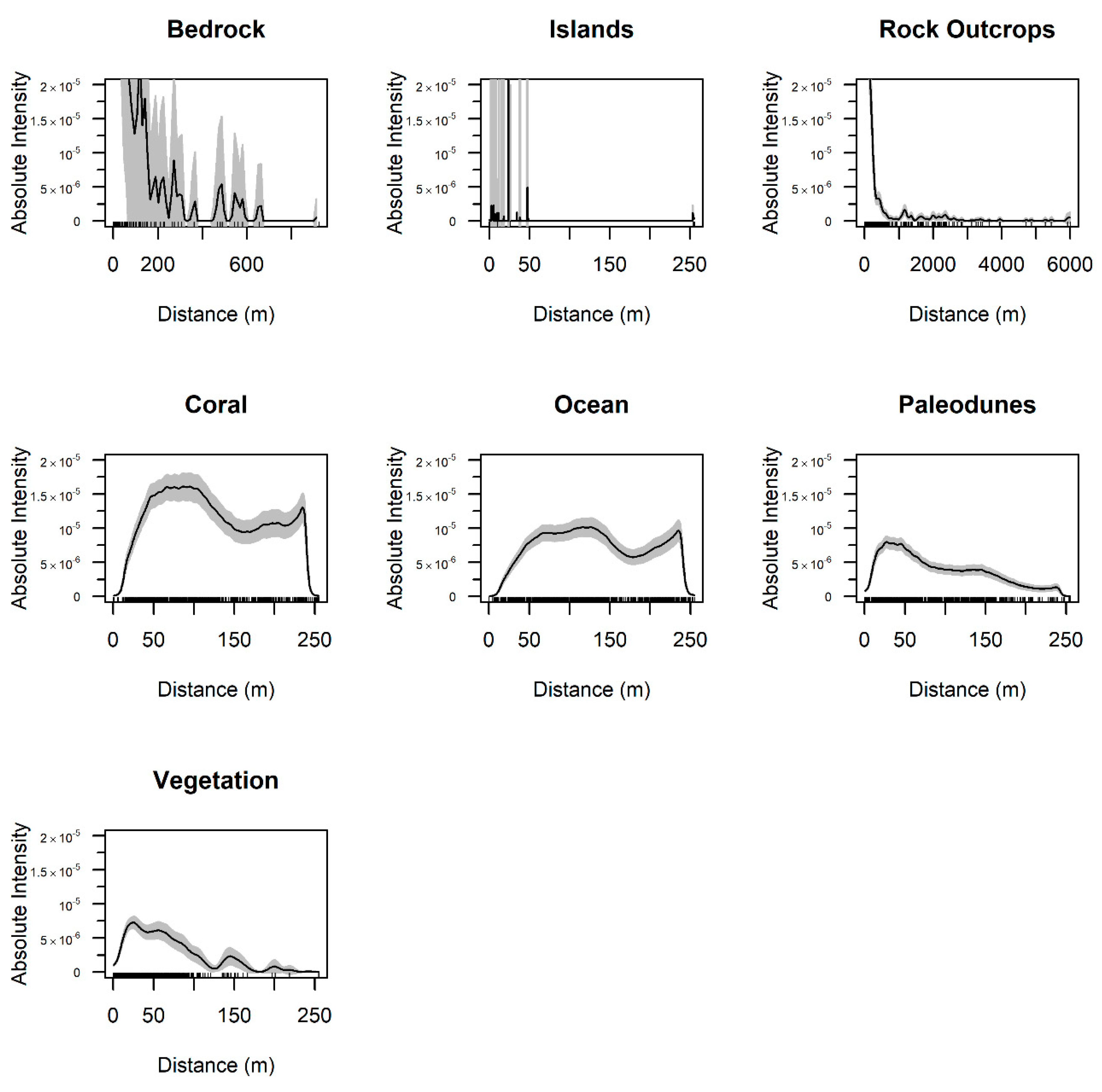
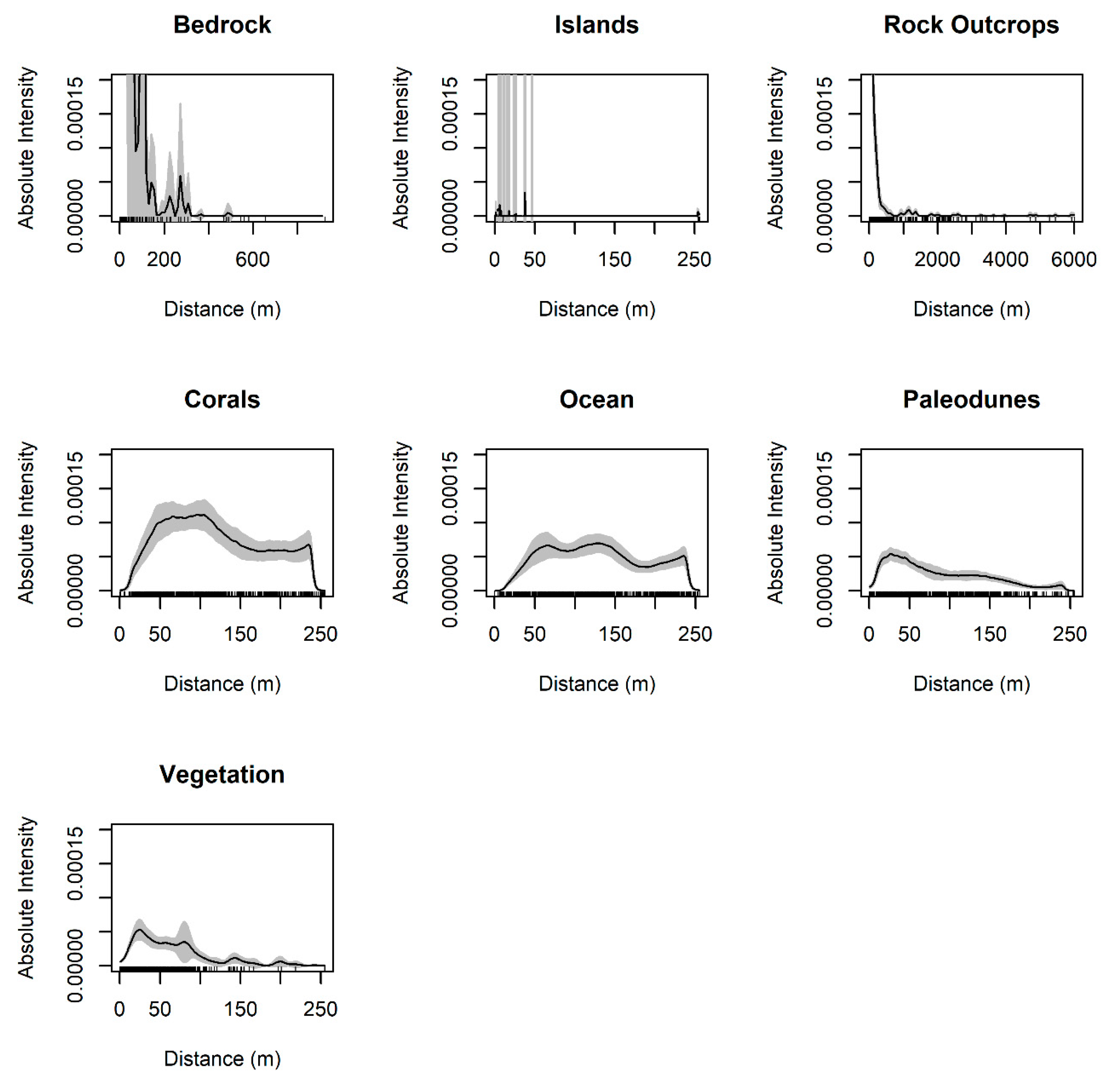
First, we explore first-order trends between the intensity of archaeological deposits in our study area and different covariates (i.e., environmental variables) using nonparametric smoothing (rho-hat function in the spatstat package) [15]. The rho-hat function plots the intensity of a point pattern as a function of a given covariate [15]. In other words, the rho-hat function quantifies the degree to which the density of archaeological deposits is related to a specific variable (e.g., how archaeological deposits are accounted for by vegetation).

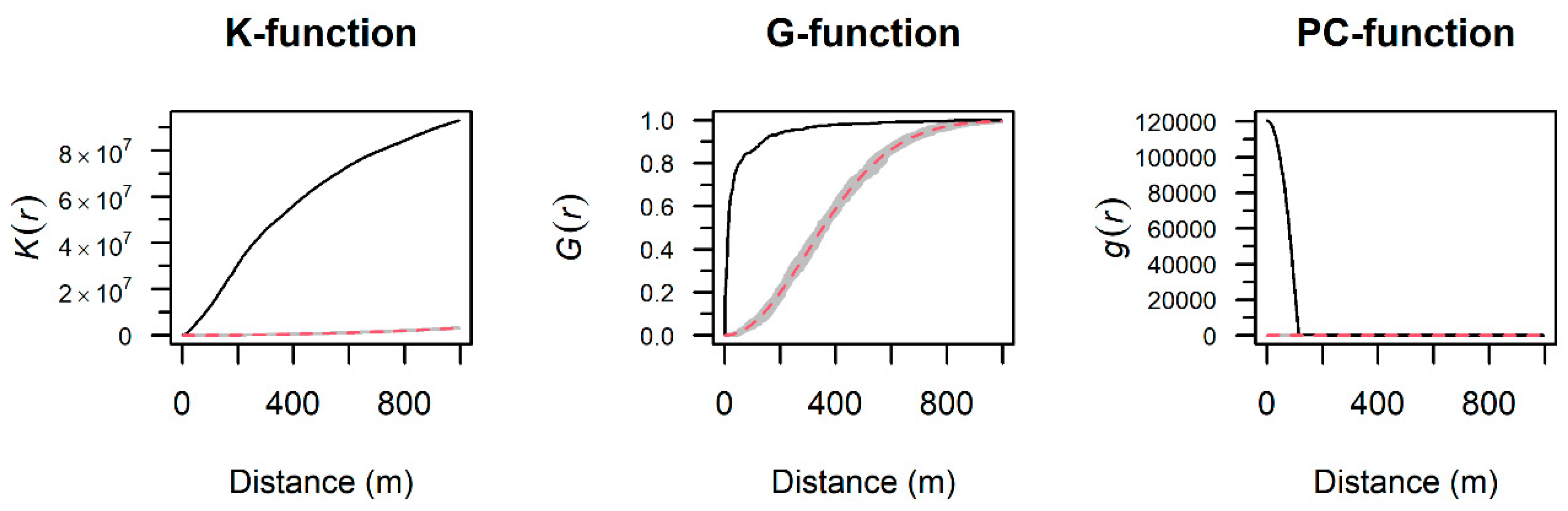
Next, we investigate whether the settlement pattern in our study area exhibits significant degrees of clustering or dispersion (i.e., second-order interactions) by performing K-, G- and pair correlation (PC) function tests on the archaeological point pattern. Each of these summary functions assesses the degree of clustering or dispersion in a point pattern but are somewhat distinct. The K-function [77] calculates the average number of points within a specified radius and is standardized by the intensity of those points (i.e., the number of points is divided by the total area encompassed by point locations). The G-function calculates nearest neighbor distance distribution values for each data point [15]. The PC function assesses whether a point-pattern is significantly more clustered or dispersed than expected for a random pattern but is not cumulative like the other functions [15,78]. The significance of potential clustering or dispersion is assessed by comparing the empirical archaeological patterns to simulated realizations of a random null model. We assess the significance of second-order interaction in these functions using simulation envelopes of a null model of complete spatial randomness (CSR) with 39 Monte Carlo iterations (equivalent to p = 0.05). Significant clustering is inferred when the empirical function (i.e., the archaeological point pattern) is above the simulation envelope. Likewise, significant dispersion between points is inferred when the empirical function is below the simulation envelope. Areas of the empirical function within the envelope are consistent with CSR (i.e., not significantly different from a random pattern).

Following these exploratory analyses of first- and second-order properties we develop a series of PPMs, following similar recent applications [17,20,22]. Our initial PPMs focus on modeling first-order trends and consist of: a homogenous Poisson model (which models the archaeological point pattern as a random process (i.e., CSR)) and two inhomogeneous Poisson models (which model the point pattern as a function of environmental covariates): the Davis et al. [49] model and a new model combining all of the assessed environmental variables (see Table 1). We identify the best fitting model for the settlement pattern using multi-model selection tools, specifically the Akaike Information Criterion (AIC) and Bayesian Information Criterion (BIC) [79,80,81] and a stepwise selection procedure. These model selection tools evaluate how well a statistical model fits a dataset given a tradeoff between model fit and overall complexity of the data [80]. The lower the difference in information criteria score (e.g., ΔAIC and ΔBIC) and the higher the weight (W_i), the better the model. Stepwise selection determines the best fitting model by evaluating how each covariate affects the fit of the overall model and dropping covariates if they result in a higher AIC or BIC score [82].

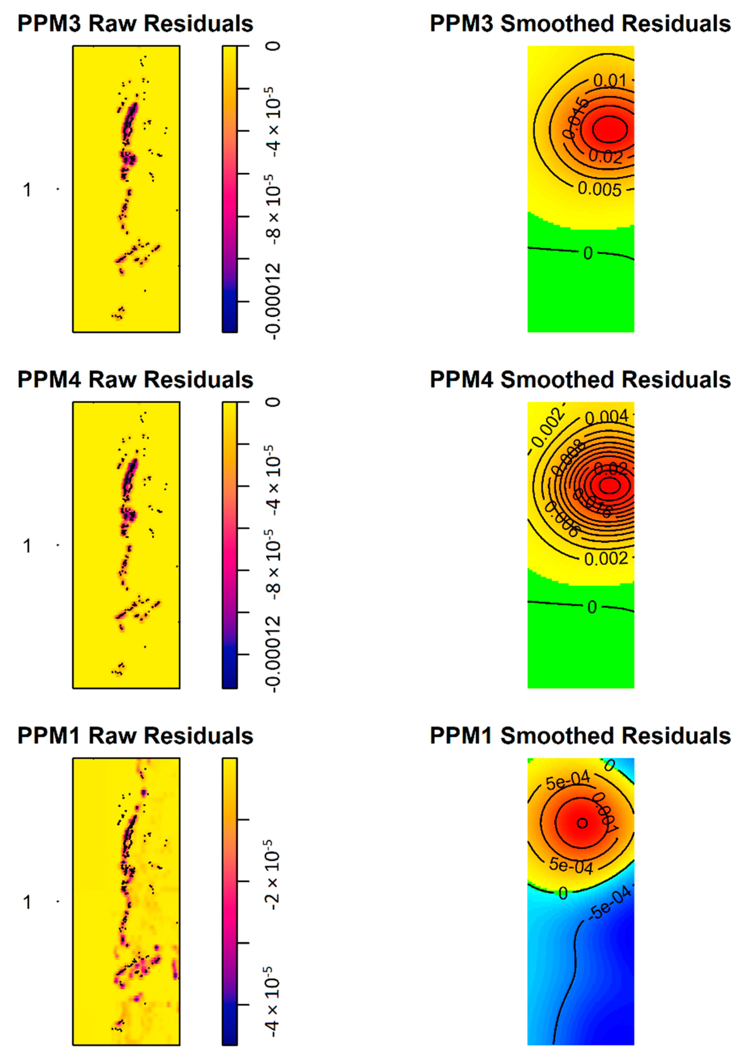
We assess the fit between the best-fitting models and the empirical data in multiple ways. We first evaluate the fit by calculating the raw and kernel-smoothed residual values of our best fitting model and the original Davis et al. [49] model to quantify any deviations between the first-order trend of the fitted model and the empirical data. In other words, the residuals illustrate the goodness-of-fit between the actual locations of archaeological deposits and the locations predicted by the PPM. 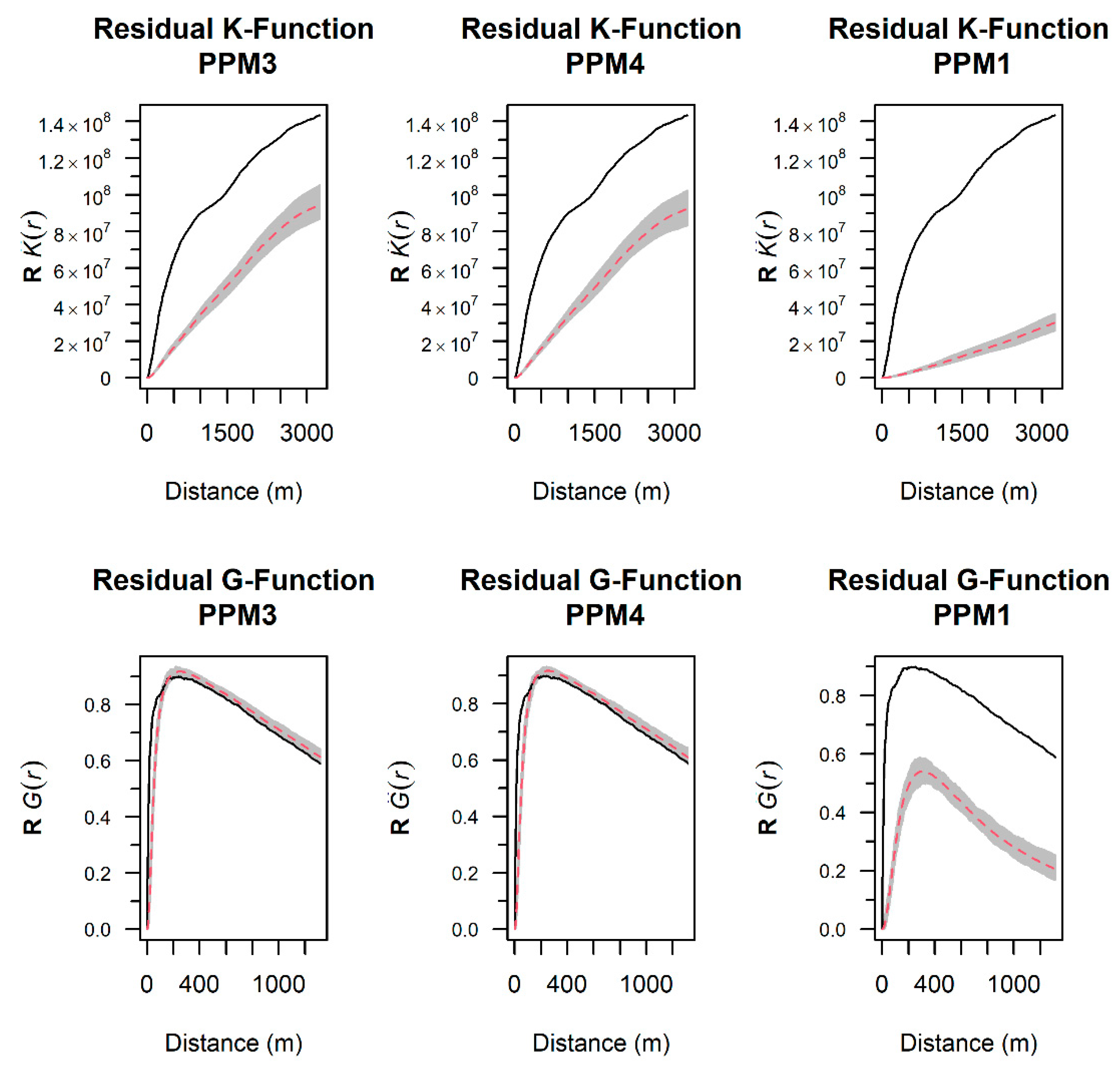Raw residuals estimate the bias within a model and kernel-smoothed residuals use a geographically weighted average of the residuals to account for spatial variance in the raw residual values [83]. We then evaluate the second-order component of the best-fitting models using residual-K and G-functions. These functions assess the fit between the second-order component PPM and the empirical point pattern (i.e., archaeological material distributions) by comparing their K- and G-function estimates with a “compensator,” which is an estimate of the mean value of the K- or G-function [84]. In simpler terms, residual K- and G-functions assess the goodness-of-fit between the predictions of a PPM and the archaeological data in terms of their interpoint relationships (i.e., clustering or dispersion between archaeological points). If the PPM is a good fit to the data, the residual-K and G-functions should lie within the simulation envelope. If the empirical function lies above or below the simulation envelope, this suggests that the empirical pattern is more clustered or dispersed than is accounted for in the model, respectively. In such cases of poor second-order fit, we can improve the models by explicitly including a second-order interaction clustering or dispersion parameter.

2.2. GIS Analysis

Next, using the model selection results of the best-fitting inhomogeneous model, we generate rasterized probability maps (i.e., a series of pixel values situated in geographic space that contain probability values) of places where archaeological sites are expected in ArcGIS 10.7 [85]. Using raster maps, we evaluate the probability scores of different regions within the study area directly with locations of identified archaeological deposits. These maps, in turn, can be used to direct further ground surveys in Madagascar. We create different probability maps by assigning differential weights to each covariate in order of their relative importance. We determine differential weighted values for each covariate based on the rho-hat intensity functions and coefficient estimates from the best-fitting PPM. The greater the intensity measurement and the stronger the coefficient estimates, the greater that covariate’s effect on the archaeological point distribution. By evaluating the difference in intensity and coefficient estimates associated with each covariate we can establish orders of magnitude by which each covariate influences the resulting archaeological point pattern. These values can then be translated into associated rankings (or weights) for each variable.

For example, in this study we are concerned with the relationship of covariates that explain intensities of archaeological deposits at different distances. As such, if we look at three different variables (A, B and C) we can examine: (1) whether all three variables are negatively or positively correlated with archaeological points (i.e., as distance from each variable increases, does the number of archaeological materials decrease or increase, respectively) based on coefficient estimates; and (2) the intensity values of the archaeological points that each variable accounts for based on the rho-hat function and fitted values of the model coefficients. For example, if variable A has a negative relationship with the archaeological point pattern that is three times as strong as variable B and B is twice as negatively related with C, we can use this information as a guide to which variables are most important. Following evaluation of the fitted coefficients, if variable A accounts for 3-times the intensity of a point pattern at small-distances than B, and B accounts for 2-times the intensity of C, we can weight (or rank) variable A at three times that of B and B at twice that of C.

We create different weighted rasters using the raster calculator tool in ArcGIS. Following the creation of these probability rasters, we assess each model by comparing surveyed locations from 2019 (which were used to test the Davis et al. [49] model) with the probability values assigned by the model. If archaeological deposits are recorded in areas that were not predicted (or had low probability values) this indicates a poor fit for that predictive model. In contrast, if deposits are recorded in areas with high probability values, this indicates a better-fitting predictive model. The GIS analysis can be performed in open source platforms as well (e.g., QGIS [86]) and necessary code used for raster calculations is provided in the Supplemental R-markdown document.

Ethnographic data are also incorporated into weighting decisions when explicit information pertaining to the importance of resources is available. For example, ethnohistoric records indicate that coastal Vezo communities in southwest Madagascar place great importance on freshwater availability, access to coral reefs and fisheries, and that rock outcrops have served as a defensive strategy for hiding from foreign invaders [42,43,53,66]. Marine and freshwater resource availability and defensibility of the area are a common rationale for settling an area, and the lack of freshwater or defensibility are most frequently referenced for why people move [53]. As such, results from the prior intensity metrics and coefficient estimates are compared with these ethnographic data and where discrepancies arise (e.g., statistical tests suggest that marine resources are not strongly influencing archaeological points but ethnohistoric records indicate a strong connection), favor is given to the ethnohistoric data. 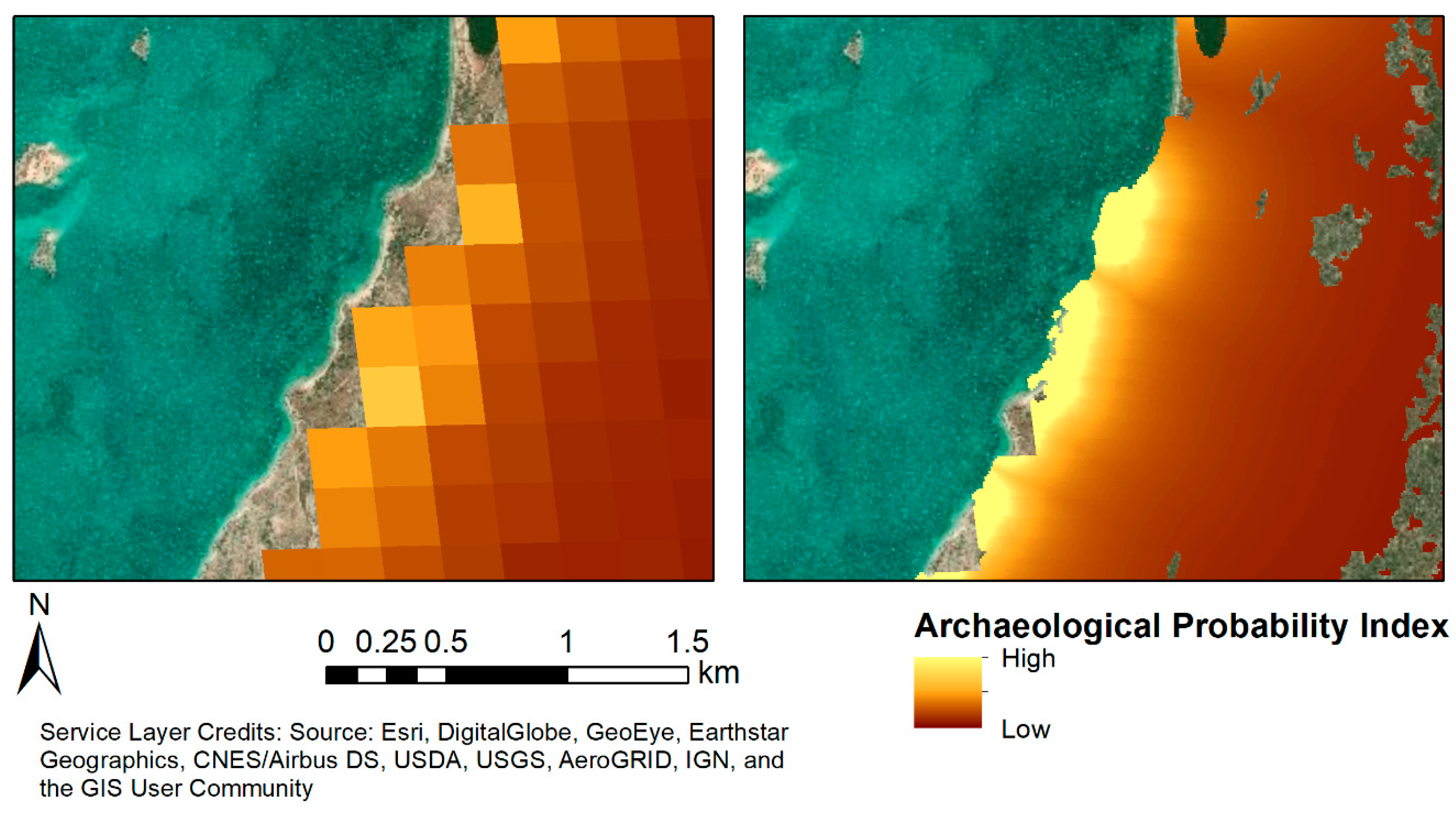Before creating the new probability models in ArcGIS 10.7 [85], the depth to bedrock data is resampled using nearest neighbor interpolation from its original 250m resolution to a resolution of 10m to match the other datasets derived from Sentinel-2 satellite imagery. We resample the dataset iteratively in ArcGIS 10.7 [85] using the resample tool to achieve the best results, from 250 m to 10 m (resampling was conducted four times, first from 250 m to 150 m, second from 150 m to 75 m, third from 75 m to 35 m and fourth from 35 m to 10 m.). When not resampled, the inclusion of this data into raster calculations makes resulting datasets too coarse to direct meaningful ground investigations (Figure 3).

For all models, we take the inverse of the distances from all variables from any given point within the study area (except for bedrock, which is the depth not the distance). This follows Davis et al.’s ([49]) assumption (and the theoretical assumption of IFD) that the closer a point is to these variables the higher the likelihood of human occupation.

Finally, the probability maps are evaluated against each other and the original model published by Davis et al. [49] to determine the most accurate predictive model for archaeological prospection. Accuracy is calculated based on the same 2019 surveys used to ground-truth the original model (see Reference [49]). In all surveyed regions we calculate the probability value assigned by each raster. Because each raster provides only the probability of archaeological materials and not a definitive “yes” or “no” to the presence of cultural deposits, we used a natural breaks method [87] to define “true” or “false” negatives and positives based on the threshold between “high,” “medium” and “low” probability locations. “True positives” are considered as all surveyed locations identified as having “high” likelihood of containing archaeological deposits that did indeed contain artifacts, while “false positives” are all surveyed areas identified as “high” likelihood of containing archaeological materials that did not contain any artifacts. Medium and low likelihood areas are not included in these assessments because the algorithm expects that you might find material but you might not, thus it cannot be counted as a “true” positive or negative. All spatial analyses are conducted in R [88] using the spatstat package [15] and the code is freely available (see Supplemental File). We also use MuMIn [89], maptools [90], raster [91], rgdal [92], rgeos [93], sp [94,95] and MASS [82] packages.

2.3. Point Process Modeling for Second-Order Properties

The best-performing weighted raster and the unweighted raster are imported into R and used to create two PPMs with these rasters as the sole covariates. The unweighted raster created in ArcGIS (representing the best-fitting PPM) is compared against the weighted model, rather than direct comparison with the best fitting PPM to prevent issues in model selection resulting from differences in the number of covariates. A model with six covariates is inherently more complex than a model with one covariate, which can result in higher AIC/BIC scores for the more complex model.

To assess whether the weighted model is a better fit to the data, we compare it with the unweighted PPM using the same multi-model selection approach detailed above [79,80,81]. We then assess second-order interactions by building new models that include an Area Interaction process, which accounts for clustering or dispersion at multiple scales [96]. For these area interaction models, the value of the irregular parameter r is selected by minimizing AIC. We construct three PPMs that add this second-order parameter to the original Davis et al. [49] model, the best-fitting unweighted model, and the best-fitting weighted model. Each of these new PPMs is compared to the other models without second-order properties using multi-model selection. If second-order processes are influencing the archaeological distributional pattern (as predicted by an Allee effect or IDD model), then we expect that the best fitting model will consist of both first-order properties (i.e., environmental variables) and second-order interactions (e.g., clustering).

3. Results

We first present the rho-hat intensity functions, which measure the first-order intensity of archaeological deposits in relation to specific environmental covariates. We examine these patterns using both weighted and unweighted datasets. Figure 4 and Figure 5 show that certain covariates have a greater effect on the intensity of the archaeological point pattern. Specifically, bedrock and rocky outcrops have the strongest negative relationship with the intensity of archaeological points (meaning that intensities are highest at lower distances), while the distance to the ocean, dunes and vegetation values have a weaker negative intensity relationship with archaeological points. These relationships fluctuate, however, as marine resources seem to cycle between increased and decreased intensity over a distance of 250 m. When accounting for the number of artifacts present in each area using a spatial weight, both unweighted (Figure 4) and weighted (Figure 5) results present very similar patterns. This suggests that the effects of different covariates are not strongly influenced by artifact count.

Figure 6 shows the results of K-, G- and PC-functions that test for second-order interactions in the archaeological data. All tests indicate significant clustering between points (p = 0.05). To determine whether spatial intensity is influenced by the amount of material present in a location, we also run these tests using artifact counts as a weighting factor. The results appear identical between weighted and unweighted tests (using artifact counts as a weight), suggesting that population weights are not significantly influencing the results (also see Supplemental File). As such, we proceed with PPMs that weight each point evenly in terms of artifact counts.

3.1. Point Process Modeling of First-Order Properties

Table 2. Results of comparing the different inhomogeneous Poisson point process models using ΔAIC, ΔBIC and their associated weights. PPM3 and PPM4 were the best fitting models according to stepwise model selection using Bayesian Information Criterion (BIC) and Akaike Information Criterion (AIC), respectively. We chose PPM3 (bold text) because it is the simpler of the two models PPM1 (italicized) represents the Davis et al. ([49]) model. Df = degrees of freedom; W_i = information criterion weight value.

Model	Variables	Df	ΔAIC	Wi	ΔBIC	Wi
PPM3	coral, water, islands, rocky shoreline, depth to bedrock	6	1.13	0.256	0	0.848
PPM4	vegetation, coral, water, islands, rocky shoreline, depth to bedrock	7	0	0.452	3.55	0.143
PPM2	vegetation, dunes, coral, water, islands, rocky shoreline, depth to bedrock	8	0.88	0.292	9.12	0.009
PPM1	vegetation, dunes, coral, water, islands	6	3486.97	0	3485.84	0
PPM0	Complete spatial randomness (Poisson Process)	1	6074.78	0	6050.20	0

shows the results of comparing different inhomogeneous Poisson PPMs. The multi-model selection resulted in mixed results, with AIC indicating PPM3 and BIC indicating PPM4 were the best fitting models. The difference between PPM3 and PPM4 is the inclusion of vegetation in PPM4. To decide on the best fitting model, we assessed the relative fit of PPM3 and PPM4 with PPM1 (the original Davis et al. [49] model) using residual plots (Figure 7). We find that PPM3 and PPM4 are very similar and both are better models for archaeological settlement distribution than the Davis et al. [49] model in terms of first-order properties.

Finally, we assess PPM3 and PPM4 with PPM1 in terms of second-order properties using residual K- and G-functions. Figure 8 shows that both PPM3 and PPM4 are negligible in their difference and both perform better (i.e., are a better fit to the archaeological data) than PPM1. Nonetheless, both PPM3 and PPM4 underestimate second-order clustering in the data. As such, we chose PPM3 because it is a simpler model (BIC selection chooses the simplest best performing model), with a ΔAIC = 1.13 and W_i = 0.256 and ΔBIC = 0 and W_i = 0.848.

Table 3. Results of the chosen best fitting model (PPM3), including the parameter estimates and standard errors with a 95% confidence interval for each covariate. S.E. = standard error. CI95 = 95% confidence interval.

	Estimate	S.E.	CI95 Low	CI95 Hi	Ztest	Zval
Intercept	−10.3513	0.24798	−10.8373	−9.865255	<0.0001	−41.7427
Coral	−0.0118	0.00133	−0.014358	−0.0092	<0.0001	−8.8633
Water/Ocean	0.0112	0.001354	0.008508	0.0138	<0.0001	8.2433
Offshore Islands	0.0043	0.000952	0.002429	0.0062	<0.0001	4.5132
Rocky outcrops	−0.0004	0.000061	−0.000504	−0.0003	<0.0001	−6.3179
Depth to Bedrock	−0.0205	0.001075	−0.022596	−0.0184	<0.0001	−19.0557

shows the covariate estimates for PPM3.

3.2. GIS Analysis

We re-create the exact PPM developed in R (PPM3) in ArcGIS, where all variables are evenly weighted. The following formula (1) is used in the raster calculator to create the Unweighted Model:

$$P_{Arch}=\left(\frac{1}{Dpt{h}_{BR}+D_{RO}+D_i+D_C+D_w}\right)$$

(1)

where P_arch = the archaeological probability value, Dpth_BR = depth to bedrock, D_RO = distance to rock outcrops, D_i = distance to offshore islands, D_w = distance to water/ocean, D_c = distance to coral.

Next, we create a predictive raster with weights for each of the variables (see

Table 4. The formulas and respective covariate weights for each predictive model and the results of ground truthed results from the Davis et al. [49] study in relation to each modified algorithm. The best performing model (bolded) produces the most true positives and highest overall values in areas with confirmed archaeological deposits (Table 5). D_v = distance to vegetation (measured by SAVI) and D_d = distance to paleodunes.

Algorithm	Formula	True Positive (#) 1	False Positive (#) 1	# Artifacts (High Prob.)	#Artifacts (Medium Prob.)	# Artifacts (Low Prob.)
Davis et al. [49]	$\frac{1}{{\mathrm{D}}_{\mathrm{V}}+{\mathrm{D}}_{\mathrm{i}}+{\mathrm{D}}_{\mathrm{c}}+{\mathrm{D}}_{\mathrm{w}}+{\mathrm{D}}_{\mathrm{d}}}$	29	7	654	332	141
Unweighted Model	$\frac{1}{{\mathrm{Dpth}}_{\mathrm{BR}}+{\mathrm{D}}_{\mathrm{RO}}+{\mathrm{D}}_{\mathrm{i}}+{\mathrm{D}}_{\mathrm{c}}+{\mathrm{D}}_{\mathrm{W}}}$	28	3	886	102	160
Weighted Model 1	$2.5\left(\frac{1}{{\mathrm{Dpth}}_{\mathrm{BR}}}\right)+2\left(\frac{1}{{\mathrm{D}}_{\mathrm{RO}}}\right)+2\left(\frac{1}{{\mathrm{D}}_{\mathrm{v}}}\right)+1.75\left(\frac{1}{{\mathrm{D}}_{\mathrm{i}}}\right)+1.75\left(\frac{1}{{\mathrm{D}}_{\mathrm{c}}}\right)+1\left(\frac{1}{{\mathrm{D}}_{\mathrm{w}}}\right)+1(\frac{1}{+{\mathrm{D}}_{\mathrm{d}}})$	31	7	955	144	49
Weighted Model 2	$3\left(\frac{1}{{\mathrm{Dpth}}_{\mathrm{BR}}}\right)+2.5\left(\frac{1}{{\mathrm{D}}_{\mathrm{RO}}}\right)+2\left(\frac{1}{{\mathrm{D}}_{\mathrm{v}}}\right)+2\left(\frac{1}{{\mathrm{D}}_{\mathrm{c}}}\right)+1.75\left(\frac{1}{{\mathrm{D}}_{\mathrm{i}}}\right)+1\left(\frac{1}{{\mathrm{D}}_{\mathrm{w}}}\right)+1(\frac{1}{+{\mathrm{D}}_{\mathrm{d}}})$	23	2	813	136	199
Weighted Model 3	$\mathbf{2.5}\left(\frac{\mathbf{1}}{{\mathrm{Dpth}}_{\mathrm{BR}}}\right)+\mathbf{2}\left(\frac{\mathbf{1}}{D_{\mathrm{RO}}}\right)+\mathbf{1.75}\left(\frac{\mathbf{1}}{D_v}\right)+\mathbf{1.5}\left(\frac{\mathbf{1}}{D_i}\right)+\mathbf{1.5}\left(\frac{\mathbf{1}}{D_c}\right)+\mathbf{1}\left(\frac{\mathbf{1}}{D_w}\right)+\mathbf{1}\left(\frac{\mathbf{1}}{+{\mathbf{D}}_{\mathbf{d}}}\right)$	32	7	957	138	53
Weighted Model 4	$2.5\left(\frac{1}{{\mathrm{Dpth}}_{\mathrm{BR}}}\right)+2\left(\frac{1}{{\mathrm{D}}_{\mathrm{RO}}}\right)+1.75\left(\frac{1}{{\mathrm{D}}_{\mathrm{v}}}\right)+1.75\left(\frac{1}{+{\mathrm{D}}_{\mathrm{d}}}\right)+1.5\left(\frac{1}{{\mathrm{D}}_{\mathrm{i}}}\right)+1.5\left(\frac{1}{{\mathrm{D}}_{\mathrm{c}}}\right)+1\left(\frac{1}{{\mathrm{D}}_{\mathrm{w}}}\right)$	32	7	957	138	53

¹ True and false positives are based on “high” probability values (i.e., where the algorithm expects the most material to be found). Medium and low probability values are not considered in these calculations (i.e., the algorithm expects that you might find material but you might not, thus it cannot be counted as a “true” positive or negative). Qualitative probability scores were derived from a natural breaks method [87] on the generated quantitative values.

). Because the unweighted raster produced fewer true positives than the original Davis et al. [49] model, we turn to ethnohistoric records and reincorporate paleodunes and vegetation (measured by SAVI), which are known to be important for defense and terrestrial resource acquisition [43,44,66]. Paleodunes were ranked the lowest by coefficient estimation and rho-hat intensity metrics and so we weighted all variables based on their relative difference in intensity and coefficient estimates compared to dunes (the lowest ranking variable). As such, paleodunes were weighted at 1 and bedrock was 2.5 (because its coefficient estimates are strongest and rho-hat estimations show that the maximum intensity of bedrock is 2.5–3 times greater than that of paleodunes).

We find that Weighted Model 3 (which has differentially weighted variables) yields more true positive detections than the unweighted model (PPM4) and the original Davis et al. [49] model (Table 4). We also find that by increasing paleodune weights (Weighted Model 4) the results do not change in terms of overall true and false positive detections when compared to Weighted Model 3.

We also assess the quantitative raster probability values assigned at each location of recorded archaeological deposits (n = 1030) to assess how well individual materials are predicted by the model. The better the model performs, the higher the probability values will be at locations of archaeological deposits.

Table 5. Descriptive statistical values for raster probability values at known archaeological deposit locations (n = 1030) for each created predictive model.

Model	Total Average	Median	Mode	Standard Error
Unweighted	0.00924	0.00243	0.00038	0.00024
Weighted 1	0.04769	0.03150	0.01762	0.001486
Weighted 2	0.03182	0.01487	0.00106	0.000992
Weighted 3	0.04769	0.03150	0.01762	0.001486
Weighted 4	0.04467	0.03148	0.01762	0.001392
Weighted 5	0.02545	0.01189	0.00085	0.000793

shows that Weighted Models 1 and 3 achieve the highest predicted values in known locations of archaeological activity and therefore perform best.

Finally, we create a PPM using Weighted Model 3 as the sole covariate. Model selection indicates that the weighted model is a better fit than the best-fitting unweighted model (PPM3;

Table 6. Results of comparing 6 PPMs using ΔAIC, ΔBIC and their associated weights. Four PPMs (5, 6, 7 and 8) are comprised of predictive rasters created in ArcGIS. The other 2 (PPM0 and PPM9) represent CSR and area interaction processes without environmental covariates. The weighted model with area interaction (a second-order property) performs better than all other models. Df = degrees of freedom; W_i = information criterion weight value.

Model	Variables	Df	ΔAIC	Wi	ΔBIC	Wi
PPM8	Area interaction, Weighted Model 3 *	3	0	1	0	1
PPM7	Area interaction, Unweighted Model **	3	507.96	0	508.12	0
PPM5	Weighted Model 3 *	2	2376.92	0	2371.23	0
PPM6	Unweighted Model Raster **	2	3230.97	0	3225.28	0
PPM9	Area interaction, CSR	2	7632.29	0	7627.76	0
PPM0	Complete Spatial Randomness (CSR)	1	13,174.52	0	13,164.14	0

* Raster composed of the following variables (weight in parentheses): Bedrock (w = 2.5), rocky outcrops (w = 2), vegetation (SAVI) (w = 1.75), islands (w = 1.5), coral (w = 1.5), ocean (w = 1), paleodunes (w = 2). ** Raster composed of the following variables: coral, water, islands, rocky shoreline, depth to bedrock.

). We use Weighted Model 3 because it resulted in the greatest number of true positives when assessing 2019 survey results and had the highest average point values (see Table 4 and Table 5). Nonetheless, second-order properties are excluded from this model and exploratory analysis indicates that second-order properties are influencing the point pattern (Figure 6).

3.3. Point Process Modeling of Second-Order Properties

Adding a second-order area interaction process into the models produces a substantially better fit (Table 6). The best-fitting model combines Weighted Model 3 with an area interaction component (PPM8), with ΔAIC and ΔBIC of 0 and w_i of 1. The unweighted model with area interaction (PPM7) is worse at predicting archaeological patterns than PPM8, with ΔAIC and ΔBIC of >500 and W_i of 0. Weighted Model 3 without area interaction (PPM5) performs substantially worse than PPM8, with ΔAIC and ΔBIC of >2300 and W_i of 0. The residual K-function indicates that the best fitting model (PPM8) still underestimates second-order clustering at distances ≥ 1500 m (Figure 9).

4. Discussion

Results of the exploratory analyses indicate that certain environmental variables (e.g., depth to bedrock and rocky outcrops) are strongly influencing the intensity of the archaeological point pattern (i.e., the distributional pattern of past populations) and that second-order clustering is also contributing to the distributional patterns of archaeological deposits. K- and G-tests show clustering at distances up to 800 m while the PC-function indicates clustering up to 100 m. This suggests that there may be multiple scales of clustering. The PPMs demonstrate that the inclusion of variables related to freshwater and defensive strategies (i.e., depth to bedrock and rocky outcrops) improve the Davis et al. [49] predictive model. Moreover, the incorporation of differential weights for environmental covariates (derived from exploratory spatial analyses and ethnohistoric records) results in a substantial improvement in the predictive accuracy. The weighted model yields more true positive results and is a better fit to the archaeological data (based on model selection criteria) than the unweighted model. This suggests that covariates do not equally influence “suitability” of locations in the study area. Instead, freshwater resources and defendable areas are highly important, while vegetation appears less important for settlement choice.

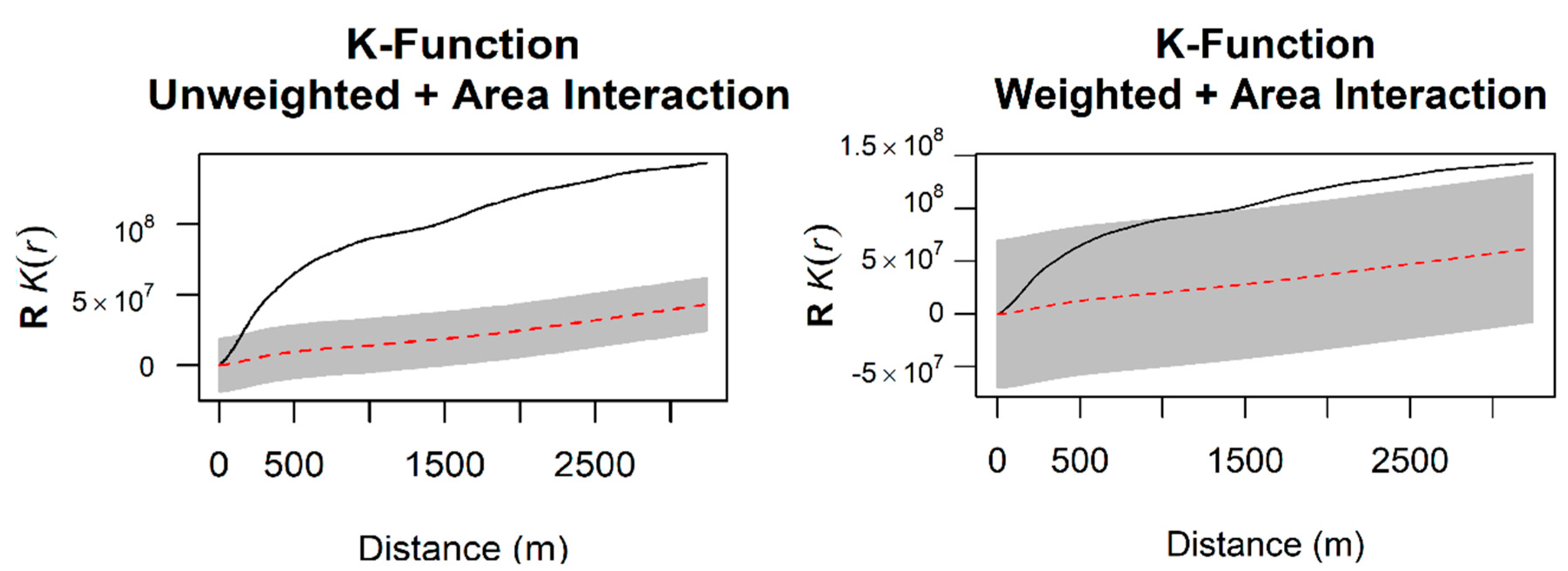
While these first-order models perform well, they underestimate the empirical distribution of archaeological deposits in some portion of the study region, suggesting the influence of some kind of second-order process on the settlement pattern. The addition of a second-order clustering process (i.e., area interaction) results in a substantial improvement to the models, decreasing model selection criteria values by thousands compared to models without second-order properties (Table 6). Combined with differential weights for environmental covariates, the settlement pattern in southwest Madagascar is best explained by environmental variables related to freshwater availability and defense, followed by marine resource access and inter-point clustering between archaeological points at some scales (Figure 9). This conclusion fits well with ethnohistoric data for coastal Vezo communities in southwest Madagascar [41,42,43,66] and provides further support of an Allee-effect distribution (as suggested by Reference [49]). Thus, we find that PPMs—and second-order properties specifically—are critical for developing and refining predictive models for landscape-scale archaeological research in this area. Nevertheless, the best fitting model is still not a perfect explanation for settlement patterns in this region, as the residual K-function shows higher rates of clustering between points at distances of ≥1500 m. This suggests that some additional factor (e.g., land governance, kinship or social networks, etc.) not accounted for by the best-fitting model is causing aggregation in archaeological materials at distances greater than 1500 m. One possibility is that foraging took place by some communities at larger distances from a primary residence, which has been demonstrated ethnographically in this region [42,43].

Our results also contribute, more specifically, to the interpretation of Madagascar’s archaeological record. Results in Table 4 suggest that archaeological settlement conforms to an ideal-free distribution (either IFD or IFD-Allee) based on the proportion of artifacts recovered from high suitability areas relative to medium and low suitability locations. This supports similar conclusions by Davis et al. [49]. The IFD predicts that as population densities increase in a given habitat, the overall resource quality in that region will decrease [51]. This degraded habitat quality, in turn, lowers the suitability of the area for future populations. Davis et al. [49] found correspondence between the archaeological settlement of the study region and an alternative model known as IFD-Allee. This model predicts that individuals sometimes benefit by settling less suitable habitats, either socially by attracting others to follow (which offsets predation and increases chances of group survival), or ecologically due to an economy of scale by modifying the surrounding area to increase its resource abundance (e.g., agriculture) [59,60,97]. In an IFD-Allee distribution, population density can decrease in higher suitability locations and increase in mid-level suitability areas [59]. Assuming that the same distribution of artifacts throughout the landscape exists as documented in Davis et al. [49] (i.e., a possible IFD-Allee), a much greater number of materials and archaeological deposits should be detected when applying the predictive model(s) developed here to new surveys in this area. This in turn will help to record at-risk cultural heritage along the coasts of Madagascar and better understand the archaeology of coastal populations in this region. While our case study focuses on coastal Madagascar, our approach can be applied to other areas as well, as long as the particular covariates included in the model are adjusted for these new contexts.

In terms of the local populations within the study region, there may be very different settlement patterns that our current models do not capture. For example, the new unweighted model (PPM6) suggests that inland dwelling groups may prioritize different resources, creating a series of “higher” suitability zones in areas currently ranked as “low” suitability. This is evidenced by the drop in artifact counts in “medium” probability areas and an increase in artifact counts in “low” probability areas (Table 4). This could also be evidence of resource control by certain populations, forcing larger communities into less suitable locations (e.g., IDD [61,62,63]). Additionally, it has been suggested that where subsistence strategies change, environmental proxies for habitat suitability will require modification [30,98]. This is because the variables associated with “suitability” (and their relative importance) change as subsistence strategies shift (e.g., fishing communities will value marine resources more than pastoralists living inland [e.g. References, [42,43,44]). As such, the differential weights of covariates within a model are likely different across time and space and between scales of interaction. Because the southwest of Madagascar contains a diverse range of foraging strategies [42,44,45,46,47,48,49,50,51,52,53,54,55,56,57,58,59,60,61,62,63,64,65,66], this pattern of artifact counts based on suitability could reflect the varied subsistence base in this region (and by extension the fluidity of how “suitability” is defined). This may help explain why the best fitting model (PPM8) still underestimates clustering at larger distances: other local contexts may differ significantly from the overall regional pattern because of fundamental differences in their social or subsistence strategies.

Therefore, defining what constitutes a “suitable” or “unsuitable” location for settlement requires additional information. One important way this can be achieved is by engaging with local histories and ethnographic research (e.g., References [76,99,100,101]). Our current project provides a good illustration of how such anthropological research methods can improve our knowledge of the past by integrating local knowledge, human behavioral ecology, and spatially explicit modeling approaches. Additionally, such strategies permit for studies of human-environment interaction that go beyond correlation, whereby formalized hypotheses are tested to evaluate associations between different variables [17,22,102,103,104].

One limitation of our study is that our model uses modern environmental data and does not currently include paleoenvironmental information. Numerous studies have demonstrated that environmental and climate conditions have fluctuated in Madagascar over the past several-thousand years [105,106,107,108]. As such, some of our variables (i.e., depth to bedrock), are likely to have been quite similar several thousand years ago while others (i.e., vegetative index values, paleodune features) were potentially quite different. Paleodunes contain many archaeological deposits today, and so they are a direct proxy for past cultural activity, but vegetative health is potentially more problematic. Future work should thus focus on better integration of paleoclimate proxies matching the temporal placement of the archaeological materials identified. In the meantime, however, our results still provide a successful method for improving detection rates of archaeological deposits, even in the absence of paleoenvironmental data.

A second limitation is that we currently lack temporal information pertaining to the archaeological materials used for our analysis. Work is ongoing to acquire chronological data for these areas but without this information we cannot extend our analysis to investigating changes in resource use over time. This will form the basis of our future work. Currently, we can specify that some of the earliest archaeological deposits in this region (that have associated radiocarbon data) date to ~2000–3000 B.P. [48]. More information is needed, however, to fully understand settlement chronologies of this region.

A final limitation is that we make no distinctions between artifact classes within the point pattern. Different artifact types (e.g., ceramics versus shell tools) may alter the best fitting PPM and provide insight into how specific activities differ across the study area. In the same vein, differences in site function (e.g., permanent settlement, seasonal foraging camp, etc.) will likely affect results of spatial analyses, as peoples’ considerations will differ based upon the nature of what they plan to do (and how long they plan to stay) in a given location. Despite these limitations, the method presented here proves useful for planning fieldwork with respect to choosing areas for archaeological survey. Furthermore, our study provides a template of how predictive modeling and landscape archaeology can be improved using an iterative process of investigating the past.

5. Conclusions

Predictive modeling has a long history in archaeology and has resulted in great improvements in archaeological settlement studies around the world [3,4,5,10,12,32,109,110,111]. Spatial statistical models can improve predictive algorithms and aid in survey projects, whereby the most probable locations for discovering archaeological deposits can be targeted. PPMs are one such spatial method that can substantially improve predictive modeling efforts for archaeological fieldwork given their ability to more fully characterize the fundamental properties of point patterns.

Our results led to the creation of several new archaeological predictive models, some of which resulted in a reduction of false positives during field assessment. Depending upon the purpose of the research, these models may be preferred. Aerial recording of Madagascar’s archaeological landscape remains limited and this results in researchers not having a firm understanding of where many archaeological materials are located [49]. For this reason, we chose the model that resulted in the greatest number of true positives. It stands to reason that a few more false detections are a good tradeoff for a large increase in true detections when the goal is to locate as many cultural materials as possible. In other research programs it very well might be more beneficial to reduce false positives at the expense of true positives and negatives, as false positives and negatives can assist in re-evaluating prior hypotheses pertaining to archaeological settlement patterns. Given the nature of our analysis, however, evaluating false negatives is difficult, as there are no definitive locations where the model predicts a total absence of archaeological materials. Nonetheless, researchers who utilize this method (or similar approaches) should investigate “low” probability locations with the same rigor as “high” probability areas to ensure that surveys are not biased based on initial model assumptions, which, as we demonstrate here, sometimes require adjustments.

Our study also demonstrates how the importance of different variables can be incorporated as weights within a predictive model using the results of spatial modeling procedures. By integrating ethnohistoric data with statistical model-selection, we improve our understanding of what constitutes a “suitable” environment (following HBE expectations from an IFD model) and increase the number of true positive identifications of archaeological materials during fieldwork. As such, we argue that archaeological survey procedures can be greatly enhanced by replicating the methods developed here. To facilitate this, all code required for performing the necessary spatial statistical tests are provided as Supplemental Files.

Ultimately, this study can serve as a template for future settlement pattern analyses using an iterative archaeological assessment. We combine robust statistical analyses, landscape scale data (via remote sensing) and traditional knowledge with explicit theoretical frameworks to account for fundamental aspects of archaeological settlement distributions. The use of PPMs allows researchers to investigate important second-order properties that are often ignored by other predictive modeling efforts. The procedure we advocate here (Figure 2) allows for a continuous learning process whereby archaeologists can evaluate different hypotheses and subsequently refine those hypotheses to improve our understanding of the past. We hope that archaeologists find this process useful for framing future landscape scale studies of past human behavior.

References

1. Bettinger, R.L. Explanatory/predictive models of hunter–gatherer adaptation. In Advances in Archaeological Method and Theory; Elsevier: Amsterdam, Netherlands, 1980; pp. 189–255. [Google Scholar]
2. Custer, J.F.; Eveleigh, T.; Klemas, V.; Wells, I. Application of Landsat Data and Synoptic Remote Sensing to Predictive Models for Prehistoric Archaeological Sites: An Example from the Delaware Coastal Plain. Am. Antiq. 1986, 51, 572–588. [Google Scholar] [CrossRef]
3. Quantifying the Present and Predicting the Past: Theory, Method, and Application of Archaeological Predictive Modeling; U.S. Department of the Interior; Judge, W.J.; Sebastian, L. (Eds.) Bureau of Land Management: Denver, CO, USA, 1988.
4. Jochim, M.A. Hunter-Gatherer Subsistence and Settlement: A Predictive Model; Academic Press: New York, NY, USA, 1976. [Google Scholar]
5. Plog, F.; Hill, J.N. Explaining variability in the distribution of sites. Distrib. Prehist. Popul. Aggreg. 1971, 1, 7. [Google Scholar]
6. Verhagen, P.; Whitley, T.G. Integrating Archaeological Theory and Predictive Modeling: A Live Report from the Scene. J. Archaeol. Method Theory 2012, 19, 49–100. [Google Scholar] [CrossRef] [Green Version]
7. Kirk, S.D.; Thompson, A.E.; Lippitt, C.D. Predictive Modeling for Site Detection Using Remotely Sensed Phenological Data. Adv. Archaeol. Pract. 2016, 4, 87–101. [Google Scholar] [CrossRef]
8. Klehm, C.; Barnes, A.; Follett, F.; Simon, K.; Kiahtipes, C.; Mothulatshipi, S. Toward archaeological predictive modeling in the Bosutswe region of Botswana: Utilizing multispectral satellite imagery to conceptualize ancient landscapes. J. Anthr. Archaeol. 2019, 54, 68–83. [Google Scholar] [CrossRef]
9. Alexakis, D.; Sarris, A.; Astaras, T.; Albanakis, K. Integrated GIS, remote sensing and geomorphologic approaches for the reconstruction of the landscape habitation of Thessaly during the neolithic period. J. Archaeol. Sci. 2011, 38, 89–100. [Google Scholar] [CrossRef]
10. Parker, S. Predictive modeling of site settlement systems using multivariate logistics. In For Concordance in Archaeological Analysis: Bridging Data Structure, Quantitative Technique and Theory; Waveland Press: New York, NY, USA, 1985; pp. 173–207. [Google Scholar]
11. Warren, R.E. Predictive modelling in archaeology: A primer. In Interpreting Space: GIS and Archaeology; Allen, K.M., Green, S.W., Zubrow, E.B.W., Eds.; Taylor and Francis: London, UK, 1990; pp. 90–111. [Google Scholar]
12. van Leusen, M.; Deeben, J.; Hallewas, D.; Zoetbrood, P.; Kamermans, H.; Verhagen, P. A baseline for predictive modelling in the Netherlands. In Predictive modelling for archaeological heritage management: A research agenda; van Leusen, M., Kamermans, H., Eds.; Rijksdienst v/h Oudheidkundig: Amsterdam, The Netherlands, 2005; pp. 25–93. [Google Scholar]
13. Howey, M.C.L.; Palace, M.W.; McMichael, C.H. Geospatial modeling approach to monument construction using Michigan from A.D. 1000–1600 as a case study. Proc. Natl. Acad. Sci. USA 2016, 113, 7443–7448. [Google Scholar] [CrossRef] [Green Version]
14. Davis, D.S.; Douglass, K. Aerial and Spaceborne Remote Sensing in African Archaeology: A Review of Current Research and Potential Future Avenues. Afr. Archaeol. Rev. 2020, 37, 9–24. [Google Scholar] [CrossRef]
15. Baddeley, A.; Rubak, E.; Turner, R. Spatial Point Patterns: Methodology and Applications with R; CRC Press: Boca Raton, FL, USA, 2015. [Google Scholar]
16. O’Sullivan, D.; Perry, G.L. Spatial Simulation: Exploring Pattern and Process; Wiley-Blackwell: Oxford, UK, 2013. [Google Scholar]
17. DiNapoli, R.J.; Lipo, C.P.; Brosnan, T.; Hunt, T.L.; Hixon, S.; Morrison, A.E.; Becker, M. Rapa Nui (Easter Island) monument (ahu) locations explained by freshwater sources. PLoS ONE 2019, 14, e0210409. [Google Scholar] [CrossRef]
18. Bevan, A.; Crema, E.; Palmisano, A. Intensities, interactions and uncertainties: Some new approaches to archaeological distributions. In Computational Approaches to Archaeological Spaces; Bevan, A., Lake, M., Eds.; Left Coast Press: Walnut Creek, CA, USA, 2013; pp. 27–52. [Google Scholar]
19. Carrero-Pazos, M.; Bevan, A.; Lake, M.W. The spatial structure of Galician megalithic landscapes (NW iberia): A case study from the Monte Penide region. J. Archaeol. Sci. 2019, 108, 104968. [Google Scholar] [CrossRef]
20. Davis, D.S.; DiNapoli, R.J.; Sanger, M.C.; Lipo, C.P. The integration of lidar and legacy datasets provides improved explanations for the spatial patterning of shell rings in the American Southeast. Adv. Archaeol. Pract. 2020, in press. [Google Scholar] [CrossRef]
21. Brandolini, F.; Carrer, F. Terra, Silva et Paludes Assessing the Role of Alluvial Geomorphology for Late-Holocene Settlement Strategies (Po Plain – N Italy) Through Point Pattern Analysis. Environ. Archaeol. 2020, 1–15. [Google Scholar] [CrossRef]
22. Eve, S.J.; Crema, E.R. A house with a view? Multi-model inference, visibility fields and point process analysis of a Bronze Age settlement on Leskernick Hill (Cornwall, UK). J. Archaeol. Sci. 2014, 43, 267–277. [Google Scholar] [CrossRef] [Green Version]
23. Bevan, A.; Conolly, J. Terraced fields and Mediterranean landscape structure: An analytical case study from Antikythera, Greece. Ecol. Model. 2011, 222, 1303–1314. [Google Scholar] [CrossRef]
24. Bevan, A.; Jobbová, E.; Helmke, C.; Awe, J.J. Directional layouts in central lowland Maya settlement. J. Archaeol. Sci. 2013, 40, 2373–2383. [Google Scholar] [CrossRef] [Green Version]
25. Bevan, A.; Lake, M. Intensities, interactions and uncertainties: Some new approaches to archaeological distributions. In Computational Approaches to Archaeological Spaces; Routledge: Abingdon, UK, 2016; pp. 27–52. [Google Scholar]
26. Bevan, A.; Wilson, A. Models of settlement hierarchy based on partial evidence. J. Archaeol. Sci. 2013, 40, 2415–2427. [Google Scholar] [CrossRef]
27. Carrero-Pazos, M. Density, intensity and clustering patterns in the spatial distribution of Galician megaliths (NW Iberian Peninsula). Archaeol. Anthr. Sci. 2019, 11, 2097–2108. [Google Scholar] [CrossRef]
28. Carrero-Pazos, M.; Bustelo-Abuín, J.; Barbeito-Pose, V.; Rodríguez-Rellán, C. Locational preferences and spatial arrangement in the barrow landscape of Serra do Barbanza (North-western Iberia). J. Archaeol. Sci. Rep. 2020, 31, 102351. [Google Scholar] [CrossRef]
29. Spencer, C.; Bevan, A. Settlement location models, archaeological survey data and social change in Bronze Age Crete. J. Anthr. Archaeol. 2018, 52, 71–86. [Google Scholar] [CrossRef]
30. Vernon, K.B.; Yaworsky, P.M.; Spangler, J.; Brewer, S.; Codding, B.F. Decomposing Habitat Suitability Across the Forager to Farmer Transition. Environ. Archaeol. 2020, 1–14, in press. [Google Scholar] [CrossRef]
31. Knitter, D.; Nakoinz, O. Point Pattern Analysis as Tool for Digital Geoarchaeology: A Case Study of Megalithic Graves in Schleswig-Holstein, Germany. In Digital Geoarchaeology: New Techniques for Interdisciplinary Human-Environmental Research; Siart, C., Forbriger, M., Bubenzer, O., Eds.; Natural Science in Archaeology; Springer International Publishing: Cham, Switzerland, 2018; pp. 45–64. ISBN 978-3-319-25316-9. [Google Scholar]
32. Hamer, W.B.; Knitter, D.; Grimm, S.B.; Serbe, B.; Eriksen, B.V.; Nakoinz, O.; Duttmann, R. Location Modeling of Final Palaeolithic Sites in Northern Germany. Geosciences 2019, 9, 430. [Google Scholar] [CrossRef] [Green Version]
33. Beaujard, P. East Africa, the Comoros Islands and Madagascar before the sixteenth century: On a neglected part of the world system. Azania Archaeol. Res. Afr. 2007, 42, 15–35. [Google Scholar] [CrossRef]
34. Beaujard, P. The first migrants to Madagascar and their introduction of plants: Linguistic and ethnological evidence. Azania Archaeol. Res. Afr. 2011, 46, 169–189. [Google Scholar] [CrossRef] [Green Version]
35. Boivin, N.; Crowther, A.; Helm, R.; Fuller, D.Q. East Africa and Madagascar in the Indian Ocean world. J. World Prehistory 2013, 26, 213–281. [Google Scholar] [CrossRef]
36. Radimilahy, C.M.; Crossland, Z. Situating Madagascar: Indian Ocean dynamics and archaeological histories. Azania Archaeol. Res. Afr. 2015, 50, 495–518. [Google Scholar] [CrossRef]
37. Mitchell, P. Settling Madagascar: When Did People First Colonize the World’s Largest Island? J. Isl. Coast. Archaeol. 2019, 1–20. [Google Scholar] [CrossRef]
38. Hansford, J.; Wright, P.C.; Rasoamiaramanana, A.; Pérez, V.R.; Godfrey, L.R.; Errickson, D.; Thompson, T.; Turvey, S.T. Early Holocene human presence in Madagascar evidenced by exploitation of avian megafauna. Sci. Adv. 2018, 4, eaat6925. [Google Scholar] [CrossRef] [Green Version]
39. Anderson, A.; Clark, G.; Haberle, S.; Higham, T.; Nowak-Kemp, M.; Prendergast, A.; Radimilahy, C.; Rakotozafy, L.M.; Virah-Sawmy, M.; Schwenninger, J.-L.; et al. New evidence of megafaunal bone damage indicates late colonization of Madagascar. PLoS ONE 2018, 13, e0204368. [Google Scholar] [CrossRef]
40. Douglass, K.; Hixon, S.; Wright, H.T.; Godfrey, L.R.; Crowley, B.E.; Manjakahery, B.; Rasolondrainy, T.; Crossland, Z.; Radimilahy, C. A critical review of radiocarbon dates clarifies the human settlement of Madagascar. Quat. Sci. Rev. 2019, 221, 105878. [Google Scholar] [CrossRef]
41. Astuti, R. The People of the Sea: Identity and Decent among the Vezo of Madagascar; Cambridge University Press: Cambridge, UK, 1995. [Google Scholar]
42. Iida, T. The past and present of the coral reef fishing economy in Madagascar: Implications for self-determination in resource use. Senri Ethnol. Stud. 2005, 67, 237–258. [Google Scholar]
43. Koechlin, B. Es Vezo du Sud-Ouest de Madagascar: Contribution à l’étude de l’éco-système de Semi-Nomades Marins; Mouton & Co: Paris, France, 1975. [Google Scholar]
44. Yount, J.W.; Tucker, B.T. Constructing Mikea Identity: Past or Present Links to Forest and Foraging. Ethnohistory 2001, 48, 257–291. [Google Scholar] [CrossRef]
45. Tucker, B.; Tsimitamby, M.; Humber, F.; Benbow, S.; Iida, T. Foraging for Development: A Comparison of Food Insecurity, Production and Risk among Farmers, Forest Foragers and Marine Foragers in Southwestern Madagascar. Hum. Organ. 2010, 69, 375–386. [Google Scholar] [CrossRef]
46. Dewar, R.E.; Radimilahy, C.; Wright, H.T.; Jacobs, Z.; Kelly, G.O.; Berna, F. Stone tools and foraging in northern Madagascar challenge Holocene extinction models. Proc. Natl. Acad. Sci. USA 2013, 110, 12583–12588. [Google Scholar] [CrossRef] [PubMed] [Green Version]
47. Parker Pearson, M.; Godden, K.; Ramilisonina, R.; Schwenninger, J.; Heurtebize, G.; Radimilahy, C.; Smith, H. Pastoralists, Warriors and Colonists: The Archaeology of Southern Madagascar; BAR International Series; Archaeopress: Oxford, UK, 2010. [Google Scholar]
48. Douglass, K. An Archaeological Investigation of Settlement and Resource Exploitation Patterns in the Velondriake Marine Protected Area, Southwest Madagascar, Ca. 900 BC to AD 1900. Ph.D. Thesis, Yale University, New Haven, CT, USA, 2016. [Google Scholar]
49. Davis, D.S.; Andriankaja, V.; Carnat, T.L.; Chrisostome, Z.M.; Colombe, C.; Fenomanana, F.; Hubertine, L.; Justome, R.; Lahiniriko, F.; Léonce, H.; et al. Satellite-based remote sensing rapidly reveals extensive record of Holocene coastal settlement on Madagascar. J. Archaeol. Sci. 2020, 115, 105097. [Google Scholar] [CrossRef]
50. Charnov, E.L. Optimal Foraging, the Marginal Value Theorem. Theor. Popul. Biol. 1976, 9, 129–136. [Google Scholar] [CrossRef] [Green Version]
51. Fretwell, S.D.; Lucas, H.L. On territorial behavior and other factors influencing habitat distribution in birds: I. Theoretical development. Acta Biotheor. 1969, 19, 16–36. [Google Scholar] [CrossRef]
52. MacArthur, R.H.; Pianka, E.R. On Optimal Use of a Patchy Environment. Am. Nat. 1966, 100, 603–609. [Google Scholar] [CrossRef] [Green Version]
53. Douglass, K.; Quintana Morales, E.M.; Rasolondrainy, T.; Manahira, G.; Manjakahery, B.; Rosily; Ediedy, A.; Mampibay, F.; Rabekoto, H.; Rasoafiavy, P.; et al. The Vezo Ecological Knowledge Exchange. J. Ethnobiol. in preparation.
54. Lane, P.J. Archaeology in the age of the Anthropocene: A critical assessment of its scope and societal contributions. J. Field Archaeol. 2015, 40, 485–498. [Google Scholar] [CrossRef]
55. Huntington, H.; Callaghan, T.; Fox, S.; Krupnik, I. Matching Traditional and Scientific Observations to Detect Environmental Change: A Discussion on Arctic Terrestrial Ecosystems. AMBIO 2004, 33, 18–23. [Google Scholar] [CrossRef]
56. Cooper, J.; Sheets, P. Surviving Sudden Environmental Change: Answers from Archaeology; University Press of Colorado: Boulder, CT, USA, 2012. [Google Scholar]
57. Lefale, P.F. Ua ‘afa le Aso Stormy weather today: Traditional ecological knowledge of weather and climate. The Samoa experience. Clim. Chang. 2010, 100, 317–335. [Google Scholar] [CrossRef] [Green Version]
58. Cooper, J.; Duncan, L. Applied Archaeology in the Americas: Evaluating Archaeological Solutions to the Impacts of Global Environmental Change. In The Oxford Handbook of Historical Ecology and Applied Archaeology; Isendahl, C., Stump, D., Eds.; Oxford University Press: Oxford, UK, 2019; pp. 440–458. ISBN 978-0-19-967269-1. [Google Scholar]
59. Winterhalder, B.; Kennett, D.J.; Grote, M.N.; Bartruff, J. Ideal free settlement of California’s Northern Channel Islands. J. Anthr. Archaeol. 2010, 29, 469–490. [Google Scholar] [CrossRef] [Green Version]
60. Bliege Bird, R.; McGuire, C.; Bird, D.W.; Price, M.H.; Zeanah, D.; Nimmo, D.G. Fire mosaics and habitat choice in nomadic foragers. Proc. Natl. Acad. Sci. USA 2020, 117, 201921709. [Google Scholar] [CrossRef] [PubMed]
61. Jazwa, C.S.; Kennett, D.J.; Winterhalder, B.; Joslin, T.L. Territoriality and the rise of despotic social organization on western Santa Rosa Island, California. Quat. Int. 2017, 518, 41–56. [Google Scholar] [CrossRef] [Green Version]
62. Summers, K. The evolutionary ecology of despotism. Evol. Hum. Behav. 2005, 26, 106–135. [Google Scholar] [CrossRef]
63. Bell, A.V.; Winterhalder, B. The Population Ecology of Despotism. Hum. Nat. 2014, 25, 121–135. [Google Scholar] [CrossRef] [Green Version]
64. Huete, A.R. A soil-adjusted vegetation index (SAVI). Remote Sens. Environ. 1988, 25, 295–309. [Google Scholar] [CrossRef]
65. Tucker, B. Où vivre sans boire revisited: Water and political-economic change among Mikea hunter-gatherers of southwestern Madagascar. Econ. Anthr. 2020, 7, 22–37. [Google Scholar] [CrossRef]
66. Langley, J.M. Vezo Knowledge: Traditional Ecological Knowledge in Andavadoaka, southwest Madagascar; Blue Ventures: London, UK, 2006; p. 73. [Google Scholar]
67. Douglass, K.; Walz, J.; Quintana-Morales, E.; Marcus, R.; Myers, G.; Pollini, J. Historical perspectives on contemporary human-environment dynamics in southeast Africa. Conserv. Biol. 2019, 33, 260–274. [Google Scholar] [CrossRef]
68. Fishman, R.M.; Siegfried, T.; Raj, P.; Modi, V.; Lall, U. Over-extraction from shallow bedrock versus deep alluvial aquifers: Reliability versus sustainability considerations for India’s groundwater irrigation. Water Resour. Res. 2011, 47, 6. [Google Scholar] [CrossRef] [Green Version]
69. Gabrielli, C.P.; McDonnell, J.J.; Jarvis, W.T. The role of bedrock groundwater in rainfall–runoff response at hillslope and catchment scales. J. Hydrol. 2012, 450, 117–133. [Google Scholar] [CrossRef]
70. Hengl, T.; Heuvelink, G.B.; Kempen, B.; Leenaars, J.G.; Walsh, M.G.; Shepherd, K.D.; Sila, A.; MacMillan, R.A.; de Jesus, J.M.; Tamene, L. Mapping soil properties of Africa at 250 m resolution: Random forests significantly improve current predictions. PLoS ONE 2015, 10, e0125814. [Google Scholar] [CrossRef] [PubMed]
71. Appels, W.M.; Graham, C.B.; Freer, J.E.; McDonnell, J.J. Factors affecting the spatial pattern of bedrock groundwater recharge at the hillslope scale. Hydrol. Process. 2015, 29, 4594–4610. [Google Scholar] [CrossRef] [Green Version]
72. Hopp, L.; McDonnell, J.J. Connectivity at the hillslope scale: Identifying interactions between storm size, bedrock permeability, slope angle and soil depth. J. Hydrol. 2009, 376, 378–391. [Google Scholar] [CrossRef]
73. Brosnan, T.; Becker, M.W.; Lipo, C.P. Coastal groundwater discharge and the ancient inhabitants of Rapa Nui (Easter Island), Chile. Hydrogeol. J. 2018, 27, 519–534. [Google Scholar] [CrossRef]
74. Brenan, P. The Geology of Madagascar. In Biogeography and Ecology in Madagascar; Battistini, R., Richard-Vindard, G., Eds.; Springer Netherlands: Dordrecht, The Netherlands, 1972; Volume 21, pp. 27–86. ISBN 978-94-015-7161-6. [Google Scholar]
75. Douglass, K. The Diversity of Late Holocene Shellfish Exploitation in Velondriake, Southwest Madagascar. J. Isl. Coast. Archaeol. 2017, 12, 333–359. [Google Scholar] [CrossRef]
76. Douglass, K.; Morales, E.Q.; Manahira, G.; Fenomanana, F.; Samba, R.; Lahiniriko, F.; Chrisostome, Z.M.; Vavisoa, V.; Soafiavy, P.; Justome, R.; et al. Toward a just and inclusive environmental archaeology of southwest Madagascar. J. Soc. Archaeol. 2019, 19, 307–332. [Google Scholar] [CrossRef]
77. Ripley, B.D. Modelling spatial patterns. J. R. Stat. Soc. Ser. B Methodol. 1977, 39, 172–192. [Google Scholar] [CrossRef]
78. Stoyan, D.; Stoyan, H. Fractals, Random Shapes and Point Fields: Methods of Geometrical Statistics; John Wiley & Sons Inc.: Hoboken, NJ, USA, 1994; Volume 302. [Google Scholar]
79. Akaike, H. A New Look at the Statistical Model Identification. In Selected Papers of Hirotugu Akaike; Parzen, E., Tanabe, K., Kitagawa, G., Eds.; Springer: New York, NY, USA, 1974; pp. 215–222. ISBN 978-1-4612-7248-9. [Google Scholar]
80. Burnham, K.P.; Anderson, D.R. Model Selection and Multimodel inference: A Practical Information-Theoretic Approach, 2nd ed.; Springer: New York, NY, USA, 2002. [Google Scholar]
81. Schwarz, G. Estimating the Dimension of a Model. Ann. Stat. 1978, 6, 461–464. [Google Scholar] [CrossRef]
82. Venables, W.N.; Ripley, B.D. Modern Applied Statistics with S, 4th ed.; Springer: New York, NY, USA, 2002; ISBN 0-387-95457-0. [Google Scholar]
83. Baddeley, A.; Turner, R.; Møller, J.; Hazelton, M. Residual analysis for spatial point processes (with discussion). J. R. Stat. Soc. Ser. B Stat. Methodol. 2005, 67, 617–666. [Google Scholar] [CrossRef] [Green Version]
84. Baddeley, A.; Rubak, E.; Møller, J. Score, pseudo-score and residual diagnostics for spatial point process models. Stat. Sci. 2011, 26, 613–646. [Google Scholar] [CrossRef] [Green Version]
85. ESRI ArcGIS. Environmental Systems Research Institute; ESRI ArcGIS: Redlands, CA, USA, 2019. [Google Scholar]
86. QGIS Development Team. QGIS Geographic Information System; Open Source Geospatial Foundation Project; 2018. Available online: https://qgis.org/en/site/ (accessed on 27 July 2020).
87. Jenks, G.F. The data model concept in statistical mapping. Int. Yearb. Cartogr. 1967, 7, 186–190. [Google Scholar]
88. R Core Team R. A Language and Environment for Statistical Computing; R Foundation for Statistical Computing: Vienna, Austria, 2019. [Google Scholar]
89. Barton, K. MuMIn: Multi-Model Inference; 2019. Available online: https://r-forge.r-project.org/R/?group_id=346 (accessed on 27 July 2020).
90. Bivand, R.; Lewin-Koh, N. Maptools: Tools for Handling Spatial Objects; 2019. Available online: https://cran.r-project.org/web/packages/maptools/index.html (accessed on 27 July 2020).
91. Hijmans, R.J. Raster: Geographic Data Analysis and Modeling; 2019. Available online: https://cran.r-project.org/web/packages/raster/index.html (accessed on 27 July 2020).
92. Bivand, R.; Keitt, T.; Rowlingson, B. Rgdal: Bindings for the “Geospatial” Data Abstraction Library; 2019. Available online: https://cran.r-project.org/web/packages/rgdal/index.html (accessed on 27 July 2020).
93. Bivand, R.; Rundel, C. Rgeos: Interface to Geometry Engine—Open Source (‘GEOS’); 2019. Available online: https://cran.r-project.org/web/packages/rgeos/index.html (accessed on 27 July 2020).
94. Bivand, R.S.; Pebesma, E.J.; Gomez-Rubio, V.; Pebesma, E.J. Applied Spatial Data Analysis with R, 2nd ed.; Springer: New York, NY, USA, 2013. [Google Scholar]
95. Pebesma, E.J.; Bivand, R.S. Classes and methods for spatial data in R. R News 2005, 5, 9–13. [Google Scholar]
96. Baddeley, A.J.; van Lieshout, M.N.M. Area-interaction point processes. Ann. Inst. Stat. Math. 1995, 47, 601–619. [Google Scholar] [CrossRef] [Green Version]
97. Angulo, E.; Luque, G.M.; Gregory, S.D.; Wenzel, J.W.; Bessa-Gomes, C.; Berec, L.; Courchamp, F. Review: Allee effects in social species. J. Anim. Ecol. 2018, 87, 47–58. [Google Scholar] [CrossRef] [PubMed] [Green Version]
98. Plekhov, D.; Levine, E.I. Defining Suitability in Mixed Agropastoral Societies: A Case Study from Bactria in Northern Afghanistan. Environ. Archaeol. 2020, 1–16. [Google Scholar] [CrossRef]
99. Green, L.F.; Green, D.R.; Neves, E.G. Indigenous Knowledge and Archaeological Science: The Challenges of Public Archaeology in the Reserva Uaçá. J. Soc. Archaeol. 2003, 3, 366–398. [Google Scholar] [CrossRef]
100. Moser, S.; Glazier, D.; Phillips, J.E.; el Nemr, L.N.; Mousa, M.S.; Aiesh, R.N.; Richardson, S.; Conner, A.; Seymour, M. Transforming archaeology through practice: Strategies for collaborative archaeology and the Community Archaeology Project at Quseir, Egypt. World Archaeol. 2002, 34, 220–248. [Google Scholar] [CrossRef]
101. Gallivan, M.; Moretti-Langholtz, D.; Woodard, B. Collaborative archaeology and strategic essentialism: Native empowerment in Tidewater Virginia. Hist. Archaeol. 2011, 45, 10–23. [Google Scholar] [CrossRef]
102. Davis, D.S. Studying human responses to environmental change: Trends and trajectories of archaeological research. Environ. Archaeol. 2019, 1–15, in press. [Google Scholar] [CrossRef]
103. d’Alpoim Guedes, J.A.; Crabtree, S.A.; Bocinsky, R.K.; Kohler, T.A. Twenty-first century approaches to ancient problems: Climate and society. Proc. Natl. Acad. Sci. USA 2016, 113, 14483–14491. [Google Scholar] [CrossRef] [PubMed] [Green Version]
104. Contreras, D.A. Correlation is not enough: Building better arguments in the archaeology of human-environment interactions. In The Archaeology of Human-Environment Interactions; Routledge: Abingdon, UK, 2016; pp. 17–36. [Google Scholar]
105. Virah-Sawmy, M.; Willis, K.J.; Gillson, L. Evidence for drought and forest declines during the recent megafaunal extinctions in Madagascar. J. Biogeogr. 2010, 37, 506–519. [Google Scholar] [CrossRef]
106. Burney, D.A. Rates, Patterns and Processes of Landscape Transformation and Extinction in Madagascar. In Extinctions in Near Time; MacPhee, R.D.E., Ed.; Springer US: Boston, MA, USA, 1999; pp. 145–164. ISBN 978-1-4419-3315-7. [Google Scholar]
107. Hixon, S.W.; Elliott Smith, E.A.; Crowley, B.E.; Perry, G.H.; Randrianasy, J.; Ranaivoarisoa, J.F.; Kennett, D.J.; Newsome, S.D. Nitrogen isotope (δ 15 N) patterns for amino acids in lemur bones are inconsistent with aridity driving megafaunal extinction in south-western Madagascar: Megafaunal Extinction in South-Western Madagascar. J. Quat. Sci. 2018, 33, 958–968. [Google Scholar] [CrossRef]
108. Godfrey, L.R.; Scroxton, N.; Crowley, B.E.; Burns, S.J.; Sutherland, M.R.; Pérez, V.R.; Faina, P.; McGee, D.; Ranivoharimanana, L. A new interpretation of Madagascar’s megafaunal decline: The “Subsistence Shift Hypothesis”. J. Hum. Evol. 2019, 130, 126–140. [Google Scholar] [CrossRef] [PubMed]
109. Kvamme, K.L. A Manual for Predictive Site Location Models: Examples from the Grand Junction District, Colorado; Bureau of Land Management: Grand Junction District, CO, USA, 1983.
110. Altschul, J.H. Models and the Modeling Process. In Quantifying the Present and Predicting the Past: Theory, Method, and Application of Archaeological Predictive Modeling; Judge, W.J., Sebastian, L., Eds.; US Department of the Interior, Bureau of Land Management: Denver, CO, USA, 1988; pp. 61–96. [Google Scholar]
111. Green, E.L. Location analysis of prehistoric Maya sites in Northern British Honduras. Am. Antiq. 1973, 38, 279–293. [Google Scholar] [CrossRef]
Figure 1. Map of study region in southwest Madagascar. The region contains the Velondriake Marine Protected Area and has been increasingly documented by archaeologists over the past several years.
Geosciences 10 00287 g001
Figure 2. Illustration of iterative modeling process. This method permits for simultaneous and constant re-evaluation of the current predictive model and interpretation of the archaeological record.
Geosciences 10 00287 g002
Figure 3. Left: shows the unweighted predictive raster without resampling depth to bedrock data from 150 m to 10 m. Right: shows the results of the unweighted predictive raster after resampling depth to bedrock data from 150 m to 10 m. Resampling makes the results more easily interpretable and by extension, usable for archaeological survey.
Geosciences 10 00287 g003
Figure 4. First order intensity of archaeological deposits (per m2) as a function of different environmental variables using nonparametric smoothing (rho-hat test). Euclidian distance measurements were used for distance (m) calculations.
Geosciences 10 00287 g004
Figure 5. First order intensity of archaeological deposits (per m2) weighted by artifact counts as a function of different environmental variables using nonparametric smoothing (rho-hat test). Likewise to the unweighted rho-hat tests, bedrock, islands and rock outcrops have the highest absolute intensity values, while dunes and vegetation have the lowest.
Geosciences 10 00287 g005
Figure 6. Results of testing for second-order interaction using K-, G- and PC-functions compared to 39 simulated realizations of complete spatial randomness (CSR). Black line is the empirical function for archaeological deposits, the red-dashed lines is the theoretical expectation under the null model of CSR, the grey shaded region is the simulation envelope (equivalent to p = 0.05).
Geosciences 10 00287 g006
Figure 7. Map of raw and kernel-smoothed Pearson residual values of PPM3, PPM4 and PPM1. Note that the smoothed Pearson residuals for PPM3 and PPM4 contain more values of 0 (indicating a better fit), while PPM1 has more values greater than and less than 0, indicating more over- and under-fitting. Archaeological points are overlaid on top of the raw residual maps (black dots).
Geosciences 10 00287 g007
Figure 8. Results of the residual K- and G-function tests on PPM1 (the Davis et al. [49] model) and best fitted models PPM3 and PPM4. Both PPM3 and PPM4 perform better than the Davis et al. algorithm but still overestimate clustering between points at some distances.
Geosciences 10 00287 g008
Figure 9. Residual K-function test of the best-fitting unweighted PPM with an area interaction parameter and the best-fitting weighted PPM with an area interaction parameter. Both models performed better with area interaction than without and the weighted model yields the best results.
Geosciences 10 00287 g009