Soil Liquefaction Assessment Using Soft Computing Approaches Based on Capacity Energy Concept
by

Zhixiong Chen
1,2,3, 
Hongrui Li
2,
Anthony Teck Chee Goh
4,
Chongzhi Wu
2 and
Wengang Zhang
1,2,3,* 1
Key Laboratory of New Technology for Construction of Cities in Mountain Area, Chongqing University, Ministry of Education, Chongqing 400045, China
2
School of Civil Engineering, Chongqing University, Chongqing 400045, China
3
National Joint Engineering Research Center of Geohazards Prevention in the Reservoir Areas, Chongqing University, Chongqing 400045, China
4
School of Civil and Environmental Engineering, Nanyang Technological University, Singapore 639798, Singapore
*
Author to whom correspondence should be addressed.
Geosciences 2020, 10(9), 330; https://0-doi-org.brum.beds.ac.uk/10.3390/geosciences10090330
Submission received: 18 July 2020
/
Revised: 14 August 2020
/
Accepted: 19 August 2020
/
Published: 21 August 2020
(This article belongs to the Special Issue Applications of Artificial Intelligence and Machine Learning in Geotechnical Engineering)
Abstract
:Soil liquefaction is one of the most complicated phenomena to assess in geotechnical earthquake engineering. The conventional procedures developed to determine the liquefaction potential of sandy soil deposits can be categorized into three main groups: Stress-based, strain-based, and energy-based procedures. The main advantage of the energy-based approach over the remaining two methods is the fact that it considers the effects of strain and stress concurrently unlike the stress or strain-based methods. Several liquefaction evaluation procedures and approaches have been developed relating the capacity energy to the initial soil parameters, such as the relative density, initial effective confining pressure, fine contents, and soil textural properties. In this study, based on the capacity energy database by Baziar et al. (2011), analyses have been carried out on a total of 405 previously published tests using soft computing approaches, including Ridge, Lasso & LassoCV, Random Forest, eXtreme Gradient Boost (XGBoost), and Multivariate Adaptive Regression Splines (MARS) approaches, to assess the capacity energy required to trigger liquefaction in sand and silty sands. The results clearly prove the capability of the proposed models and the capacity energy concept to assess liquefaction resistance of soils. It is also proposed that these approaches should be used as cross-validation against each other. The result shows that the capacity energy is most sensitive to the relative density.
1. Introduction
Liquefaction is a catastrophic ground failure, which usually occurs in loose saturated soil deposits under earthquake excitations. After the disastrous damage observed during the Niigata and Alaska 1964 earthquakes, the liquefaction phenomenon became the scope of many studies in the field of geotechnical earthquake engineering [1,2,3]. A few systems have been created to assess the liquefaction potential in the field [4]. The accessible assessment systems can be arranged into three main gatherings: (1) Stress-based techniques, (2) strain-based methodology, and (3) energy-based strategies.
The stress-based methodology is the most broadly received strategy for liquefaction evaluation [2,5]. This strategy is predominantly empirical and depends on lab and field studies. The cyclic shear stress ratio and the cyclic resistance ratio are the significant criteria in this strategy. To correlate the real seismic motion to the laboratory harmonic loading conditions, the equivalent stress intensity and the loading cycles must be characterized [2]. Seed et al. [3] suggested the equivalent stress as 65% of the maximum shear stress, while Ishihara and Yasuda [6] proposed 57% for 20 cycles of loading.
Some probabilistic frameworks for assessing liquefaction potential of soils based on in situ tests, such as the cone penetration test (CPT) or standard penetration test (SPT), were also carried out [7,8,9,10,11]. Despite the fact that the stress-based procedure has been continuously revised and extended in subsequent studies and the database of liquefaction case histories expanded, the uncertainty concerning random loading still persists [12,13].
Several probabilistic studies have been published that have examined the liquefaction potential of soils dependent on in situ tests, for example, the CPT or SPT [7,8,9,10]. Even though the stress-based approach has been continuously updated and the liquefaction case histories expanded, there are still a number of obstacles to this process, for instance, the uncertainty of random loading [12,13].
Dobry et al. [14] suggested a strain-based approach which originated from the model of two sand grain system and then extend to the actual soil layers. In this model, pore water pressure started to evolve only when the shear strain surpassed a threshold shear strain (around 0.01%), irrespective of sand type, relative density, initial effective confining pressure, and sample preparation method. This strain-based approach is less popular than the stress-based procedure because it is much more difficult to estimate the cyclic strain compared with the cyclic shear stress [15].
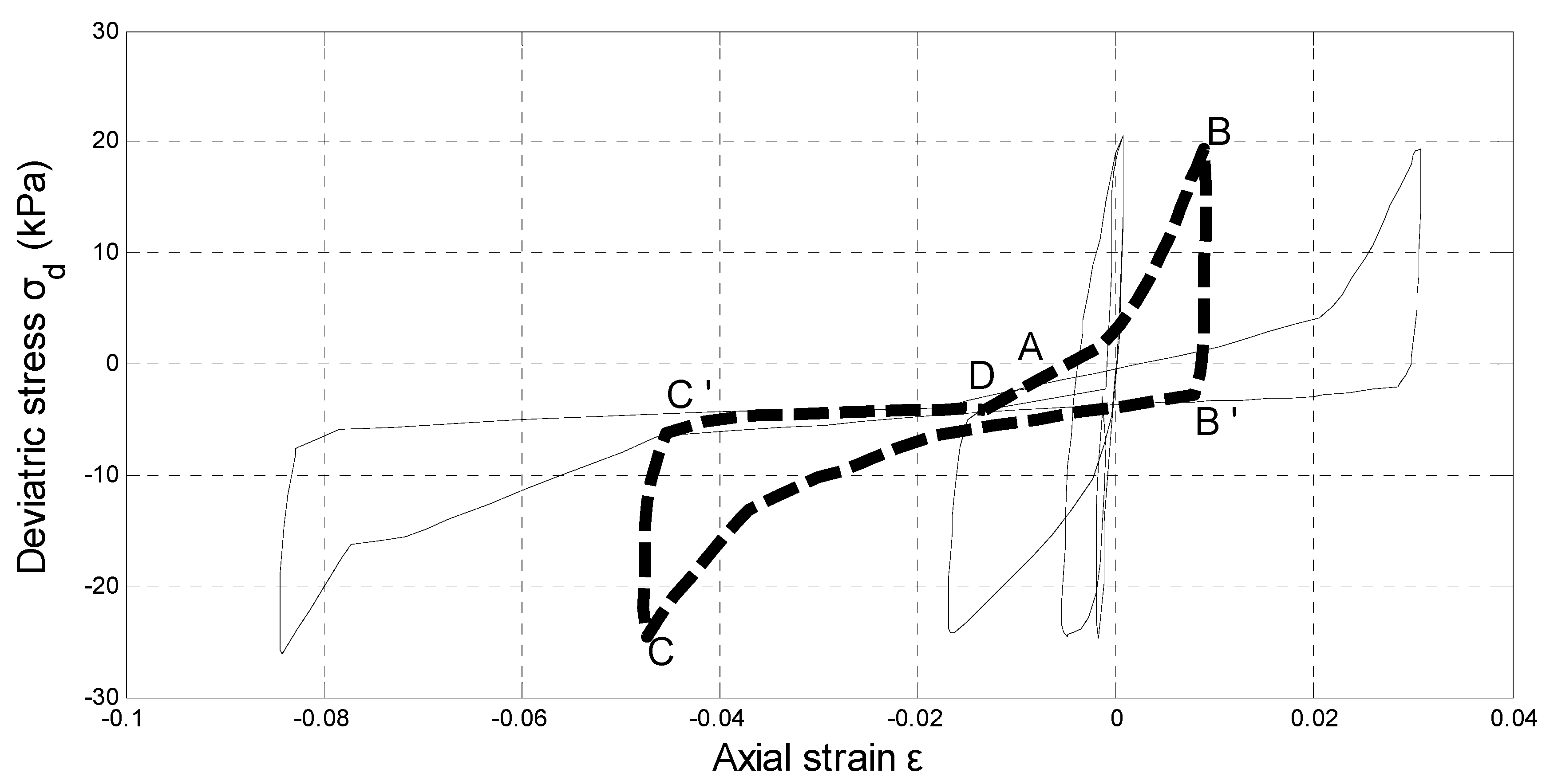
Davis and Berrill [16] introduced an energy-based approach for liquefaction potential assessment following the assumption by Nemat-Nasser and Shokooh [17] that the pore-pressure buildup had direct relations with the seismic energy dissipated in the unit volume of soil. The energy-based method absorbs the basic of both the stress and strain approach. Total strain energy at the onset of liquefaction can be calculated from laboratory or field tests. Figure 1 shows typical stress–strain relationship of undrained cyclic triaxial test. The hysteretic area enveloped by a thick dashed curve A-B-C-D represents the dissipated energy per unit volume for a kth stress cycle. The total dissipated energy summed up from the start to the onset of liquefaction cycle is [18]:
The summation of the energy describes the capacity of the soil sample against initial liquefaction.
The energy-based approach has some main advantages in evaluating the liquefaction possibility of soils [13,19]:
(1) Energy associates with both shear stress and shear strain;
(2) The dissipated energy correlates very well with the pore pressure buildup, no matter how complicated the stress–strain history is, how many cycles, or how large the applied stress ratio.
(3) Energy has strong correlation with the character of earthquake, for example, the duration and the number of cycles of the seismic wave. Furthermore, it considers the entire spectrum of ground motions, while the stress-based approach uses only the peak value of ground acceleration.
The energy-based liquefaction evaluation methods fall into two main categories: One using earthquake case histories, and the other based on laboratory cyclic shear and centrifuge tests [12]. Many researchers have developed the soil liquefaction prediction model considering the effective mean confining pressure and initial relative density [20,21,22], mainly by performing multiple linear regression (MLR) analysis. These models can obtain high correlation coefficient R values, but generally they are based on a limited number of tests and fail to consider the important role of the fines content.
Besides, Baziar and Jafarian [13] showed that these formulas could not work well in a large data set of various types of sand. Using their updated database, Baziar and Jafarian [13] demonstrated the unacceptable performance of MLR-based relationship and highlighted the need of developing an artificial neural network (ANN)-based model. Moreover, Chen et al. [23] proposed a seismic wave energy-based method with back-propagation neural networks to evaluate the liquefaction probability. Despite the good performance of the ANN-based models, the black-box nature restricts their practical applications.
Baziar et al. [19] suggested a genetic programming (GP) evolutionary approach to predict the capacity energy of liquefiable soils after expanding the database. Alavi and Gandomi [24] improved the GP and provided linear genetic programming (LGP) and multi-expression programming (MEP) to evaluate the liquefaction resistance of sandy soils. Cabalar et al. [25] presented an Adaptive Neuro-Fuzzy Inference System (ANFIS) for the prediction of liquefaction triggering, which possesses the natural language description of fuzzy systems and the learning capability of neural networks.
The multivariate adaptive regression splines (MARS) model can give the explicit expression, is much easier to interpret, and can provide the relative importance of the input variables [26,27,28,29,30,31,32,33,34,35,36,37,38,39,40,41]. In this study, based on the capacity energy database by Baziar et al. [19], analyses have been carried out on a total of 405 previously published tests using soft computing techniques, including Ridge, Lasso & Lasso CV, Random Forest, eXtreme Gradient Boost (XGBoost) and MARS approaches, to assess the capacity energy required to trigger liquefaction in sand and silty sands. The capacity energies estimated by these proposed models compare favorably with the testing data sets used for validation purpose. It is also proposed that these approaches should be used as cross-validation against each other.
2. Machine Learning Methodology
2.1. Ridge Regression Algorithm
The method of Ridge regression, proposed by Hoerl and Kennard [42], has been used extensively for dealing with the problem of multicollinearity in regression. Multicollinearity is the existence of near-linear relationships among the independent variables. The multicollinearity may cause a great error in the ordinary least squares (OLS) method by giving large regression coefficients with unstable signs [43]. The ridge regression method introduces an additional ridge parameter to control this regression bias. For example, a widely used linear regression model has the form of:
In which Y is a vector of observations on a response variable. is a vector of regression coefficients to be estimated, X is a matrix of order () of observations on ‘p’ regressor variables. represents an vector of residuals (errors).
In ordinary least squares, the regression coefficient is estimated using the formula:
Whenever the multicollinearity presents in the data, the OLS estimator may create inaccurate estimates of the regression coefficients. The matrix of XTX is singular. The eigenvalues of the matrix are small, which results in very large diagonal elements in the inverse of the matrix XTX and degrades the predictability of the model. A tiny variation in the input X in Equation (2) will lead to great changes in the output Y.
Ridge regression proceeds by adding a small value to the diagonal elements of matrix XTX. This has the effect of increasing the eigenvalue of the matrix, converting the singular matrix into a non-singular matrix to some extent, and improving the stability of parameter estimation. The regression coefficient β is solved as:
In which is the Ridge regression parameter. If = 0, then it becomes the least squares estimate, which is unbiased at this time. It is a biased estimate when ≠ 0. The larger , the smaller the effect of multicollinearity on the stability of the regression parameters. But as increases, the variance of the prediction also increases. Though a groups of estimators result in biased, for certain value of , they yield a minimum mean squared error (MMSE) compared to the OLS estimator [42,44]. Hoerl and Kennard [45] suggested using a graphic which they called the Ridge trace to choose a proper . In this study, the Spearman rank correlation coefficient was used to calculate the correlation coefficient of each two input variable, as shown in Figure 2. The results showed that correlations between each feature variable were not significant, which means that the input data did not have multivariate collinearity and were promising for modeling. The input feature importance of a Ridge model can be evaluated through the weight coefficient using the L2-norm based sparse linear model.
2.2. Lasso and LassoCV Algorithm
The Least Absolute Shrinkage and Selection Operator (Lasso), proposed by Tibshirani [46], is a convenient and frequently used algorithm for variable selection and prediction in linear regression problems. Lasso improves the model fitting process by choosing only a subset of the initial input variables for using in the final model rather than using all of them [46,47]. The main task of Lasso estimate is the solution of the L1 optimization problem:
In which t is the upper limit of the sum of the coefficients. This optimization equals to the parameter estimation as:
where , . A larger value of will lead to greater variable shrinkage. In addition, because of the bias-variance tradeoff, variable shrinkage can improve prediction accuracy in a certain level. The work of Donoho, Johnstone, Kerkyacharian, and Picard [48] shown that the lasso shrinkage had the optimality which can approach the lowest of a set of maximum values when using orthogonal predictors.
Research also proved that with proper operation, the L1 method can find suitable models with sparse coefficients [49,50,51]. The work of Meinshausen and Bühlmann [52] gave the conditions for the stability of variable selection with the lasso.
Nevertheless, it is almost impossible to get independent test data because of the lack of data. A practical solution to this problem is the cross-validation method, which divides the available data into several groups and uses each data group as an independent test data set. The LassoCV is a combination of the original Lasso algorithm with the cross-validation method to deal with the scarcity of data.
Generally speaking, the procedures to perform an n-fold cross-validation are as follows:
1. Randomly divide the existing collected data into n equal or approximately equal groups (folds), e.g., divide the data by 10-fold.
2. For the nth fold, use the other n-1 folds as a training set to fit each candidate model.
3. Use the nth fold as testing set to evaluate the performance index of each candidate model fitted in step 2.
4. Repeat steps 2–3 to assess the performance index for each candidate model.
5. Calculate the average performance index for each candidate model over the n folds.
6. The candidate model with the best average performance index is selected as the final model, and naturally, its corresponding value of λ is the optimal .
The input feature importance of a Lasso model can be evaluated through the weight coefficient using the L1-norm based sparse linear model or using the approach known as analysis of variance (ANOVA) decomposition.
2.3. Random Forest Regression Algorithm
The Random Forest regression (RF), proposed by Breiman [53], is an ensemble method which gives the prediction based on the average of a series of decision trees trained from the supervised data. The word ‘forest’ means this method uses multiple decision trees for prediction. The word ‘random’ represents the training sample sets, and the splitting features are chosen randomly. Because of the introduction of these two random variables, the RF has the following advantages: (1) Robustness to the noise, (2) ability to handle discrete and continues data and no need for regularization, (3) good performance with large features and no dimensionality reduction, and (4) lower reliance on cross-validation according to some studies [54].
Breiman [55] first introduced the concept of Decision Tree, which is also called Classification and Regression Tree (CART). A decision tree is a nonparametric model which does not need to assume any prior classification parameters or the tree structure. A decision tree is composed of decision nodes and leaf nodes.
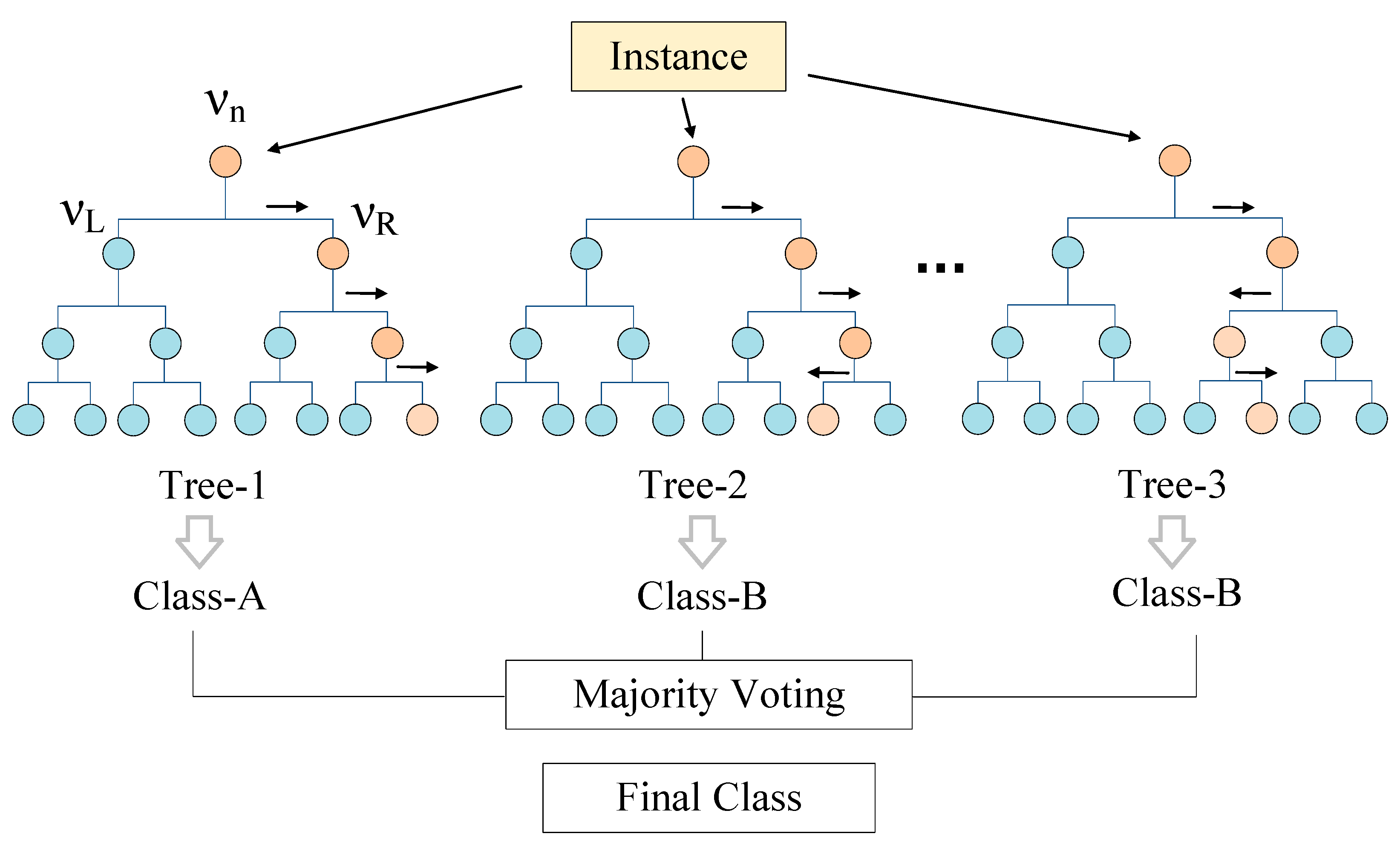
Figure 3 illustrates the process of RF classification with N trees. Starts from the root node νn, samples are passed to the right node (νR) or the left node (νL) after comparing with some criteria or threshold values. Repeat this partition until reaching a terminal node and get a classification label (classes A or B in this case). For classification problem, the ensemble prediction is obtained as a combination of the results of the individual trees by majority voting rule [56].
RF combines all the generated decision trees by a method called ‘bagging’ or ‘bootstrap aggregation’ to decrease the variance of model. The main idea of bagging/ bootstrap is to train several different models from randomly sampling feature subset or training data subset separately, and then let all models vote on the output of the test samples. Bootstrap is a sampling method with replacement. For acquiring a bootstrap sample, it randomly selects a subset of observations from the complementary set Sn. Therefore, the probability of each observation to be picked is 1/n.
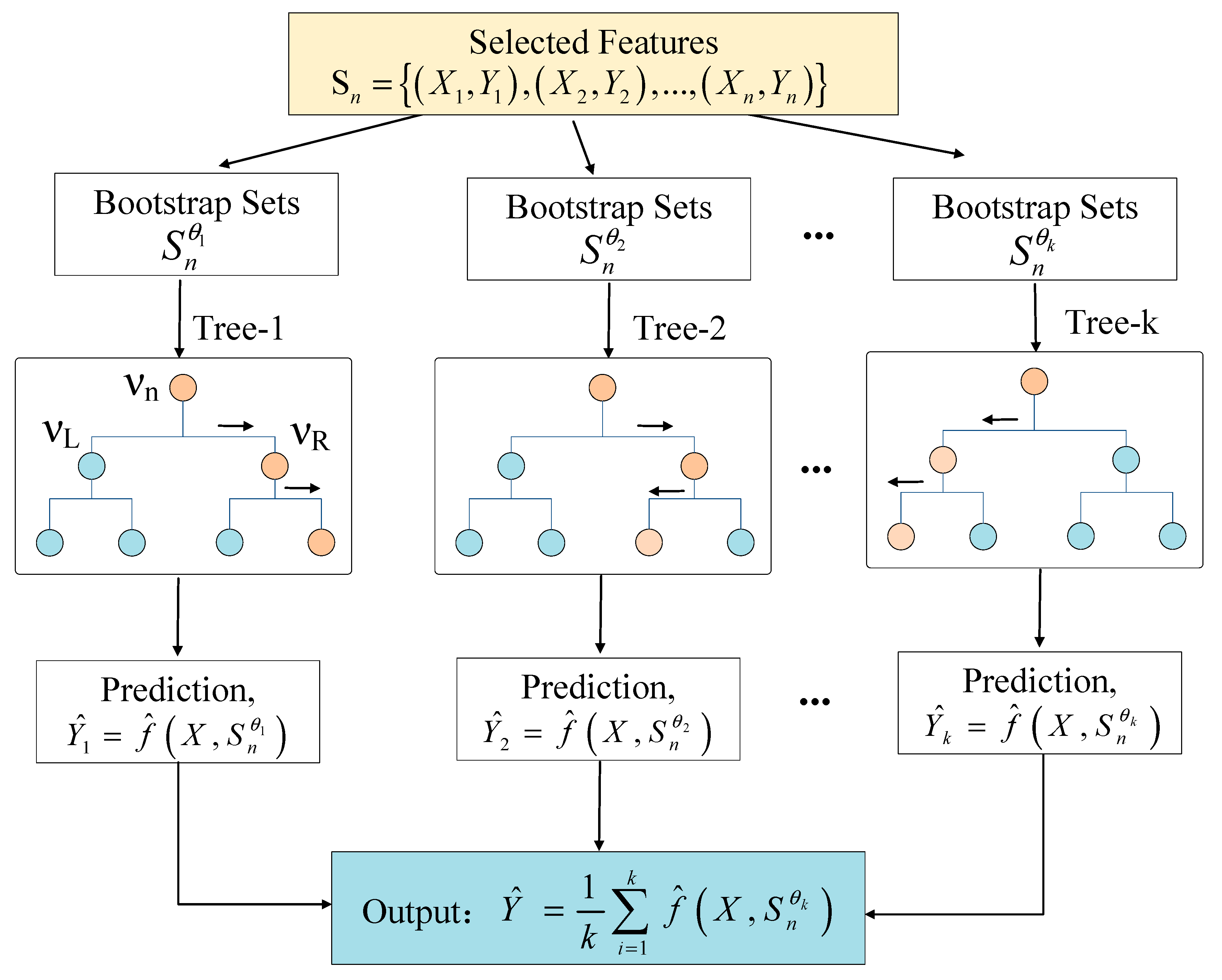
First, RF uses bagging algorithm to generate several bootstrap samples . Second, k prediction trees ,…, are constructed and the RF is built from these collection of trees. The predictions corresponding to each tree from the previous tree decision algorithm are ,…, . The ensemble prediction given by entire forest is obtained as a combination of the results from k trees. Therefore, for regression problem, the estimation of can be calculated as:
where is the prediction of i-th tree, and i = 1, 2, …, k. The framework of using RF regression for prediction is illustrated in Figure 4.
Usually, RF uses the Residual Sum Squares (RSS = ) as split criteria in regression. The optimization process tries to find the split that maximizes the RSS between-groups in an analysis of variance [57]. The relative importance of input features of a RF model can be evaluated by collecting each feature’s contribution from the prediction trees in the model. A higher value of this metric, compared to another, implies greater importance of such feature for generating a prediction.
2.4. XGBoost Algorithm
XGBoost (eXtreme Gradient Boost), proposed by Chen et al. [58], is an integrated machine learning algorithm based on decision tree. Recently, XGBoost has been one of the most widely used methods in Kaggle’s data science contest. It possesses many outstanding properties, including high efficiency and promising prediction accuracy [40,41]. Essentially, XGBoost can be regarded as an improved GBDT (Gradient Boosting Decision Tree) algorithm, because they are all composed of multiple decision trees. Nowadays, XGBoost is widely used in many areas, such as data science competitions and industry, because it has the following advantages:
(1) Many strategies are used to prevent overfitting, including normalization in the objective function, shrinkage and column subsampling.
(2) Second-order Taylor expansion is applied to the loss function, which can make the gradient convergence faster and more accurate.
(3) The parallel computing is implemented in the process of node splitting, which improves the speed of calculation effectively.
(4) The techniques for handling of missing/sparse data, cross-validation and early stop in building trees, all of which can contribute to higher speed and accuracy.
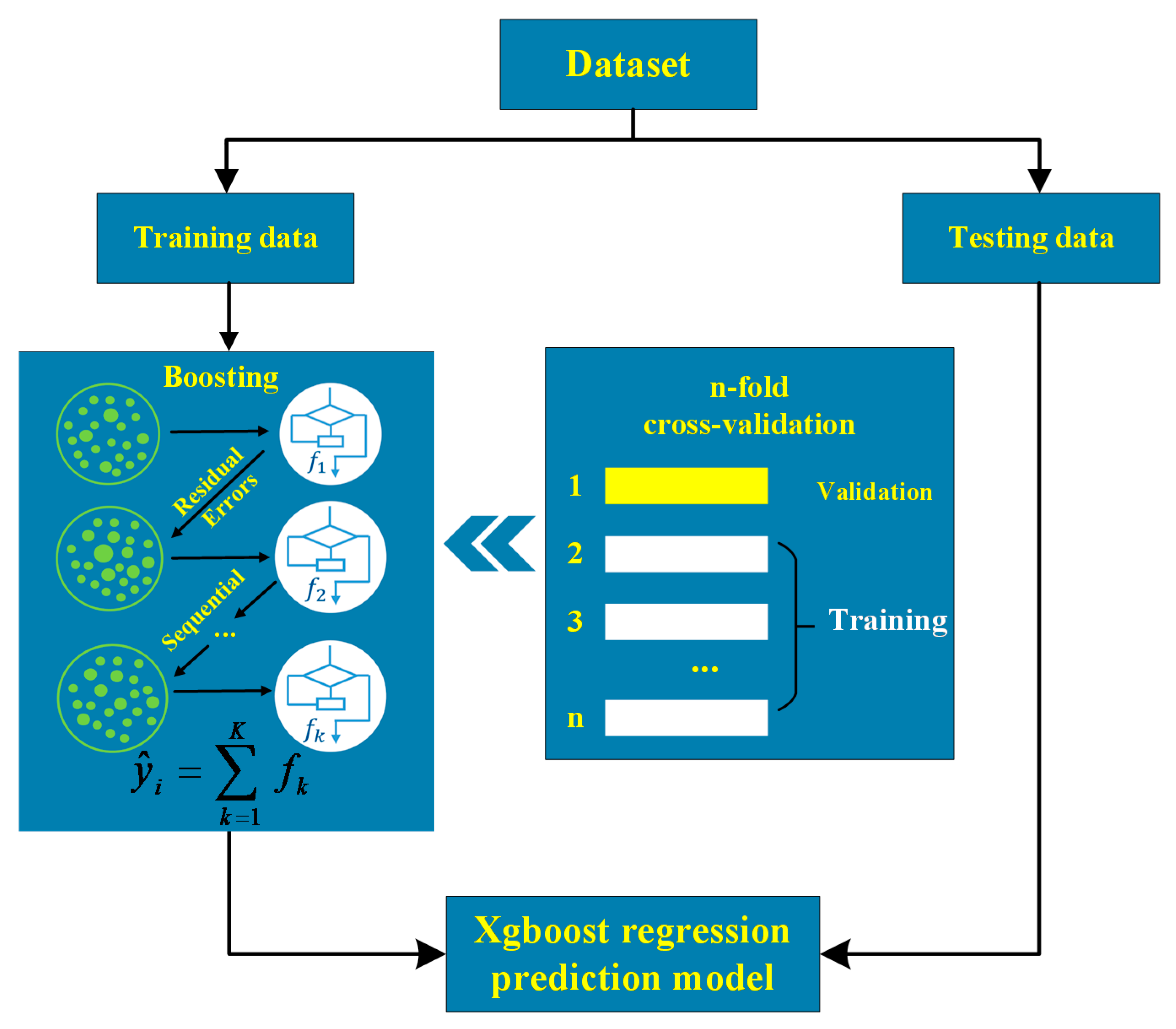
The schematic of XGBoost algorithm is illustrated in Figure 5. XGBoost constructs decision trees one after one so that each successor tree is built to minimize errors in the previous tree. Therefore, the next tree in the sequence will try to decrease the updated residual from the previous tree. Considering a model with k trees finishes training in the dataset , the output of the model should be:
In which f(x) is a regression tree, K is the total number of trees, k represents the kth tree, xi is the input variable corresponding to sample i, corresponds to the predicted score from this tree, and F is the space of regression trees.
XGBoost’s objective function includes two parts: the training error and the regularization:
where L(.) is the loss function quantifying the deviation of the predicted values from the actual values. Ω (fk) is the regularization function penalizes the complexity of the model from overfitting:
In which T represents the total number of leaf nodes, and is the score of each leaf node. and are the controlling factors employed to avoid overfitting. indicates the complexity cost by introducing additional leaf. evaluates the performance of a decision tree. Therefore, this objective function tends to choose a simple predictive function from candidate models.
When a new tree is created to fit residual errors of last iteration, the prediction for the tth tree can be expressed as:
In which is the prediction of the ith instance at the tth iteration. Therefore, the objective function can be expressed as:
Then, the objective function is approximated by the second-order Taylor expansion as:
where and are first and second order gradient statistics of the loss function, respectively:
Because the previous (t−1) trees’ residual errors have minimal influence on the modification of the objective function, an approximation in step t can be:
Then, the tth tree concerning the model parameters and predictions can be determined by optimization of Equation (16). In the same way, the successor trees are built until the whole XGBoost is constructed satisfying predefined finishing standards [58]. The input feature importance of a XGBoost model can be evaluated through the gain criterion. The gain is obtained by collecting each feature’s contribution from each tree in the model. A feature with higher value indicates greater relative contribution and importance.
2.5. MARS Methodology
Friedman [59] presented a Multivariate Adaptive Regression Splines model (MARS) as a flexible regression method for modeling of high dimensional data. MARS has become particularly popular in the area of data mining because it does not assume any particular type or class of relationship between the predictor variables and the outcome variable. MARS partitions the training data sets into continuous regions and tries to fit the data in each region with separate piecewise linear segments (splines) of differing gradients (slope). The endpoints of the segments are called knots. A knot marks the end of one region of data and the beginning of another. The resulting piecewise linear segments (known as basis functions), give greater flexibility to the model, allowing for bends, thresholds, and other departures from linear functions.
Let y be the target output and X = (X1, …, XP) be a matrix of P input variables. In case of a continuous response, this would be:
In which e is the distribution of the error. MARS approximates the function f by applying basis functions (BFs). BFs are splines (smooth polynomials), including piecewise linear and piecewise cubic functions. For simplicity, only the piecewise linear function is expressed here. Piecewise linear functions in MARS are of the form with a knot occurring at value a as:
The MARS model f(X) is constructed as a linear combination of BFs as:
where each λm (X) is a basis function. It can be a spline function, or the product of two or more spline functions already contained in the model. The coefficients β are constants estimated using the least-squares method.
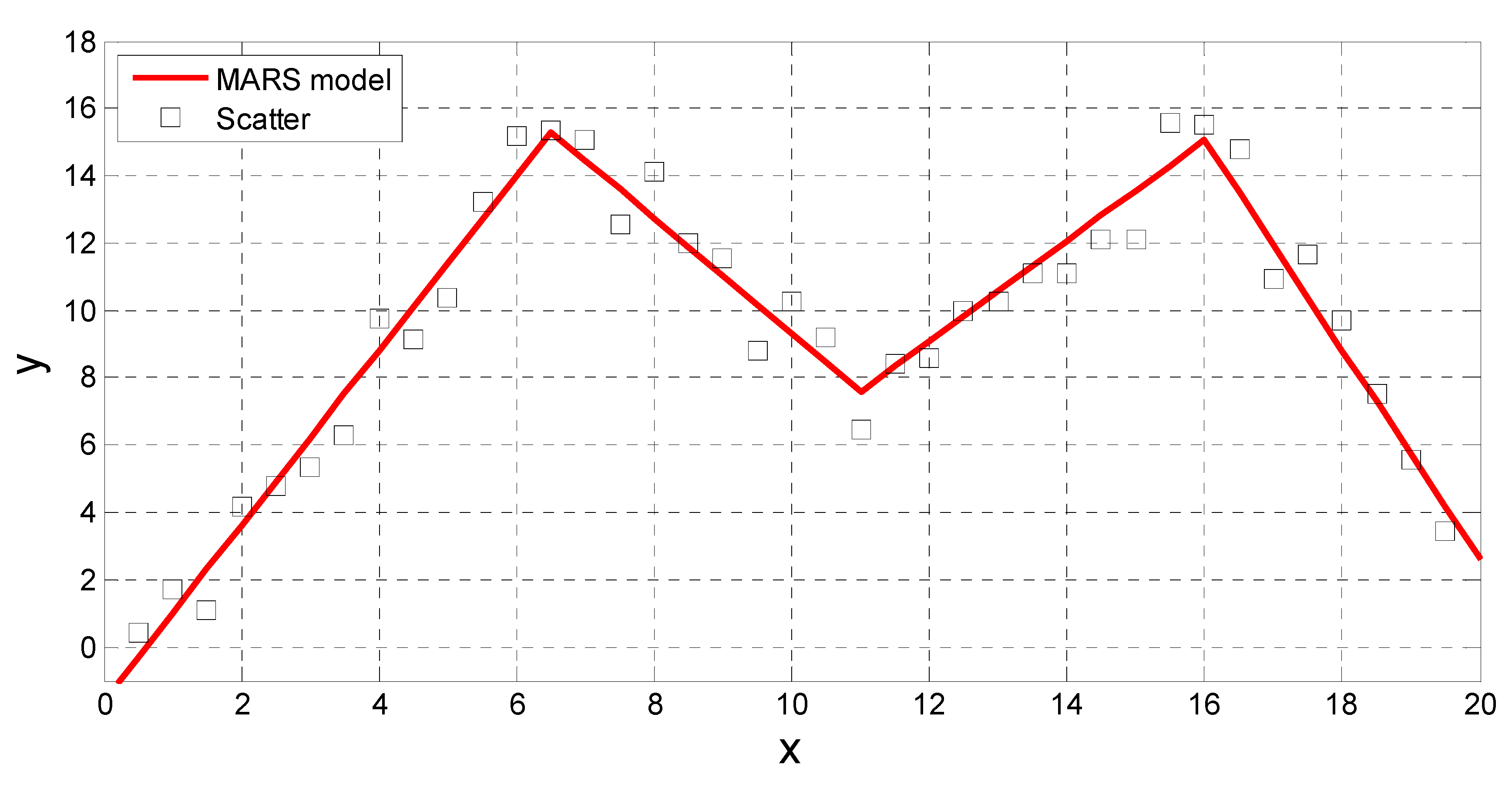
Figure 6 shows a simple example of how MARS would use piecewise linear spline functions to attempt to fit data. The MARS mathematical equation is expressed as:
where BF1 = max(0, 16−x), BF2 = max(0, x−11), BF3 = max(0, x−6.5), and BF4 = max(0,6.5−x). The knots are located at x = 6.5, 11 and 16. They define four intervals with different linear relationships.
In general, MARS follows three basic steps to fit the model in Equation (19):
(i) Constructive phase (forward phase). The intercept and the basis functions that generate the maximum training error decrease are added to the Model. For a current model with M basis functions, the following terms to be added can take the form of:
In which the coefficients β can be obtained through the method of least squares.
Stop adding BFs when the model has more terms than a predefined number in order to construct an overfit model intentionally.
(ii) Pruning phase (backward phase). The least significant BFs that does not meet the standard of contribution is removed to find an optimal submodel. Candidate models are compared by the computationally effective method of Generalized Cross-Validation (GCV). GCV reduces the chance of overfitting by penalizing the model with large numbers of BFs. Hastie et al. [60] gave the formula to calculate the GCV for a MARS model as:
In which N is the number of observations in the training set, M is the number of BFs, and denotes the predicted values of the MARS model. The numerator is the mean squared error (MSE) of a candidate model. The denominator takes into account the larger uncertainty with increasing model complexity. d is the penalizing parameter with a default value of 3 [59]. The GCV can penalize both the error of the model, the number of BFs and number of knots. At each step in the pruning phase, an extraneous BF is removed to minimize the error of the model until a satisfactory model is gained.
(iii) Selection of optimum MARS.
MARS has great flexibility and adaptability because the basic functions and the knot locations are automatically determined by the data. Previous applications of MARS algorithm in civil engineering can be found in the recent works [26,27,28,29,30,31,32,33,34,35,36,37,38,39,40,41,61,62,63,64,65].
As long as the final MARS model is constructed, the method known as analysis of variance (ANOVA) decomposition (Friedman, 1991) [59] can be utilized to evaluate the contributions from the input variables and the BFs through comparing (testing) variables for statistical significance. This is done by collecting together all the BFs that involve one variable and another grouping of BFs that involve pairwise interactions.
2.6. Performance Measures
Assessments of the performance of models are evaluated according to the performance measures. In the following equations, is the mean of the target values of , is the mean of the predicted , and N is the total number of data points in the training set or testing set.
The root mean square error (RMSE) evaluates the errors between prediction values and true values as [66]:
The mean absolute error (MAE) is the average of absolute errors of predictions, calculated as:
The coefficient of determination R2 (R2) measures the deviation of a group of data and characterizes the goodness of regression fitting [67]:
3. Models for Soil Liquefaction Assessment Based on Capacity Energy Concept
3.1. The Database
The database used for modeling comprises of 271 cyclic triaxial tests, 116 cyclic torsional shear tests, and 18 cyclic simple shear tests giving a total of 405 tests. A summary of the laboratory tests, as well as the parameter statistics, are listed in Table 1. The specific details of the 405 tests, including the test type, values of parameters, and the failure mode, can be found in the studies by Baziar and Jafarian (2007, 2011) [13,19].
Of the 405 data sets, 324 (approximately 80% of the total data sets) were randomly selected as the training patterns while the remaining 81 were used for testing purposes. As the previously proposed regression and soft computing models did not indicate the specific information of the training and testing patterns, for performance comparison, the criterion of data pattern selection used in this study was based on ensuring that the statistical properties, including the mean and standard deviations of the training and testing subsets, were similar to each other.
3.2. Ridge Modeling Results
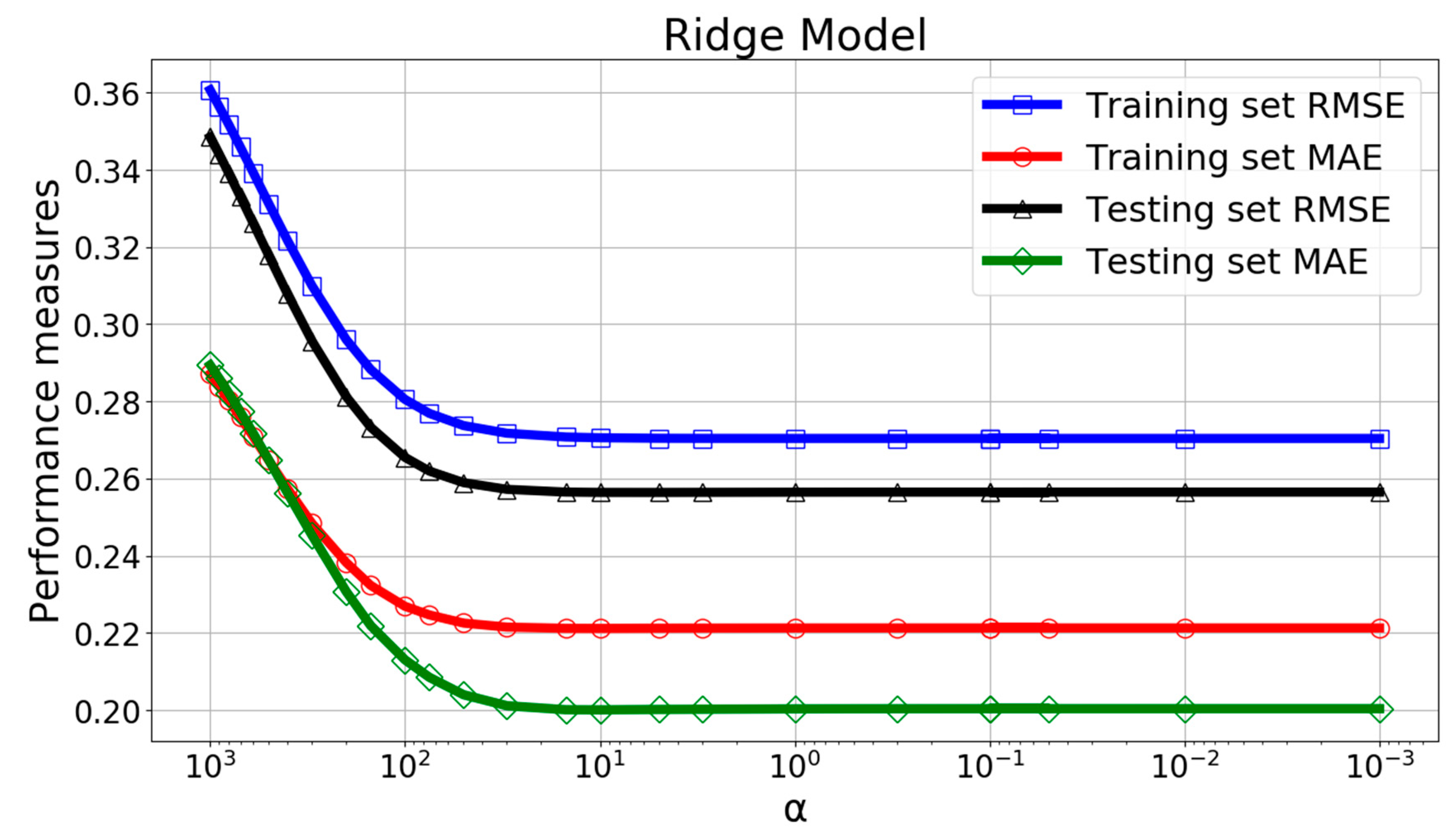
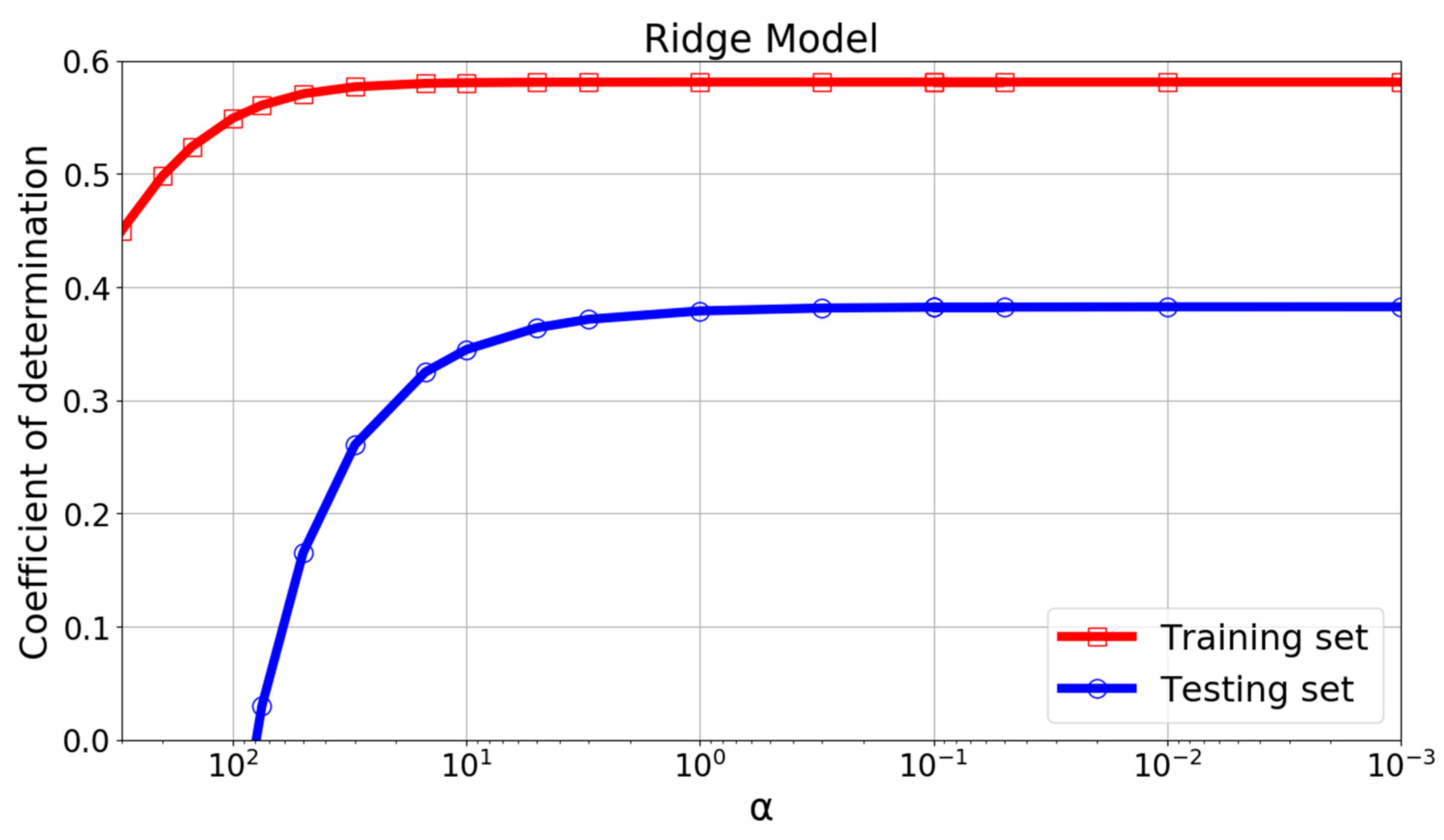
The ridge regression parameter has strong influence on the performance of the model. Figure 7 and Figure 8 shows the variation of performance measures with . It was found that when was between 0.1 and 0.001, the RMSE, MAE, and coefficient of determination curves remained almost constant in both the training and testing set. Therefore, a ridge regression parameter of 0.01 was picked finally.
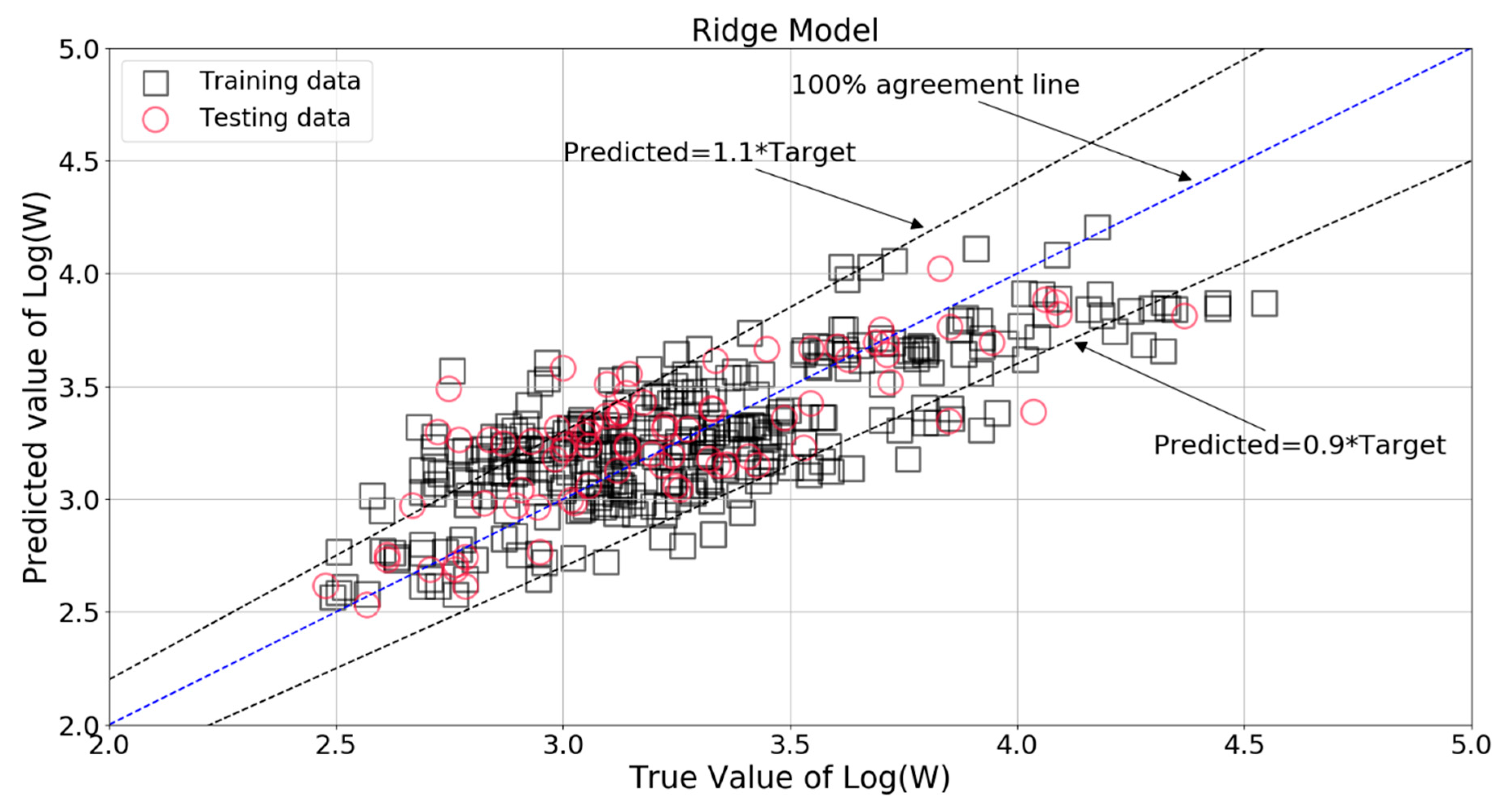
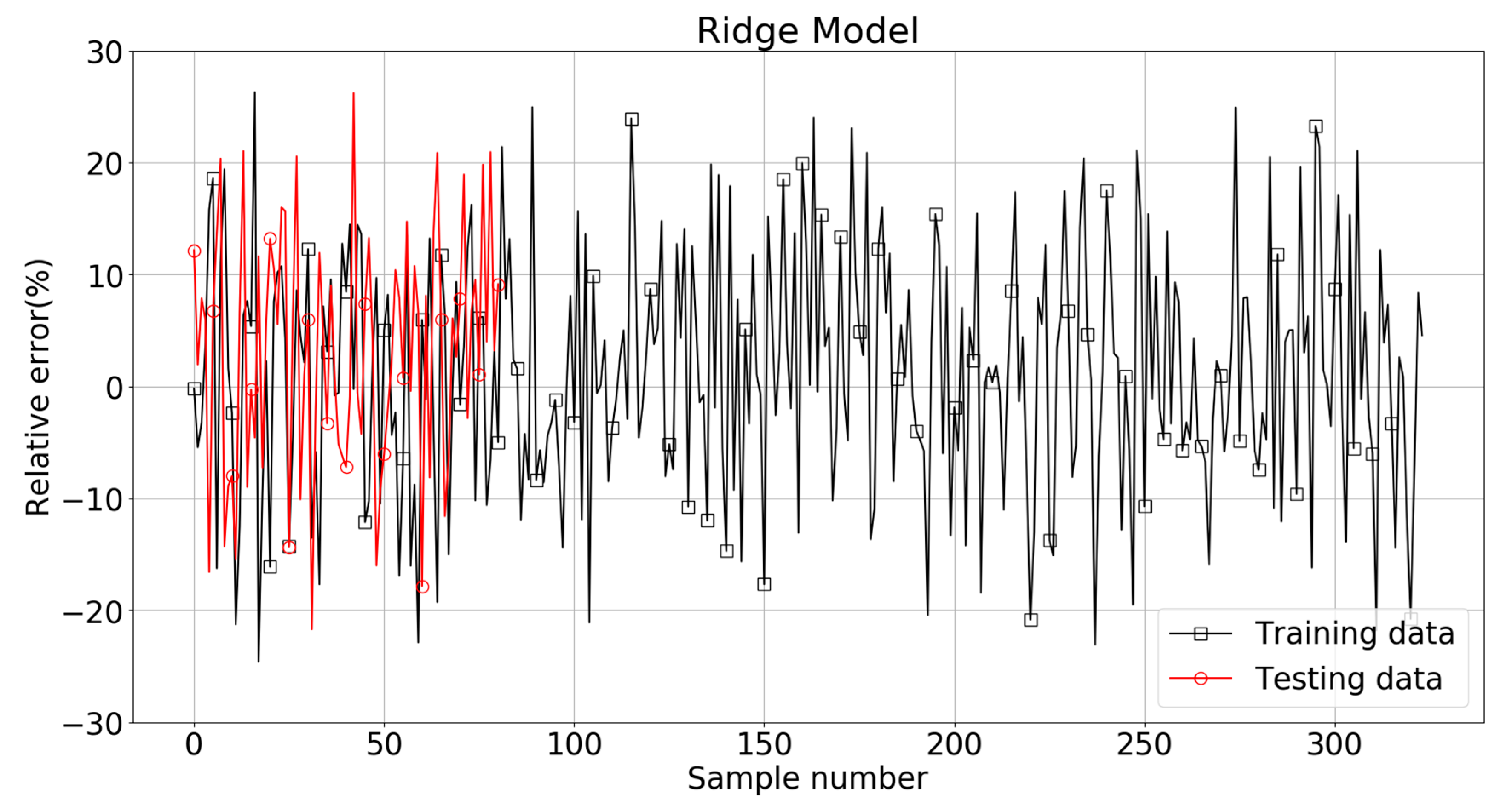
The comparison between the true value and Ridge model predicted value of Log(W) is shown in Figure 9. The main part of the estimations of Log(W) were within ±10% of the target values, but quite a lot of points were still outside these two limit lines. The relative errors (defined as the ratio of the difference between the Ridge predicted and the target Log(W) values divided by the target value, in percentage) for the training and testing patterns are plotted in Figure 10. It can be seen that some relative errors were above 20%. The RMSE, MAE, and R2 scores were 0.271, 0.221, and 0.582 for the training set, with the corresponding scores of 0.258, 0.201, and 0.382 for the testing set. The results show that this model could not provide satisfactory predictions, especially in the testing set.
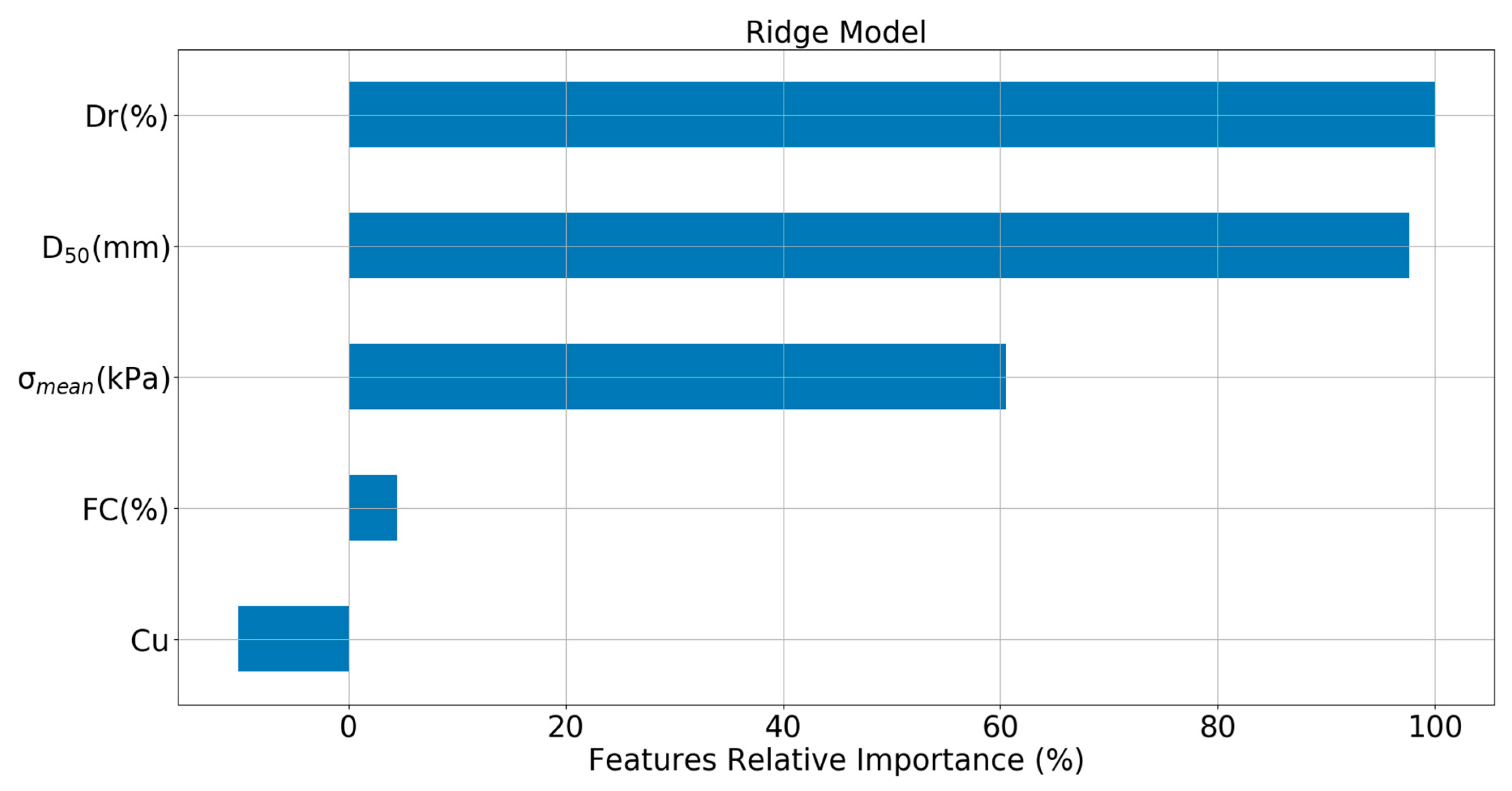
Figure 11 gives the plots of the relative importance of the input variables for the Ridge model, which was evaluated by the regression coefficient. For simplicity, percentage was used to sort the importance scores of the five variables from high to low. It can be seen that Dr was the most important feature variable, followed by D50 and . FC had a very small relative importance index (4.42%), and Cu had a negative importance index of −10.1%.
3.3. Lasso and LassoCV Analysis
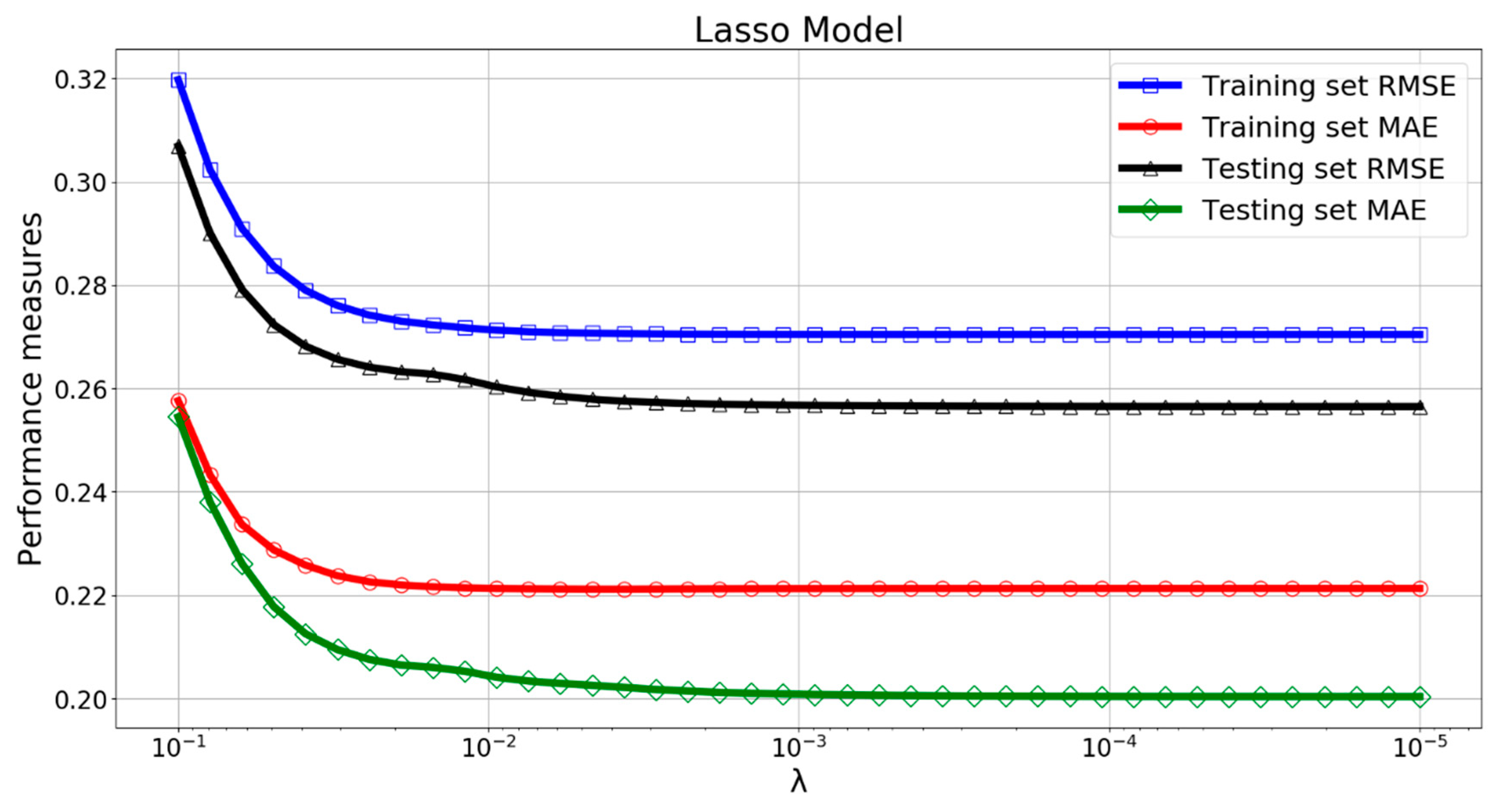
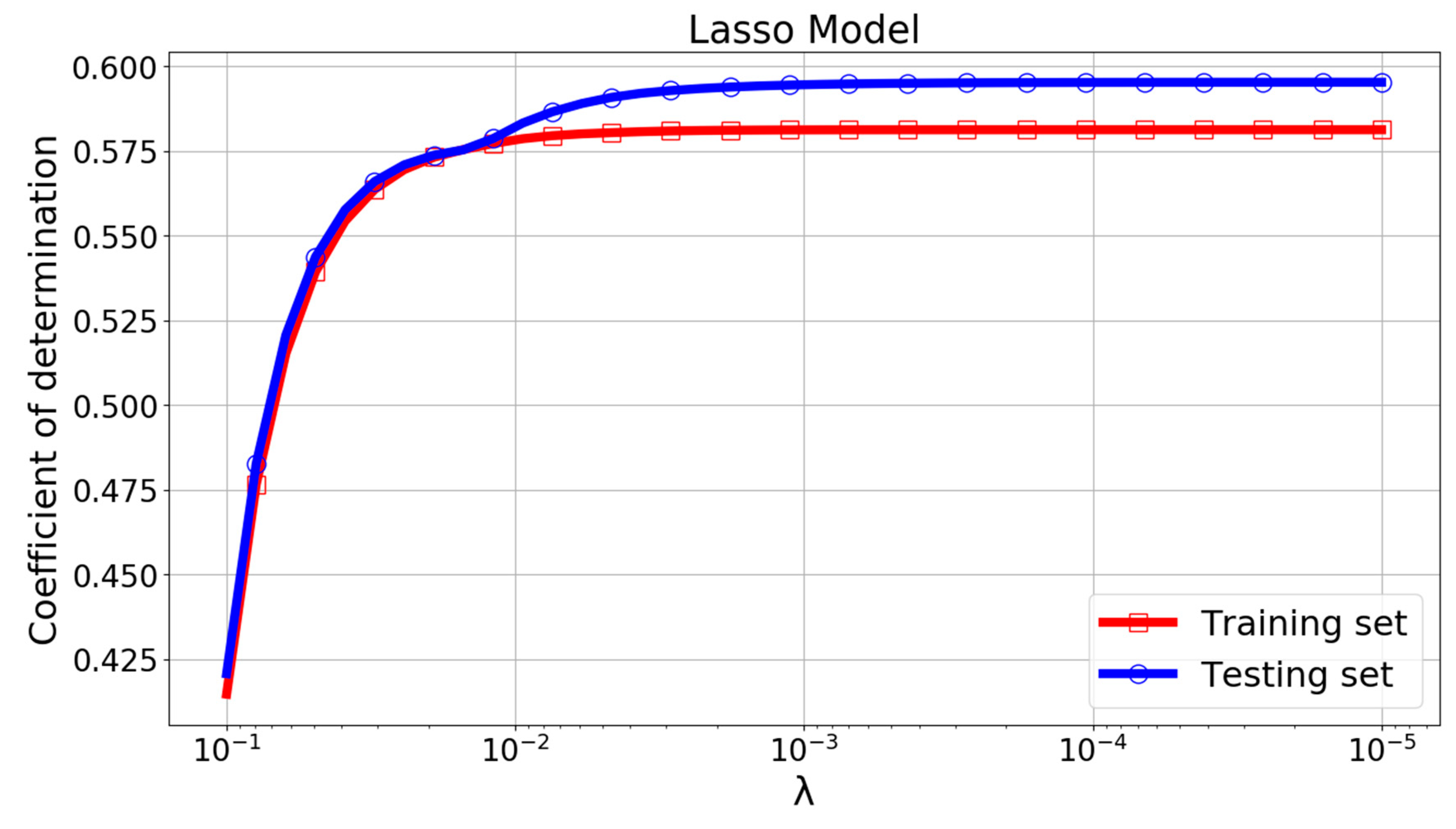
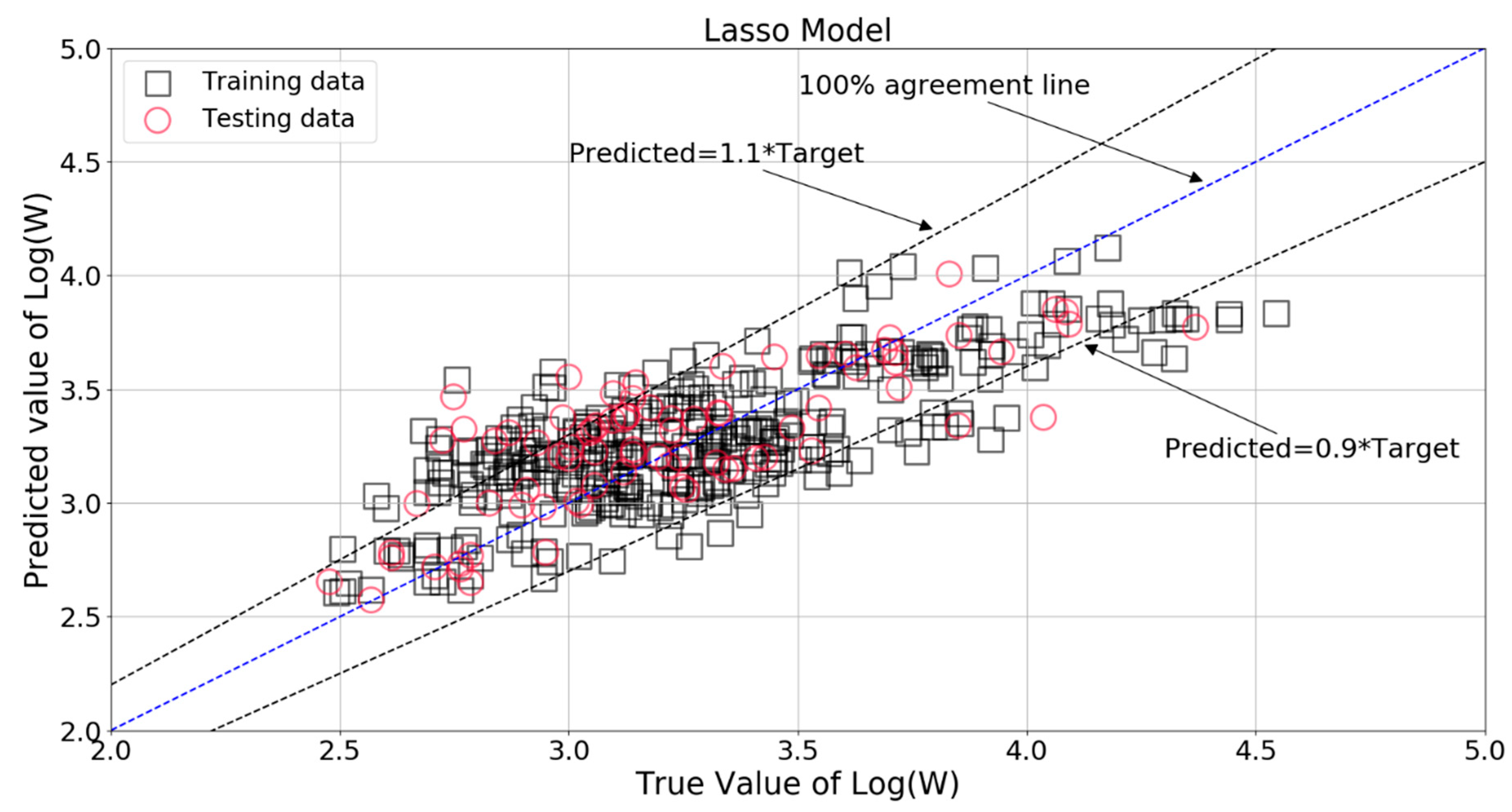
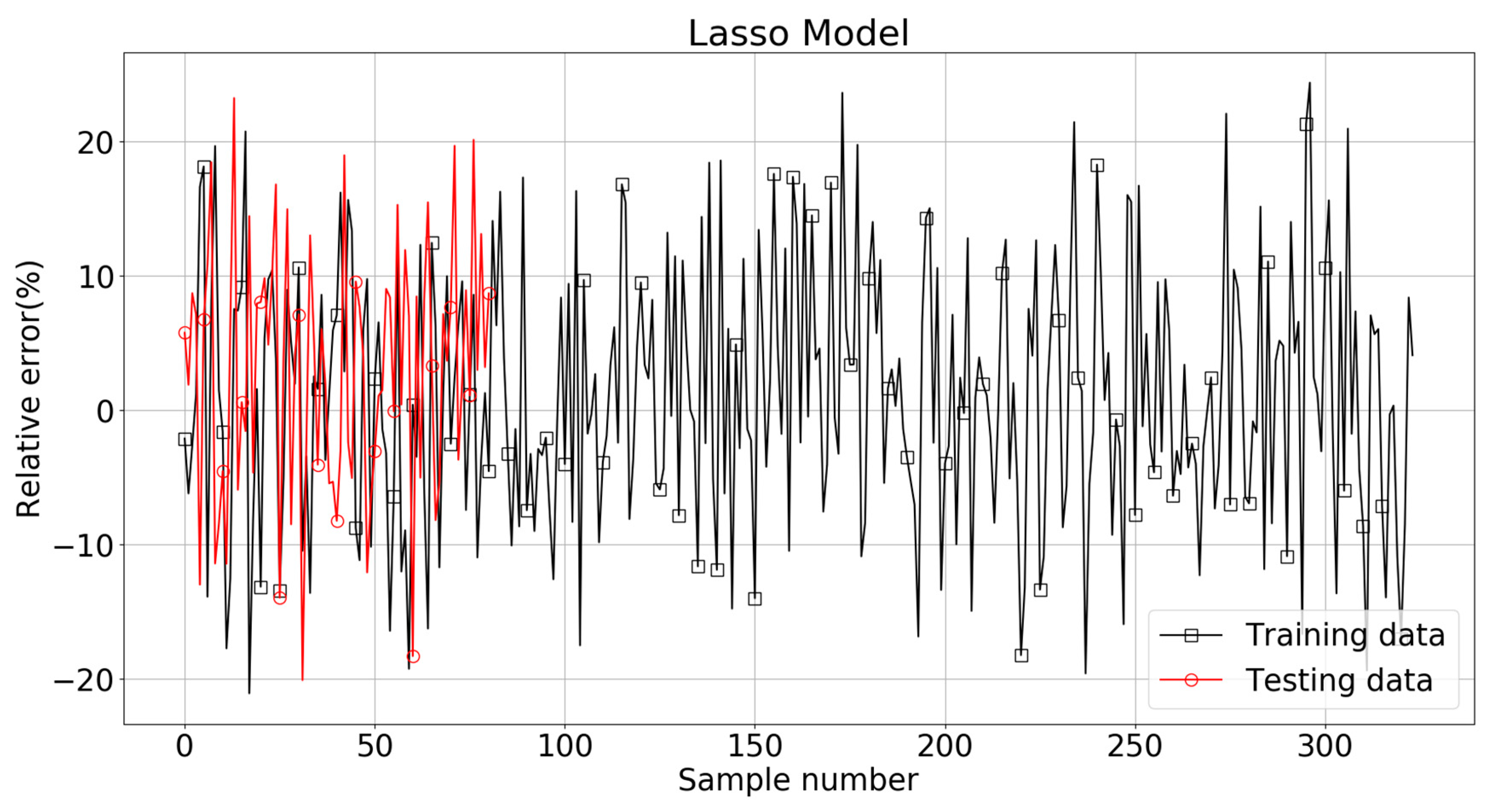
The performance of Lasso model greatly depended on the parameter λ in Equation (6). Figure 12 and Figure 13 shows the variation of performance measures with λ. It can be found that the RMSE, MAE, and R2 curve become constant when λ was smaller than 0.01. The LassoCV algorithm automatically picked 0.001053 as an optimal value of λ. The true value and LassoCV model predicted value of Log(W) are compared in Figure 14. The main part of the estimations of Log(W) were within ±10% of the target values, but quite a few data points were still located outside the limit lines. The relative errors for the training and testing patterns are plotted in Figure 15. It can be seen that some relative errors were above 20%.
It should be noticed that the RMSE, MAE, and R2 scores were 0.275, 0.225, and 0.578 for the training set, with the corresponding scores of 0.255, 0.201, and 0.581 for the testing set. The results show that this model still could not produce reasonable predictions. Its RMSE and MAE were almost the same as that of the Ridge model, although with a R2 score 51.3% higher than that of the Ridge model. This again proves the insufficiency of this linear regression type algorithm in modeling the complex problem of soil liquefaction.
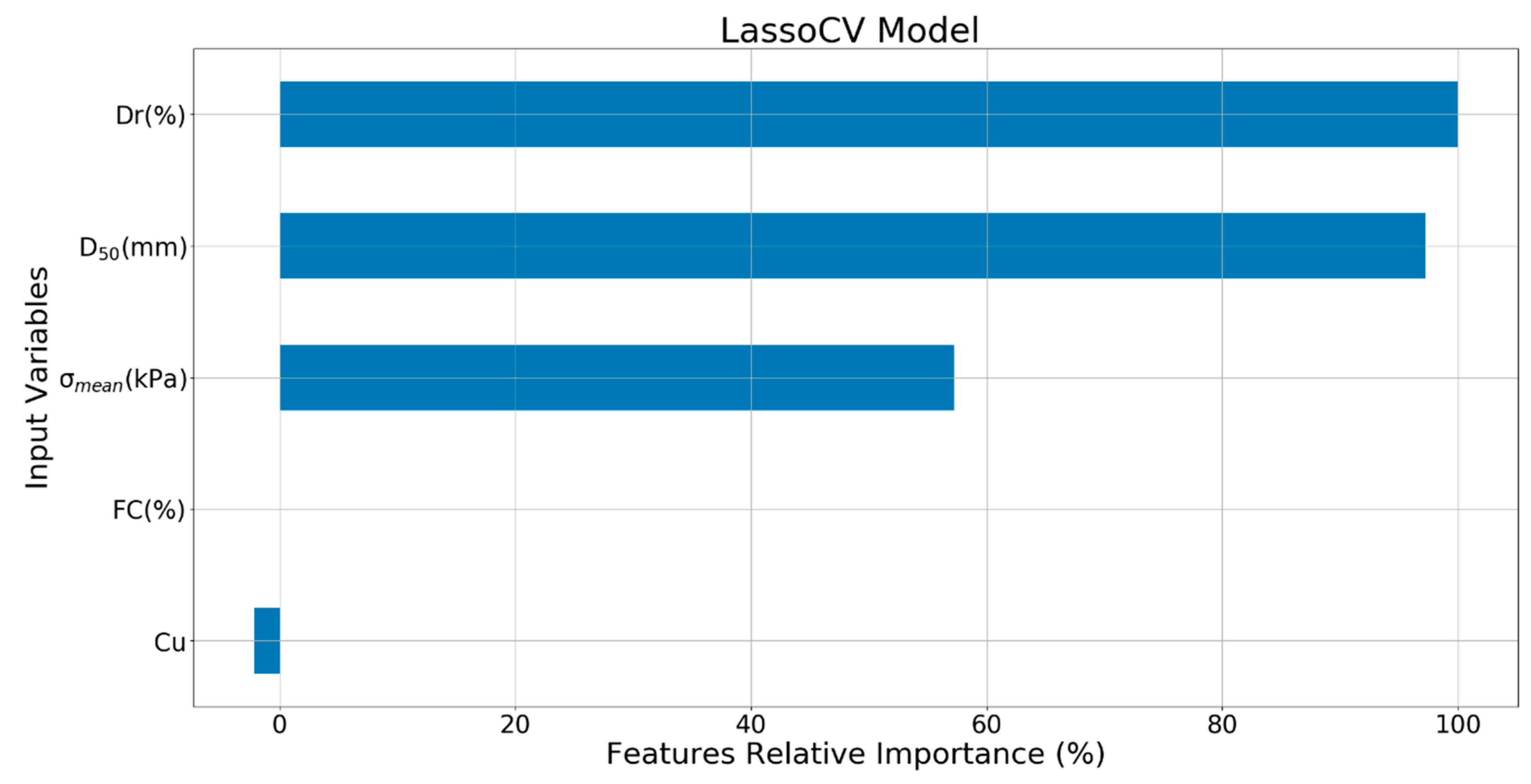
The relative importance of the input variables for Lasso & LassoCV are shown in Figure 16. It can be seen that Dr was the most important feature variable, followed by D50 and . FC was automatically removed by the LassoCV algorithm by having a zero-regression coefficient. Cu had a negative importance index of −2.2%.
3.4. RF Modeling Result
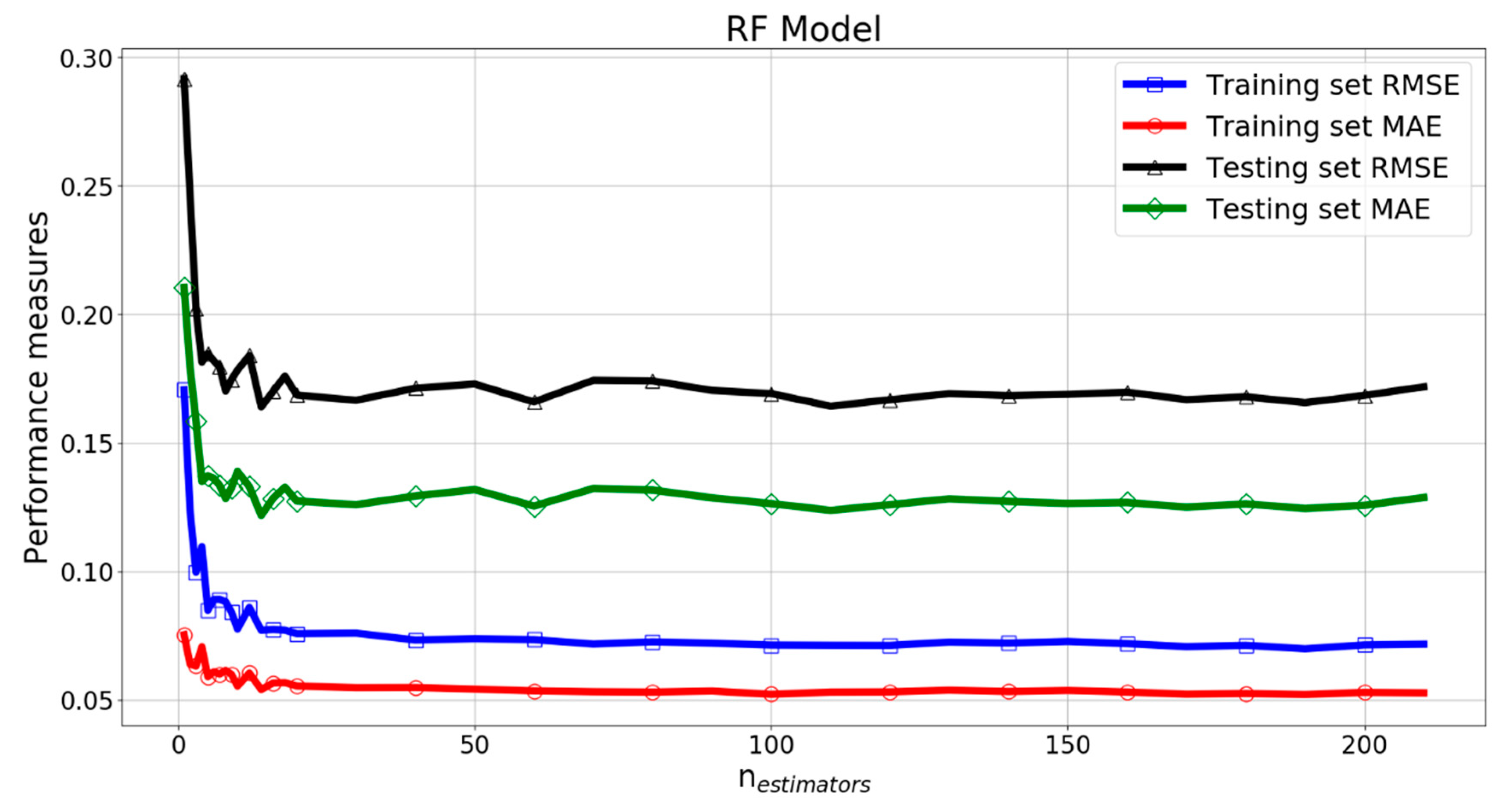
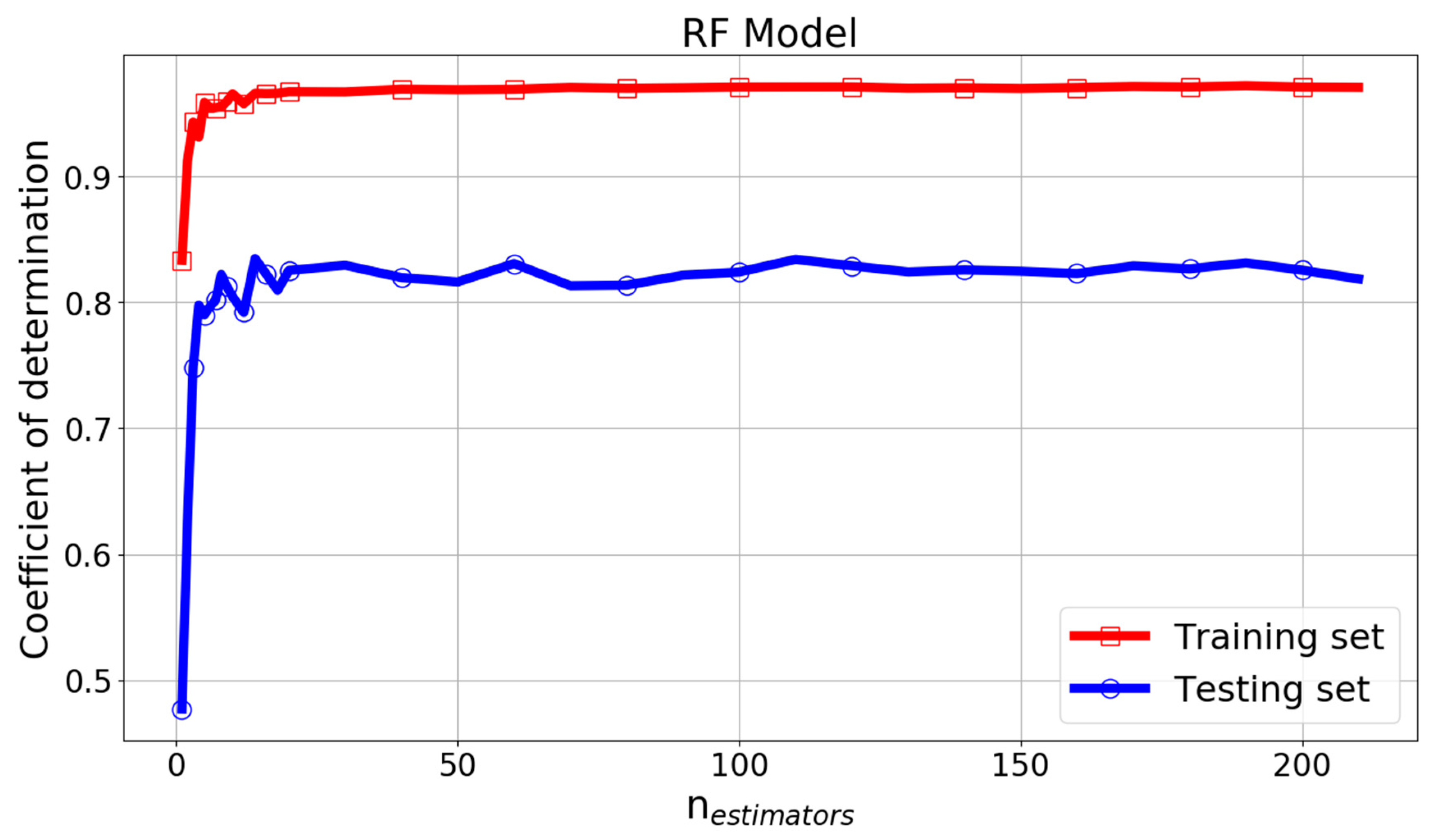
The parameter nestimators is related to the number of decision trees in the RF model. Figure 17 and Figure 18 give the RMSE, MAE, and R2 change curves of RF model with parameter nestimators. It can be seen that when nestimators was greater than 100, the curves of performance measures had only minor fluctuations.
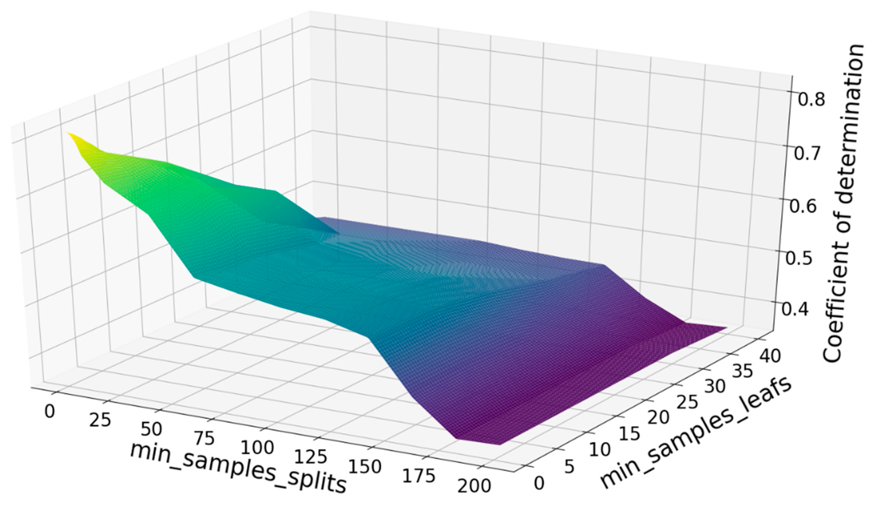
The other two important parameters for the RF model are min_samples_split and min_samples_leaf. The min_samples_split limits the conditions for the subtree to continue to be partitioned. If the number of samples in a node is less than min_samples_split, it will not continue to try to select the optimal feature to partition. The min_samples_leaf limits the minimum number of samples of leaf nodes. If the number of leaf nodes is smaller than the number of samples, it will be pruned together with the sibling nodes. It can be found that the R2 score reaches the maximum value when min_samples_split equals 2 and min_samples_split equals 1, as shown in Figure 19.
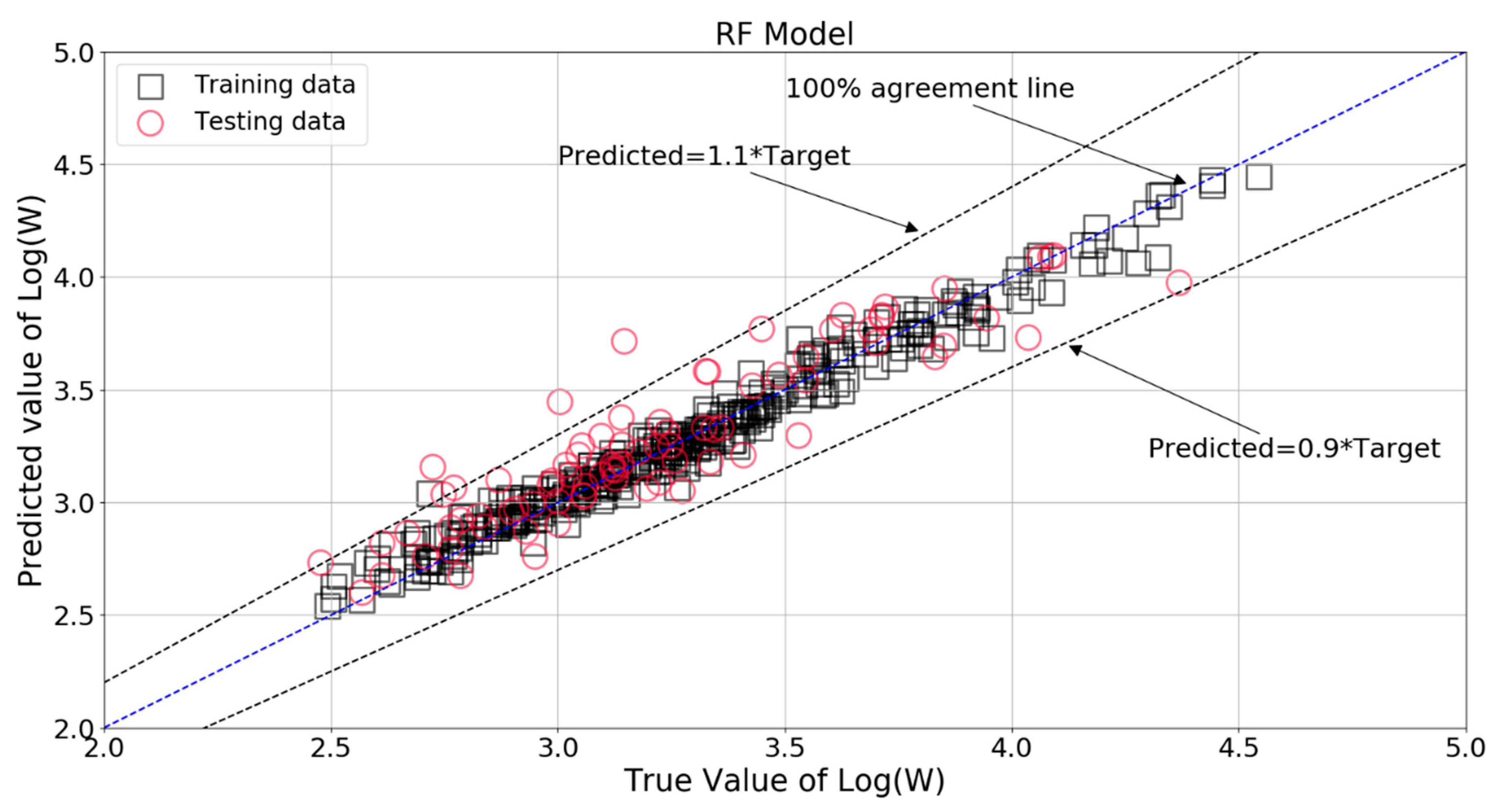
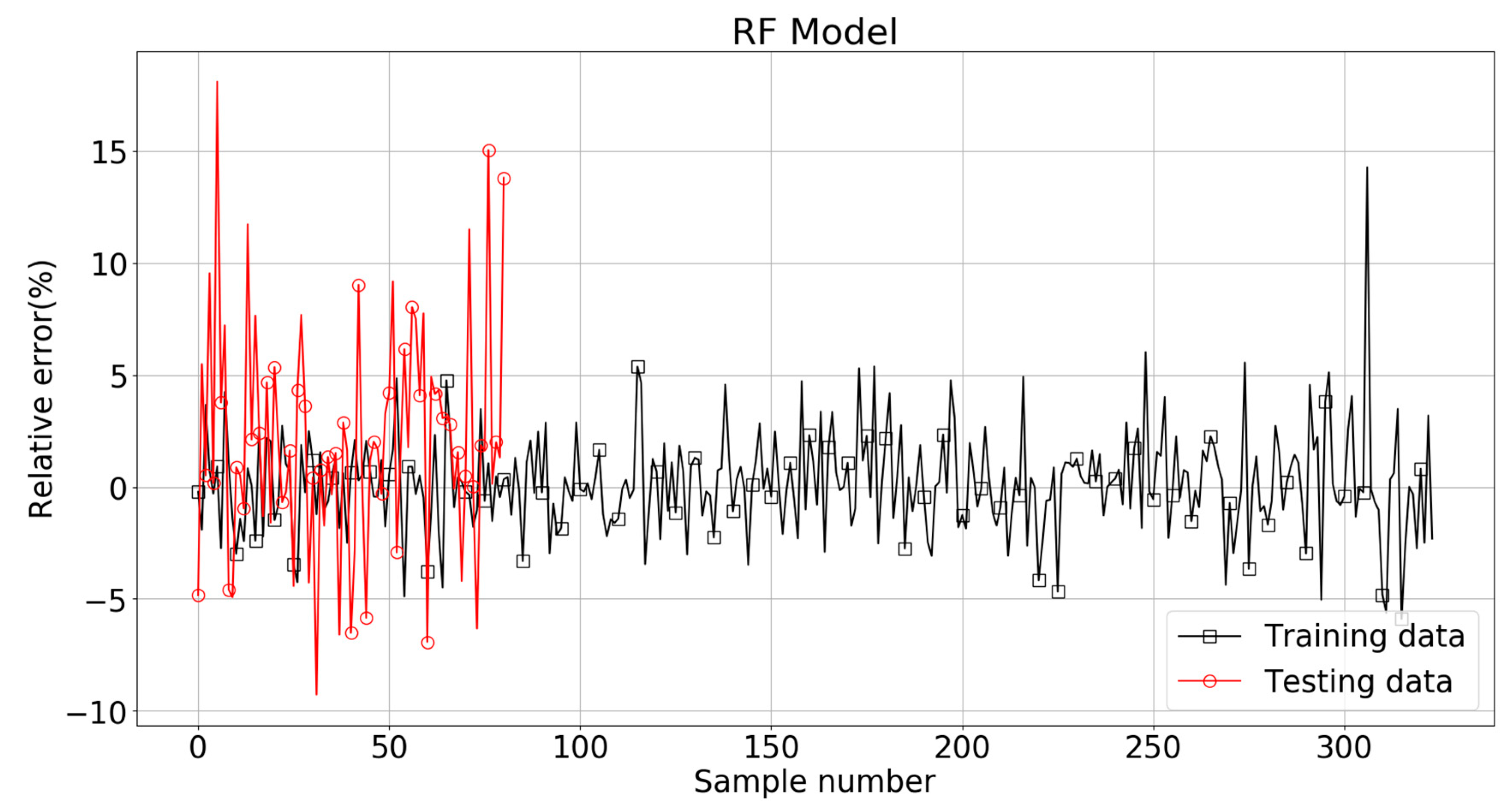
With these optimal pamaters, the comparison between true value and RF model predicted value of Log(W) is shown in Figure 20. It can be seen that almost all the data points of the training set were located in the 100% agreement line, and majority of the testing set data were within ±10% of the target values. The relative errors for the training and testing patterns are plotted in Figure 21. Almost all of the RF estimations of the training set data fell within ± 5% of the target values, and most of the predictions of the testing data were within −5% to +10% of the target values.
It should be noticed that the RMSE, MAE, and R2 scores were 0.075, 0.052, and 0.97 for the training set, with the corresponding scores of 0.175, 0.124, and 0.82 for the testing set. The lower RMSE/MAE and large R2 scores indicate a higher fitting performance than the Ridge model and Lasso model.
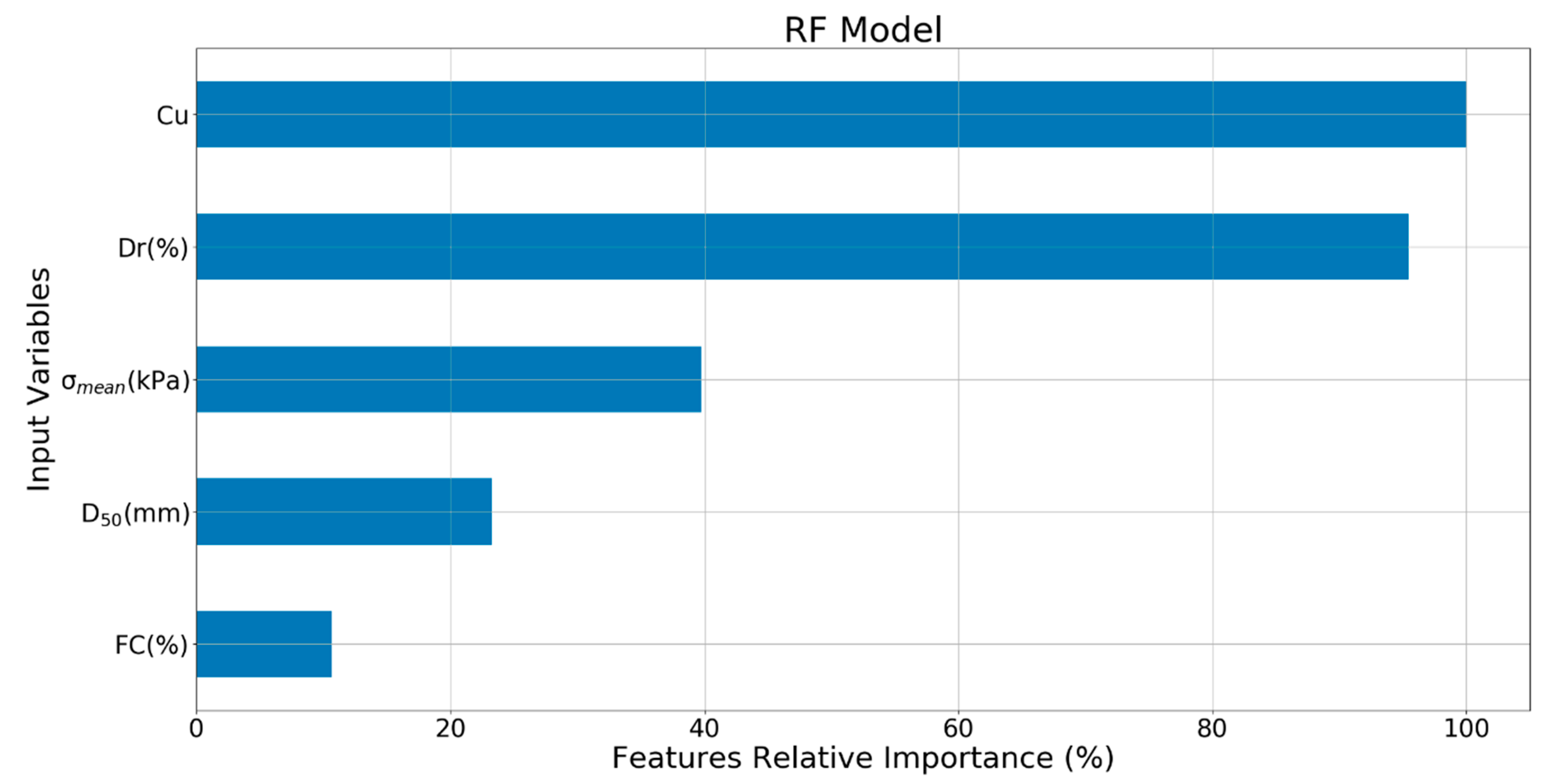
The relative importance of the input variables for RF model is plotted in Figure 22. It can be seen that Cu and Dr were the most important two feature variables, followed by , D50, and FC.
3.5. XGBoost Modeling Result
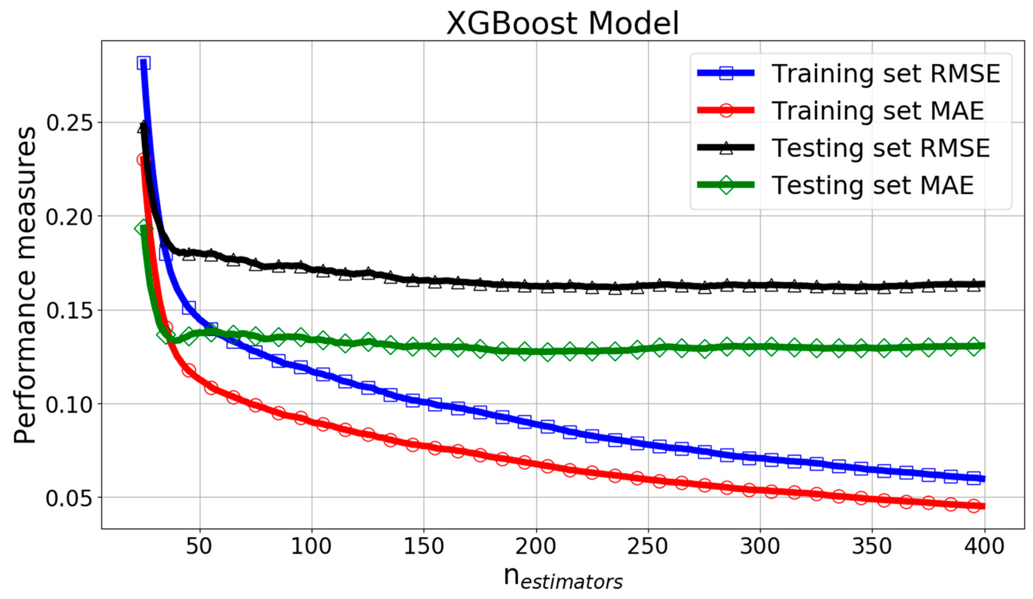
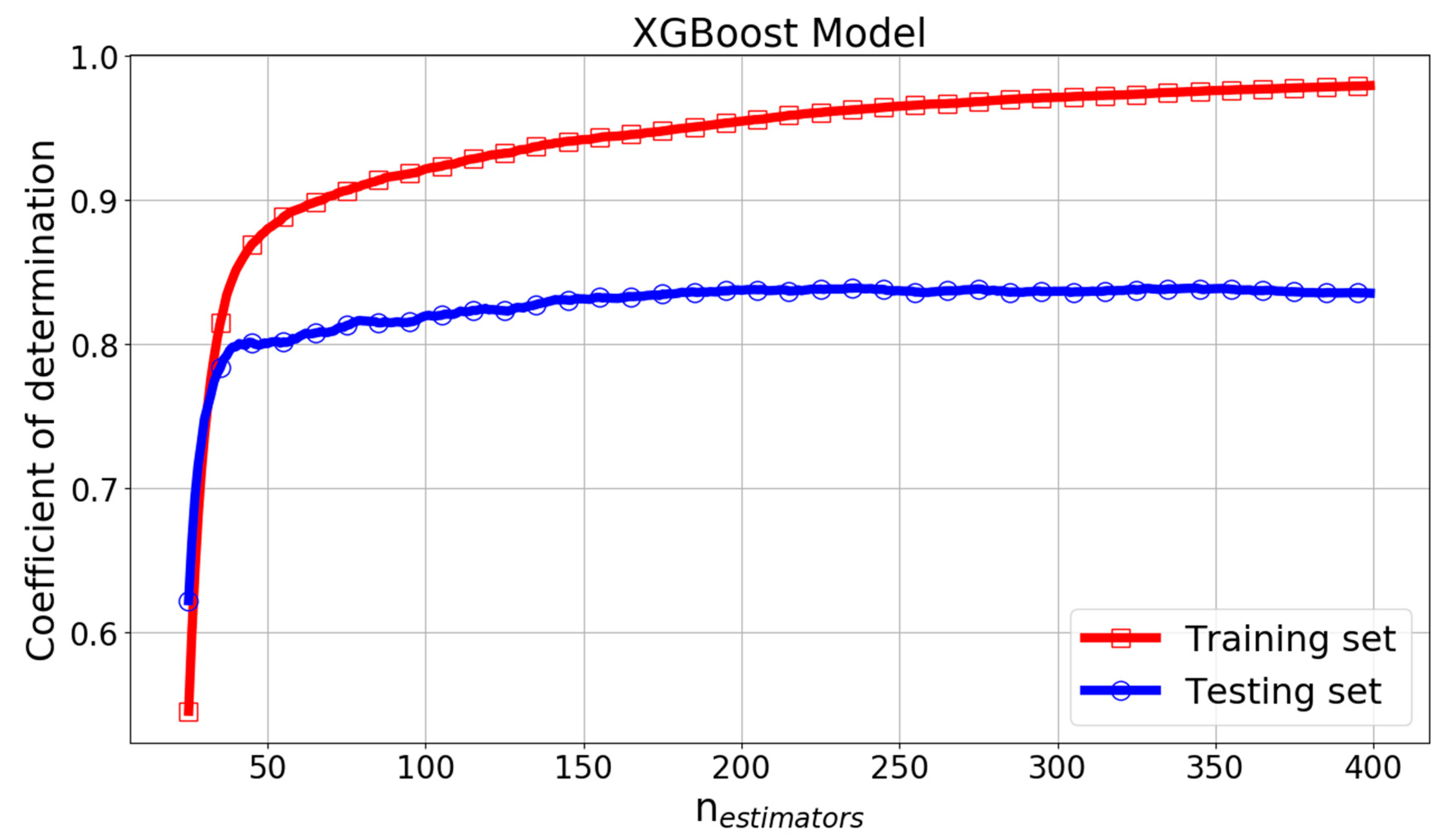
In the XGBoost model, the most important parameter is nestimators, which controls the number of decision trees. Figure 23 and Figure 24 give the RMSE, MAE, and R2 change curves of XGBoost model with parameter nestimators. It can be seen that for the training set, when nestimators increased, RMSE and MAE decreased and the R2 score increased. However, for the testing set, when nestimators was greater than 200, the curves of performance measures had only minor fluctuations. The optimal nestimators was chosen as 352.
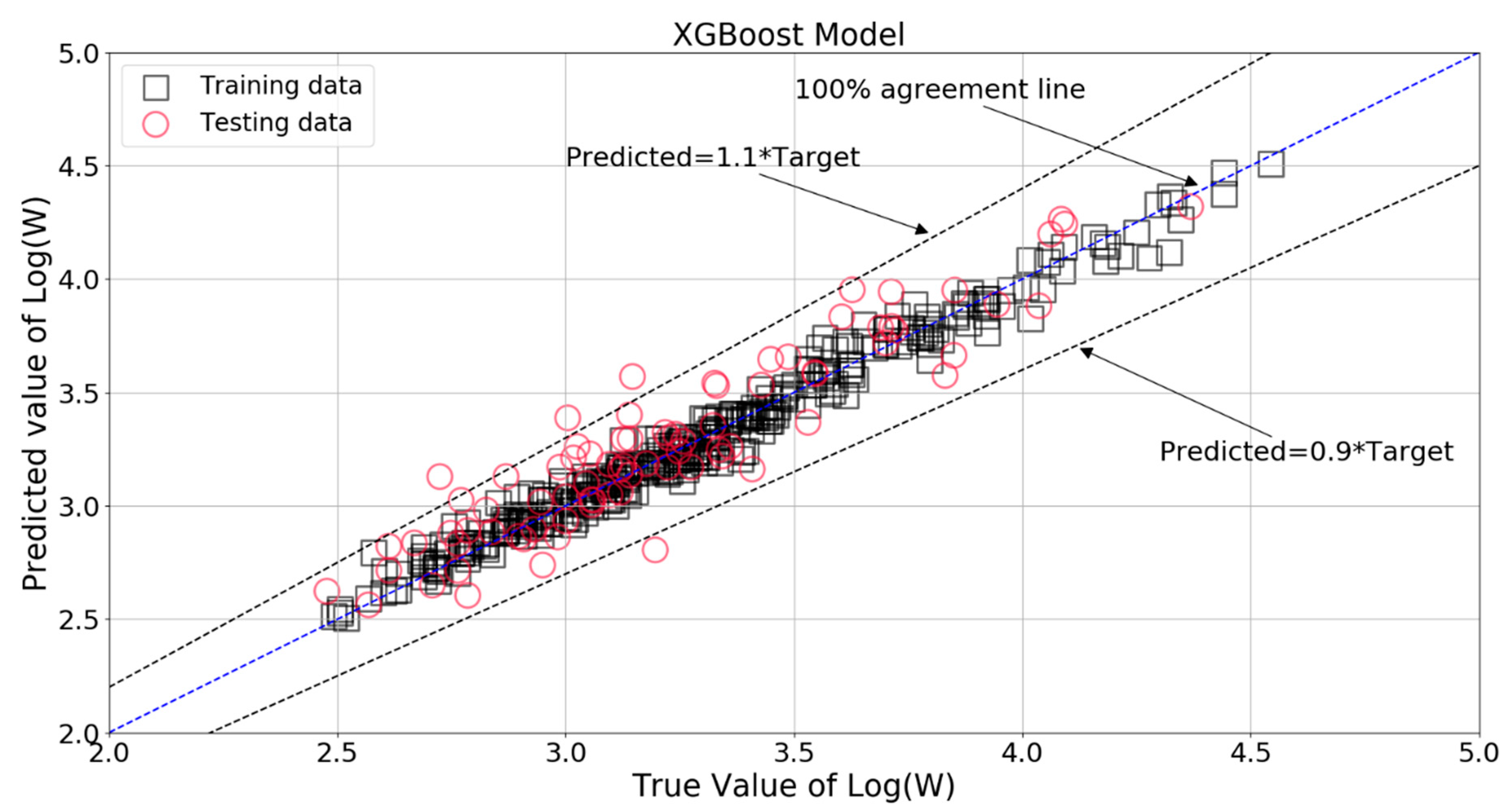
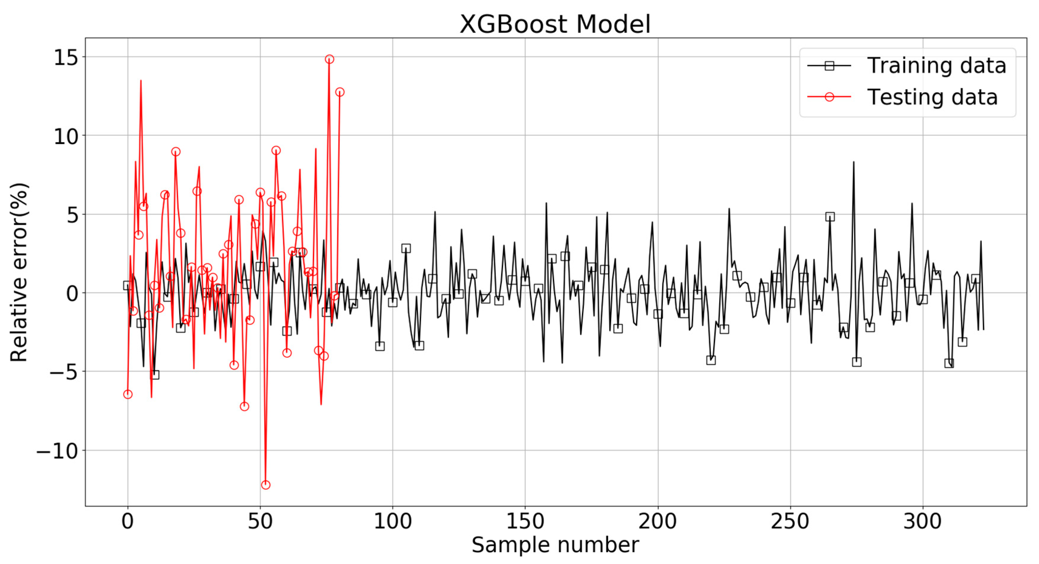
Figure 25 shows the comparison between true value and XGBoost model predicted value of Log(W). It can be seen that almost all the data points of the training set were located in the 100% agreement line, and majority of the testing set data were within ±10% of the target values. The relative errors for the training and testing patterns are plotted in Figure 26. Almost all of the XGBoost estimations of the training set data fell within ±5% of the target values, and most of the predictions of the testing data were within −5% to +10% of the target values.
The trained XGBoost model had the RMSE, MAE, and R2 scores of 0.055, 0.050, and 0.977 for the training set, and the corresponding scores of 0.164, 0.132, and 0.832 for the testing set. The lower RMSE/MAE and large R2 scores indicate a higher fitting performance than the Ridge model and Lasso model.
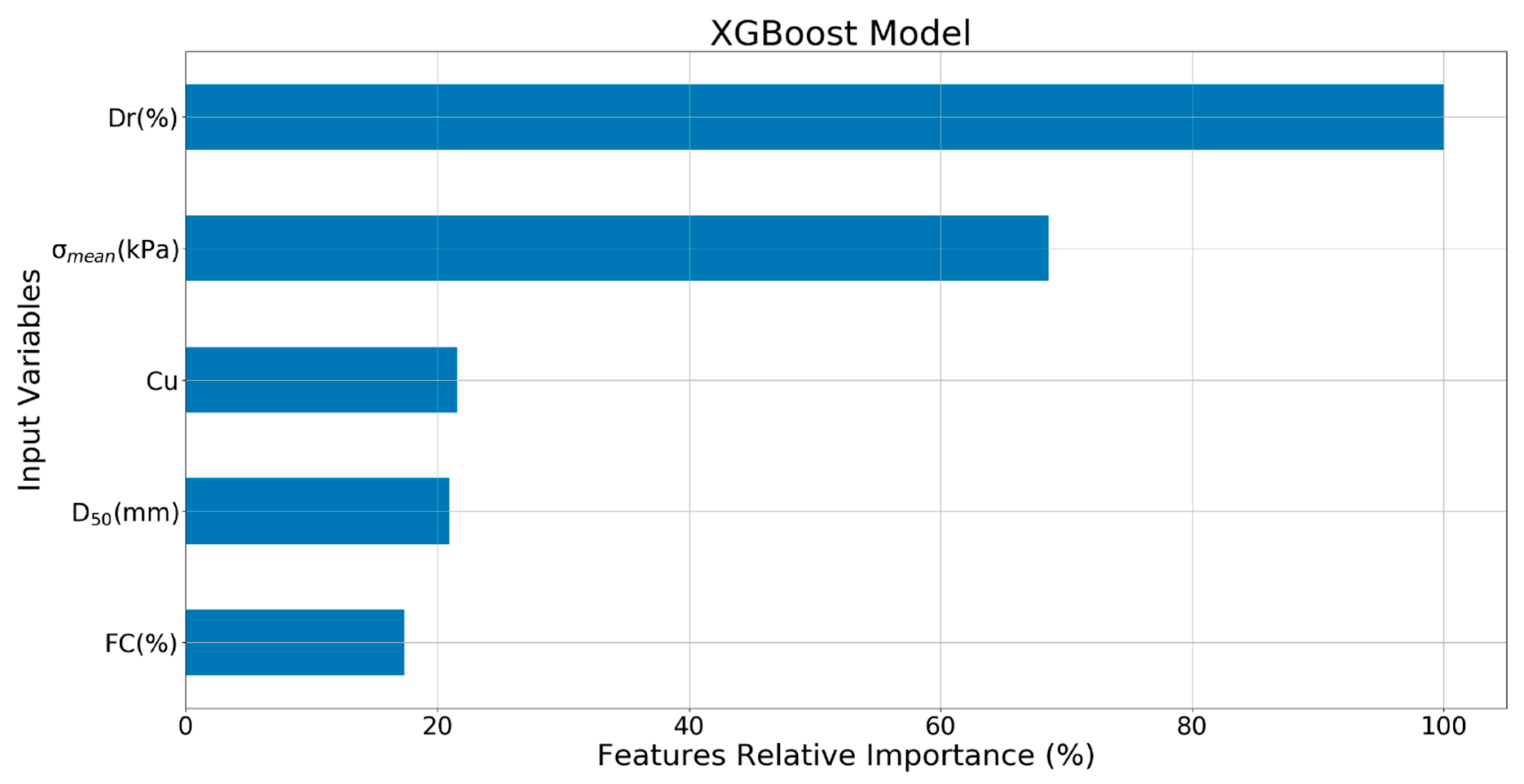
The relative importance of the input variables for XGBoost model is shown in Figure 27. It can be seen that Dr (100%) was the most important input variable, followed by (68.5%). Cu, D50, and FC had the relative importance of 21.6%, 20.9%, and 17.4%. All were quite small compared to that of Dr.
3.6. MARS Modeling Result
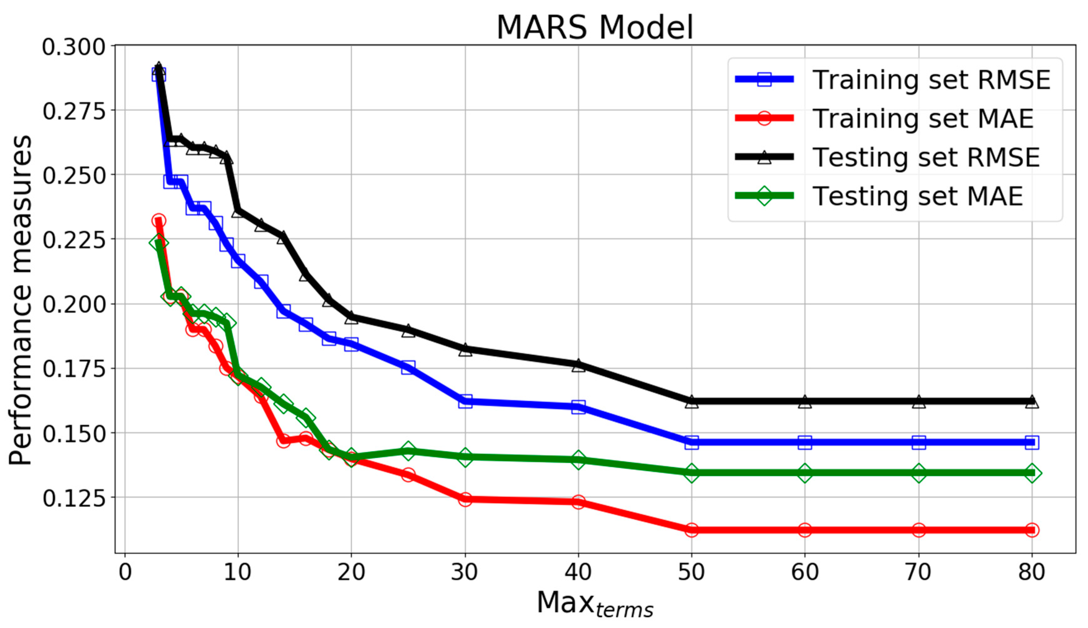
In the MARS model, the most important parameter is Maxterms, which controls the maximum number of terms generated by the forward pass. Figure 28 and Figure 29 give the RMSE, MAE, and R2 change curves of MARS model with parameter Maxterms. It can be seen that RMSE and MAE decreased and the R2 score increased with the increasing Maxterms until the value of 50, then the curves remained almost unchanged. The optimal Maxterms was chosen as 60.
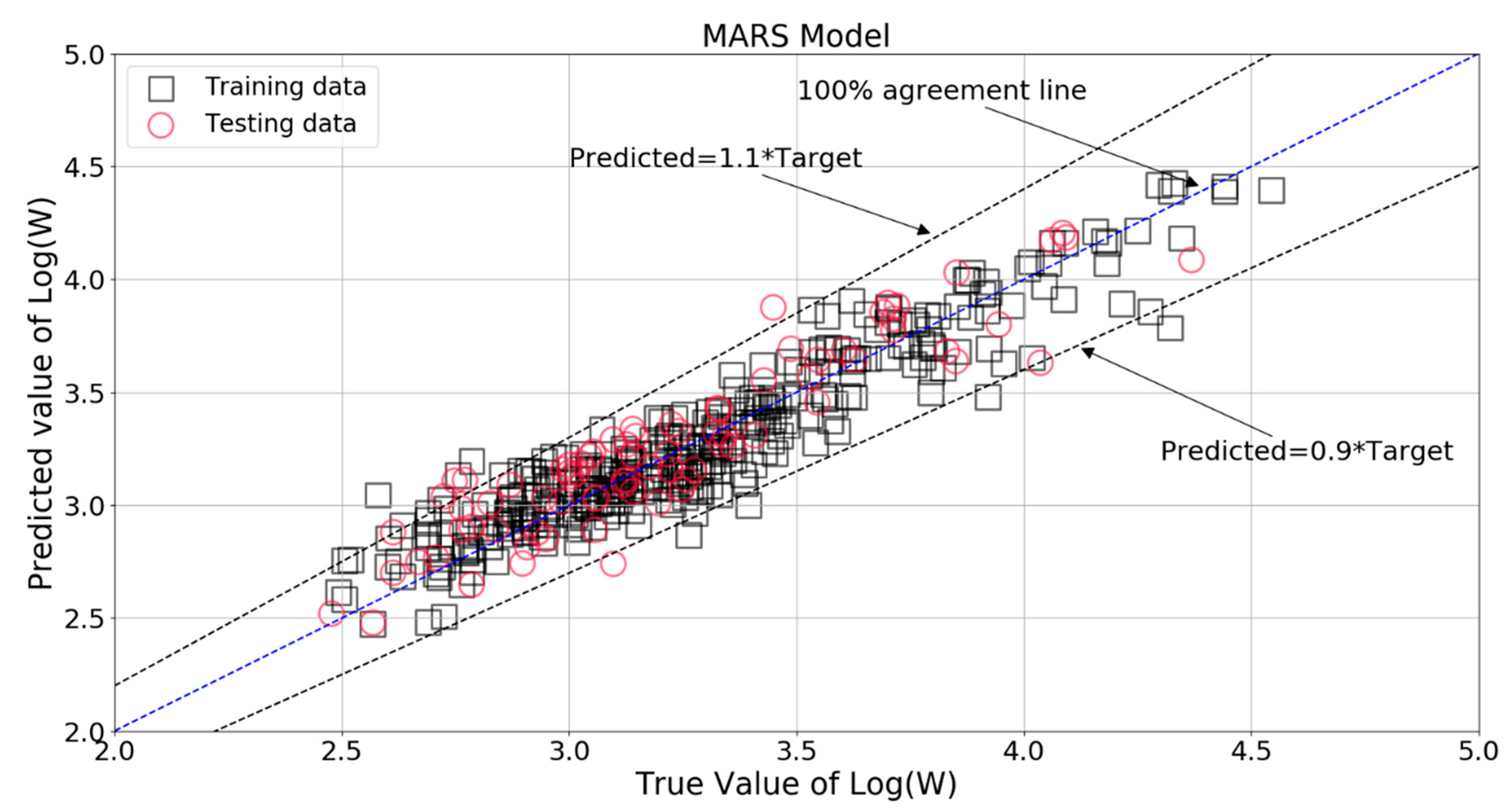
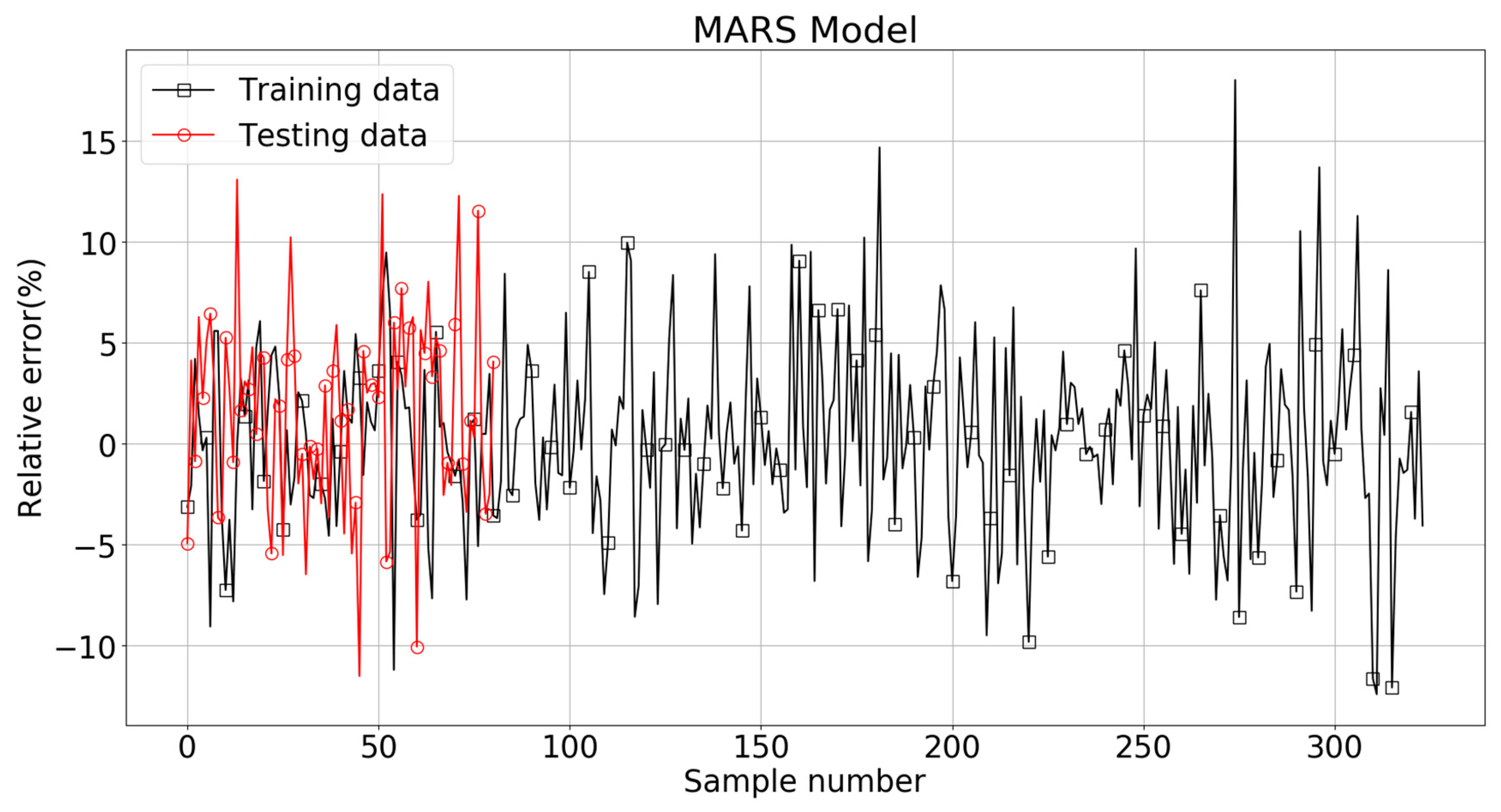
Figure 30 shows the comparison between true value and MARS model predicted value of Log(W). It can be seen that majority of the data points were within ± 10% of the target values. The relative errors for the training and testing patterns are plotted in Figure 31. Almost all of the MARS estimations of the training and testing set data fell within ± 10% of the target values. It should be noticed that the RMSE, MAE, and R2 scores were 0.148, 0.072, and 0.879 for the training set, with the corresponding scores of 0.165, 0.134, and 0.84 for the testing set. The results prove the satisfactory predictive capacities of MARS model.
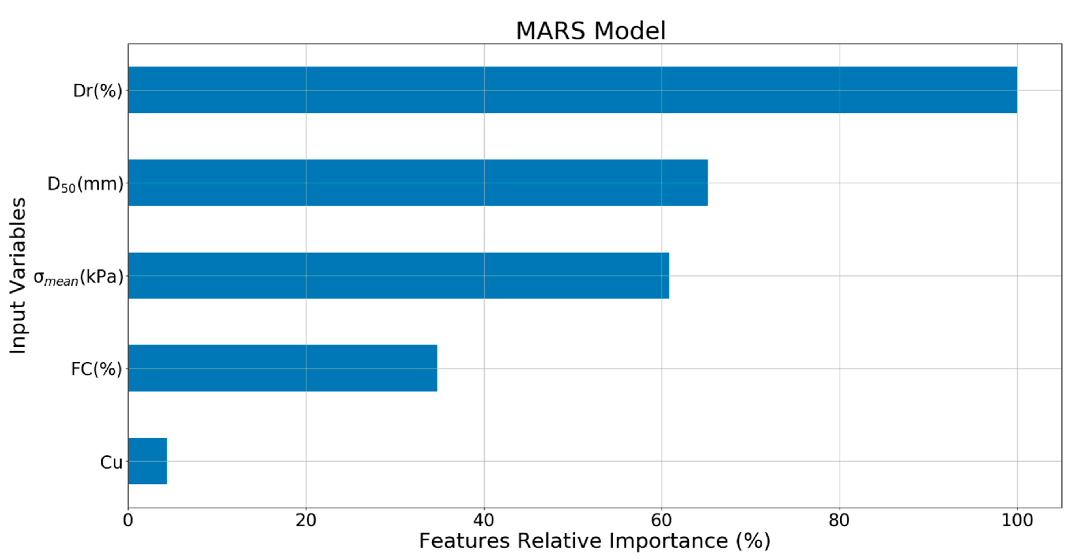
The relative importance of the input variables for MARS model are shown in Figure 32. It can be seen that Dr (100%) was the most important input variable, followed by D50 (65.2%), (60.9%), FC (34.8%), and Cu (4.34%).
Table 2 lists the basis functions (BFs) and their corresponding equation for the developed MARS model. It is observed from Table 2 that significant interactions have occurred between BFs (e.g., BF1 and BF2, BF2 and BF3, BF6 and BF7). The presence of interactions suggests that the built MARS model is not simply additive and that interactions play a significant role in building an accurate model for predictions. The equation of MARS model is given by Equation (26).
4. Comparison of the Results from Different Models
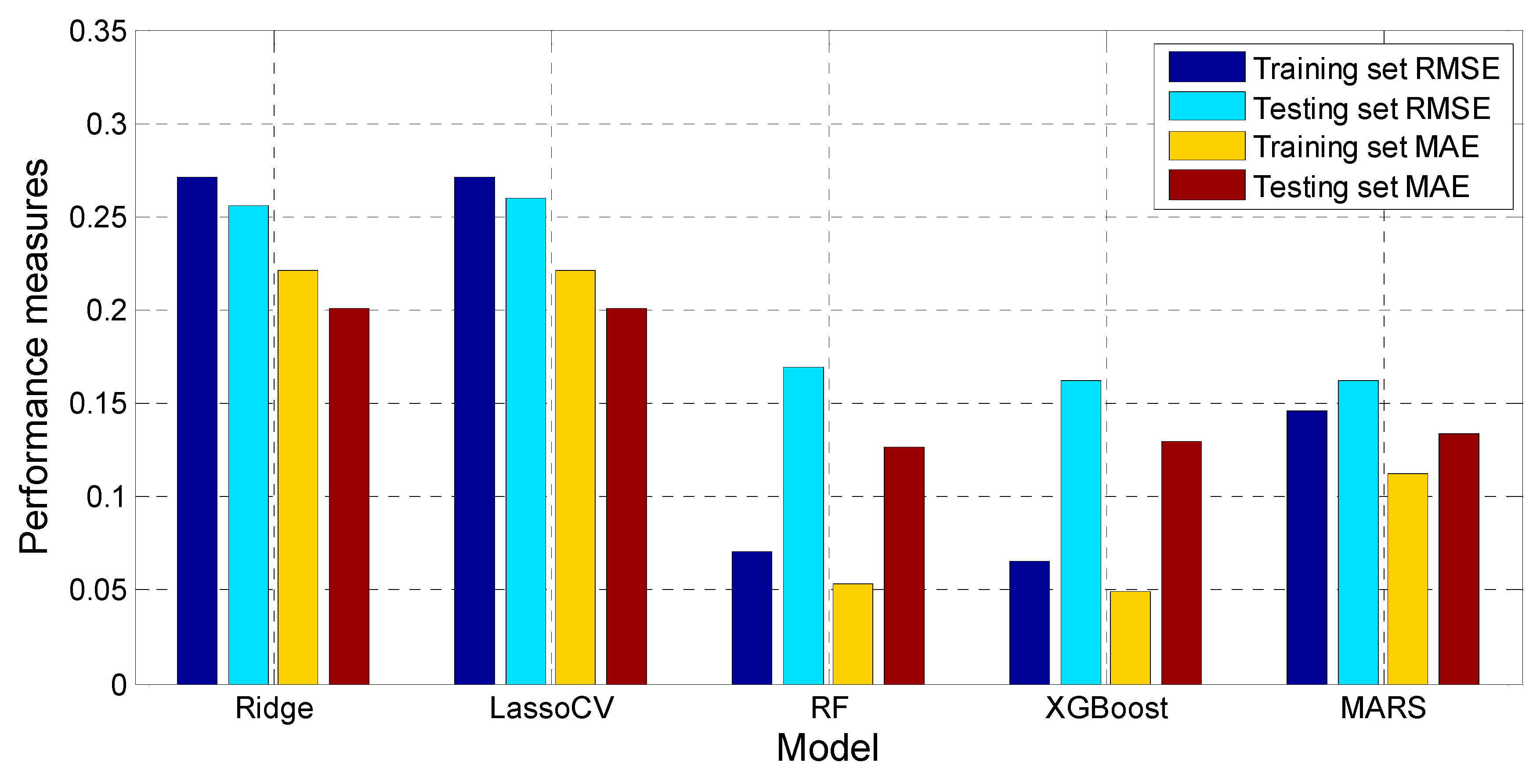
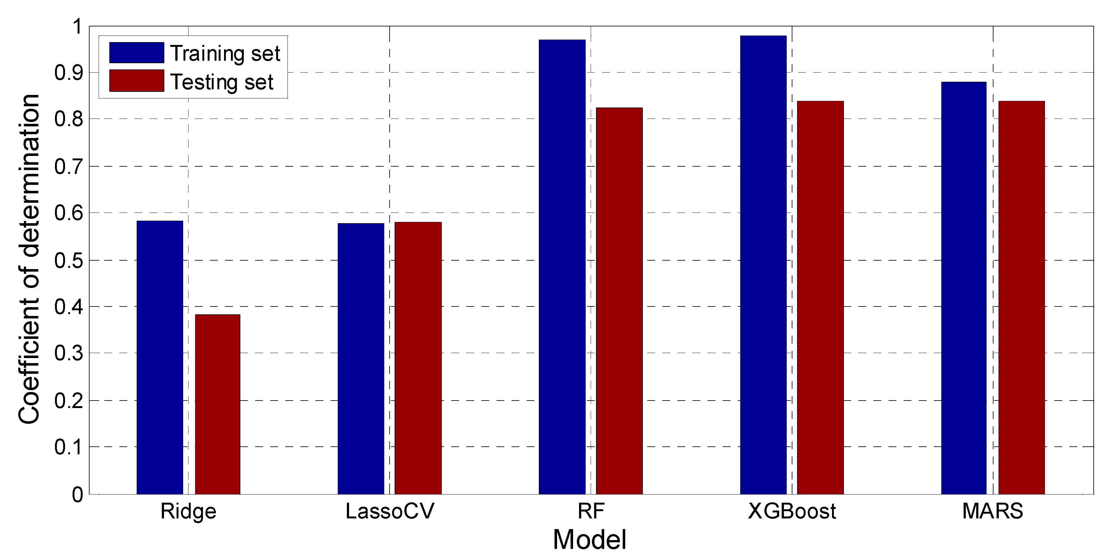
The performance indications of the Ridge, Lasso, RF, XGBoost, and MARS model for Soil Liquefaction Assessment using Capacity Energy Concept are listed in Figure 33 and Figure 34. It can be seen that the Ridge model performs worse among these five models. Its RMSE and MAE scores were 0.271 and 0.221 for the training set, with the corresponding scores of 0.258 and 0.201 for the testing set. The R2 scores were 0.582 and 0.382 for training set and testing set of Ridge model. The Ridge mode had the highest MRSE/MAE and lowest R2 score among these five models. This reflects the shortcoming of linear regression nature of Ridge model.
The Lasso & LassoCV model also did not perform well. The RMSE and MAE scores were 0.275 and 0.225 for the training set, and 0.255, 0.201 for the testing set. The R2 scores were 0.578 and 0.581 for training set and testing set, respectively. The RF, XGBoost, and MARS models achieved better results, whose RMSE and MAE values were smaller than 0.16 and 0.14, with the R2 scores were all above 0.8.
Overall, the R2 scores of RF and XGBoost models were higher than the MARS model, e.g., the R2 scores were 0.97 and 0.977 for training data for these two models, while the MARS was 0.879. This means that the RF and XGBoost model fit better than the MARS model in the training set. However, the R2 scores of the testing set for MARS model were 0.84, which is the same as the XGBoost model, and even higher than the RF model (0.825).
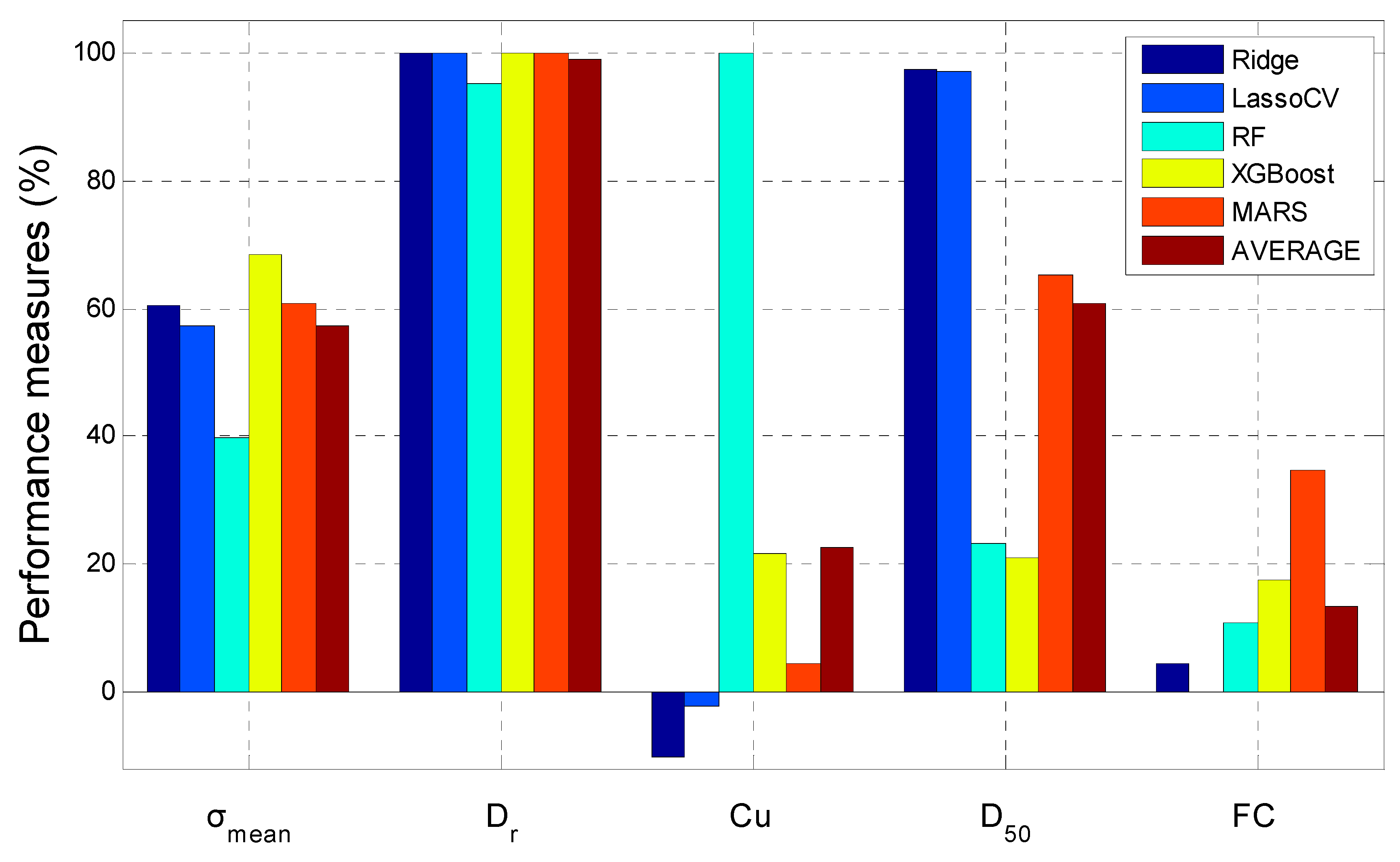
Figure 35 displays the relative importance of the input variables for the soil liquefaction assessment models developed by Ridge, Lasso & LassoCV, RF, XGBoost, and MARS. The results indicate that the capacity energy Log(W) was most sensitive to Dr, whose relative importance was almost 100% for all the five machine learning methods. The second important input variable should be either or , because their average relative importance were quite close and around 60%. But if we only focus on the RF, XGBoost, and MARS model whose performance measures were above 0.8, it can be found that the had the average relative importance of 56.4% while the had only 36.4%. The FC and Cu did not play a significant role, because their relative importance were all quite low for the five machine learning models. In addition, the LassoCV algorithm automatically removed the FC as input variable by giving it a zero regression coefficient. The relative importance of Cu were negative for Ridge and Lasso & LassoCV, and 21.6% and 4.34% for XGBoost model, which are all quite low.
It should be noticed that the performance of the MARS models were not only desirable, but the relative importance obtained by MARS model were also quite close to the average value of the five models. In addition, compared to the black box model of RF and XGBoost model, the MARS model had an advantage of the capacity to output explicit expressions.
5. Conclusions
In the present study, analyses have been carried out on a total of 405 previously published tests using machine learning algorithm, including Ridge, Lasso & LassoCV, Random Forest, XGBoost, and MARS approaches, to assess the capacity energy required to trigger liquefaction in sand and sandy soils. Major findings obtained in this research include:
(1) The performance measures for Ridge and Lasso & LassoCV models were all below 0.6, reflecting the shortage of linear regression methods in handling the complex data mapping in high-dimensional data sets.
(2) RF, XGBoost, and MARS models were capable of capturing the nonlinear relationships involving a multitude of variables with interaction among each other without making any specific assumption about the underlying functional relationship between the input variables and the response.
(3) Using the results of Ridge, Lasso & LassoCV, Random Forest, XGBoost, and MARS as cross-validation, it can be found that the capacity energy Log(W) was most sensitive to Dr, whose relative importance were almost 100% for all the five machine learning methods.
(4) The R2 scores of the testing set for MARS model was the same as the XGBoost model, and even higher than the RF model. The relative importance obtained by MARS model were quite close to the average value of the five models. In addition, compared to the black box model of RF and XGBoost model, the MARS model had an advantage of the capacity to output explicit expressions.
Author Contributions
Conceptualization, A.T.C.G. and W.Z.; methodology, W.Z.; software, C.W.; validation, Z.C., H.L. and C.W.; formal analysis, Z.C.; investigation, H.L.; resources, W.Z.; data curation, Z.C.; writing—original draft preparation, Z.C.; writing—review and editing, W.Z.; visualization, H.L.; supervision, W.Z.; project administration, W.Z.; funding acquisition, W.Z. All authors have read and agreed to the published version of the manuscript.
Funding
This research was funded by Natural Science Foundation (cstc2017jcyjAX0073), Chongqing.
Acknowledgments
The authors are grateful to the financial support from National Key R&D Program of China (Project No. 2019YFC1509600), Natural Science Foundation (cstc2017jcyjAX0073), Chongqing, Chongqing Construction Science and Technology Plan Project (No. 2019-0045) and Fundamental Research Funds for the Central Universities (Grant ID 2019CDJDTM0007).
Conflicts of Interest
The authors declare no conflict of interest.
References
- Lee, K.L.; Fitton, J.A. Factors affecting the cyclic loading strength of soil. In Vibration Effects of Earthquakes on Soils and Foundation; American Society for Testing and Materials (ASTM): West Conshohocken, PA, USA, 1969; pp. 71–95. [Google Scholar]
- Seed, H.B.; Idriss, I.M. Simplified procedure for evaluating soil liquefaction potential. Soil Mech. Found. Eng. 1971, 97, 1249–1273. [Google Scholar]
- Seed, H.B.; Idriss, I.M.; Makdisi, F.; Banerjee, N. Representation of Irregular Stress Time Histories by Equivalent Uniform Stress Series in Liquefaction Analyses; Report No. UCB/EERC-75/29; Earthquake Engineering Research Centre, University of California: Berkeley, CA, USA, 1975. [Google Scholar]
- Lee, Y.F.; Chi, Y.Y.; Lee, D.H.; Juang, C.H.; Wu, J.H. Simplified models for assessing annual liquefaction probability—A case study of the Yuanlin area, Taiwan. Eng. Geol. 2007, 90, 71–88. [Google Scholar] [CrossRef]
- Whitman, R.V. Resistance of soil to liquefaction and settlement. Soils Found. 1971, 11, 59–68. [Google Scholar] [CrossRef] [Green Version]
- Ishihara, K.; Yasuda, S. Sand liquefaction in hollow cylinder torsion under irregular excitation. Soils Found. 1975, 15, 45–59. [Google Scholar] [CrossRef] [Green Version]
- Juang, C.H.; Rosowsky, D.V.; Tang, W.H. Reliability-based method for assessing liquefaction potential of soils. J. Geotech. Geoenviron. Eng. 1999, 125, 684–689. [Google Scholar] [CrossRef]
- Juang, C.H.; Chen, C.J.; Jiang, T. Probabilistic framework for liquefaction potential by shear wave velocity. J. Geotech. Geoenviron. Eng. 2001, 127, 670–678. [Google Scholar] [CrossRef]
- Juang, C.H.; Ching, J.; Luo, Z.; Ku, C.S. New models for probability of liquefaction using standard penetration tests based on an updated database of case histories. Eng. Geol. 2012, 133, 85–93. [Google Scholar] [CrossRef]
- Moss, R.E.S.; Seed, R.B.; Kayen, R.E.; Stewart, J.P.; Der Kiureghian, A.; Cetin, K.O. CPT based probabilistic and deterministic assessment of in situ seismic soil liquefaction potential. J. Geotech. Geoenviron. Eng. 2006, 132, 1032–1051. [Google Scholar] [CrossRef] [Green Version]
- Boulanger, R.W.; Idriss, I.M. Probabilistic standard penetration test-based liquefaction-triggering procedure. J. Geotech. Geoenviron. Eng. 2012, 138, 1185–1195. [Google Scholar] [CrossRef]
- Green, R.A. Energy-based Evaluation and Remediation of Liquefiable Soils. Ph.D. Thesis, Virginia Polytechnic Institute and State University, Blacksburg, VA, USA, 2001. [Google Scholar]
- Baziar, M.H.; Jafarian, Y. Assessment of liquefaction triggering using strain energy concept and ANN model: Capacity energy. Soil Dyn. Earthq. Eng. 2007, 27, 1056–1072. [Google Scholar] [CrossRef]
- Dobry, R.; Ladd, R.S.; Yokel, F.Y.; Chung, R.M.; Powell, D. Prediction of Pore Water Pressure Build-up and Liquefaction of Sands During Earthquakes by the Cyclic Strain Method; National Institute of Standards and Technology (NIST): Gaithersburg, MD, USA, 1982.
- Seed, H.B. Closure to soil liquefaction and cyclic mobility evaluation for level ground during earthquakes. J. Geotech. Geoenviron. Eng. 1980, 106, 724. [Google Scholar]
- Davis, R.O.; Berrill, J.B. Energy dissipation and seismic liquefaction in sands. Earthq. Eng. Struct. Dyn. 1982, 10, 59–68. [Google Scholar]
- Nemat-Nasser, S.; Shokooh, A. A unified approach to densification and liquefaction of cohesionless sand in cyclic shearing. Can. Geotech. J. 1979, 16, 659–678. [Google Scholar] [CrossRef]
- Ostadan, F.; Deng, N.; Arango, I. Energy-based Method for Liquefaction Potential Evaluation, Phase I. Feasibility Study; National Institute of Standards and Technology (NIST): Gaithersburg, MD, USA, 1996.
- Baziar, M.H.; Jafarian, Y.; Shahnazari, H.; Movahed, V.; Tutunchian, M.A. Prediction of strain energy-based liquefaction resistance of sand–silt mixtures: An evolutionary approach. Comput. Geosci. 2011, 37, 1883–1893. [Google Scholar] [CrossRef]
- Figueroa, J.L.; Saada, A.S.; Liang, L.; Dahisaria, M.N. Evaluation of soil liquefaction by energy principles. J. Geotech. Geoenviron. Eng. 1994, 20, 1554–1569. [Google Scholar] [CrossRef]
- Liang, L. Development of an Energy Method for Evaluating the Liquefaction Potential of a Soil Deposit. Ph.D. Thesis, Department of Civil Engineering, Case Western Reserve University, Cleveland, OH, USA, 1995. [Google Scholar]
- Dief, H.M.; Figueroa, J.L. Liquefaction assessment by the energy method through centrifuge modeling. In NSF International Workshop on Earthquake Simulation in Geotechnical Engineering; Zeng, X.W., Ed.; CWRU: Cleveland, OH, USA, 2001. [Google Scholar]
- Chen, Y.R.; Hsieh, S.C.; Chen, J.W.; Shih, C.C. Energy-based probabilistic evaluation of soil liquefaction. Soil Dyn. Earthq. Eng. 2005, 25, 55–68. [Google Scholar] [CrossRef]
- Alavi, A.H.; Gandomi, A.H. Energy-based numerical models for assessment of soil liquefaction. Geosci. Front. 2012, 3, 541–555. [Google Scholar] [CrossRef] [Green Version]
- Cabalar, A.F.; Cevik, A.; Gokceoglu, C. Some applications of Adaptive Neuro-Fuzzy Inference System (ANFIS) in geotechnical engineering. Comput. Geotech. 2012, 40, 14–33. [Google Scholar] [CrossRef]
- Goh, A.T.C.; Zhang, W.; Zhang, Y.; Xiao, Y.; Xiang, Y. Determination of EPB tunnel-related maximum surface settlement: A Multivariate adaptive regression splines approach. Bull. Eng. Geol. Environ. 2018, 77, 489–500. [Google Scholar] [CrossRef]
- Zhang, W.G.; Goh, A.T.C. Multivariate adaptive regression splines for analysis of geotechnical engineering systems. Comput. Geotech. 2013, 48, 82–95. [Google Scholar] [CrossRef]
- Zhang, W.G.; Goh, A.T.C.; Xuan, F. A simple prediction model for wall deflection caused by braced excavation in clays. Comput. Geotech. 2015, 63, 67–72. [Google Scholar] [CrossRef]
- Zhang, W.G.; Goh, A.T.C.; Zhang, Y.M.; Chen, Y.M.; Xiao, Y. Assessment of soil liquefaction based on capacity energy concept and multivariate adaptive regression splines. Eng. Geol. 2015, 188, 29–37. [Google Scholar] [CrossRef]
- Zhang, W.G.; Goh, A.T.C.; Zhang, Y.M. Multivariate adaptive regression splines application for multivariate geotechnical problems with big data. Geotech. Geol. Eng. 2016, 34, 193–204. [Google Scholar] [CrossRef]
- Zhang, W.G.; Goh, A.T.C. Evaluating seismic liquefaction potential using multivariate adaptive regression splines and logistic regression. Geomech. Eng. 2016, 10, 269–284. [Google Scholar] [CrossRef]
- Zhang, W.G.; Goh, A.T.C. Multivariate adaptive regression splines and neural network models for prediction of pile drivability. Geosci. Front. 2016, 7, 45–52. [Google Scholar] [CrossRef] [Green Version]
- Zhang, W.G.; Zhang, R.H.; Goh, A.T.C. Multivaraite adaptive regression splines approach to estimate lateral wall deflection profiles caused by braced excavations in clays. Geotech. Geol. Eng. 2017. [Google Scholar] [CrossRef]
- Zhang, W.G.; Zhang, Y.M.; Goh, A.T.C. Multivariate adaptive regression splines for inverse analysis of soil and wall properties in braced excavation. Tunnel. Undergr. Space Technol. 2017, 64, 24–33. [Google Scholar] [CrossRef]
- Zhang, W.G.; Hou, Z.J.; Goh, A.T.C.; Zhang, R.H. Estimation of strut forces for braced excavation in granular soils from numerical analysis and case histories. Comput. Geotech. 2018, 106, 286–295. [Google Scholar] [CrossRef]
- Zhang, R.H.; Zhang, W.G.; Goh, A.T.C. Numerical investigation of pile responses caused by adjacent braced excavation in soft clays. Int. J. Geotech. Eng. 2018. [Google Scholar] [CrossRef]
- Zhang, W.G.; Wang, W.; Zhou, D.; Goh, A.T.C.; Zhang, R. Influence of groundwater drawdown on excavation responses – a case history in Bukit Timah granitic residual soils. J. Rock Mech. Geotech. Eng. 2018. [Google Scholar] [CrossRef]
- Zhang, W.G.; Goh, A.T.C.; Goh, K.H.; Chew, O.Y.S.; Zhou, D.; Zhang, R. Performance of braced excavation in residual soil with groundwater drawdown. Undergr. Space 2018, 3, 150–165. [Google Scholar] [CrossRef]
- Zhang, W.; Zhang, R.; Wang, W.; Zhang, F.; Goh, A.T.C. A Multivariate Adaptive Regression Splines model for determining horizontal wall deflection envelope for braced excavations in clays. Tunnel. Undergr. Space Technol. 2019, 84, 461–471. [Google Scholar] [CrossRef]
- Zhang, W.; Wu, C.; Zhong, H.; Li, Y.; Wang, L. Prediction of undrained shear strength using extreme gradient boosting and random forest based on Bayesian optimization. Geosci. Front. 2020. [Google Scholar] [CrossRef]
- Zhang, W.; Li, Y.; Wu, C.; Li, H.; Goh, A.T.C.; Lin, H. Prediction of lining response for twin tunnels construction in anisotropic clays using machine learning techniques. Undergr. Space 2020. [Google Scholar] [CrossRef]
- Hoerl, A.E.; Kennard, R.W. Ridge regression: Biased estimation for nonorthogonal problems. Technometrics 1970, 12, 55–67. [Google Scholar] [CrossRef]
- Buonaccorsi, J.P. A modified estimating equation approach to correcting for measurement error in regression. Biometrika 1996, 83, 433–440. [Google Scholar] [CrossRef]
- Stephen, G.W.; Christopher, J.P. Generalized ridge regression and a generalization of the Cp statistic. J. Appl. Stat. 2001, 28, 911–922. [Google Scholar]
- Hoerl, A.E.; Kennard, R.W.; Baldwin, K.F. Ridge regression: Some simulations. Commun. Stat. 1975, 4, 105–123. [Google Scholar] [CrossRef]
- Tibshirani, R. The lasso method for variable selection in the Cox model. Statist. Med. 1997, 16, 385–395. [Google Scholar] [CrossRef] [Green Version]
- Osborne, M.R.; Presnell, B.; Turlach, B.A. A new approach to variable selection in least squares problems. IMA J. Numer. Anal. 2000, 20, 389–403. [Google Scholar] [CrossRef] [Green Version]
- Donoho, D.; Johnstone, I.; Kerkyacharian, G.; Picard, D. Wavelet Shrinkage: Asymptopia? (with discussion). J. R. Stat. Soc. Ser. B 1995, 57, 301–337. [Google Scholar]
- Donoho, D.; Huo, X. Uncertainty Principles and Ideal Atomic Decompositions. IEEE Trans. Inf. Theory 2002, 47, 2845–2863. [Google Scholar] [CrossRef] [Green Version]
- Donoho, D.; Elad, M. Optimally Sparse Representation in General (Nonorthogonal) Dictionaries via L1-Norm Minimizations. Proc. Natl. Acad. Sci. USA 2003, 100, 2197–2202. [Google Scholar] [CrossRef] [PubMed] [Green Version]
- Donoho, D. For Most Large Underdetermined Systems of Equations, the Minimal L1-Norm Solution is the Sparsest Solution. Commun. Pure Appl. Math. 2006, 59, 907–934. [Google Scholar] [CrossRef]
- Meinshausen, N.; Bühlmann, P. Variable Selection and High-Dimensional Graphs With the Lasso. Ann. Stat. 2006, 34, 1436–1462. [Google Scholar] [CrossRef] [Green Version]
- Breiman, L. Random forests. Mach. Learn. 2001, 45, 5–32. [Google Scholar] [CrossRef] [Green Version]
- Kontschieder, P.; Bulò, S.R.; Bischof, H.; Pelillo, M. Structured class-labels in random forests for semantic image labelling. In 2011 International Conference on Computer Vision; IEEE: Piscataway, NJ, USA, 2011; pp. 2190–2197. [Google Scholar]
- Breiman, L.; Friedman, J.; Stone, C.J.; Olshen, R.A. Classification and Regression Trees; CRC Press: Boca Raton, FL, USA, 1984. [Google Scholar]
- Criminisi, A.; Shotton, J.; Konukoglu, E. Decision forests: A unified framework for classification, regression, density estimation, manifold learning and semi-supervised learning. Found. Trends® Comput. Graph. Vis. 2012, 7, 81–227. [Google Scholar] [CrossRef]
- Therneau, T.M.; Atkinson, E.J. An Introduction to Recursive Partitioning Using the RPART Routines; Mayo Clinic: Rochester, NY, USA, 1997. [Google Scholar]
- Chen, T.; Guestrin, C. Xgboost: A scalable tree boosting system. In Proceedings of the 22nd Acm Sigkdd International Conference on Knowledge Discovery and Data Mining, San Francisco, CA, USA, 13–17 August 2016; ACM: New York, NY, USA, 2016; pp. 785–794. [Google Scholar]
- Friedman, J.H. Multivariate adaptive regression splines. Ann. Stat. 1991, 19, 1–67. [Google Scholar] [CrossRef]
- Hastie, T.; Tibshirani, R.; Friedman, J. The Elements of Statistical Learning: Data Mining, Inference and Prediction, 2nd ed.; Springer: New York, NY, USA, 2009. [Google Scholar]
- Attoh-Okine, N.O.; Cooger, K.; Mensah, S. Multivariate adaptive regression spline (MARS) and hinged hyper planes (HHP) for doweled pavement performance modeling. Constr. Build. Mater. 2009, 23, 3020–3023. [Google Scholar] [CrossRef]
- Zarnani, S.; El-Emam, M.; Bathurst, R.J. Comparison, of numerical and analytical solutions for reinforced soil wall shaking table tests. Geomech. Eng. 2011, 3, 291–321. [Google Scholar] [CrossRef]
- Samui, P.; Karup, P. Multivariate adaptive regression spline and least square support vector machine for prediction of undrained shear strength of clay. Int. J. Appl. Metaheuristic Comput. 2011, 3, 33–42. [Google Scholar] [CrossRef]
- Lashkari, A. Prediction of the shaft resistance of non-displacement piles in sand. Int. J. Numer. Anal. Methods Geomech. 2012, 37, 904–931. [Google Scholar] [CrossRef]
- Khoshnevisan, S.; Juang, H.; Zhou, Y.G.; Gong, W. Probabilistic assessment of liquefaction-induced lateral spreads using CPT-Focusing on the 2010–2011 Canterbury earthquake sequence. Eng. Geol. 2015, 192, 113–128. [Google Scholar] [CrossRef]
- Kisi, O.; Shiri, J.; Tombul, M. Modeling rainfall-runoff process using soft computing techniques. Comput. Geosci. 2013, 51, 108–117. [Google Scholar] [CrossRef]
- Nagelkerke, N.J.D. A note on a general definition of the coefficient of determination. Biometrika 1991, 78, 691–692. [Google Scholar] [CrossRef]
Figure 1.
Typical stress–strain relationship during undrained cyclic triaxial test [18].
Figure 1.
Typical stress–strain relationship during undrained cyclic triaxial test [18].

Figure 2.
Spearman rank correlation coefficient for input variables.

Figure 3.
Schematic representation a RF classifier with N trees.

Figure 4.
Illustration of Random Forest regression construction.

Figure 5.
Schematic of XGBoost trees.

Figure 6.
Knots and linear splines for a simple MARS example.

Figure 7.
Root mean square error (RMSE) and mean absolute error (MAE) versus parameter for the Ridge model.
Figure 7.
Root mean square error (RMSE) and mean absolute error (MAE) versus parameter for the Ridge model.

Figure 8.
R2 change curve of the Ridge model with parameter .

Figure 9.
Comparison between the target and Ridge model predicted Log(W).

Figure 10.
Variation of the relative errors obtained from the Ridge model.

Figure 11.
Relative importance of the input variables for the developed Ridge model.

Figure 12.
RMSE and MAE versus parameter λ for the Lasso model.

Figure 13.
R2 change curve of the Lasso model with parameter λ.

Figure 14.
Comparison between the target and Lasso model predicted Log(W).

Figure 15.
Variation of the relative errors obtained from the Lasso model.

Figure 16.
Relative importance of the input variables for the developed LassoCV model.

Figure 17.
RMSE and MAE versus parameter nestimators for the RF model.

Figure 18.
R2 change curve of the RF model with parameter nestimators.

Figure 19.
R2 change curve of the Random Forest (RF) model with parameters min_samples_split and min_samples_leaf.
Figure 19.
R2 change curve of the Random Forest (RF) model with parameters min_samples_split and min_samples_leaf.

Figure 20.
Comparison between the target and RF model predicted Log(W).

Figure 21.
Variation of the relative errors obtained from the RF model.

Figure 22.
Importance of the input variables for the developed RF model.

Figure 23.
RMSE and MAE versus parameter estimators for the eXtreme Gradient Boost (XGBoost) model.

Figure 24.
R2 change curve of XGBoost model with parameter nestimators.

Figure 25.
Comparison between the target and XGBoost model predicted Log(W).

Figure 26.
Variation of the relative errors obtained from XGBoost model.

Figure 27.
Relative importance of the input variables for the developed XGBoost model.

Figure 28.
RMSE and MAE versus parameter Maxterms for MARS model.

Figure 29.
R2 change curve of MARS model with parameter Maxterms.

Figure 30.
Comparison between the target and MARS model predicted Log(W).

Figure 31.
Variation of the relative errors obtained from the MARS model.

Figure 32.
Relative importance of the input variables for the developed MARS model.

Figure 33.
Performance measures of the Ridge, Lasso, RF, XGBoost, and MARS model.

Figure 34.
R2 scores of the Ridge, Lasso, RF, XGBoost, and MARS model.

Figure 35.
Comparison of the relative importance of the input variables.


Table 1.
Statistics of parameters used for Multivariate Adaptive Regression Splines (MARS) model development.
Table 1.
Statistics of parameters used for Multivariate Adaptive Regression Splines (MARS) model development.
| Variables | Variable Description | Minimum | Maximum | Mean | Standard Deviation |
|---|---|---|---|---|---|
| Inputs | |||||
| (kPa) | Initial effective mean confining pressure | 40 | 400 | 103.2 | 50.8 |
| (%) | Initial relative density after consolidation | −44.5 | 105.1 | 51.6 | 29.8 |
| FC (%) | Percentage of fines content | 0 | 100 | 18.8 | 24.2 |
| Cu | Coefficient of uniformity | 1.52 | 28.1 | 4.14 | 6.09 |
| (mm) | Mean grain size | 0.03 | 0.46 | 0.21 | 0.12 |
| Outputs | |||||
| Logarithm of capacity energy | 2.48 | 4.54 | 3.27 | 0.42 |
Table 2.
Expressions of basis functions (BFs) for the MARS model.
| BF | Expression | BF | Expression |
|---|---|---|---|
| BF1 | D50 | BF11 | max(0, 56.9−Dr) × D50 × D50 |
| BF2 | max(0, −97.2) × D50 | BF12 | max(0, 67−Dr) × × max(0, 97.21−) |
| BF3 | max(0, −97.2) | BF13 | max(0, −82.74) |
| BF4 | Dr × D50 | BF14 | FC × max(0, Dr−68) × D50 |
| BF5 | FC × Dr × D50 | BF15 | max(0, 160−) × max(0, 90.18−Dr) |
| BF6 | D50 × D50 | BF16 | × max(0, 82.74−) |
| BF7 | FC × D50 × D50 | BF17 | × FC |
| BF8 | max(0, Dr−72.2) ×max(0, 90.18−Dr) | BF18 | max(0, Dr−75.1) × max(0, Dr−72.2) × max(0, 90.18−Dr) |
| BF9 | × max(0, 97.21−) | BF19 | max(0, 75.1−Dr) × max(0, Dr−72.2) × max(0, 90.18−Dr) |
| BF10 | max(0, Dr−56.9) × D50 × D50 | BF20 | FC × max(0, 72.2−Dr)×max(0, 90.18−Dr) |
© 2020 by the authors. Licensee MDPI, Basel, Switzerland. This article is an open access article distributed under the terms and conditions of the Creative Commons Attribution (CC BY) license (http://creativecommons.org/licenses/by/4.0/).
Share and Cite
MDPI and ACS Style
Chen, Z.; Li, H.; Goh, A.T.C.; Wu, C.; Zhang, W. Soil Liquefaction Assessment Using Soft Computing Approaches Based on Capacity Energy Concept. Geosciences 2020, 10, 330. https://0-doi-org.brum.beds.ac.uk/10.3390/geosciences10090330
AMA Style
Chen Z, Li H, Goh ATC, Wu C, Zhang W. Soil Liquefaction Assessment Using Soft Computing Approaches Based on Capacity Energy Concept. Geosciences. 2020; 10(9):330. https://0-doi-org.brum.beds.ac.uk/10.3390/geosciences10090330
Chicago/Turabian StyleChen, Zhixiong, Hongrui Li, Anthony Teck Chee Goh, Chongzhi Wu, and Wengang Zhang. 2020. "Soil Liquefaction Assessment Using Soft Computing Approaches Based on Capacity Energy Concept" Geosciences 10, no. 9: 330. https://0-doi-org.brum.beds.ac.uk/10.3390/geosciences10090330
Note that from the first issue of 2016, this journal uses article numbers instead of page numbers. See further details here.