An Empirical Model to Account for Spectral Amplification of Pulse-Like Ground Motion Records

Abstract

Near-source effects can amplify seismic ground motion, causing large demand to structures and thus their identification and characterization is fundamental for engineering applications. Among the most relevant features, forward-directivity effects may generate near-fault records characterized by a large velocity pulse and unusual response spectral shape amplified in a narrow frequency-band. In this paper, we explore the main statistical features of acceleration and displacement response spectra of a suite of 230 pulse-like signals (impulsive waveforms) contained in the NESS1 (NEar Source Strong-motion) flat-file. These collected pulse-like signals are analyzed in terms of pulse period and pulse azimuthal orientation. We highlight the most relevant differences of the pulse-like spectra compared to the ordinary (i.e., no-pulse) ones, and quantify the contribution of the pulse through a corrective factor of the spectral ordinates. Results show that the proposed empirical factors are able to capture the amplification effect induced by near-fault directivity, and thus they could be usefully included in the framework of probabilistic seismic hazard analysis to adjust ground-motion model (GMM) predictions.

1. Introduction

Near-fault effects are able to cause large seismic demand to structures compared to ground motion in far-field and thus their identification and characterization is fundamental for proper assessment of shaking for several engineering applications and seismic hazard analyses. These effects are related to a particular class of near-fault records characterized by pulses in the velocity traces, which can provide considerable input energy to sites located in the direction of propagation of the rupture (i.e., forward-directivity), when the rupture velocity is close to the shear-wave velocity [1]. Near-fault pulse-like motions may also be caused by fling-step [1,2,3]. Nevertheless, the two phenomena (i.e., fling-step and forward-directivity) implicate distinct characteristics on the time-series: directivity is associated with idealized full-cycle velocity pulses, while the fling-step is related to half-cycle pulses [1]. Moreover, directivity pulses show acceleration response spectra with larger narrow-band amplitudes and unusual shape; fling-step determines an offset at the end of the displacement record due to permanent tectonic deformation at the site. The latter causes amplifications in long-period spectral ordinates, while showing negligible effects on the acceleration response [4].

In this paper, we focus on forward-directivity effects identified by selecting the full-cycle pulses in the velocity time series, with the aim of investigating the pulse-like ground motion on spectral demand. These effects have been widely studied by many authors from the phenomenological point of view [1,2,3,4,5,6]; however, they are not yet fully included in the context of Probabilistic Seismic Hazard Analyses (PSHA) and consequently, the current seismic design codes do not provide a proper representation of these effects. In this framework, several authors have proposed simplified empirical approaches to adjust the ground-motion model (GMM) prediction with narrow-band amplification factors dependent on the pulse period [7,8,9,10,11,12]. This approach is currently the most practical one, and is different from the prior studies that proposed GMMs explicitly including directivity effects in the functional form [13] or models adjusted through broadband scaling factors [5].

However, the majority of these literature studies are based on limited near-fault datasets, so there is a need to investigate more extensively the pulse-like ground motion properties to calibrate statistically robust models.

In this paper, we explore the main statistical features and amplification effects of the impulsive records identified within a large dataset of near-fault records, i.e., the Near-Source Strong Motion flat-file (NESS1; https://0-doi-org.brum.beds.ac.uk/10.13127/NESS.1.0 [14,15]) to assess their impact on response spectra and calibrating an empirical corrective factor.

We thus modelled the narrow-band directivity factor based on the within-event part of the model residuals (i.e., the logarithmic difference between the observations and the model predictions) computed on a reference GMM specifically calibrated on the no-pulse (ordinary) records of the same dataset.

2. Near-Source Dataset

The present study takes advantage of the availability of a large number of high-quality waveforms collected within the NESS1 flat-file and containing the related intensity measures, event and station metadata. All the records of pan-European events in NESS1 are also available in the web portals of ITACA (Italian ACcelerometric Archive: http://itaca.mi.ingv.it; [16]) and ESM (Engineering Strong Motion: https://esm-db.eu; [17]). The NESS1 flat-file consists of about 800 three-component waveforms relative to 700 accelerometric stations, caused by 74 events with moment magnitude larger than 5.5 recorded in the 1933–2016 period. The NESS1 ground-motion data were selected to have a maximum source-to-site distance within one fault length, defined through seismological scaling relations. The accelerometric records were manually and uniformly processed, by using the ESM tool [18] that entails the application of a second-order acausal time-domain Butterworth filter. Most of the digital waveforms, which constitute about 70% of the dataset, were filtered with high-pass frequencies ≤ 0.1 Hz, whereas analog data were, on average, filtered at frequencies around 0.2 Hz, due to their lower quality [15]. The application of this type of filtering scheme, as known, does not allow recovery of the information about permanent displacement present in the time-series. Although such static deformation may be significant for near-source records, its estimation entails the adoption of baseline correction procedures (without band-pass filters), the details of which are beyond the scope of this work.

On these bases, an extensive investigation was performed on the NESS1 data by Pacor et al. [15], allowing recognition of the typical near-source effects, including velocity pulses. In particular, about 30% of the records were found to exhibit pulse-like characteristics, possibly due to forward-rupture directivity.

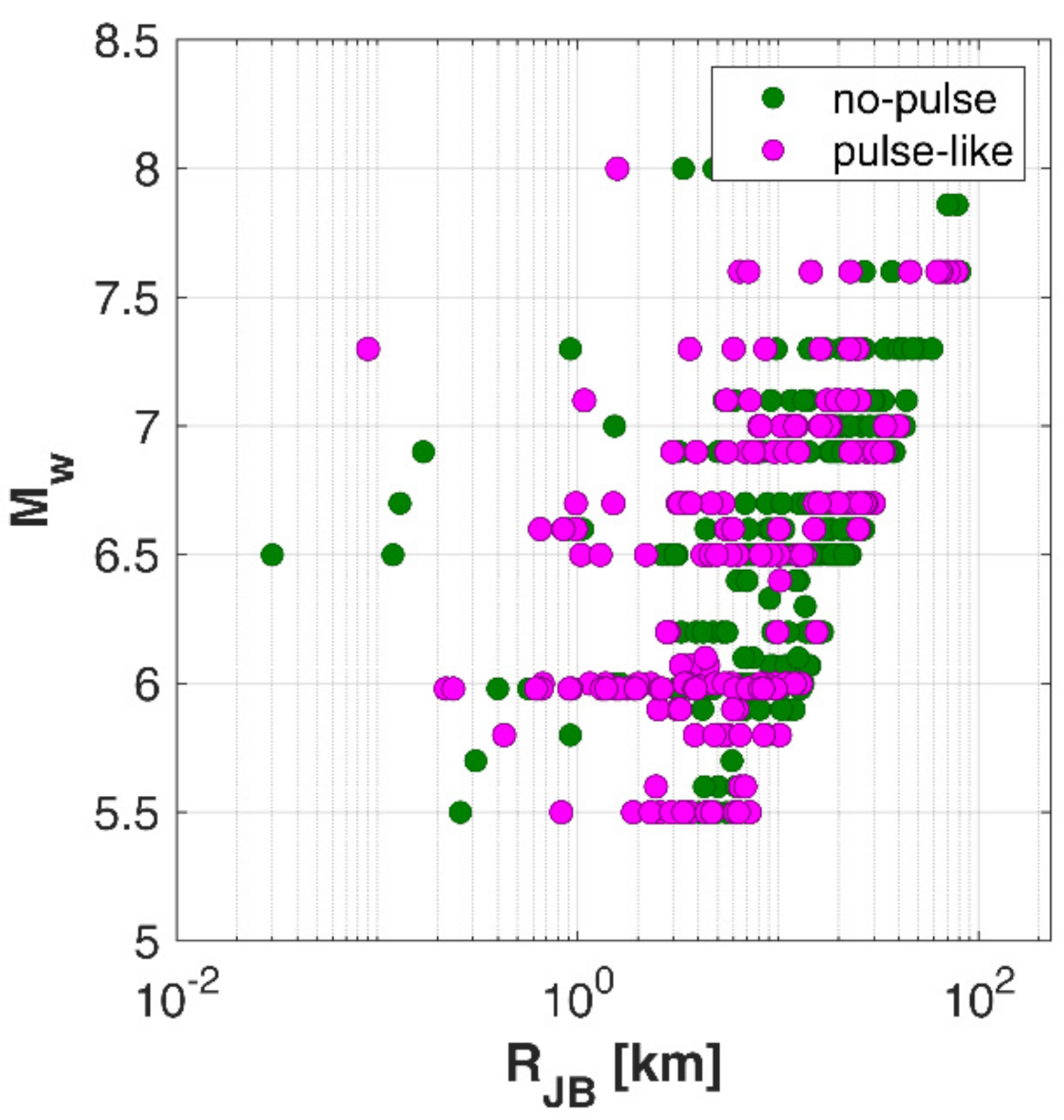
Figure 1 shows the moment magnitude M_w vs Joyner–Boore distance R_JB distribution of NESS1 data grouped into pulse-like (230 records from which we excluded 29 waveforms, having pulses potentially related to geotechnical effects) and no-pulse data (430 records). Both pulse-like and ordinary data are uniformly distributed over the magnitude-distance range of the dataset. The best sampled magnitude range is around M_w 6.0, due to the preponderance of highly sampled Italian data recorded during the seismic sequences of Northern Italy (2012) and Central Italy (2016), where relevant near-fault effects, also related to the presence of pulses, are observed.

3. Pulses Identification

For the investigation of pulse-like effects within the NESS1 dataset, the identification algorithm proposed by Baker [19] and Shashi and Baker [10] is herein applied. This procedure is largely adopted in the literature and is based on the use of a continuous wavelet transform of a single-component’s velocity time-history to extract the pulse from the horizontal orientations of each station’s records. In the algorithm implementation, a Pulse-Indicator (PI) score, as well as a lateness indicator (to exclude records with late-arriving pulse) are jointly assessed for each waveform without imposing any limits on peak ground velocity (PGV). The PI comprises a real number between 0 and 1: the larger the score, the more likely the record shows a pulse. Then, the criterion introduced by Shahi and Baker [10] is applied to each pair of horizontal components. Schematically, in a first step, ground motions with a PI > 0.85 according to [19] and that also exhibit PGV > 20 cm/s and/or trigger both criteria are flagged as pulse-like. In a second stage, all remaining ground motions that either trigger the Shahi and Baker [10] criterion alone or exhibit a PI > 0.50 are pooled together. These motions are then subjected to visual inspection of their velocity traces in the relevant orientations as well as of the azimuthal variation of their PI score. The pulse-like flag is also attributed to some of the ground motions in the second pool based on expert judgment and this represents an additional criterion to the original method.

The above procedure was systematically applied to all waveforms in the NESS1 flat-file, leading to a subset of 230 records identified and tagged as impulsive [15] along with the corresponding pulse period T_p (i.e., the pseudo-period of the wavelet extracted from the velocity signal) and pulse azimuthal orientation α_pulse.

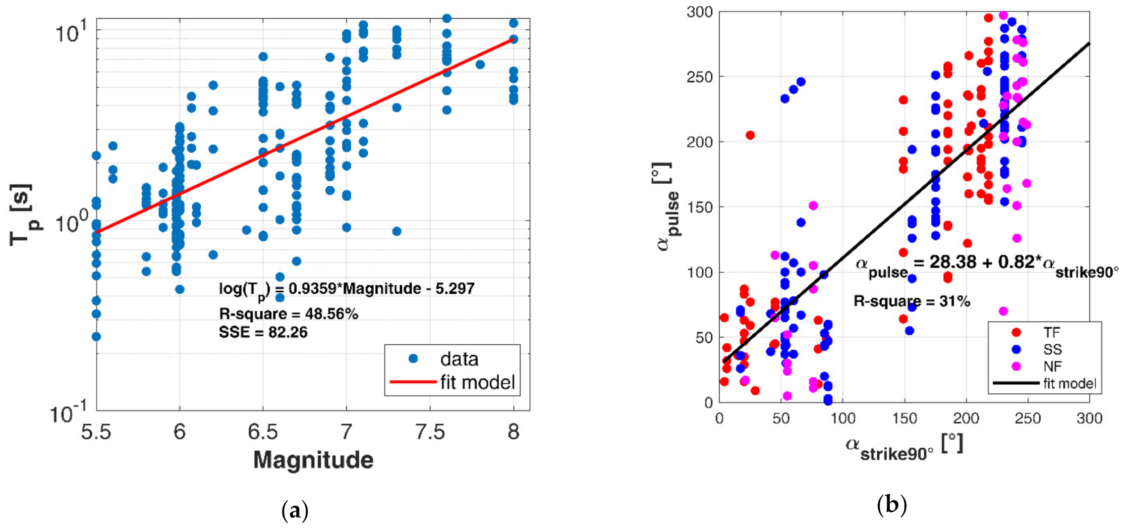
A scatter plot of the extracted pulse periods T_p versus magnitude of the causal events in NESS1 is reported in Figure 2a along with the corresponding least-squares linear regression model. As expected, we find that the logarithm of the mean of the pulse periods linearly depends on the event magnitude (M), according to the following empirical relationship:

$${\mu }_{\mathrm{lnTp}} = 0.9359\times \mathrm{M} – 5.297$$

(1)

This result is consistent with the fact that the period T_p is related to the rise time (i.e., duration of the slip at a single point on the fault) and the fault dimensions, tending to increase with magnitude; e.g., [5,6]. With reference to the pulse orientation (α_pulse), we observe that it correlates with the normal direction (90°) to the strike of the fault (α_strike90°) over all possible orientations of the strike angle, meaning that the pulses occur mainly on the fault normal (FN) direction, with no relevant differences for both Strike-Slip (SS) and dip-slip faults, that are Normal-Faulting (NF) and Thrust-Faulting (TF)—Figure 2b. On these data, we found the following relationship:

$${\mathsf{\alpha }}_{\mathrm{pulse}}=0.82\times {\mathsf{\alpha }}_{\mathrm{strike}90°}+23.38$$

(2)

4. Effect of Pulses on Elastic Spectral Response

As the main goal of the present study is to investigate the effect of the impulsive records on the response spectral shape, the NESS1 dataset is analyzed separately for pulse-like and ordinary waveforms to capture the most relevant differences in terms of spectral amplitudes and shapes.

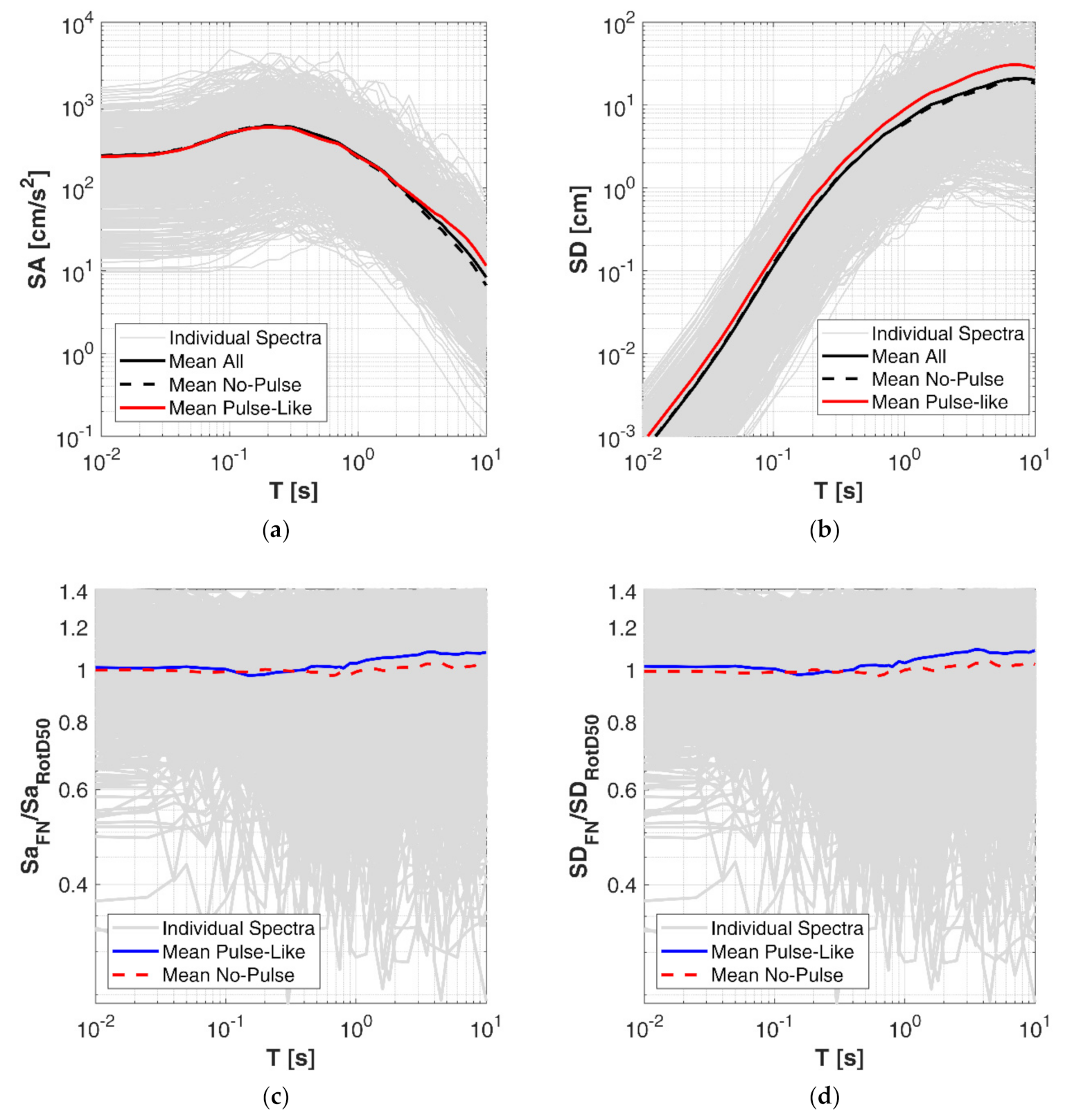
In Figure 3, we compare the pulse-like and no-pulse average elastic response spectra of 5%-damped acceleration SA (a) and displacement SD (b), with the aim of recognizing the overall effect of pulses on spectral shapes. It can be noted that SA response spectra are affected by pulse-like data at longer periods (T), mainly at T larger than 2 s, whereas on SD the amplification effect of the spectral ordinates is distributed over the whole period range from 0.01 s to 10 s. In this regard, we point out that, although the application of a high-pass filtering to the waveforms instead of a baseline correction procedure may affect the displacement response, it was found by D’Amico et al. [4] that the results obtained from the two schemes start to diverge only at very long periods (T > 5 s), causing underestimates of the spectral ordinates in case of filtering. Therefore, the above findings on the overall impact of impulsive records on displacement spectra remain still valid.

In the reported plots, the orientation independent component RotD50 [20] is considered; a comparison of the mean ratio between RotD50 and FN spectral ordinates is given in Figure 3 both for acceleration (c) and displacement (d) response spectra. The plots show that the mean ratio between the two components is practically near unity at all periods, with slightly larger differences at medium-longer periods (T > 0.5 s) where the ratio is, as expected, higher than 1, being the FN component more energetic. In the following analyses, we choose to show the FN components, being slightly larger than the RotD50 and more frequently used for calibration of directive GMMs. However, the main findings of this work are applicable to both types of components with small differences.

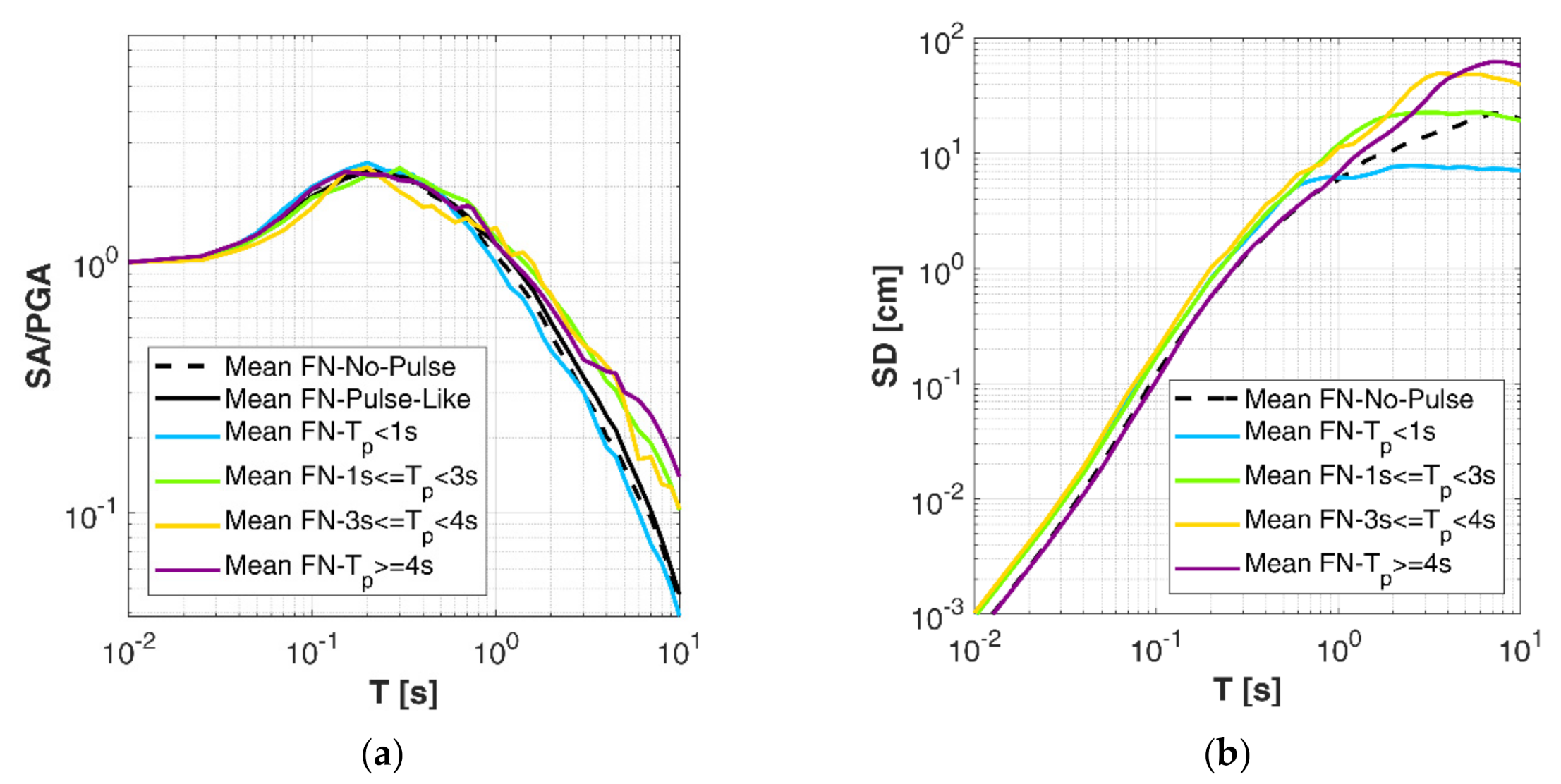
Previous studies on near-fault pulse-like motions showed the dependencies of: (i) the response spectra on the pulse period T_p [21,22] and (ii) the pulse period on earthquake magnitude [2,5,6,23]. To investigate this dependency on spectral ordinates, in Figure 4 we show a sensitivity analysis of normalized SA, i.e., divided by the PGA value (Figure 4a), and SD (Figure 4b) to different bins of the pulse period T_p, showing that spectral amplitudes become larger at longer periods as T_p increases, starting to deviate from the ordinary mean trend in correspondence of the average value of T_p in the bin. However, this effect is not visible for pulse periods shorter than 1 s. The SD (Figure 4b) are also markedly affected by T_p, showing broadband amplifications at period pulses larger than 1 s.

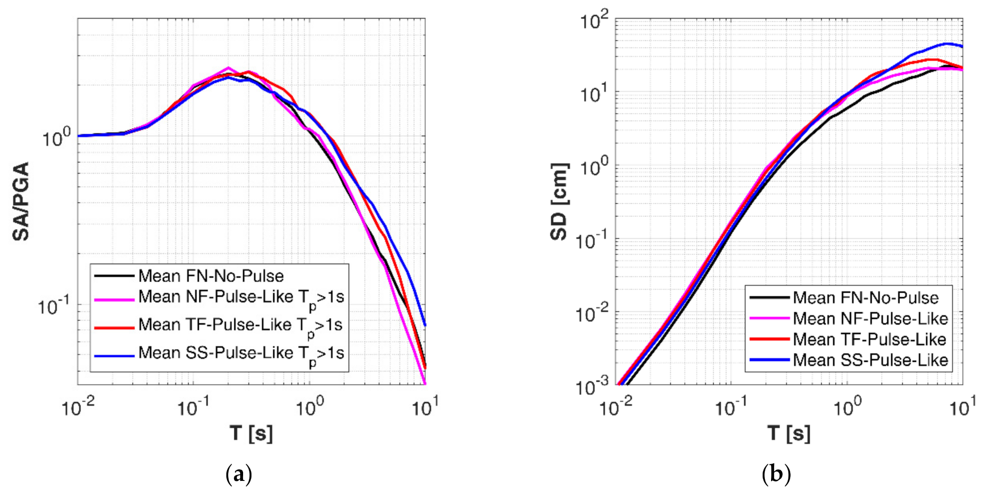
The effect of the style of faulting on pulse-like spectra is illustrated for the FN components on SA normalized to the PGA (a) and SD (b) in Figure 5.

This effect is investigated for ground motions related to NF, TF and SS earthquakes for some pulse period T_p bins. In these figures, the SA curves are plotted for pulse-like records with T_p larger than 1 s in order to enhance the shape differences of the normalized SA. It can be noted that SS earthquakes show systematically higher spectral ordinates, both for SA and SD than the other styles of faulting, particularly above a period of 2 s. This effect may achieve about 40% of amplification for SD with respect to ground motions from dip-slip earthquakes. Among the latter, the TF earthquakes provide larger ordinates compared to NF and no-pulse ground motion.

A possible physical explanation of this observation may be related to the correlation that lies between the rise time and the pulse period, which thus implies a correlation of T_p with the style of faulting. Indeed, according to [23,24], the rise time for dip-slip earthquakes is, on average, about half the rise time for SS earthquakes. As a result, the pulse period for an SS earthquake is expected to be longer than that for a dip-slip earthquake, thus producing more significant spectral amplifications at longer periods, as evidenced by our analysis.

5. Calibration of the Empirical Corrective Factor

5.1. Reference GMM of No-Pulse Records

The estimation of an empirical corrective factor accounting for pulse-like features is computed on the residuals of the subset of impulsive ground motions with respect to a reference GMM expressed in terms of SA(T). The latter is specifically calibrated for this aim on ground motions (both horizontal FN and RotD50 components) classified as no-pulse, in order to remove any bias from the mean. The 430 no-pulse records selected within NESS1 are within distances R_JB ≤ 50 km.

The functional form of the reference GMM is given in Equation (3) and includes the terms related to the source (F_M, Equation (4)), the distance attenuation, also describing the magnitude-dependent geometrical spreading (F_D, Equation (5)), the site (F_S, Equation (6)), the style of faulting (F_SOF, Equation (7)) and the error e (Equation (8)). The explanatory variables are the moment magnitude M_w, the source-to-site distance R, the shear wave velocity in the uppermost 30 m, V_S,30 and the styles of faulting SOF_j, which are dummy variables, introduced to specify SS (j = 1) and dip-slip, i.e., TF/NF (j = 2), fault types.

$${\log }_{10}\left(\mathrm{SA}\right)=\mathrm{a}+{\mathrm{F}}_{\mathrm{M}}+{\mathrm{F}}_{\mathrm{D}}+{\mathrm{F}}_S+{\mathrm{F}}_{\mathrm{SOF}}+ {\mathrm{r}}_{\mathrm{es}}$$

(3)

where:

F_M = b₁(M_w − M_h) for M ≤ M_h; F_M = b₂(M_w − M_h) for M > M_h,

(4)

F_D = [c₁(M_w − M_ref) + c₂] log₁₀(R),

(5)

F_S = k log₁₀(V₀/800) with V₀ = V_S,30 if V_S,30 < 1500 m/s or V₀ = 1500 m/s if V_S,30 ≥ 1500 m/s

(6)

F_SOF = δ_j SOF_j,

(7)

The hinge magnitude M_h, the reference magnitude M_ref and the pseudo-depth h are constants, which have been assumed as follows: M_h = 6.75; M_ref = 5.5 and h = 6 km according to the average values in the dataset.

The coefficients a, b₁, b₂, c₁, c₂, k and f_j (f₁ for SS, f₂ for TF and NF) are derived by a mixed-effect linear regression [25]. The predicted value by the model is a 10-base logarithm of the spectral acceleration SA (i.e., the peak ground acceleration, PGA and SA at 36 ordinates) at 5% damping in the period range 0.01–10 s. The model residuals r_es are partitioned into between-event (δB_e) and within-event (δWS_es) terms of error (Equation (8), thus the total variability σ associated to the GMM (Equation (9) is obtained through the combination of between-event (τ) and within-event (ϕ) standard deviations [26]:

r_es = δB_e + δWS_es (e = event; s = station)

(8)

σ = (τ² + ϕ²)^0.5

(9)

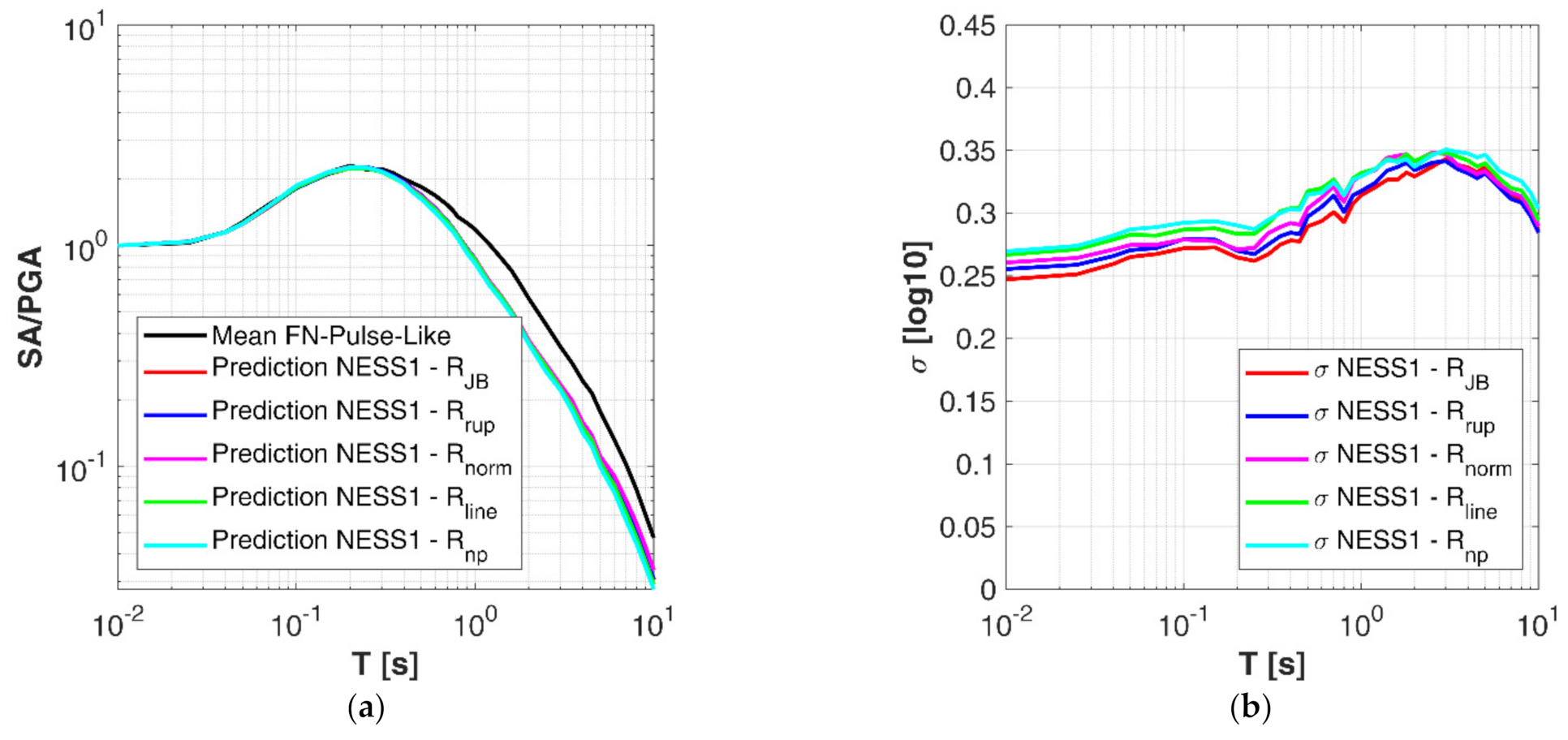
During the calibration stage, we derive different sets of coefficients for the different source-to-site metrics in order to select the most appropriate one for the GMM description: Joyner–Boore (R = R_JB); rupture (R = R_rup); rupture normalized to the fault length (R = R_norm); line (R = R_line) and nucleation-point (R = R_np) distances (for a detailed description on these distance metrics definitions, see [15]). We find that the model prediction (Figure 6a) and the total standard deviation σ (Figure 6b) computed as mean over all the ordinary records are almost insensitive to the adopted distance metric. In light of this, we decide to adopt the R_JB metric according to the majority of GMMs.

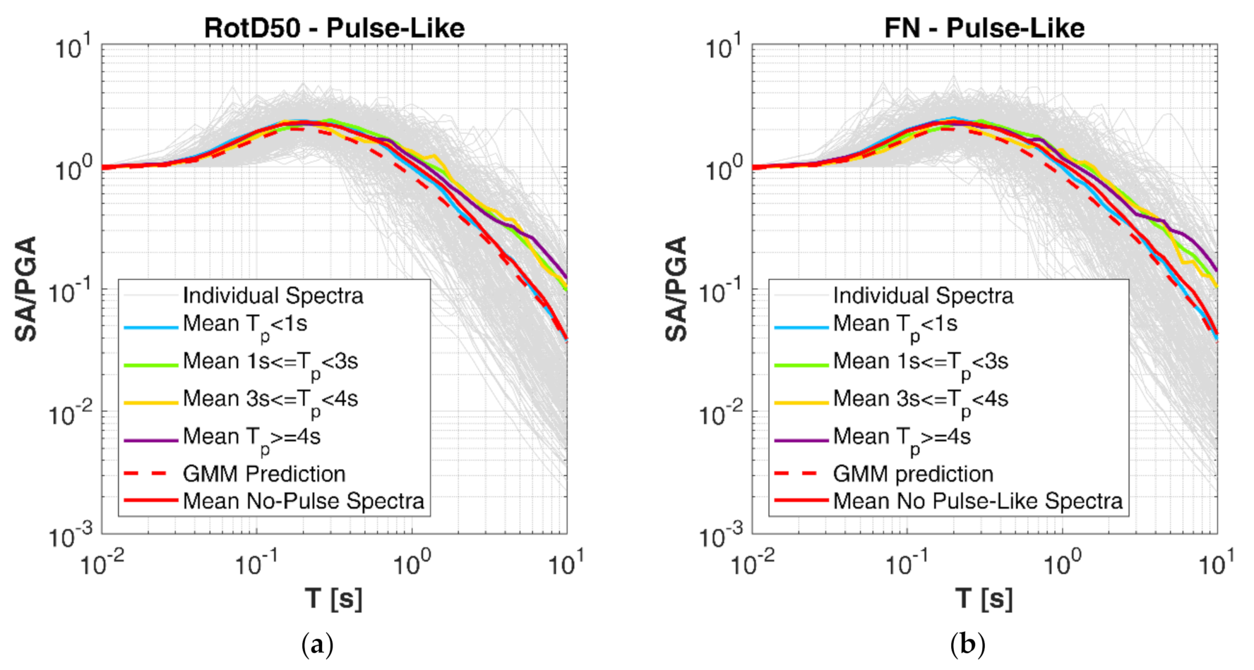
Figure 7 shows the GMM prediction (dashed line) compared to the mean of observed no-pulse and pulse-like data (solid lines), grouped by pulse periods. As expected, the GMM prediction is in good agreement with the mean of no-pulse motions, whereas a significant bias is noticeable for pulse-like records, especially at longer periods. No relevant differences between RotD50 (Figure 7a) and FN-based (Figure 7b) predictions can be observed.

5.2. Narrowband Amplification Factor

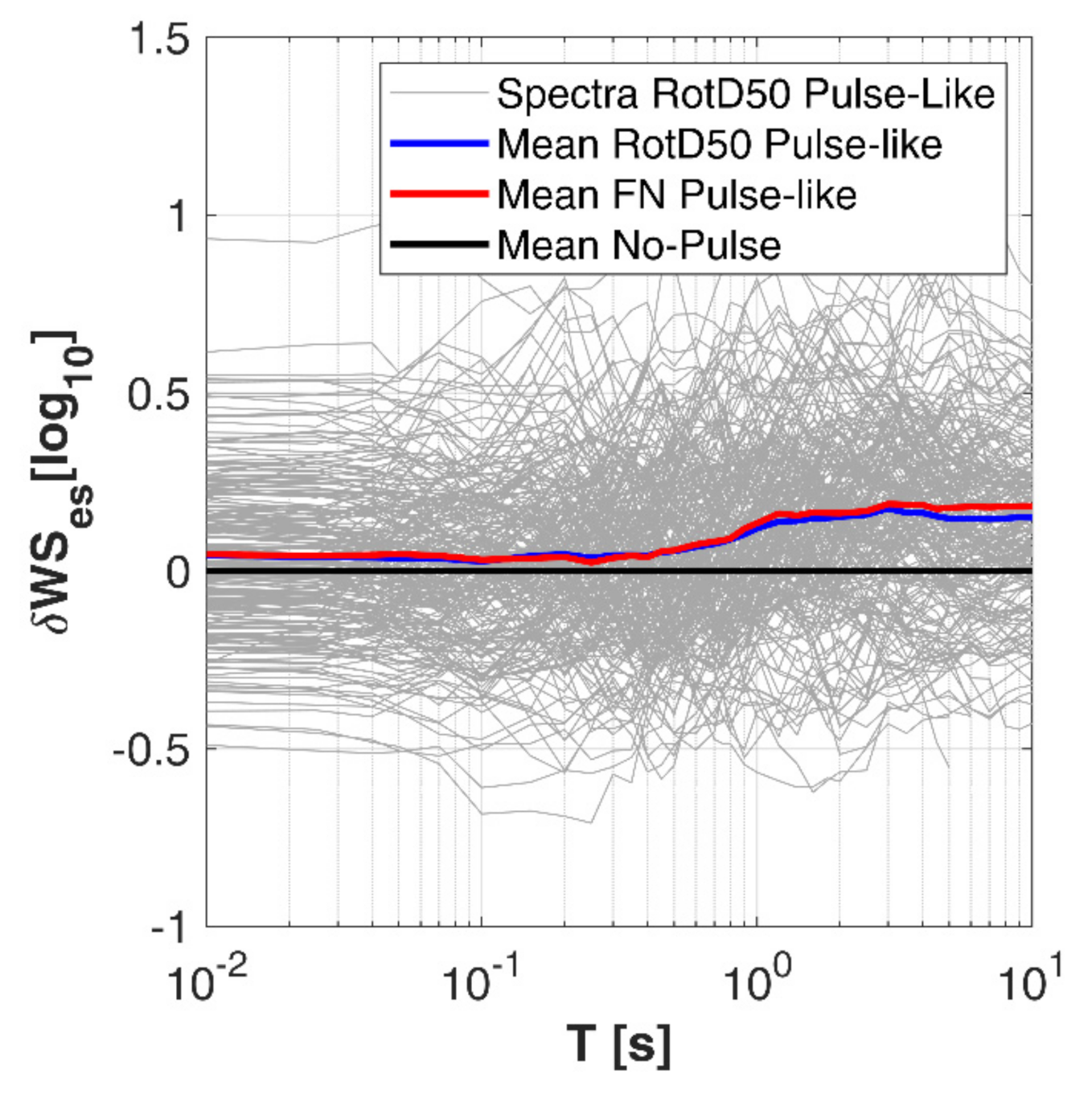
As discussed in the introduction, a practical approach to estimate spectral accelerations of impulsive records consists in using a GMM to predict ordinary motions (not impulsive) and then add an amplification factor around the pulse period to account for the contribution of the pulse [10]. To quantify this amplification effect on SA, we studied the within-event residuals of the observed acceleration spectral amplitudes with respect to that predicted by the GMM calibrated on no-pulse data. The residuals δWS_es versus period T are plotted in Figure 8.

The black thick line indicates that the mean of the residuals of no-pulse records is close to zero, suggesting that, on average, the calibrated GMM is good for SA prediction and thus can be used to model ordinary near-fault ground motions. The blue and red lines, instead, indicate the mean of the pulse-like residuals, respectively, in terms of RotD50 and FN components. These latter show systematic bias especially at longer periods (T > 0.6 s).

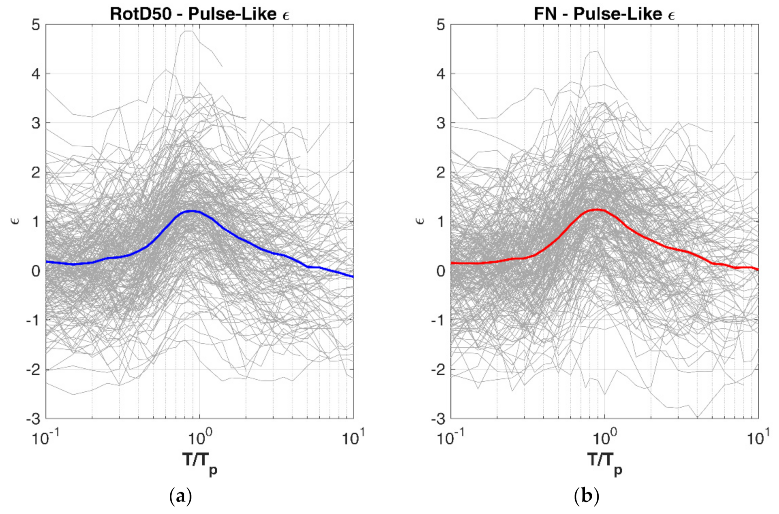
A more convenient form to check the amplification effect of impulsive data is obtained by plotting the within-event residuals normalized to the corresponding standard deviation (ε), as follows:

$$\mathsf{\epsilon }=\frac{{\mathsf{\delta }\mathrm{WS}}_{\mathrm{es}}\left(\mathrm{T}\right)}{\varphi \left(\mathrm{T}\right)}$$

(10)

This quantity is plotted versus the ratio T/T_p, as shown in Figure 9 for RotD50 (a) and FN (b) pulse-like waveforms. This approach to represent the residuals was also adopted by many authors [27,28,29,30,31].

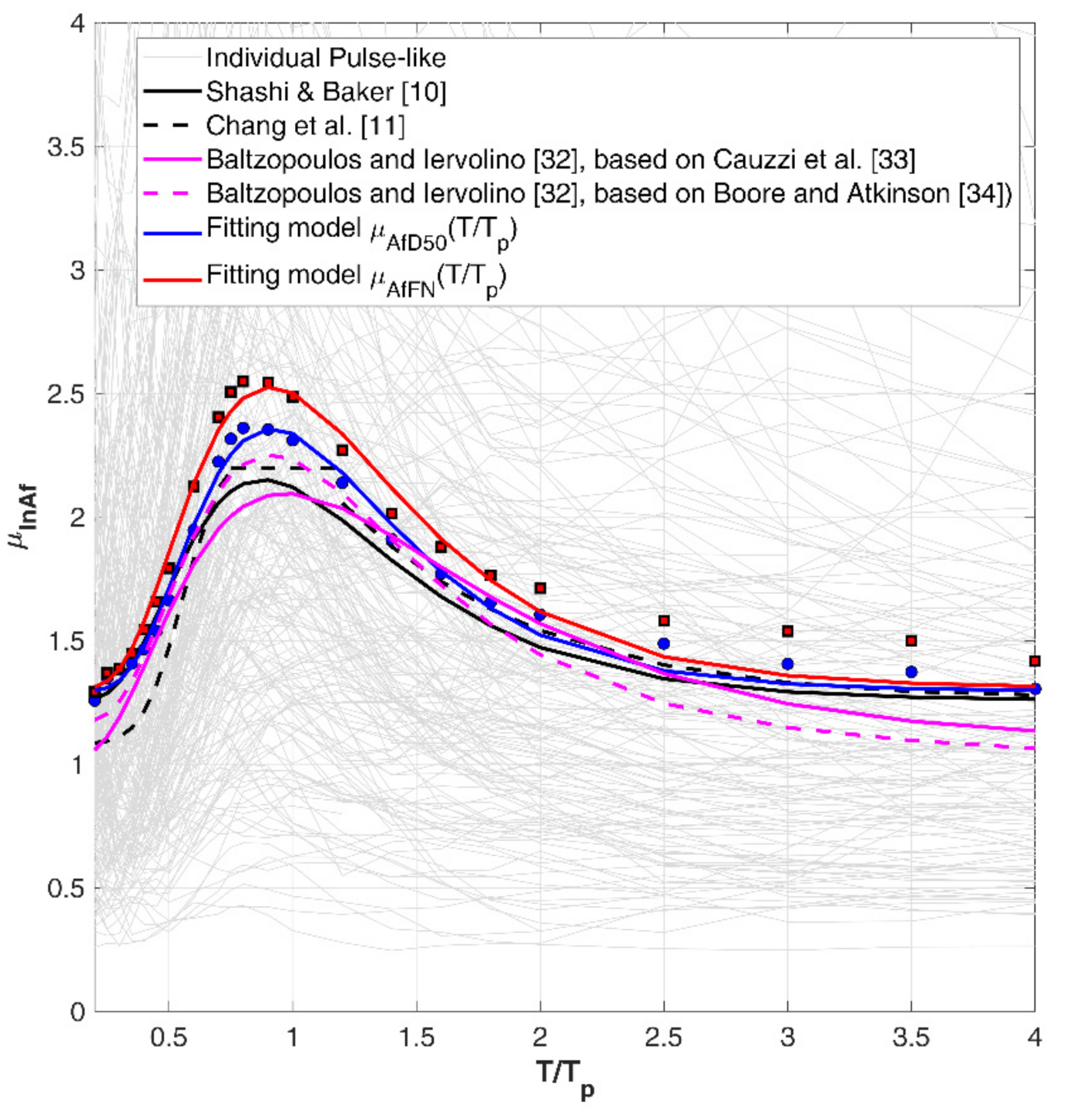
The introduction of the ratio T/T_p leads evident that the mean curve of the residuals has the typical bell-curve shape with a “bump” centered close to ratio T/T_p = 1. This shape of the mean amplification factor µ_Af is well approximated by Equations (11) and (12), respectively for RotD50 and FN components, calibrated through the curve fitting toolbox provided by Mathworks-Matlab^® environment:

$${\text{µ}}_{\mathrm{lnAf},\mathrm{D}50}=1.063\times \left[\exp {\left(\frac{-2.482{*\log }_{10}\left(\raisebox{1ex}{$\mathrm{T}$}\!\left/ \!\raisebox{-1ex}{${\mathrm{T}}_{\mathrm{P}}$}\right.\right)+0.0861}{0.98}\right)}^2\right]+1.294,$$

(11)

$${\text{µ}}_{\mathrm{lnAf},\mathrm{FN}}=1.22\times \left[\exp {\left(\frac{-{\log }_{10}\left(\raisebox{1ex}{$\mathrm{T}$}\!\left/ \!\raisebox{-1ex}{${\mathrm{T}}_{\mathrm{P}}$}\right.\right)-0.09347}{0.6734}\right)}^2\right]+1.305.$$

(12)

For Equation (11), the estimated goodness of fit in terms of RMSE is 0.055 (coefficient of determination R-squared 98.3%), whereas for Equation (12) the RMSE is equal to 0.077 (R-squared 97.4%).

Figure 10 shows that the calibrated amplification factors, in terms of the ratio between the spectral accelerations SA normalized to the GMM prediction, is consistent with those proposed by other authors [10,11,32,33,34]. The proposed models estimate systematically higher spectral amplifications compared to previous studies, probably due to the fact that they are calibrated on the residuals referred to an ad hoc GMM, thus without any prediction bias. In this regard, we add that as all the previous models used for this comparison are based on the same pulse identification criteria introduced by Baker [7], we do not expect that the observed differences in the amplification function lie in the pulse identification algorithms.

The estimated mean amplification factor µ_lnAf (obtained by Equation (11) or Equation (12)) can thus be used in conjunction with the reference GMM µ_lnSA,GMM (converted in natural logarithm units) to compute the mean ground motion prediction corrected for the pulse-like effects (µ_lnSA,pulse) as follows:

$${\mathsf{\mu }}_{\mathrm{lnSA},\mathrm{pulse}}=\ln \left({\mathsf{\mu }}_{\mathrm{lnSA},\mathrm{GMM}}{*\mathsf{\mu }}_{{\mathrm{lnA}}_{\mathrm{f}}}\right)={\mathsf{\mu }}_{\mathrm{lnSA},\mathrm{GMM}}+{\mathsf{\mu }}_{{\mathrm{lnA}}_{\mathrm{f}}}$$

(13)

Regarding uncertainty, we did not perform a quantification of the total variability associated to the proposed GMM adjusted for the directivity pulse (σ_lnSA,pulse); thus, for eventual applications we suggest it is conservatively assumed equal to the σ(T) of Equation (7). Indeed, according to the findings of Shashi and Baker [10], the σ_lnSA,pulse is always lower than the standard deviation of the reference GMM, by a reduction factor dependent on the pulse-period.

5.3. Application Example

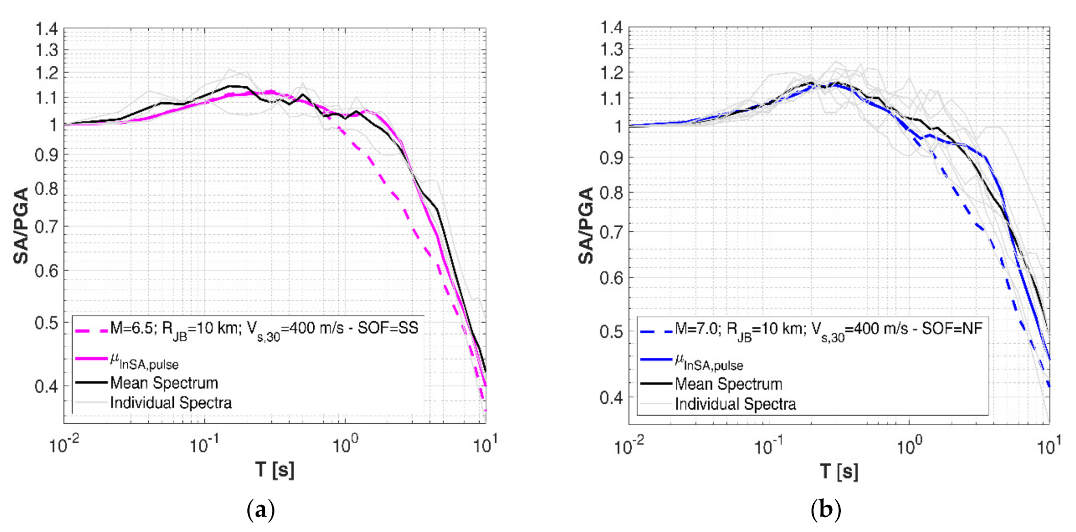
An example of model application for prediction adjustment is illustrated in Figure 11, which shows the average GMM (dashed lines) and the one modified by the amplification factor µ_lnAf,D50 (solid-colored lines) according to Equation (12) for two scenarios, compared to the observed spectral valuesfrom NESS1 dataset and divided by their PGA.

The first example scenario refers to M6.5 from SS faulting and site characterized by V_S,30 = 400 m/s and R_JB 10 km (Figure 11a); the second scenario is identical to the first one, except for the event that is M7.0 from NF rupture (Figure 11b).

The real observed SA values used for comparison are selected according to the same model parameters (magnitude and SOF) but with varying distance R_JB < 20 km and site properties V_S,30 = 400 ± 50 m/s. In these examples, the values of T_p used to calculate µ_lnAf,FN are estimated from Equation (1) calibrated on the pulse-like waveforms of NESS1 dataset.

Looking at Figure 11, it can be noted that the adjusted GMM is able to capture the peculiar mean shape of the selected spectra, in particular the characteristic “bump” that occurs on impulsive spectra at a period close to T_p.

6. Conclusions

In this paper we have shown the most relevant features of spectral response related to records affected by forward-directivity effects and calibrated a model for impulsive ground motions based on an empirical corrective factor.

In detail, the main findings of the presented study include: (i) observations on the statistical features of pulse-like acceleration and displacement elastic spectra, (ii) a new near-source ground-motion model (GMM) of ordinary (no pulse) near-fault records and (iii) a new narrow-band amplification factor of elastic acceleration response that accounts for the increased seismic demand due to pulse-like effects. The analysis and the models here proposed have been calibrated on a comprehensive and high-quality public dataset collecting metadata of near-source waveforms from moderate-to-large worldwide events (NESS1).

Our results confirm that pulse-like effects on acceleration response spectra are not negligible, particularly at higher periods close to the pulse-period. The effect is also evident on displacement spectra, both in terms of amplitudes and period range. The proposed near-source GMM is specifically calibrated on the subset of not-impulsive records, in order to remove any potential bias. The proposed model, used in conjunction with the amplification factor calibrated on the within-event part of the model residuals, allows predicting acceleration spectral response accounting for near-fault pulse-like directivity effects. The model could then be used in combination with contour maps of the probability of pulse occurrence of sites near fault ruptures (e.g., Shahi and Baker [10]; Chioccarelli and Iervolino [9]; Iervolino and Cornell [35]) for PSHA purposes, depending on source-to-site geometrical parameters [23].

The authors are currently investigating deeper the significance of pulse motions on displacement spectra to calibrate new models and adjustment factors, by using processed waveforms with a baseline correction scheme. Such a modeling could be usefully applied in the framework of performance-based design applications.

References

- Bolt, B.A.; Abrahamson, N.A. Estimation of strong seismic ground motions. In International Handbook of Earthquake and Engineering Seismology; Lee, W.H.K., Kanamori, H., Jennings, P.C., Kisslinger, C., Eds.; Academic Press: London, UK, 2003; pp. 983–1001. [Google Scholar]
- Mavroeidis, G.P.; Papageorgiou, A.S. A Mathematical Representation of Near-Fault Ground Motions. Bull. Seismol. Soc. Am. 2003, 93, 1099–1131. [Google Scholar] [CrossRef]
- Kalkan, E.; Kunnath, S.K. Effects of fling step and forward directivity on seismic response of buildings. Earthq. Spectra 2006, 22, 367–390. [Google Scholar] [CrossRef]
- D’Amico, M.; Felicetta, C.; Schiappapietra, E.; Pacor, F.; Gallovič, F.; Paolucci, R.; Sgobba, S.; Luzi, L. Fling Effects from Near-Source Strong-Motion Records: Insights from the 2016 M w 6.5 Norcia, Central Italy, Earthquake. Seismol. Res. Lett. 2019, 90, 659–671. [Google Scholar] [CrossRef]
- Somerville, P.G.; Smith, N.F.; Graves, R.W.; Abrahamson, N.A. Modification of Empirical Strong Ground Motion Attenuation Relations to Include the Amplitude and Duration Effects of Rupture Directivity. Seismol. Res. Lett. 1997, 68, 199–222. [Google Scholar] [CrossRef]
- Bray, J.D.; Rodriguez-Marek, A. Characterization of forward directivity ground motions in the near-fault region. Soil Dyn. Earthq. Eng. 2004, 24, 815–828. [Google Scholar] [CrossRef]
- Baker, J.W. Identification of Near-Fault Velocity Pulses and Prediction of Resulting Response Spectra. Proc. Geotech. Earthq. Eng. Struct. Dyn. IV 2009, 40975, 1–10. [Google Scholar]
- Tothong, P.; Cornell, C.A.; Baker, J.W. Explicit directivity-pulse inclusion in probabilistic seismic hazard analysis. Earthq. Spectra 2007, 23, 867–891. [Google Scholar] [CrossRef]
- Chioccarelli, E.; Iervolino, I. Near-source seismic demand and pulse-like records: A discussion for L’ Aquila earthquake. Earthq. Eng. Struct. Dyn. 2010, 39, 1039–1062. [Google Scholar] [CrossRef]
- Shahi, S.K.; Baker, J.W. An empirically calibrated framework for including the effects of near-fault directivity in probabilistic seismic hazard analysis. Bull. Seismol. Soc. Am. 2011, 101, 742–755. [Google Scholar] [CrossRef]
- Chang, Z.; Sun, X.; Zhai, C.; Zhao, J.X.; Xie, L. An empirical approach of accounting for the amplification effects induced by near-fault directivity. Bull. Earthq. Eng. 2018, 16, 1871–1885. [Google Scholar] [CrossRef]
- Akkar, S.; Moghimi, S.; Arıcı, Y. A study on major seismological and fault-site parameters affecting near-fault directivity ground-motion demands for strike-slip faulting for their possible inclusion in seismic design codes. Soil Dyn. Earthq. Eng. 2018, 104, 88–105. [Google Scholar] [CrossRef]
- Spudich, P.; Chiou, B.S.J. Directivity in NGA earthquake ground motions: Analysis using isochrone theory. Earthq. Spectra 2008, 24, 279–298. [Google Scholar] [CrossRef] [Green Version]
- Pacor, F.; Felicetta, C.; Lanzano, G.; Sgobba, S.; Puglia, R.; D’Amico, M.C.; Luzi, L. NEar-Source Strong-Motion Flatfile (NESS) (Version 1.0) [Data Set]; Istituto Nazionale di Geofisica e Vulcanologia (INGV): Rome, Italy, 2018. [Google Scholar] [CrossRef]
- Pacor, F.; Felicetta, C.; Lanzano, G.; Sgobba, S.; Puglia, R.; D’Amico, M.; Russo, E.; Baltzopoulos, G.; Iervolino, I. NESS1: A Worldwide Collection of Strong-Motion Data to Investigate Near-Source Effects. Seismol. Res. Lett. 2018, 89, 2299–2313. [Google Scholar] [CrossRef]
- D’Amico, M.; Felicetta, C.; Russo, E.; Sgobba, S.; Lanzano, G.; Pacor, F.; Luzi, L. Italian Accelerometric Archive v 3.1; Istituto Nazionale di Geofisica e Vulcanologia, Dipartimento della Protezione Civile Nazionale: Rome, Italy, 2020. [Google Scholar] [CrossRef]
- Luzi, L.; Lanzano, G.; Felicetta, C.; D’Amico, M.C.; Russo, E.; Sgobba, S.; Pacor, F. ORFEUS Working Group 5. Engineering Strong Motion Database (ESM) (Version 2.0); Istituto Nazionale di Geofisica e Vulcanologia (INGV): Rome, Italy, 2020. [Google Scholar] [CrossRef]
- Puglia, R.; Russo, E.; Luzi, L.; D’Amico, M.; Felicetta, C.; Pacor, F.; Lanzano, G. Strong-motion processing service: A tool to access and analyse earthquakes strong-motion waveforms. Bull. Earthq. Eng. 2018, 16, 2641–2651. [Google Scholar] [CrossRef]
- Baker, J.W. Quantitative classification of near-fault ground motions using wavelet analysis. Bull. Seismol. Soc. Am. 2007, 97, 1486–1501. [Google Scholar] [CrossRef]
- Boore, D.M. Orientation-independent, nongeometric-mean measures of seismic intensityfrom two horizontal components of motion. Bull. Seismol. Soc. Am. 2010, 100, 1830–1835. [Google Scholar] [CrossRef]
- Mavroeidis, G.P.; Dong, G.; Papageorgiou, A.S. Near-fault ground motions, and the response of elastic and inelastic singledegree-of-freedom (SDOF) systems. Earthq. Eng. Struct. Dyn. 2004, 33, 1023–1049. [Google Scholar] [CrossRef]
- Alavi, B.; Krawinkler, H. Behavior of moment-resisting frame structures subjected to near-fault ground motions. Earthq. Eng. Struct. Dyn. 2004, 33, 687–606. [Google Scholar] [CrossRef]
- Somerville, P.G. Magnitude scaling of the near fault rupture directivity pulse. Phys. Earth Planet 2003, 137, 201–212. [Google Scholar] [CrossRef]
- Somerville, P.G. Development of an improved representation of near fault ground motions. In Proceedings of the SMIP98 Seminar on Utilization of Strong Ground Motion Data, Oakland, CA, USA, 15 September 1998; pp. 1–20. [Google Scholar]
- Bates, D.; Mächler, M.; Bolker, B.; Walker, S. Fitting linear mixed-effects models using lme4. J. Stat. Softw. 2015, 67, 1–48. [Google Scholar] [CrossRef]
- Al-Atik, L.; Abrahamson, N.A.; Bommer, J.J.; Scherbaum, F.; Cotton, F.; Kuehn, N. The variability of ground-motion prediction models and its components. Seismol. Res. Lett. 2010, 81, 794–801. [Google Scholar] [CrossRef] [Green Version]
- Hubbard, D.T.; Mavroeidis, G.P. Damping coefficients for near-fault ground motion response spectra. Soil Dyn. Earthq. Eng. 2011, 31, 401–417. [Google Scholar] [CrossRef]
- Pu, W.; Kasai, K.; Kabando, E.K.; Huang, B. Evaluation of the damping modification factor for structures subjected to near-fault ground motions. Bull. Earthq. Eng. 2016, 14, 1519–1544. [Google Scholar] [CrossRef]
- Alonso-Rodríguez, A.; Miranda, E. Assessment of building behavior under near-fault pulse-like ground motions through simplified models. Soil Dyn. Earthq. Eng. 2015, 79, 47–58. [Google Scholar] [CrossRef]
- Liossatou, E.; Fardis, M. Near-fault effects on residual displacements of RC structures. Earthq. Eng. Struct. Dyn. 2016, 45, 1391–1409. [Google Scholar] [CrossRef]
- Cao, Y.; Mavroeidis, G.; Meza Fajardo, K.C.; Papageorgiou, A. Accidental eccentricity in symmetric buildings due to wave passage effects arising from near-fault pulse-like ground motions. Earthq. Eng. Struct. Dyn. 2017, 46, 2185–2207. [Google Scholar] [CrossRef]
- Baltzopoulos, G.; Iervolino, I.; Università degli Studi di Napoli, Federico II, Naples, Italy. Personal Communication, 2019.
- Cauzzi, C.; Faccioli, E.; Vanini, M.; Bianchini, A. Updated predictive equations for broadband (0.01–10 s) horizontal response spectra and peak ground motions, based on a global dataset of digital acceleration records. Bull. Earthq. Eng. 2015, 13, 1587–1612. [Google Scholar]
- Boore, D.M.; Atkinson, G.M. Ground-motion prediction equations for the average horizontal component of PGA, PGV, and 5%-damped PSA at spectral periods between 0.01 s and 10.0 s. Earthq. Spectra 2008, 24, 99–138. [Google Scholar] [CrossRef] [Green Version]
- Iervolino, I.; Cornell, C.A. Probability of Occurrence of Velocity Pulses in Near-Source Ground Motions. Bull. Seismol. Soc. Am. 2008, 98, 2262–2277. [Google Scholar] [CrossRef]
Figure 1.
Magnitude-distance distribution of the NESS1 records grouped by pulse-like and no-pulse records.
Figure 2.
Scatter plot of the pulse period Tp versus Magnitude along with the fitting function Equation (1); the Root-Mean-Squared_error RMSE is equal to 0.6043 and the statistical coefficient of determination R-square is 48.56% (a), relationship between pulse azimuth αpulse and strike normal angle αstrike90° for Strike-Slip (SS), Thrust-Fault (TF) and Normal-Fault (NF)—RMSE 172.2 and R-square 31% (b).
Figure 3.
Average elastic 5%-damped acceleration response spectra acceleration (SA) as RotD50 (a) and average elastic displacement spectra SD (b) in log-log scale, for pulse-like and no-pulse records in NESS1. Ratio between RotD50 and fault normal (FN) spectral components for acceleration (c) and displacement (d) elastic response spectra. Thin gray lines indicate the individual spectra; solid-colored lines refer to the mean of pulse-like records; the dashed lines refer to no-pulse records.
Figure 4.
Mean 5% damped acceleration response spectra SA divided by PGA (a) and displacement spectra SD (b) in log-log scale, grouped by 4 pulse period bins.
Figure 5.
Mean 5% damped acceleration response spectra divided by PGA (a) and displacement spectra (b) in log-log scale, grouped by styles of faulting (NF—Normal Fault; TF—Thrust Fault; SS—Strike Slip).
Figure 6.
Mean 5% damped acceleration spectra divided by PGA as predicted by the reference ground-motion model (GMM) (a) and related mean standard deviation σ (b) in log-log scale, for different distance metrics.
Figure 7.
Mean 5% damped acceleration spectra divided by PGA according to the reference GMM for RotD50 (a) and FN (b) components in log-log scale, compared to the mean of pulse-like spectra in NESS1.
Figure 8.
Individual and mean within-event residual values for pulse-like and no-pulse ground motions in NESS1.
Figure 9.
Normalized residuals ε of acceleration response spectra in NESS1 for RotD50 (a) and FN (b) pulse-like components.
Figure 10.
Amplification factor for spectral acceleration of pulse-like records compared to previous models [10,11,32,33,34].
Figure 11.
Observed and predicted SA according to the modified GMM for pulse-like ground motions (FN components), for two seismic scenarios: M6.5—SS type (a) and M7.0—NF type (b).
Publisher’s Note: MDPI stays neutral with regard to jurisdictional claims in published maps and institutional affiliations. |
© 2020 by the authors. Licensee MDPI, Basel, Switzerland. This article is an open access article distributed under the terms and conditions of the Creative Commons Attribution (CC BY) license (http://creativecommons.org/licenses/by/4.0/).
Share and Cite
MDPI and ACS Style
Sgobba, S.; Lanzano, G.; Pacor, F.; Felicetta, C. An Empirical Model to Account for Spectral Amplification of Pulse-Like Ground Motion Records. Geosciences 2021, 11, 15. https://0-doi-org.brum.beds.ac.uk/10.3390/geosciences11010015
AMA Style
Sgobba S, Lanzano G, Pacor F, Felicetta C. An Empirical Model to Account for Spectral Amplification of Pulse-Like Ground Motion Records. Geosciences. 2021; 11(1):15. https://0-doi-org.brum.beds.ac.uk/10.3390/geosciences11010015
Chicago/Turabian StyleSgobba, Sara, Giovanni Lanzano, Francesca Pacor, and Chiara Felicetta. 2021. "An Empirical Model to Account for Spectral Amplification of Pulse-Like Ground Motion Records" Geosciences 11, no. 1: 15. https://0-doi-org.brum.beds.ac.uk/10.3390/geosciences11010015
Note that from the first issue of 2016, this journal uses article numbers instead of page numbers. See further details here.