Article

Extreme Rainfall over Complex Terrain: An Application of the Linear Model of Orographic Precipitation to a Case Study in the Italian Pre-Alps

Department of Civil and Environmental Engineering, Politecnico di Milano, Piazza Leonardo da Vinci, 32, 20133 Milano, Italy
*
Author to whom correspondence should be addressed.
Submission received: 30 October 2020 / Revised: 21 December 2020 / Accepted: 28 December 2020 / Published: 31 December 2020

Abstract

:
Intense meteorological events are the primary cause of geohazard phenomena in mountain areas. In this paper, we present a study of the intense rainfall event that occurred in the provinces of Lecco and Sondrio from 11 to 12 June 2019. The aim of our work is to understand the effect of local topography on the spatial distribution of rainfall and to attempt the reconstruction of a realistic rainfall field relative to that extreme event. This task represents a challenge in the context of complex orography. Classical rain-gauge interpolation techniques, such as Kriging, may be too approximate, while meteorological models can be complex and often unable to accurately predict rainfall extremes. For these reasons, we tested the linear upslope model (LUM) designed for estimating rainfall records in orographic precipitation. This model explicitly addresses the dependence of rainfall intensification caused by the terrain elevation. In our case study, the available radio sounding data identified the convective nature of the event with a sustained and moist southern flow directed northward across the Pre-Alps, resulting in an orographic uplift. The simulation was conducted along a smoothed elevation profile of the local orography. The result was a reliable reconstruction of the rainfall field, validated with the ground-based rain gauge data. The error analysis revealed a good performance of the LUM with a realistic description of the interaction between the airflow and local orography. The areas subjected to rainfall extremes were correctly identified, confirming the determinant role of complex terrain in precipitation intensification.

1. Introduction

In alpine environments, hydrogeological hazards are mainly triggered by heavy rainfall events that can occur across the seasons in different ways [1,2,3]. The autumn is the most critical season, where extratropical cyclone structures can strike the alpine range frequently, affecting its southern flank slope [4,5,6]. These episodes can cause extensive damage, injuries, and deaths due to the possible triggering of critical events, such as floods and landslides [7,8]. In the literature, several approaches have been adopted to better understand the cause–effect relation between heavy rainfall and hydrogeological issues.
One of the most important is the elaboration of the intensity–duration curves where precipitation features are intended as predictors for the event triggering. These curves correlate the intensity and the duration of a precipitation event, defining a critical rainfall event with respect to a threshold above which landslide failures are highly expected [9,10,11,12,13]. For floods and flash floods, the event intensity is assessed through the evaluation of the correspondent return period of the rainfall, under the hypothesis of iso-frequency among floods and precipitation [1,4,5,6,14,15]. As a result, the information acquired about rainfall characteristics is fundamental for the correct assessment of these hydrogeological events.
All these approaches have different levels of approximation but require high quality input data. These data are retrieved from rain gauges time series. Unfortunately, rain gauges networks are not always uniformly spatially distributed, and they only provide single-point information. To overcome this limitation, compromises are adopted to deal with ungauged areas. In some cases, the nearest rain gauge is taken into account directly; however, more generally, a rainfall field is reconstructed from a station network, applying automatic interpolation methods, such as the Inverse Distance Weighted (IDW) or Kriging methods [16,17,18,19,20].
Interpolation techniques work well across flat areas where the terrain elevation is nearly constant or very smooth [18]. The simplest ones, such as IDW, are geometry-based where interpolated values depend only on the rain gauge distance. In this case, the availability of a sufficiently dense network is necessary to obtain a reasonable interpolation; however, this is sometimes not possible in mountain environments. The dependence of the rainfall field on elevation is not taken into account. In this light, geostatistical techniques, such as Kriging External Driven (KED) may be a viable solution: the classical Kriging could be conditioned (driven) considering an external drift, such as the elevation [18,21,22].
KED yields good results when a strong relationship between a meteorological variable and elevation is present. The spatial interpolation of temperature is an example of a successful application of KED [23,24]; however, this cannot be extended to precipitation. Precipitation follows neither an additive error model nor a Gaussian distribution (typical of temperatures), which are both prerequisites for a rigorous application of most geostatistical methods [18,25]. Instead, precipitation follows a multiplicative error model, and its distribution is positively skewed [25,26]. Therefore, the Kriging performances are low, especially in the reconstruction of daily and sub-daily rainfall fields.
To avoid these problems, several authors have proposed extensions of these interpolation methods. One is the PRISM model (Parameter Elevation Regressions on Independent slopes Models) [27,28,29]. The former is based on a weighted climate–elevation regression function that acknowledges the dominant influence of elevation on precipitation. To operate, for each meteorological station, there are assigned weights that account for other physiographical factors in addition to elevation, such as the topographic exposure or coastal proximity, which affect the climate at a variety of scales. The PRISM model was widely tested all over the world for other meteorological parameters, obtaining good responses by the scientific community for climatic data interpretation [28,29,30].
However, the PRISM model was not successfully applied to interpret localized events, such as the orographic thunderstorm triggered in watershed basins [31]. In these cases, Limited Area Models (LAMs) for local weather forecasting represent an important data source [5,14,31,32,33]. Their affordability is still increasing worldwide particularly in now-casting meteorology, and they are continuously updated and trained in the prediction of atmosphere dynamics [31,32]. Historically, one of the main drawbacks of these models has been the complexity of their parameterization regarding the cloud microphysics, which is the “engine” responsible for the formation of precipitation [5,31,32].
Difficulties have risen across mountain areas where the morphology could dramatically influence the rainfall processes, even at a local level [34]. Result variability is also dependent on the microphysical scheme implemented inside the model [5]. Currently, according to [35], the lack of predictability after a few hours represents a current challenge aspect for small-scale precipitation events. In particular, for scales smaller than ~60 km, predictability is lost rapidly within the first 6 h of the forecast, which is the typical scale length of the intense precipitation phenomena. For this reason, the design and the use of a convection-permitting ensemble appears promising [35,36]. However, also in these cases, meteorological outputs should be always compared and validated through appropriate error analysis with rain gauges records on the ground [14,25,26].
Bearing in mind that a unique technique to determine rainfall amounts for ungauged regions does not exist, especially for remote places in mountain territories, we focused on a model able to reconstruct a reliable rainfall field. The aim of our study was to attempt to overcome the poor accuracy of classical interpolation techniques, while avoiding the complexities of running a LAM. For these reasons, we tested the application of the “linear upslope model” (LUM) of orographic precipitation proposed by [37,38,39,40]. Three aspects drove our choice:
the rigorous but rather simple mathematical formulation that is inspired by the complex physics of meteorological models;
the flexible applicability that required limited spatial data, such as the local morphology, i.e., elevation, and available radiosonde data [31,40]; and
the extreme event of orographic rainfall that was recorded in the case study area.
The idea behind the linear upslope model is to reproduce, with sufficient accuracy, the mechanism of rainfall over complex morphology without considering the cloud microphysics. In our case study, we experimented with a typical situation of orographic precipitation where the territory of the provinces of Lecco and Sondrio (Figure 1) experienced an average rainfall depth of 110 mm in 13 h [41], with an extreme that reached 210 mm. That episode suggested the application of LUM. The aims were twofold: to better understand the role of orography in rainfall intensification and to reproduce a realistic rainfall field for the considered area.
The model is described in detail in the Materials and Methods section together with a presentation of the case study. In the Results section, we first present an elaboration of the radiosonde parameters used for model initialization, followed by the outcomes of the rainfall field reconstruction and an error analysis regarding the rain gauge measurements. Finally, our Discussion and Conclusion of the back-analysis study are reported with our comments.

2. Materials and Methods

2.1. The Linear Upslope Model (LUM)

LUM evaluates the spatial evolution of a precipitation P (mm) triggered by the local orography h (m). The idea behind the model formulation is the following: when a humid airflow rises along a slope, it starts to condense, cooling adiabatically and triggering rainfall on the up-slope flank of the mountain range. Beyond the mountain peak, the airflow begins to descend and dries out due to adiabatic warming, causing a decrease in rainfall. This simple conceptualization neglects all the cloud microphysics and airflow dynamics that characterize the complex atmosphere interaction with the local orography. For example, the perturbation of airflow trajectories after crossing a mountain peak are not explicitly simulated by the model; however, the water vapor depletion due to generated rainfall is taken into account [37,40].
P is expressed as a function of only two terms: the Water Vapour Flux and the local terrain slope. Water Vapour Flux (WVF) is an indicator of the airmass moisture and represents the integrated flux of water substance across vertical section of the atmosphere [39,40]. The WVF module is expressed in kg s−1 m−1 and is computed as:
| W V F | = 0 ρ q v | U ( z ) | d z ,
where ρ is the air density kg/m3, qv is the specific humidity %, and U(z) is the horizontal component of the wind vector m/s retrieved from balloon sounding where atmospheric parameters are measured with altitude. U(z) attributes the direction to the WVF vector.
The airflow evolution across space is described by the atmosphere continuity equation (Equation (2)) where the horizontal divergence of Water Vapour Flux vector (WVF) is equal to the difference among two terms: the precipitation P, that depletes WVF, and the surface evaporation E (mm), that refills WVF.
· W V F = P E .
Under the hypothesis of a steady state and a mono-dimensional airflow directed along positive x-axes, the WVF module can be expressed simply as a function of the spatial coordinate x. Equation (2) can be rewritten as Equation (3) making explicit the change of the WVF module along an x-path in two different locations, A and B [40]:
| W V F A | | W V F B | = A B P d x A B E d x   .
The P and E components can be expressed as a function of the WVF vector. Following the assumption proposed by [37,39], an airflow can rise up a mountain flank following the same slope as the underlying terrain. The airflow exhibits a vertical wind velocity, W, as a function of the horizontal component U(z) and terrain slope. Bearing in mind the mono-dimensional approximation, the elevation h is represented by a profile h(x) along the positive x direction.
W ( x , z ) = U ( z ) · d h ( x ) d x .
If the airflow rises following a moist-adiabatic lapse rate, i.e., a temperature gradient of around 6.5 °C/1000 m, and it is mostly saturated at all levels, the condensation rate, CR, kg s−1 m−1 can be evaluated as the vertical integral of the wind velocity W(x,z) m/s, the air density at saturation ρsat kg/m3, and the saturation scale height H s a t 1 m−1.
C R ( x ) = 0 [ 1 ρ s a t d ρ s a t d z ] ρ s a t ( z ) | U ( z ) | · d h ( x ) d x d z ,
1 ρ s a t d ρ s a t d z L γ R T 0 2 = H s a t 1 .
The saturation scale height H s a t 1 for water vapour ascending moist-adiabatically is approximated using the Clausius–Clapeyron theory, and can be expressed as a function of the latent heat of water, L = 2.5 × 10⁶ J kg−1, the gas constant for vapour RV = 461 J kg−1 K−1, the temperature at the ground T0 ≅ 20 °C = 293 K, and the moist-adiabatic lapse rate, γ.
Adjusting the previous Equation (5b), the precipitation rate, P, can be rewritten from the CR as in Equation (6) highlighting its dependence from the WVF vector and the terrain slope. Equation (6) states that, if the terrain elevation is increasing in the direction of the incoming upslope wind, the condensation of the air mass can generate precipitation in that area.
P ( x ) = H s a t 1 | W V F | · d h ( x ) d x   when   d h ( x ) d x > 0 .
On the other hand, when the WVF vector is approaching the downslope, the contribution due to the gradient is the opposite and the air mass tends to evaporate, due to the adiabatic warming (Equation (7)).
E ( x ) = H s a t 1 | W V F | · d h ( x ) d x             when   d h ( x ) d x < 0 .
LUM was implemented following these steps:
  • An initial condition of WVF vector was defined to initialize the model at coordinate x = 0.
  • Considering the local slope evaluated from the elevation profile and the WVF vector, P and E were estimated using Equations (6) and (7).
  • The continuity equation (Equation (3)) was considered to retrieve the new value of the WVF vector at coordinate x > 0.
  • The operation at points 2 and 3 was repeated until the end of the elevation profile.
The mechanism depicted by LUM is rather realistic even though simplified. The suitability has been tested on several occasions by authors who applied the methodology to different domains all over the world [37,38,39,40].

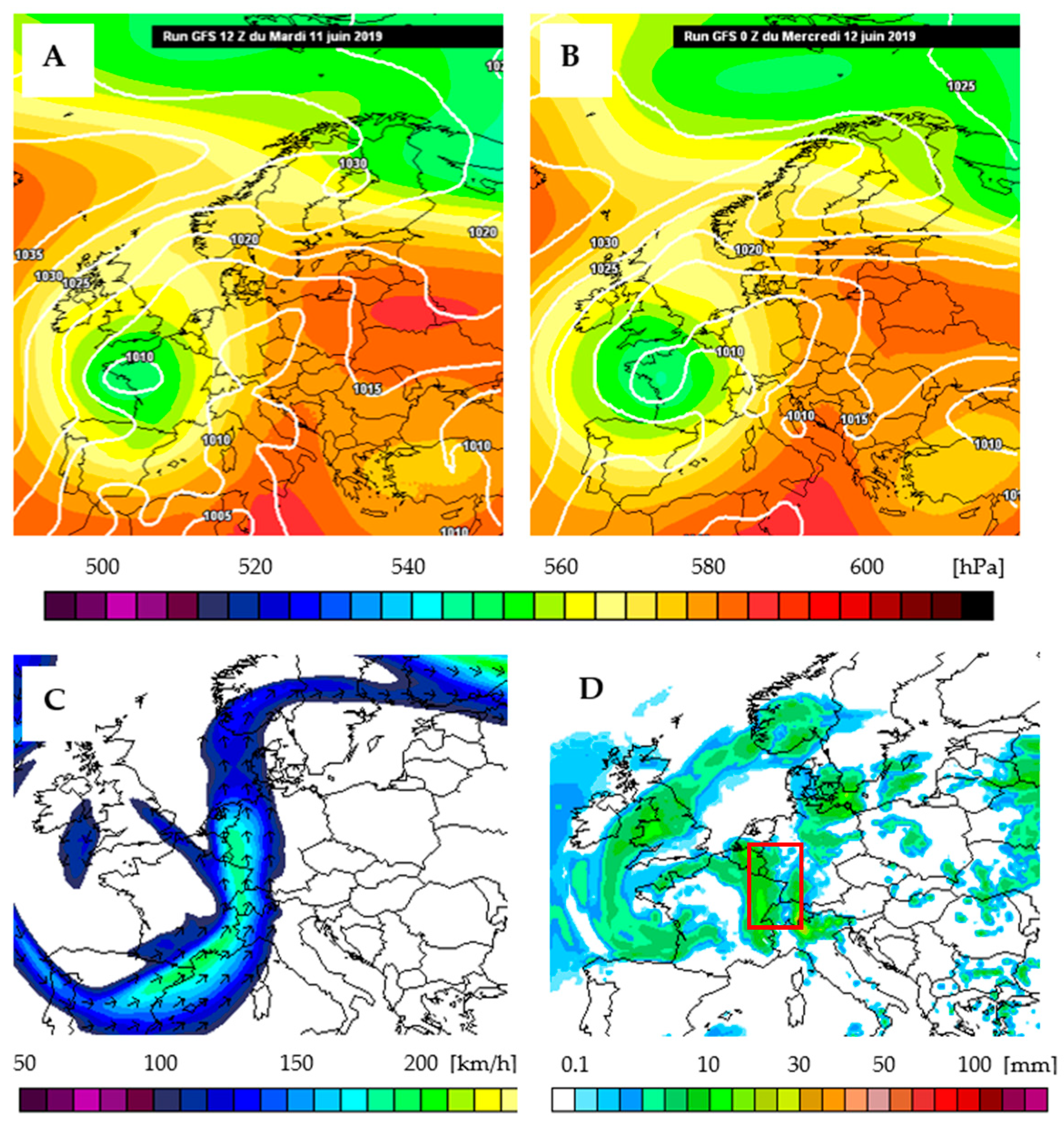
2.2. The Case Study of 11–12 June 2019

During the night between 11 and 12 June 2019, an extreme convective rainfall event occurred in the upper part of the Lake of Como, affecting the territory of the provinces of Lecco and Sondrio (Figure 1). Rather persistent and auto-regenerating thunderstorms started during the evening of 11 June around 8 p.m. and did not dissipate completely until 9 a.m. the following day. A huge amount of rainfall fell with an average rainfall depth of 110 mm in 13 h [41]. The town of Premana experienced a total of 210 mm in 13 h that corresponds to a precipitation with a return period of 200 years. This datum has been estimated considering the local “Intensity–Duration–Frequency” (IDF) from [41]. All rainfall depths recorded in the study area and reported from local environment agency ARPA Lombardia [41] are listed in Table 1. Figure 1A,B depict the location of the study area in the Lecco and Sondrio Provinces (Lombardy Region, Italy) and the local rain gauge network from Arpa Lombardia.
This event caused serious damage. As shown in Figure 1, thunderstorms followed a narrow corridor path along a south–north section, striking the area near the town of Premana. Due to the extreme precipitation, a sudden flash flood in the Varrone river hit Dervio, a town located downstream to Premana. The Pagnona dam risked a dam break due to the reservoir overtopping, and thus Dervio’s inhabitants were temporarily sheltered. In Sondrio province, several shallow landslides and debris flows affected the slopes of Mount Legnone in the municipality of Delebio and Piantedo, and a road in the S. Giacomo Filippo municipality collapsed due to Liro river flood.
All these events happened in the same area and in a relatively short time. For these reasons, particular attention was posed to the analysis of meteorological maps of that episode [42]. Looking at a regional scale, the position of air masses in Figure 2A,B show a low pressure centred on western France. This configuration was responsible of the warm and humid air advection coming from Mediterranean Sea in the direction of the central sector of the Alps. The temporal persistency of heavy rainfalls was caused by the stationarity behaviour of the air masses that were not advected eastward faster as it is typically seen during a thunderstorm episode (Figure 2A,B shows a not appreciable difference over 12 h).
That humid airflow was also sustained by the presence of intense jet streams as reported in Figure 2C. The core velocities reached values around 180–190 km/h at 300 hPa geopotential height contributing to increasing the air upslope motions due to upper layer divergence [5,43]. The straight path followed by rainfall extreme events depicted in Figure 1B is, therefore, defined by the upstream currents that advected thunderstorm cells northward (Figure 2C,D).
The exceptionality of this event could be explained only considering the local effect of orography on airflow motion. According to [4,6,24,30,34], two more meteorological forcings were identified as responsible for that intensity. The first regards the local low-level convergence of moist southerly flows as reported in Figure 3, which shows wind trajectories and velocities at 2000 m. The second is the presence of the orographic barrier of Orobie Alps (Figure 1) that was hit by an incoming southerly flow triggering the upslope movement of airmasses. These two elements were simulated in more detail considering the linear upslope model presented.

3. Results

In this section, the application of the LUM to the case study is reported. In the first and second part, the initial conditions of LUM were retrieved from radiosonde data, and hypotheses on model applicability are discussed. In the third part, the model results are validated through error analysis comparing with rain gauge recordings.

3.1. Convective Nature of the Rainfall Event

Radiosondes are a valuable instrument for the exhaustive definition of the 3D structure of the atmosphere [5,31,32]. They are equipped with a small aerostatic balloon and launched every 12 h from selected sites around the globe. These balloons carry a small box containing meteorological sensors for the vertical profiling [46] of quantities, such as the pressure (hPa), elevation (m), temperature (°C), relative humidity (%), dew point temperature (°C), wind velocity (m/s), and wind direction (°).
In our case study, sounding data collected near the Linate Milan Airport (60 km distance from Lecco, shown in Figure 1) were provided by University of Wyoming [46]. Two radio soundings were examined: the 12 h UTC of 11 June and the 00 h UTC of 12 June (Figure 4). The first was intended as a precursor of the atmosphere state favourable to trigger the extreme rainfall. The second was indeed representative of the airflow dynamic that occurred during the rainfall. Therefore, both soundings were used for assessing the initial condition WVF0 for LUM.
To facilitate the interpretation of the atmosphere state, convective parameters, such as CAPE, CIN, and LI ([5,34,47]), and height parameters, such as LCL, LFC, and EL ([5,32,34]) have been retrieved from radio soundings:
CAPE is the acronym of Convective Available Potential Energy, and it is an indicator of atmospheric instability, a necessary condition severe weather hazard.
CIN stands for Convective Inhibition and represents the amount of energy required to overcome the negatively buoyant energy that the environment exerts on an air parcel. The latter is not the opposite of CAPE, but the two indexes give complementary information: when CAPE is high, above 1000 J kg−1 and CIN is low, less −30 J kg−1, the probability of convective triggering is high.
LI (Lifted Index) is the temperature difference between the environment Te and air parcel lifted adiabatically Tp at a given pressure height, usually 500 hPa.
LCL is the Level of Condensation and represents the height where the cloud formation is started.
LFC (Level of Free Convection) is the height where the air parcel can rise-up without external forces and thunderstorms systems can form.
EL (Equilibrium Layer) is the height where vertical motion is stopped and generally corresponds to the thunderstorm cap or anvil.
The values reported in Table 2 confirm the instability conditions of the atmosphere column. This fact is highlighted primarily by Brunt–Vaisala frequency N2, which assumes negative values [5,32].
Looking at the convective parameters, the first sounding is the most critical. The former exhibits the highest CAPE and the lowest CIN, which correspond to conditions of “moderate” instability. LI is low, depicting a situation where severe storms with strong lifting mechanisms have a high probability to occur. The second sounding exhibits lower values of CAPE and LI and higher values of CIN since the thunderstorms have been already triggered and have started to dissipate the atmosphere energy.
Considering the height parameters, the thunderstorm-prone structure of the atmosphere can be well recognized. Comparing the two soundings, this configuration remained stationary for 12 h, confirming the previous hypothesis coming from air masses analysis. The LCL was settled slightly above the upper boundary layer limit, and the LFC was around 2000 m, at the top of the mountain peaks of the Orobie Alps. Therefore, convective cells could have been triggered easily above the mountain range and evolved freely up to the EL that was settled around 10 km.
In summary, the convective nature of the extreme rainfall event was clearly described by the radio sounding even if located slightly far away from the area studied. All the analysed parameters indicated the instability of the atmosphere but were not sufficient to explain the severity of the phenomena recorded over the Alps. The soundings data provide us with two essential parameters required by LUM: the initial conditions and the precipitation efficiency ratio.

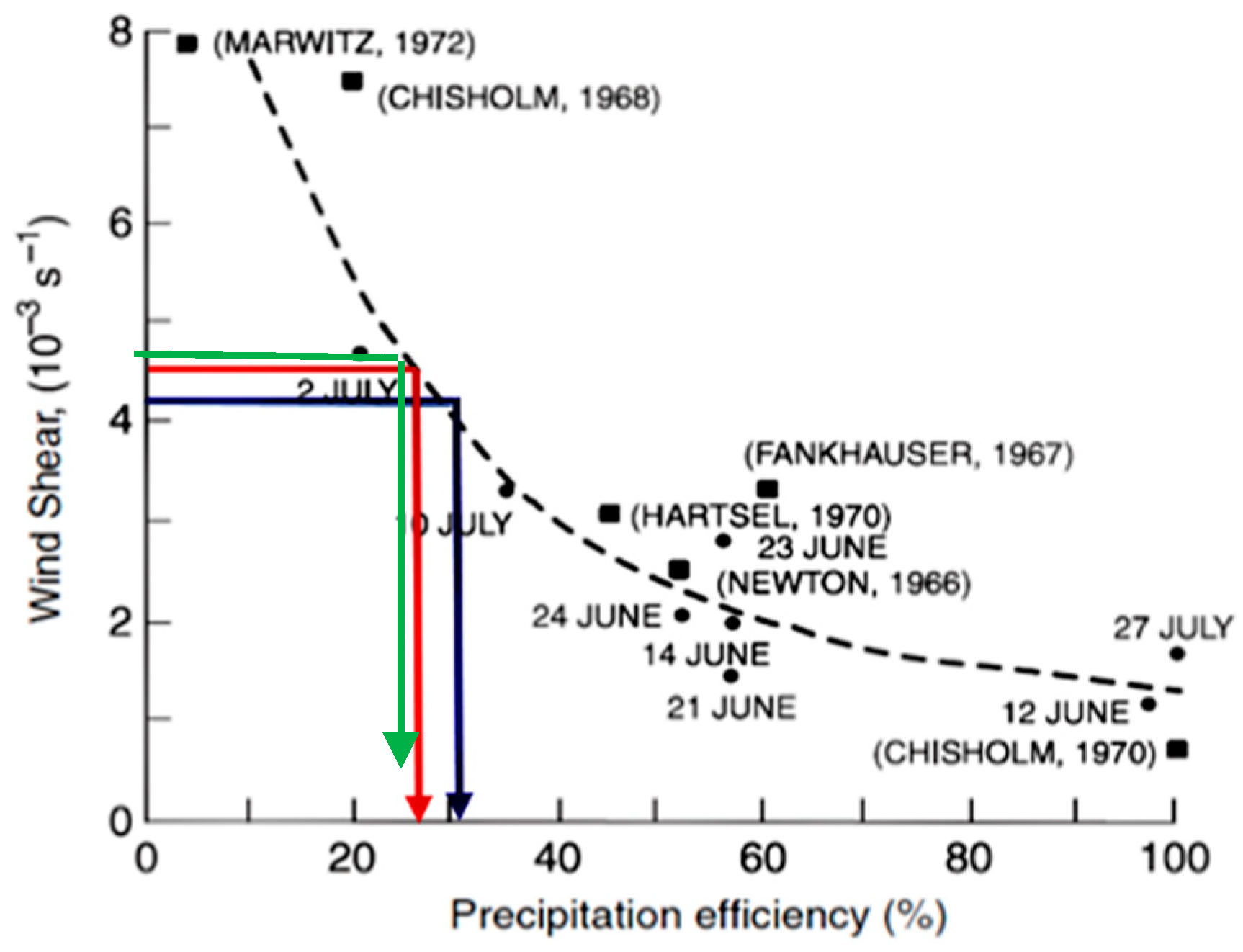
3.2. The Initial Conditions and the Precipitation Efficiency Ratio

The continuity equation of LUM (Equations (2) and (3)) requires an initial condition. As specified in the Materials and Methods section, we described the model under two hypotheses: a steady state condition and a mono-dimensional geometry along the x coordinate. Therefore, the initial condition for the incoming airflow is defined by the vector WVF0 calculated at location x = 0. Looking at Table 3, the WVF0 vector was retrieved for each sounding described previously, plus a third one recorded on 12 June 2019 12 h UTC.
As reported in Equation (4), the module of WVF vector is represented by the integral over an air column height. The integral limits were assessed looking at the sounding data: they were comprised between the LCL (lower) and EL (upper) levels. For each sounding, validity windows were defined as 6 h backward and 6 h forward from the central reference time. Then, considering that the rainfall event started at 8 p.m. of 11 June until 9 a.m. of 12 June, the two soundings of 12 June 2019 00 h UTC and 12 June 2019 12 h UTC were selected to compute the average module of WVF0 at location x = 0.
Inside LUM, the microphysics of rainfall processes is not explicitly considered since an instantaneous transformation between condensate quantity in the cloud (CR) and rain, P is assumed [31,39,40]. Therefore, a correction term should be introduced to take into account the efficiency of these processes that can significantly reduce the effective rainfall amount [48]. The precipitation efficiency, Ep, is expressed as the ratio of the Patm, rainfall computed by a generic atmospheric model and Pgauge, the rainfall recorded by rain gauges on the ground:
E p = P g a u g e P a t m
P g a u g e = E p P a t m
Several authors correlated Ep with different parameters of radio sounding, and a rather useful relationship can be found considering the wind shear. The former represents the wind velocity difference between the ground and a reference height of 6000 m [5,32]. Using the relationship proposed by [48] in Figure 5, from the three-radio sounding, a reasonable precipitation efficiency value was assessed to be around 0.3 (Table 4).

3.3. Linear Upslope Model Applied to the Case Study

The application of the LUM to our case study required further simplifications to make the problem more tractable. The first regards the mono-dimensional approximation of the domain geometry. The event analysis has depicted a clear south–north corridor followed by thunderstorms (Figure 1). That rectilinear path can ideally define a bidimensional domain that slices the atmosphere along the horizontal and vertical coordinates x and z. Bearing in mind that the quantity WVF is vertically integrated, the problem is reduced to one dimension.
For an accurate representation of the ground elevation h along the thunderstorm path depicted in Figure 1, a group of five parallel traces was extracted from a Digital Elevation Model (DEM). The DEM has a 5 m cell resolution and was freely downloaded from geoportal of Lombardy Region [49]. The obtained traces were then averaged in a unique profile to derive a representative value of h(x) along the south–north section. As reported by [31,37,40,50], the LUM results were not well correlated with very detailed DEMs. The airflow was generally not sensitive to a local abrupt slope change but was instead conditioned by the average height field. Consequently, we resampled the original DEM at a coarser resolution of 500 m to obtain a smoother representation of the local terrain orography.
Inside the LUM, the presence of the boundary layer (BL) near the ground was not explicitly taken into consideration. BL is a portion of airmass that tends to be at rest in contrast to the free atmosphere [5,32]. The height of BL is difficult to estimate with a closed formulation as it depends on several variables and has a typical diurnal cycle [5,32,34,51,52]. It tends to be completely depleted after intense rainy events due to the increased turbulence caused by downdrafts [53,54]. We included this parameter in our simulation, nevertheless. Using the soundings data and looking at temperature inversion in proximity of the ground, the BL height was estimated. As shown in Table 5, the diurnal fluctuation of the BL was in the order of 1000 m, and this represents the range considered for the study.
The BL was included in the LUM formulation proposing a new elevation profile that can differ significantly from the real terrain. In particular, the areas settled under the BL height were automatically flattened because they were assumed to be excluded from rainfall formation processes. Figure 6 shows the comparison between the real terrain profile and the adjusted one considering BL. A reference value of boundary layer of 1000 m was adopted for the Val Padana side, and an indicative value of 600 m was used for the Valtellina floodplain. The latter was decreased considering the possibility that local valley winds are responsible for its rapid depletion [31,52,55].
After these considerations and adjustments, LUM was applied to the case study. The continuity equation was integrated explicitly to evaluate the variation of P(x) and E(x) along the northward direction x. The spatial evolution of the WVF vector exhibited a depletion of 55% after the transit over the mountain region. The WVF0 were around 540 kg s−1 m−1 near Lecco, and its final value dropped down to 260 kg s−1 m−1 near the Spluga Pass, 75 km northward.
In Figure 7, the spatial evolution of P (blue) and E (red) cumulated over 13 h are reported. Comparing the graph with the elevation profile, it could be highlighted that LUM works in accordance with the physics of the orographic rainfall mechanism that led to precipitation formation in the windward portion of the mountain (upslope) and the evaporation in the lee side (downslope). This is particularly evident for Mount Legnone, which is the highest peak of the entire cross section (1500 m smoothed and 2650 m effective).
The LUM results of P(x) and E(x) appear to be physically correct; however, we noticed that the rainfall amounts were under/overestimated at certain points and rather irregularly distributed. Therefore, to obtain a realistic representation of the rainfall pattern, a smoothing function was applied to P(x). We tested three different smoothing windows related to the meso-gamma scale of the studied phenomena: 5, 10, and 20 km ranges, as reported in Figure 8. We considered a smoothing window of 10 km that better fit the observed values. This also led us to believe that 10 km was the length scale of the thunderstorms that occurred in the region during the event [5,32,53]. The green continuous line in Figure 7 and Figure 8 represents the smoothed function for the precipitation P(x): the values of the rainfall field are now more uniformly distributed with respect to the initial prediction (Figure 7). The results have already considered the reduction ratio related to the precipitation efficiency (0.3).
In Figure 9A,B, the rain-gauge amounts of the nearest weather station were plotted against the rainfall profile, showing a good accordance among the two datasets. The highest value recorded at the Premana rain gauge was well represented by LUM, indicating that in the surrounding area the upslope motion of the air likely conditioned the dynamic of the incoming WVF flux significantly.
In Table 6, we report the error quantifications of the smoothed rainfall field with respect to the reference rain gauge stations located along the profile. The absolute error was generally confined around few millimetres of rain, with a maximum of 40 mm across the Valtellina flood plain. Looking at the relative errors, an average was assessed at nearly 20%, which is rather low considering the model adopted and its approximations. At the point of Premana, a small error (around 30 mm) with respect to the total rainfall amount was estimated.

4. Discussion

As we have seen from the results listed in Table 6, the errors were maintained under control with respect to the reference rain gauges, giving a realistic reconstruction of the rainfall field. In contrast to the classical interpolation techniques, we also gained a physical interpretation of the phenomena under twofold aspects. The first regards the analysis of the soundings data that can depict the atmosphere state before and during the event, highlighting potential critical situations, as in the present case. The second consists of a better understanding of orographic rainfall mechanism in relation to several parameters that can influence it. We can say that LUM can be more “didactic” compared with complex LAM models, and its simple implementation permits making the problem more tractable.
One of the strengths is the relatively small amount of input data required for the implementation. A lack of data is generally a problem in mountain catchments; however, as we have seen in our case study, the LUM was correctly initialized using only the sounding data and topographic elevation. Unfortunately, even if the terrain elevation is available worldwide with good resolution, sounding data are typically single-point data. In this particular case, the radio soundings were taken some 60 km away from the starting point of the simulation. This approximation was considered acceptable for defining the initial conditions of the model, i.e., the WVF0.
The estimation of WFV0, could be a non-trivial task at some locations or even not sufficiently precise to feed the linear model. It is more likely that the sounding is located too far away from the studied area, i.e., hundreds of kilometres. In that case, the atmosphere’s vertical profile should be inferred through comparing different data sources, especially considering the vertical atmosphere profiles retrieved from reanalysis models or using satellites. The information detected by infrared sensors and LiDAR scanners from geostationary satellites are now providing encouraging results in terms of WVF estimation. These techniques are currently adopted for the study of atmospheric rivers [56,57]. As a matter of fact, increasing the data availability regarding atmospheric moisture flows may help in this way.
Another point of discussion concerns the hypothesis of linearity under which the model operates. In fact, trying to represent or simulate a chaotic system, such as the atmosphere, with a liner model could appear as nonsense. In our view, this is partially true. As described by the model authors, the model contains a strong simplification of the processes occurring in the atmosphere. Microphysics is completely neglected, and rainfall formation is reduced to a simple water mass balance of the WVF flow. This is clearly not true in reality, and the process is simulated by LAM. The complexity of LAMs sometimes does not permit effective control of the solution especially over complex terrain and when the orography abruptly influences the rainfall generation. LUM permitted us to highlight the critical parameters that affect the final outcome of the model, neglecting second-order influences. In the case study, the test of LUM moved on in this direction, accepting some simplification but sill presenting a reasonable rainfall field reconstruction. These simplifications are discussed here in detail:
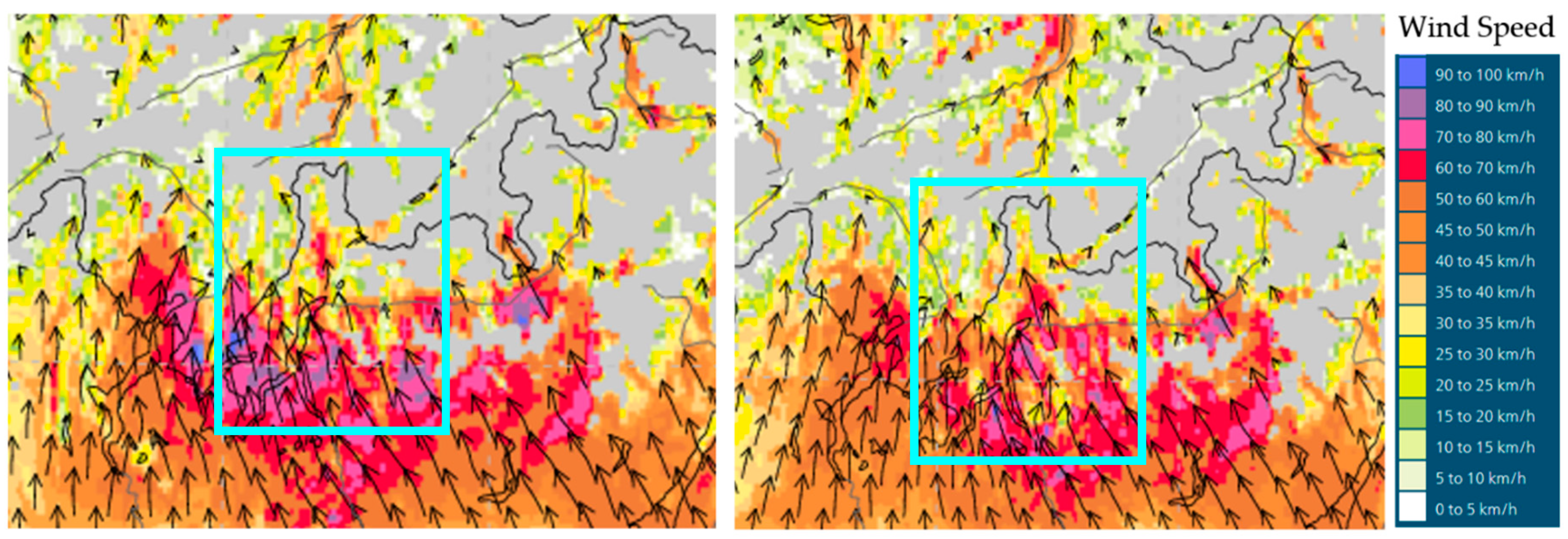
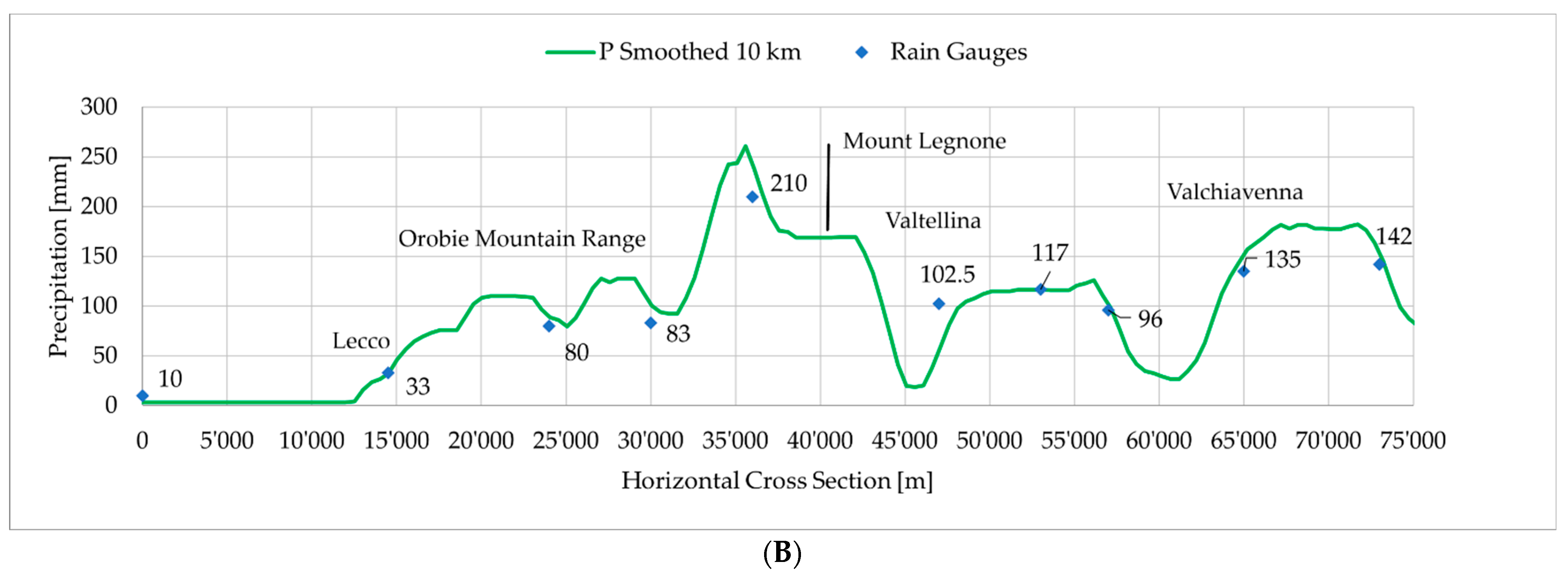
The mono-dimensional domain is a strong idealization of the event that occurred. The sounding data compared to a local LAM depicted an event that developed northward following a narrow cone extension. The thunderstorm corridor had a clear starting point, an average width around 10–15 km but to an extent of 100 km. Therefore, also considering the low-level wind convergence (Figure 3), a mono-dimensional reduction was sufficiently realistic.
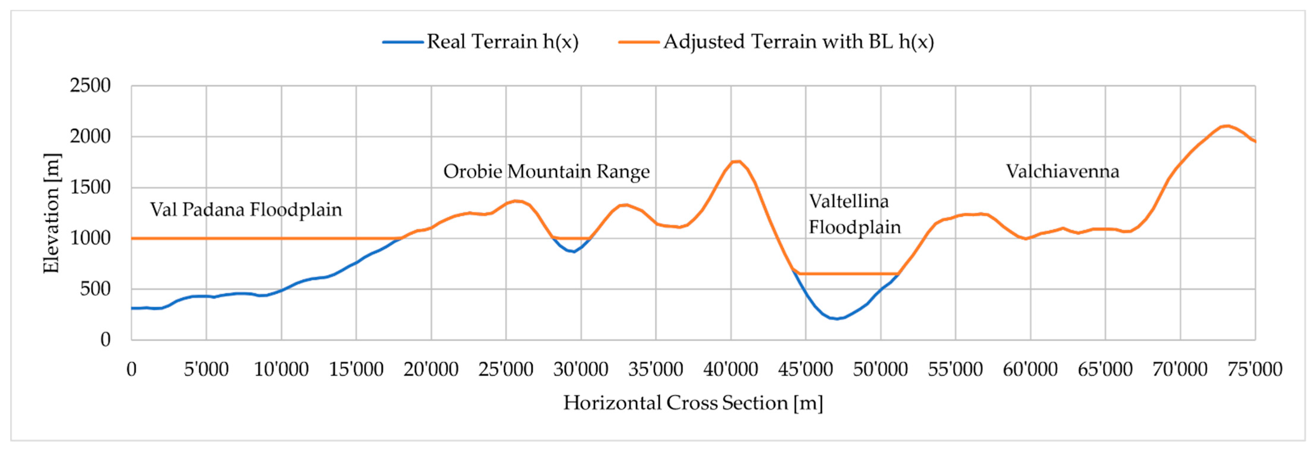
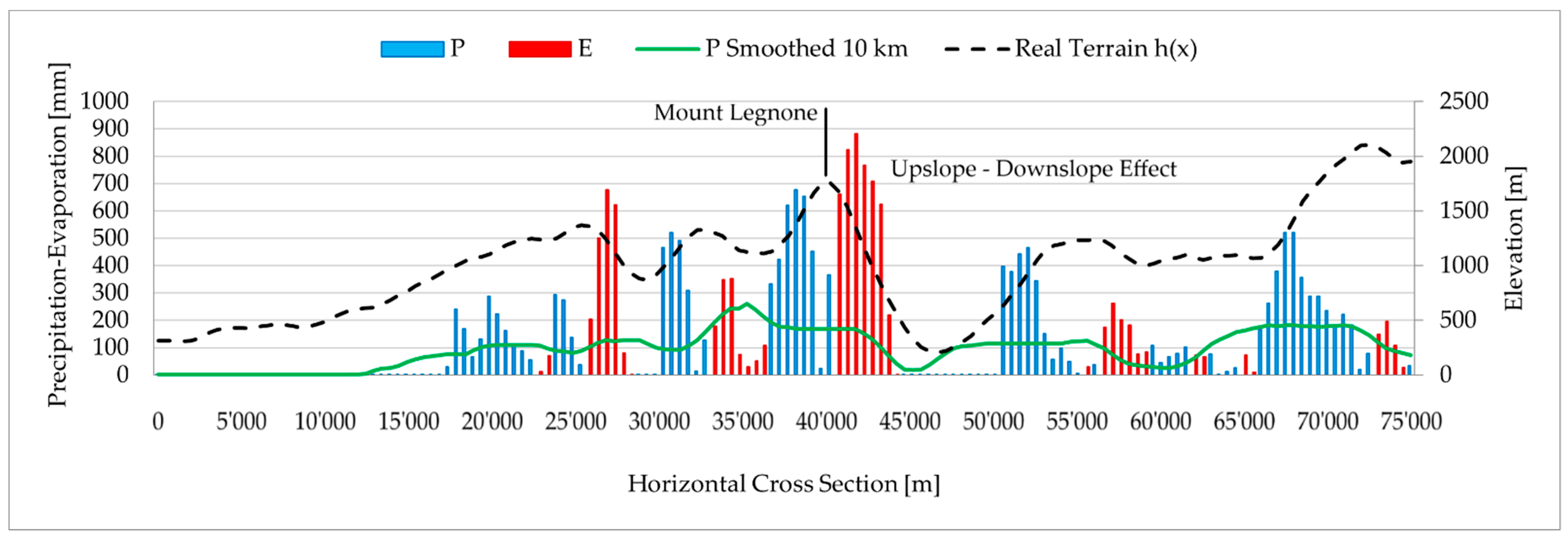
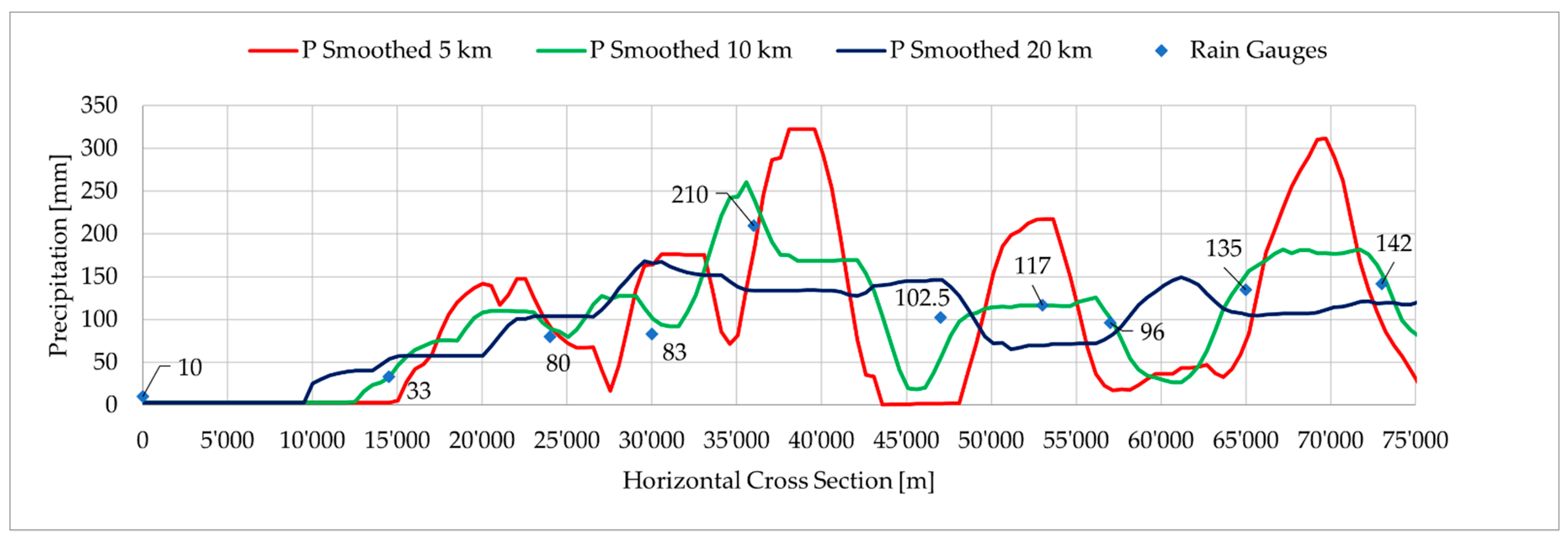
The resampling of orography is an operation that is generally adopted in atmospheric models. For the Alps, a rectangular shape range with a 2000 m average slope was considered in the past as a sufficient representation of the morphology in regional atmospheric-dynamic models [6,32,34,50]. Currently, LAMs can assimilate orography at higher resolutions, but the smoothing operations are still necessary [58,59]. In our case, the high sensitivity of LUM to the terrain profile required that the local morphology be smoothed to obtain realistic simulations.
The topographic influence on incoming airflow can generate gravity waves and turbulences that can also perturb the airflow dynamic along the vertical [5,34,60]. These secondary effects likely played a significant role in the spatial redistribution of the rainfall, especially behind the peak of Mount Legnone where the results showed the highest errors with underestimation of around 40 mm. Using the linear model, the airmass uplift triggered by orography was the predominantly simulated process, and the others were confined to the second order. For these reasons, the downslope dynamics are poorly described due to high non-linearities that may occur in these processes.
The estimation of the boundary layer height cannot be computed explicitly, and this represents a significant uncertainty that should be treated carefully. However, in our opinion, this quantity should be considered when LUM is adopted. As we determined for this case study, BL was essential to determine the portion of the atmosphere that can contribute to the effective rainfall generation. The motivation is the following: due to surface friction, low atmosphere layers are maintained at rest and do not experience any upslope motion until the BL is completely eroded. In our case study, the evidence was confirmed looking at three sounding data where, for layers comprised in BL, the wind velocities were sensibly reduced, and their directions were not aligned with the WFV airflow. If these layers are included in the computation of WFV0, they could lead to a sensible overestimation of the initial conditions due to their high concentration in water vapour. For these reasons, we tested this BL adjustment, and the results demonstrated good improvements in the LUM simulation.
Bearing in mind these necessary simplifications, the final result was rather encouraging. The model highlighted how the orography played a determinant role in intensifying the precipitation rate locally. As was observed in analysing the reconstructed precipitation field, the critical value recorded at Premana rain gauge was matched correctly. In the upper part of Valchiavenna, the model outcome was in good accordance with the rain gauge measurements. Likely, hidden errors were also contained in the reference rain gauges, particularly due to their relative distance from the cross section considered, such as in the case of Barzio station. For this reason, an extension of LUM for working with 2D domains could be a further improvement of the analysis to fulfil these uncertainties. We concluded that the linear upslope model produced a reliable reproduction of this exceptional rainfall event.

5. Conclusions

The aim of this paper was to reconstruct a realistic rainfall field through the application of a simple linear upslope model. Over complex terrain, this task is required in many fields, in particular for hydrogeological risk assessment. Interpolation techniques that consider only the data recorded by rain gauge networks may fail as they do not consider orography as critical factor for precipitation intensification. On the other hand, LAMs offer a good solution to investigate rainfalls; however, their complexity is highly data-demanding, and, especially in mountain environments, solutions could often be too approximate.
For these reasons, we attempted to apply the linear upslope model proposed by [37], which represents an intermediate alternative. To test the model application, a case study was chosen due to its severity, which was intensified by two main causes: the favourable meteorological conditions of the atmosphere and the interaction with the local orography. Considering the known limitations and the simplification adopted, LUM was determined to be suitable for the purpose.
The rainfall field reconstruction was able to fit the data obtained from the reference rain gauges, particularly around the critical areas where the highest amount of rainfall was recorded. In addition, this allowed us to increase our understanding of this type of complex meteorological phenomena, discovering the importance of BL for the assessment of the initial conditions related to the WVF vector. Consequently, the role of airflow interactions with orographic terrain was more clearly depicted in relation to the extreme localized rainfall, which was able to trigger several hydrogeological hazards. In this light, LUM represents a valuable instrument for a rapid but comprehensive analysis, Water Vapour Flux as demonstrated in this critical case study.

Author Contributions

Conceptualization, A.A. and L.L.; Data curation, A.A. and L.L.; Formal analysis, A.A.; Investigation, A.A.; Methodology, A.A. and L.L.; Supervision, L.L.; Validation, L.L. and M.P.; Visualization, M.P.; Writing—original draft, A.A.; Writing—review & editing, L.L. and M.P. All authors have read and agreed to the published version of the manuscript.

Funding

This research was partially funded by Fondazione Cariplo, grant number 2017-0722.

Informed Consent Statement

Informed consent was obtained from all subjects involved in the study.

Data Availability Statement

Publicly available datasets were analyzed in this study. Data references can be found in bibliography where website URLs are specified.

Acknowledgments

We are grateful to Raffaele Copes and Giovanni Scaramella who contributed to this work during the development of their thesis.

Conflicts of Interest

The authors declare no conflict of interest.

References

  1. Longoni, L.; Ivanov, V.I.; Brambilla, D.; Radice, A.; Papini, M. Analysis of the temporal and spatial scales of soil erosion and transport in a Mountain Basin. Ital. J. Eng. Geol. Environ. 2016, 16, 17–30. [Google Scholar] [CrossRef]
  2. Gariano, S.L.; Guzzetti, F. Landslides in a changing climate. Earth Sci. Rev. 2016, 162, 227–252. [Google Scholar] [CrossRef] [Green Version]
  3. Papini, M.; Ivanov, V.; Brambilla, D.; Arosio, D.; Longoni, L. Monitoring bedload sediment transport in a pre-Alpine river: An experimental method. Rend. Online Della Soc. Geol. Ital. 2017, 43, 57–63. [Google Scholar] [CrossRef]
  4. Grazzini, F. Predictability of a large-scale flow conducive to extreme precipitation over the western Alps. Meteorol. Atmos. Phys. 2007, 95, 123–138. [Google Scholar] [CrossRef]
  5. Stull, R.B. Practical Meteorology: An Algebra-Based Survey of Atmospheric Science; University of British Columbia: Vancouver, BC, Canada, 2017. [Google Scholar]
  6. Rotunno, R.; Houze, R. Lessons on orographic precipitation for the Mesoscale Alpine Programme. Q. J. R. Meteorol. Soc. 2007, 133, 811–830. [Google Scholar] [CrossRef]
  7. Ozturk, U.; Tarakegn, Y.; Longoni, L.; Brambilla, D.; Papini, M.; Jensen, J. A simplified early-warning system for imminent landslide prediction based on failure index fragility curves developed through numerical analysis. Geomat. Nat. Hazards Risk 2015, 7, 1406–1425. [Google Scholar] [CrossRef] [Green Version]
  8. Albano, R.; Mancusi, L.; Abbate, A. Improving flood risk analysis for effectively supporting the implementation of flood risk management plans: The case study of “Serio” Valley. Environ. Sci. Policy 2017, 75, 158–172. [Google Scholar] [CrossRef]
  9. Guzzetti, F.; Peruccacci, S.; Rossi, M.; Stark, C.P. The rainfall intensity–duration control of shallow landslides and debris flows: An update. Landslides 2008, 5, 3–17. [Google Scholar] [CrossRef]
  10. Longoni, L.; Papini, M.; Arosio, D.; Zanzi, L. On the definition of rainfall thresholds for diffuse landslides. Trans. State Art Sci. Eng. 2011, 53, 27–41. [Google Scholar] [CrossRef] [Green Version]
  11. Ciccarese, G.; Mulas, M.; Alberoni, P.P.; Truffelli, G.; Corsini, A. Debris flows rainfall thresholds in the Apennines of Emilia-Romagna (Italy) derived by the analysis of recent severe rainstorms events and regional meteorological data. Geomorphology 2020, 358, 107097. [Google Scholar] [CrossRef]
  12. Caine, N. The Rainfall Intensity: Duration Control of Shallow Landslides and Debris Flows. Geogr. Ann. Ser. Phys. Geogr. 1980, 62, 23–27. [Google Scholar] [CrossRef]
  13. Ivanov, V.; Arosio, D.; Tresoldi, G.; Hojat, A.; Zanzi, L.; Papini, M.; Longoni, L. Investigation on the Role of Water for the Stability of Shallow Landslides-Insights from Experimental Tests. Water 2020, 12, 1203. [Google Scholar] [CrossRef] [Green Version]
  14. Martin, J.E. Mid-Latitude Atmosphere Dynamics; Wiley: Chichester, West Sussex, UK, 2006. [Google Scholar]
  15. Ivanov, V.; Radice, A.; Papini, M.; Longoni, L. Event-scale pebble mobility observed by RFID tracking in a pre-Alpine stream: A field laboratory. Earth Surf. Process. Landf. 2020, 45, 535–547. [Google Scholar] [CrossRef]
  16. Tao, T.; Chocat, B.; Liu, S.; Xin, K. Uncertainty Analysis of Interpolation Methods in Rainfall Spatial Distribution-A Case of Small Catchment in Lyon. J. Water Resour. Prot. 2009, 2, 136–144. [Google Scholar] [CrossRef] [Green Version]
  17. Chen, T.; Ren, L.; Yuan, F.; Yang, X.; Jiang, S.; Tang, T.; Liu, Y.; Zhao, C.; Zhang, L. Comparison of Spatial Interpolation Schemes for Rainfall Data and Application in Hydrological Modeling. Water 2017, 9, 342. [Google Scholar] [CrossRef] [Green Version]
  18. Ly, S.; Charles, C.; Degre, A. Different methods for spatial interpolation of rainfall data for operational hydrology and hydrological modeling at watershed scale. A review. Biotechnol. Agron. Soc. Environ. 2013, 17, 392–406. [Google Scholar]
  19. Jacquin, A.; Soto-Sandoval, J. Interpolation of monthly precipitation amounts in mountainous catchments with sparse precipitation networks. Chil. J. Agric. Res. 2013, 73, 406–413. [Google Scholar] [CrossRef] [Green Version]
  20. Di Piazza, A.; Conti, F.; Viola, F.; Eccel, E.; Noto, L. Comparative Analysis of Spatial Interpolation Methods in the Mediterranean Area: Application to Temperature in Sicily. Water 2015, 7, 1866–1888. [Google Scholar] [CrossRef] [Green Version]
  21. Hengl, T.; Heuvelink, G.; Stein, A. Comparison of Kriging with External Drift and Regression-Kriging; Tech. Note; ITC: Enschede, The Netherlands, 2003. [Google Scholar]
  22. Bourennane, H.; King, D.; Couturier, A. Comparison of kriging with external drift and simple linear regression for predicting soil horizon thickness with different sample densities. Geoderma 2000, 97, 255–271. [Google Scholar] [CrossRef]
  23. Hudson, G.; Wackernagel, H. Mapping temperature using kriging with external drift: Theory and an example from scotland. Int. J. Climatol. 1994, 14, 77–91. [Google Scholar] [CrossRef]
  24. Varentsov, M.; Esau, I.; Wolf, T. High-Resolution Temperature Mapping by Geostatistical Kriging with External Drift from Large-Eddy Simulations. Mon. Weather Rev. 2020, 148, 1029–1048. [Google Scholar] [CrossRef]
  25. Tian, Y.; Huffman, G.J.; Adler, R.F.; Tang, L.; Sapiano, M.; Maggioni, V.; Wu, H. Modeling errors in daily precipitation measurements: Additive or multiplicative? Geophys. Res. Lett. 2013, 40, 2060–2065. [Google Scholar] [CrossRef] [Green Version]
  26. Brownlees, C.; Cipollini, F.; Gallo, G. Multiplicative Error Models. In Handbook of Volatility Models and Their Applications; John Wiley & Sons: Hoboken, NJ, USA, 2011. [Google Scholar] [CrossRef] [Green Version]
  27. Daly, C.; Taylor, G.; Gibson, W. The PRISM Approach to Mapping Precipitation and Temperature. In Proceeding of the 10th AMS Conference Applied Climatology, Reno, NV, USA, 18–25 October 1997; pp. 20–23. [Google Scholar]
  28. Daly, C.; Slater, M.E.; Roberti, J.A.; Laseter, S.H.; Swift, L.W., Jr. High-resolution precipitation mapping in a mountainous watershed: Ground truth for evaluating uncertainty in a national precipitation dataset. Int. J. Climatol. 2017, 37, 124–137. [Google Scholar] [CrossRef] [Green Version]
  29. Jeong, H.-G.; Ahn, J.-B.; Lee, J.; Shim, K.-M.; Jung, M.-P. Improvement of daily precipitation estimations using PRISM with inverse-distance weighting. Theor. Appl. Climatol. 2020, 139, 923–934. [Google Scholar] [CrossRef] [Green Version]
  30. Chen, D.; Ou, T.; Gong, L.; Xu, C.-Y.; Li, W.; Ho, C.-H.; Qian, W. Spatial interpolation of daily precipitation in China: 1951–2005. Adv. Atmos. Sci. 2010, 27, 1221–1232. [Google Scholar] [CrossRef]
  31. Barry, R.G. Mountain Weater and Climate, 3rd ed.; Cambridge University Press: Cambridge, UK, 2008. [Google Scholar]
  32. Wallace, J.M.; Hobbs, P.V. Atmospheric Science: An Introductory Survey; Elsevier: Oxford, UK, 2006. [Google Scholar]
  33. Cotton, W.R.; Bryan, G.H.; Van Den Heever, S.C. Cumulonimbus Clouds and Severe Convective Storms. In Storm and Cloud Dynamics; Elsevier: London, UK, 2011. [Google Scholar]
  34. Kirshbaum, D.; Adler, B.; Kalthoff, N.; Barthlott, C.; Serafin, S. Moist Orographic Convection: Physical Mechanisms and Links to Surface-Exchange Processes. Atmosphere 2018, 9, 80. [Google Scholar] [CrossRef] [Green Version]
  35. Frogner, I.-L.; Singleton, A.T.; Køltzow, M.Ø.; Andrae, U. Convection-permitting ensembles: Challenges related to their design and use. Q. J. R. Meteorol. Soc. 2019, 145, 90–106. [Google Scholar] [CrossRef] [Green Version]
  36. Coppola, E.; Sobolowski, S.; Pichelli, E.; Raffaele, F.; Ahrens, B.; Anders, I.; Ban, N.; Bastin, S.; Belda, M.; Belusic, D.; et al. A first-of-its-kind multi-model convection permitting ensemble for investigating convective phenomena over Europe and the Mediterranean. Clim. Dyn. 2020, 55, 3–34. [Google Scholar] [CrossRef]
  37. Smith, R.B.; Barstad, I. A Linear Theory of Orographic Precipitation. J. Atmos. Sci. 2004, 61, 1377–1391. [Google Scholar] [CrossRef]
  38. Smith, R. A linear time-delay model of orographic precipitation. J. Hydrol. 2003, 282, 2–9. [Google Scholar] [CrossRef]
  39. Smith, R.B. The Influence of Mountains on the Atmosphere. In Advances in Geophysics; Saltzman, B., Ed.; Elsevier: Oxford, UK, 1979; Volume 21, pp. 87–230. ISBN 0065-2687. [Google Scholar]
  40. Smith, R.B. 100 Years of Progress on Mountain Meteorology Research. Meteorol. Monogr. 2018, 59, 20.1–20.73. [Google Scholar] [CrossRef]
  41. ARPA Lombardia Rete Monitoraggio Idro-Nivo-Meteorologico. Available online: www.arpalombardia.it/stiti/arpalombardia/meteo (accessed on 1 September 2020).
  42. Kalnay, E.; Kanamitsu, M.; Kistler, R.; Collins, W.; Deaven, D.; Gandin, L.; Iredell, M.; Saha, S.; White, G.; Woollen, J.; et al. The NCEP/NCAR 40-Year Reanalysis Project. Bull. Am. Meteorol. Soc. 1996, 77, 437–472. [Google Scholar] [CrossRef] [Green Version]
  43. Grazzini, F.; Vitart, F. Atmospheric predictability and Rossby wave packets. Q. J. R. Meteorol. Soc. 2015, 141, 2793–2802. [Google Scholar] [CrossRef]
  44. MeteoCiel Observations, Prévisions, Modèles en Temps Réel. Available online: www.meteociel.fr (accessed on 1 September 2020).
  45. Meteo Swiss Meteo Swiss Waether Overview. Available online: https://www.meteoswiss.admin.ch/home.html?tab=overview (accessed on 12 June 2019).
  46. University of Wayoming Upperair Air Data. Available online: http://weather.uwyo.edu/upperair/sounding.html (accessed on 1 September 2020).
  47. NOAA National Center for Environmental Information. Available online: https://www.ncei.noaa.gov/ (accessed on 1 September 2020).
  48. Marwitz, J.D. Precipitation efficiency of thunderstorms on the high plains. Pascal Fr. Bibliogr. Databases 1972, 6, 367–370. [Google Scholar]
  49. Regione Lombardia Geoportale Regione Lombardia. Available online: https://www.geoportale.regione.lombardia.it/ (accessed on 30 October 2020).
  50. Caroletti, G.; Barstad, I. An assessment of future extreme precipitation in western Norway using a linear model. Hydrol. Earth Syst. Sci. 2010, 14. [Google Scholar] [CrossRef] [Green Version]
  51. Haghighi, E.; Shahraeeni, E.; Lehmann, P.; Or, D. Evaporation rates across a convective air boundary layer are dominated by diffusion. Water Resour. Res. 2013, 49, 1602–1610. [Google Scholar] [CrossRef] [Green Version]
  52. Serafin, S.; Adler, B.; Cuxart, J.; De Wekker, S.; Gohm, A.; Grisogono, B.; Kalthoff, N.; Kirshbaum, D.; Rotach, M.; Schmidli, J.; et al. Exchange Processes in the Atmospheric Boundary Layer over Mountainous Terrain. Atmosphere 2018, 9, 102. [Google Scholar] [CrossRef] [Green Version]
  53. Kessler, E. On the continuity and distribution of water substance in atmospheric circulations. Atmos. Res. 1995, 38, 109–145. [Google Scholar] [CrossRef]
  54. Ćurić, M. Numerical modeling of thunderstorm. Theor. Appl. Climatol. 1989, 40, 227–235. [Google Scholar] [CrossRef]
  55. Serafin, S.; Zardi, D. Structure of the Atmospheric Boundary Layer in the Vicinity of a Developing Upslope Flow System: A Numerical Model Study. J. Atmos. Sci. 2010, 67, 1171–1185. [Google Scholar] [CrossRef]
  56. Ralph, F.M.; Neiman, P.J.; Wick, G.A. Satellite and CALJET Aircraft Observations of Atmospheric Rivers over the Eastern North Pacific Ocean during the Winter of 1997/98. Mon. Weather Rev. 2004, 132, 1721–1745. [Google Scholar] [CrossRef] [Green Version]
  57. Gimeno, L.; Nieto, R.; Vázquez, M.; Lavers, D. Atmospheric rivers: A mini-review. Front. Earth Sci. 2014, 2, 2. [Google Scholar] [CrossRef]
  58. Rontu, L. Studies on Orographic Effects in a Numerical Weather Prediction Model. Master’s Thesis, University of Helsinki, Helsinki, Finland, 2013. [Google Scholar]
  59. Elvidge, A.D.; Sandu, I.; Wedi, N.; Vosper, S.B.; Zadra, A.; Boussetta, S.; Bouyssel, F.; van Niekerk, A.; Tolstykh, M.A.; Ujiie, M. Uncertainty in the Representation of Orography in Weather and Climate Models and Implications for Parameterized Drag. J. Adv. Model. Earth Syst. 2019, 11, 2567–2585. [Google Scholar] [CrossRef] [Green Version]
  60. Vallis, G.K. Essentials of Atmospheric and Oceanic Dynamics; Cambridge University Press: Cambridge, UK, 2019; ISBN 978-1-107-69279-4. [Google Scholar]
Figure 1. (A) The case study area in the Lecco and Sondrio Provinces (Lombardy Region, Italy) with affected municipalities and infrastructures; (B) the local rain gauges network from Arpa Lombardia with the south-north airflow direction along the thunderstorm path (dotted red line).
Geosciences 11 00018 g001
Figure 2. Meteorological reanalysis maps of the 11–12 June 2019 event [42,44]: (A,B) represent the pressure field at 500 hPa reference geopotential, respectively, at 20:00 of 11 June and 8:00 of 12 June; (C) depicts the upper divergence velocities of jet streams at 300 hPa reference geopotential, and (D) shows the rainfall field amounts on 12 June at 8:00 in Europe where higher values are visible across the study area depicted in the red box.
Geosciences 11 00018 g002
Figure 3. Low-level wind convergence (blue boxes) recorded in the study area at 2000 m, © Meteo Swiss [45], during the night of 12 June at 3:00 and 4:00.
Geosciences 11 00018 g003
Figure 4. Radio soundings of Milano Linate recorded at 12:00 UTC of 11 June (A) and at 00:00 UTC of 12 June (B) [46].
Geosciences 11 00018 g004
Figure 5. Precipitation efficiency as a function of the wind shear, modified after [48].
Geosciences 11 00018 g005
Figure 6. Adjustment of the terrain elevation profile considering the existence of boundary layer (BL).
Geosciences 11 00018 g006
Figure 7. Precipitation P and evaporation E distribution along the south–north cross section. The green line represents the smoothed precipitation field.
Geosciences 11 00018 g007
Figure 8. Smoothing windows tested for rainfall field reconstruction considering meso-gamma scale length of investigated phenomena.
Geosciences 11 00018 g008
Figure 9. (A) The precipitation field is represented against the orography of the area and (B) is compared with respect to the rain gauge measurements.
Geosciences 11 00018 g009aGeosciences 11 00018 g009b
Table 1. The rain gauge amount recorded in the study area from 8 p.m. 11 June to 9 p.m. 12 June.
Rain Gauge StationRainfall Cumulated (mm)Rain Gauge StationRainfall Cumulated (mm)
Montevecchia10Fuentes115
Lecco33Vercana97
Barzio80Samolaco96
Cortenova83Prata123
Premana210Gordona142
Colico 90San Giacomo107
Dubino121Campodolcino160
Verceia114Madesimo157
Table 2. Convective parameters of the two radio soundings considered.
11 June 2019 12:00 UTC12 June 2019 00:00 UTC
N2 (s−1)−0.00027−0.00024
Atmospheric Conditionunstableunstable
CAPE (J kg−1)1371.38386.24
CIN (J kg−1)−40.83−84.15
LI (°C)−4.52−2.78
LCL (hPa) (m)873.49 hPa (1218 m)869.00 hPa (1262 m)
LFC (hPa) (m)790.35 hPa (2049 m)763.20 hPa (2336 m)
EL (hPa) (m)273.18 hPa (10,879 m)332.52 hPa (8605 m)
Table 3. The Water Vapour Flux (WVF0) values considered as the initial conditions for the linear upslope model.
11 June 2019
12:00 UTC
12 June 2019
00:00 UTC
12 June 2019
12:00 UTC
Average
WFV0 [kg s1 m1]202610152540
Table 4. Wind shear and precipitation efficiency for the three radio soundings.
11 June 2019
12:00 UTC (Red)
12 June 2019
00:00 UTC (Blue)
12 June 2019
12:00 UTC (Green)
Wind Shear (10−3 s−1)4.41 4.254.37
Ep ()0.270.320.29
Table 5. The boundary layer height estimation for the three radio soundings.
11 June 2019 12 h UTC12 June 2019 00 h UTC12 June 2019 00 h UTC
Boundary Layer Height [m]15004001800
Table 6. Rain gauge comparison with model precipitation field and errors assessment.
Rain Gauge Stationx Terrain Coordinate (m)P Rain Gauge (mm)P Model (mm)
Montevecchia0105.0
Lecco14,5003332.8
Barzio24,0008088.8
Cortenova30,00083100.6
Premana36,000210238.6
Colico-Fuentes47,00010260.0
Dubino-Verceia53,000117116.0
Samolaco57,0009697.8
Gordona-Prata65,000135157.2
San Giacomo -Madesimo73,000142145.5
Absolute Error (mm)Relative Error (%)Root Mean Square Error (mm)
14.0219.7812.17
Publisher’s Note: MDPI stays neutral with regard to jurisdictional claims in published maps and institutional affiliations.

