Mapping Groundwater Seepage in a Fen Using Thermal Imaging


Harold Hamm School of Geology and Geological Engineering, University of North Dakota, Grand Forks, ND 58202, USA
*
Author to whom correspondence should be addressed.
Geosciences 2021, 11(1), 29; https://0-doi-org.brum.beds.ac.uk/10.3390/geosciences11010029
Submission received: 12 November 2020
/
Revised: 23 December 2020
/
Accepted: 3 January 2021
/
Published: 6 January 2021
Abstract
:The transport of dissolved minerals and groundwater flow plays a crucial role in the ecosystem of many wetlands. Nonetheless, installing equipment to monitor groundwater seepage is invasive, harms vegetation, and can impact biodiversity. By remotely mapping surface temperature in late summer, when there is the greatest difference between warm soil and cold groundwater, temperature patterns can expose areas with the greatest upward gradient and flow. The conventional method of using tensiometers to measure hydraulic gradient and estimate flux using Darcy’s law was applied and compared with thermal imaging to characterize groundwater seepage at two contrasting sites within a central North Dakota fen (groundwater discharge wetland). Both sites exhibited variable gradients between the shallow and deep tensiometers. The temperature trend determined from the thermal imaging showed a closer relationship to the measured hydraulic gradients at the herbaceous (Sedge) site than at the wooded (Willow) site. Saturated hydraulic conductivity K ranged from 6 × 10⁻⁵ to 2 × 10⁻⁴ m/s for the Willow site; and 6 × 10⁻⁶ to 1 × 10⁻⁴ m/s for Sedge site. The flux calculated for the Willow site ranged from 1.4 × 10⁻⁵ to 2.7 × 10⁻⁴ m/s and that of the Sedge site ranged from 2.2 × 10⁻⁶ to 6.3 × 10⁻⁵ m/s. The gradients are affected at shallow depth because of heterogeneous soil stratigraphy, which is likely the reason that seepage faces at the sites cannot be mapped solely by thermal imaging.
1. Introduction
Understanding the basic principles and dynamics of surface water–groundwater interaction helps to ensure proper management and conservation of global water resources. Mapping groundwater seepage zones in a wetland can provide information about the groundwater flow system and the potential transport of groundwater contaminants [1]. Water resource managers can determine the overall health of a wetland, its watershed, the connected aquifer and extent, and its water budget with a basic understanding of the surface water–groundwater interactions and its flow regime.
Characterizing groundwater flow at seepage faces is essential, as seepage faces are a potential source of groundwater discharge and contamination, and seepage influences the water budgets of watersheds, lakes, and streams. Groundwater flow or flux is the rate at which water seeps from groundwater (aquifer) to the surface and it is difficult to measure directly. Surface water and groundwater are connected in most landscapes [2]. Due to the exchange of water between surface water and groundwater, alteration in one will affect the other due to their connectivity [2,3]. The area to which groundwater discharges to the surface is referred to as the seepage zone and occurs in areas where there is an upward hydraulic gradient. Generally, in these areas of significant upward gradient, groundwater discharge creates wetlands and stream flow. Seepage zones create complex interactions between surface water and groundwater [3,4], where groundwater discharge occurs along the stream banks [3,4], well walls [5], hill slopes, shorelines [6], and in drainage canals where a sharp pressure gradient exists between the internal saturated zone and external seepage area [5]. Wetlands are not only found in low points and depressions on the landscape but also on slopes. Fens are wetlands that are commonly formed and maintained by discharge of groundwater seepage. Fens receive nutrients from sources other than precipitation, usually from upslope sources through drainage from surrounding mineral soils [7,8]. Wetland plants can be categorized into fibrous-root plants and thick-root plants. Fibrous-root plants are plants with many fine and long lateral roots, while thick-root plants have few extensive fine lateral roots [9]. Fibrous-root plants also have significantly higher root activity, photosynthetic rate, transpiration rate than thick-root plants, as described in Lai et al. [9]. Seepage zones are now recognized as an important path for water and nutrients from the groundwater to the surface [10,11] and are crucial to maintaining ecologically healthy streams [12] and wetlands.
Installation of field equipment to characterize the hydraulic gradient, hydraulic conductivity, and calculating groundwater flux in wetlands (here referred to as the conventional method), however, is time consuming, costly, intensive, and equipment intrusive. It can damage vegetation, potentially decrease biodiversity, and disrupt natural hydraulic conditions. Therefore, to conserve the wetland, nutrient source, and ecology, it is important to develop less invasive methods of mapping and characterizing groundwater seepage.
The aim of this research is to map groundwater seepage using thermal imaging and investigate the potential for using thermal imaging as a tool for locating and characterizing groundwater seepage, which can be accomplished without disturbing the soil profile and by eliminating the cost of installing monitoring equipment. This approach may provide a simple, noninvasive method to more thoroughly understand the groundwater system of wetlands without disturbing site hydrology, biota, or soil profile.
To achieve these research aims, two methods are applied to investigate a fen in central North Dakota. The first uses the conventional method of measuring groundwater flow direction and rate of flow. This will determine the groundwater flux and the flow direction (upward or downward) to evaluate the second method, which employs thermal imagery captured on the surface of the wetland using a thermal camera, coupled with thermal imagery acquired using an unmanned aerial vehicle (UAV). These methods are compared in relationship to their efficiency and accuracy.
Groundwater seepage zones are often significantly cooler in summer and warmer in winter than the water at the surface [3,13], making it possible to detect the outflow temperature difference by using thermal imaging. Since groundwater seepage has a thermal signature on the surface, it may be used to characterize the seepage in fens and show how it correlates with using conventional methods to characterize seepage.
1.1. Background
1.1.1. Temperature as a Groundwater Flow Indicator
Heat has been identified and used as a groundwater tracer [14]. Since groundwater temperature is relatively constant while surface water temperature varies on diurnal and seasonal cycles [5], the differences can be used as a tracer to map seepage. Heat carried by groundwater has been used as a tracer to identify surface water infiltration [3,14], indicate seepage dynamics, and zones of groundwater seepage [3]. Heat has been used to trace groundwater movement [1,5,12,13,14,15,16,17]. Many studies [3,5,14,18] have used heat as a groundwater tracer to study the flow system, flow direction, and recharge and discharge, and therefore potentially characterizing groundwater dynamics. Heat information offers the possibility to detect the movement of groundwater, and location of discharge, and therefore the distribution of groundwater flow that transitions to surface water [3,13,19].
1.1.2. Previous Research on Thermal Imaging of Groundwater Seepage
Thermal imaging detects infrared energy (heat) remotely and converts it into an electronic signal, which is then processed to produce a thermal image, on which you can perform temperature calculations. Thermal-infrared imagery has been proven to delineate groundwater seepage and has thermal signature on the surface water [1,3,6,12]. All temperature-based models take advantage of the fact that in seasonal climates groundwater has a smaller intra-annual temperature amplitude than surface water [13]. Ground-based thermal imagery is a simple, practical tool to discriminate between areas with snow cover, snow melt, water seepage, and stream water [17]. Distributed temperature sensors (DTS) have been used to detect concurrent spatial variability in discharge and make continuous measurements in time at the groundwater–surface water interface [16,19]. DTS systems are devices that measure temperatures by means of fiber-optic, which can be used in lake bottom, mine shaft, air-snow interface, air-water interface and in first-order streams [16,20]. The advantages of DTS compared to point measurement, such as forward-looking infrared thermal imaging (FLIR), which takes snapshots of temperature in time, is that the DTS takes continuous temperature measurements concurrently in many locations along the length of the cable. This is in contrast to single point measurements made at different times; DTS also can detect concurrent spatial variability in discharge, which may be missed in the point measurements. Regardless, DTS require installation and at least minimal disturbance if used in wetlands.
Thermal imaging has been used to map groundwater discharge, characterize seepage faces, and distinguish between areas of low, moderate, and high groundwater discharge at the seepage boundary [5]. A thermal image is best captured when there is minimal sun radiation to reduce heat absorption, which minimizes emissivity [5]. Due to the large temperature difference between groundwater and the surface water, based at certain times during seasonal cycles, Deitchman and Loheide [5] were able to identify groundwater seepage in a stream bank and drainage ditch environment.
Early and late summer is considered the best season for collection of thermal infrared imaging, when the temperature gradient between the surface water and groundwater are the greatest. Field observation are focused on times when solar radiation is minimal or not present [18], but when there is a significant thermal differential between the atmosphere and subsurface [5]. Thermal infrared imaging has been the most effective at locating and analyzing seeps when the temperature differential between groundwater and the ambient air temperature is large [18].
Thermal imaging can provide a less invasive and cost-effective technique for characterizing groundwater in wetlands, since it only requires the use of a thermal imaging camera to capture images on the ground. These data can be analyzed by identifying cold and hot spots and then mapping groundwater seepage areas.
1.1.3. Description of the Study Site
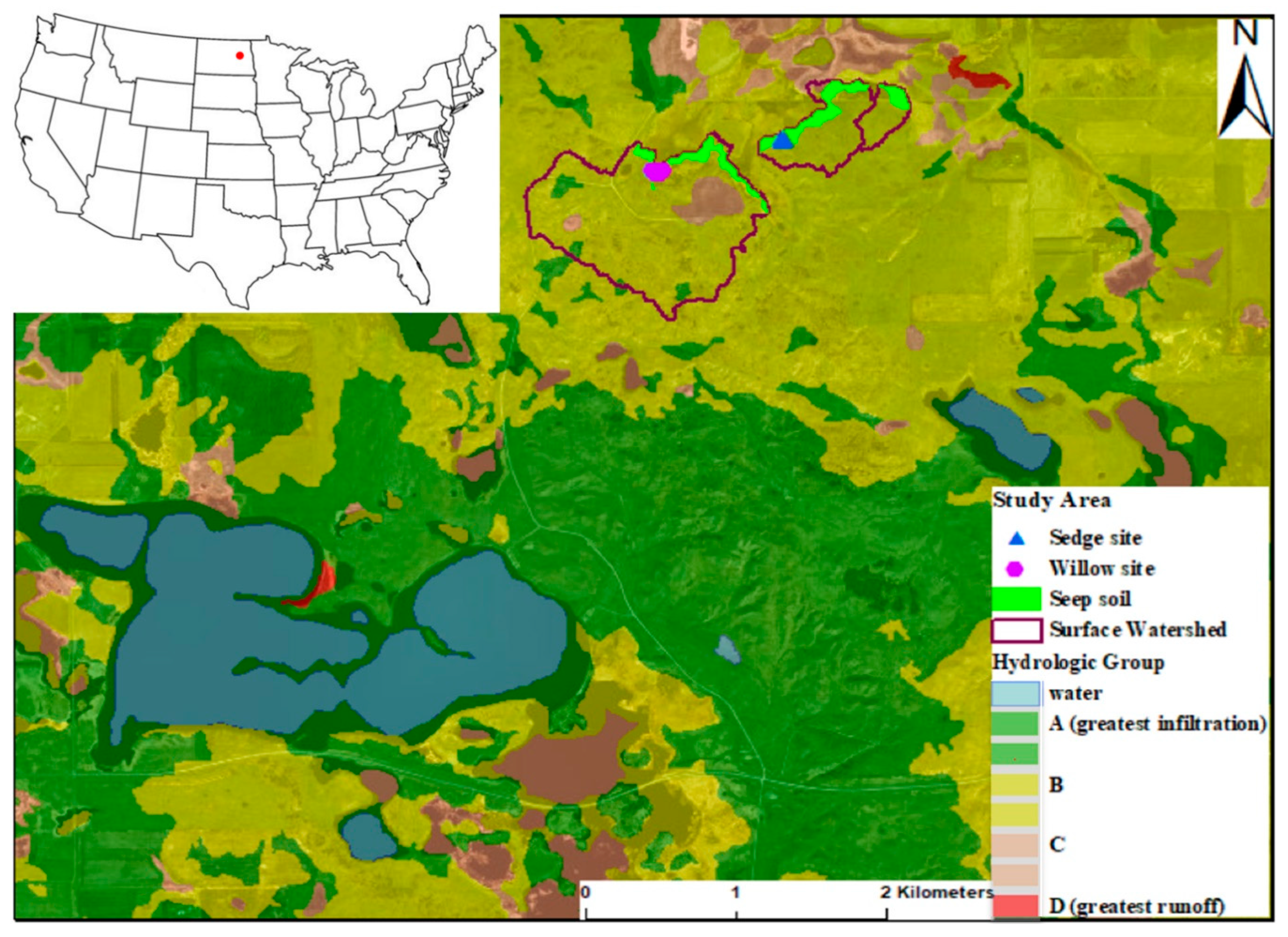
This research focuses on two sites about 800 m apart within a single, large seepage zone in central North Dakota. One site is shrub and tree covered and referred to as the Willow site. The other site is characterized by nearly all fibrous-rooted herbaceous plant cover and referred to as the Sedge site. The large seepage zone fen, extending roughly 2000 m and covering 2000 m2, is located within the North Dakota National Guard—Camp Grafton South (CGS) facility, Eddy County, North Dakota (47°43’42” N, 98°39’41” W) (Figure 1). CGS covers 31 km2, but the portion of interest extends over about 2.5 km2. CGS is underlain by stratified glacial deposits, till and outwash, which overlie the Cretaceous Pierre Formation [21]. The hydrogeology of CGS, geomorphology, stratigraphy, and water quality of CGS was recorded in details [21]. Based on hydrogeological criteria developed by Winter et al., [2] this wetland is classified as a fen. Fens with high species diversity usually have moderate pH; the pH of this fen ranges from 7.23 to 7.67 [22,23].
The fen and study sites were selected because of their diverse and well-known plant community, perhaps more diverse than any wetland in North Dakota [22]. Plant communities common at this location are the cattail marsh, herbaceous meadow, and wooded wet meadow. Certain species present at this wetland are among those proposed for conservation priority in North Dakota. Species are ranked in levels; Level I, Level II, or Level III to prioritize conservation efforts. Six species found at the study site are on the proposed list for conservation. Cypripedium candidum (White Lady’s-slipper) is a Level I species, Cypripedium parviflorum (Small Yellow Lady’s-slipper Orchid) and Carex sterilis (Sterile Sedge) are Level II species, and Parnassia palustris (Small-flowered Grass-of-Parnassus), Rhynchospora capillacea (Hair Beakrush) and Utricularia intermedia (Flat-leaved Bladderwort) are Level III species [24]. The presence of these species within the study area makes this site a priority for conservation in North Dakota. Hydrological alteration of the wetland would cause degradation of the vegetative communities within these ecosystems [22]. Installation and monitoring using the conventional method was restricted to small areas of the fen and carried out entirely by hand, so as to minimize disturbance.
The location is currently used by the National Guard for training and needs to be protected against any contamination, environmental degradation and extinction of the diverse plant community. The primary land use contaminant in Camp Grafton South is munitions, explosives, and cattle grazing. The location is leased for grazing during spring and fall, which raises the possibility of contamination from livestock waste [25].
The seep soils at the study site are mapped as hydrologic group B (Figure 1) [26]. Group B has moderate low runoff potential when wet, high porosity and permeability, and unimpeded water transmission, consisting of 10–20% clay and 50–90% silty-sand. The Willow and Sedge sites form a groundwater discharge zone (seepage area) for the Cherry Lake Aquifer [21].
2. Methods
2.1. Field Measurement and Mapping
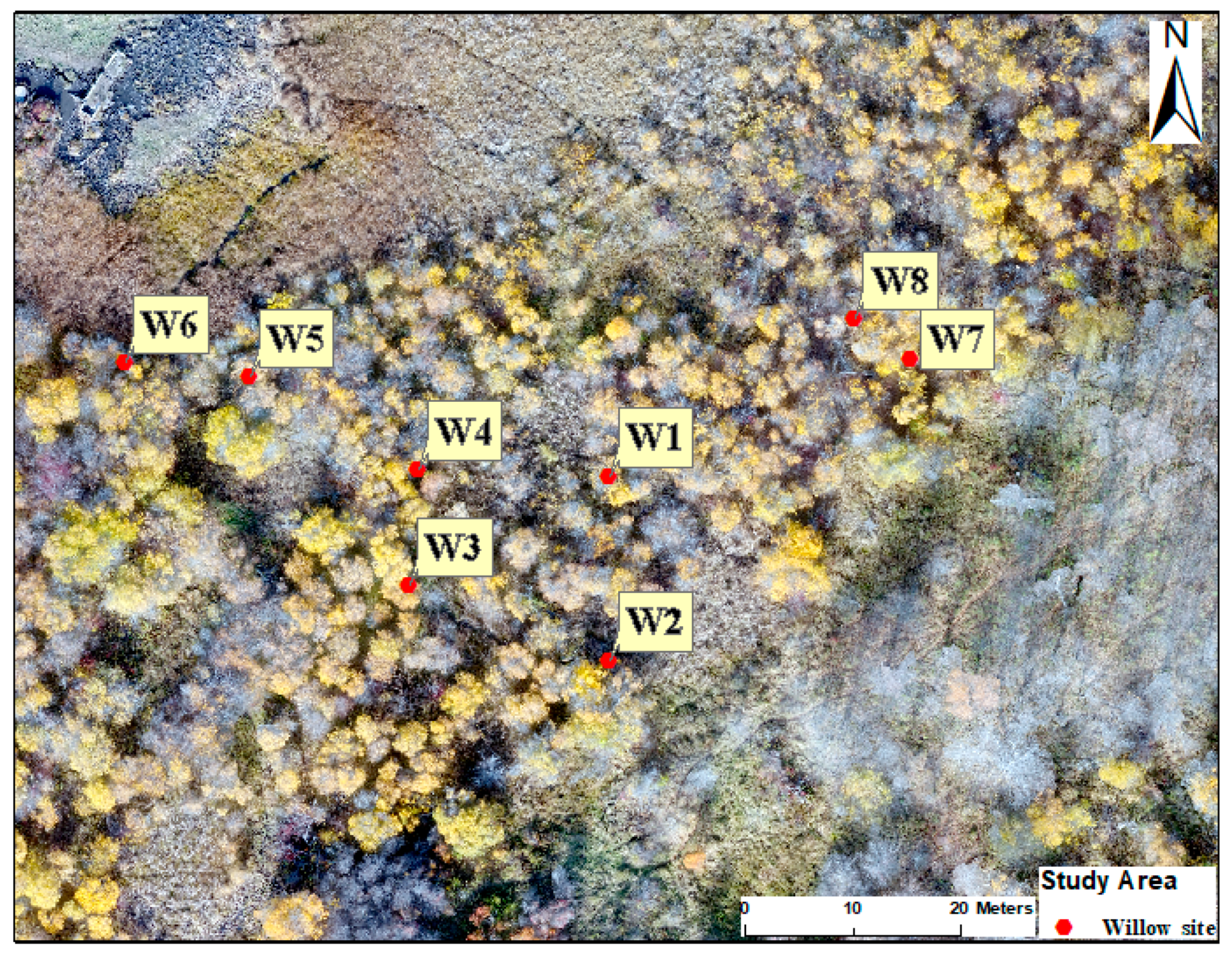
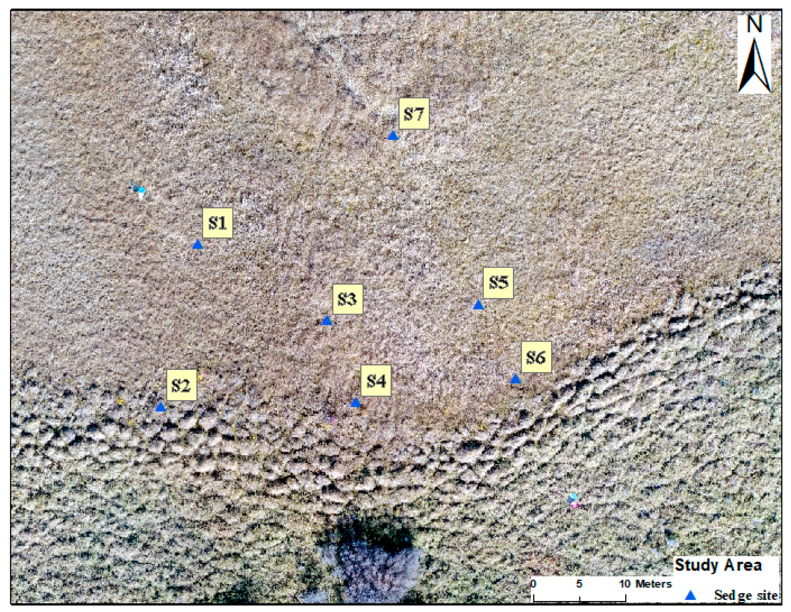
An on-the-ground approach was used to capture thermal images. The coldest temperature reading for each of the images was plotted against the results determined from the conventional method of using field instrumentation and Darcy’s law to measure hydraulic gradient and flux. Onset® HOBO pendant temperature data loggers (Onset Computer Corporation, Bourne, MA, USA) were installed to measure surface water temperatures at all the points in the study area. Eight points in the Willow site and seven points in the sedge site were closely distributed within the sites to provide an overview of the subsurface processes (Figure 2 and Figure 3).
2.2. Soil Classification
The seep soil (Figure 1) at the study site is a complex of several soil series and their proportions: Vallers—35%, Hamerly—25%, Wyndmere—20%, Arveson—14%, Balaton—3% and Seeleyville—3%. The seep soil is classified as having 2–6% slopes and is poorly drained. It has a clay range of 14–26%, sand range of 38–70%, organic matter of 5–8% at the depth <20 cm, and saturated hydraulic conductivity K range of 2 × 10⁻⁵–8 × 10⁻⁶ [27].
2.3. Conventional Method
2.3.1. Hydraulic Gradient
Estimating groundwater seepage and direction using Darcy’s flow is the conventional method, which may be accomplished by installing tensiometers to measure pressure head (usually negative), elevation head and total head. A tensiometer is a small (2 cm) diameter closed tube with a porous tip (ceramic cup) [28]. The tensiometer is filled with water, sealed with the septum stopper, and the end with the ceramic cup pushed into the soil. As water moves from the tube to the soil through the porous ceramic cup, the tension inside the tube reaches equilibrium with the soil water. A portable tension transducer and gauge (Soilmoisture Equipment Corporation, Santa Barbara, CA, USA) is then used to measure the tension (negative pressure) created inside the tensiometer. The measured differences in hydraulic head within the flow system are used to determine the groundwater flow direction. In many instances, the tensiometer cup was seated below the water table, thereby creating small positive pressure heads which were analogous to piezometers.
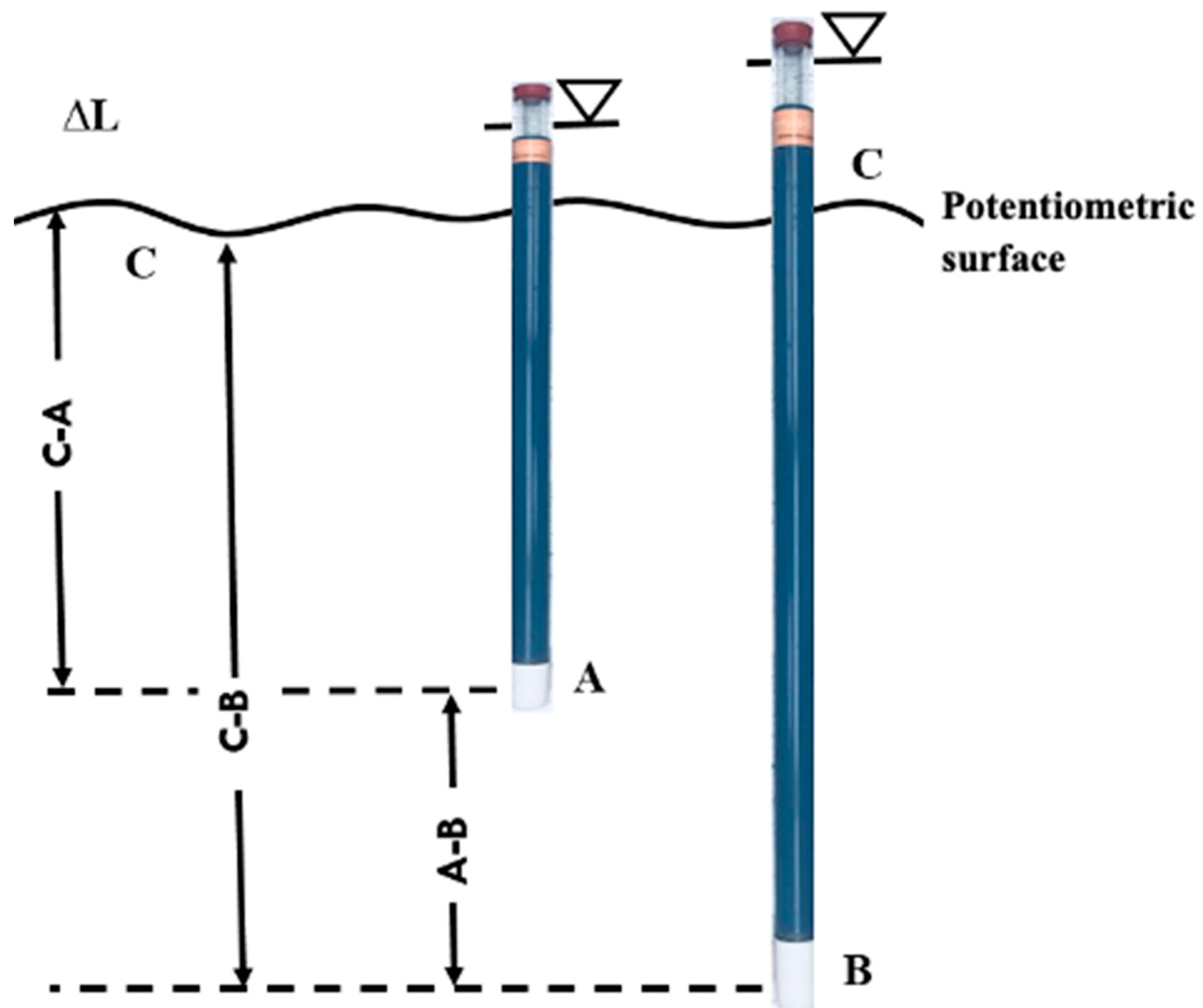
Darcy’s law was used to estimate the groundwater flow direction and seepage rate, based on measured hydraulic gradients and hydraulic conductivity. Tensiometer pairs were installed at points in the fen to solve for the vertical gradient; three hydraulic gradients between points A–B, B–C, and A–C were measured (Figure 4).
Hydraulic gradient determines the flow direction and was characterized using pairs of tensiometers seated at different depths to estimate hydraulic heads based on an assumed datum on-site or mean sea level. For this study, downward flow, i.e., decreasing hydraulic heads with greater depth, the hydraulic gradient is assumed positive (+) and the flow is downward. Similarly, where the gradient is negative (−), head increases with depth, then the flow is upward.
2.3.2. Hydraulic Conductivity
Hydraulic conductivity, K describes the rate at which water can move through a permeable medium under unit hydraulic gradient. Although many characteristics affect K, such as particle size distribution, roughness, tortuosity, porosity, bulk density, shape, and degree of interconnection of water-conducting pores, we estimated hydraulic conductivity empirically by using the Bouwer and Rice slug test method [29]. This in situ field test method is based on the principle that the rate at which the soil transmits water from a well screen and casing is related to the saturated soil K:
where K is hydraulic conductivity (L/t);
rc is the radius of the well casing (L);
R is the radius of the well (including gravel envelope) (L);
Re is the radial distance over which head is dissipated (L);
Le is the length of the screen (L);
t is the time since H = H0 (t);
H0 is the drawdown at time t = 0 (L);
H is the drawdown at time t = t (L), with L representing length and t representing time for units.
This test estimate application was achieved in the field by installing a partially penetrating hydrometer in the subsurface.
2.3.3. Darcy Flux
The vertical Darcy flux at the monitoring points within the two sites was calculated using the result from the hydraulic gradient and estimated saturated hydraulic conductivity. For vertical flux, q is expressed in terms of the hydraulic head applied through a porous medium.
where q is the vertical flux; K is the hydraulic conductivity; dh is change in head between each pair of tensiometer; and L is the vertical distance between the adjacent tensiometer cups. The hydraulic gradient and the hydraulic conductivity were substituted into Darcy’s law to estimate the vertical flux at each monitoring point in the field. Vertical flux q was then used to correlate with temperatures estimated from thermal images.
2.4. Thermal Imaging
Thermal images were captured using a FLIR Systems C2 camera (Wilsonville, OR, USA). The FLIR C2 measured surface temperature using a 320 × 240 focal plane arrays with a spectral range of 7.5–14 µm. The camera sensor pixels are heated by the incoming infrared radiation, thereby changing the pixel resistance. The pixel resistance is measured and calibrated to a temperature value, and the temperature raster is presented as an image. Infrared cameras have several thousand gridded measurement sensors, analogous to a thermometer measuring temperature at every spot. In a 320 × 240 focal plane array, a 76,800-infrared pixel image with a temperature value at each pixel was achieved. It is a full-featured, pocket-sized thermal camera. The captured thermal images, superimposed with visible light features, was used to identify the hot and cold spots in the field.
The FLIR C2 was used at ground-based to capture thermal images at every monitoring point (Figure 2 and Figure 3) for both sites and the temperature value plotted against the hydraulic gradient for each point. Images were captured before sunrise to eliminate all interference from reflection and absorption of heat by materials on the ground surface of the fen.
Thermal Aerial Imagery
The thermal aerial imagery of Sedge site was captured using an unmanned aerial vehicle (UAV) on 13 October 2017 by Dr. Joao Paulo Flores of North Dakota State University’s Carrington Research Station. A hexacopter (DJI S900) fitted with a thermal camera (ICI 8640P Series) was flown on approval to collect thermal imagery from the research site. Thermal imagery was collected over only the Sedge site and not the Willow site because of the tree cover and thick vegetation, which prevented the aerial view of the site’s ground surface. In addition to the DJI S900 hexacopter, missions were flown with a DJI Phantom 4 Pro quadcopter, which was equipped with a 20.1 mega pixel resolution RGB camera. Prior to each flight, three targets placed in a broad triangle were set out at both research sites in order to validate georeferencing data gathered by the instruments. The thermal aerial imagery was used to visualize the temperature trend on the site and, map cooler areas, which may indicate groundwater seepage. Thermal imagery was also used to map distinct boundaries of vegetation, water boundaries, and the local break-in-slope.
3. Results
3.1. Conventional Method
3.1.1. Soil Classification of the Fen
The seep soils at the study site are mapped as hydrologic group B (Figure 1) [26]. Group B has moderate low runoff potential when wet, high porosity and permeability, and unimpeded water transmission with 10–20% clay, 50–90% silty-sand. All the monitoring points at the Willow site were on the seep soil, the Sedge site has all of its points on the seep soil except for monitoring points S2, S4, and S6.
3.1.2. Hydraulic Gradient
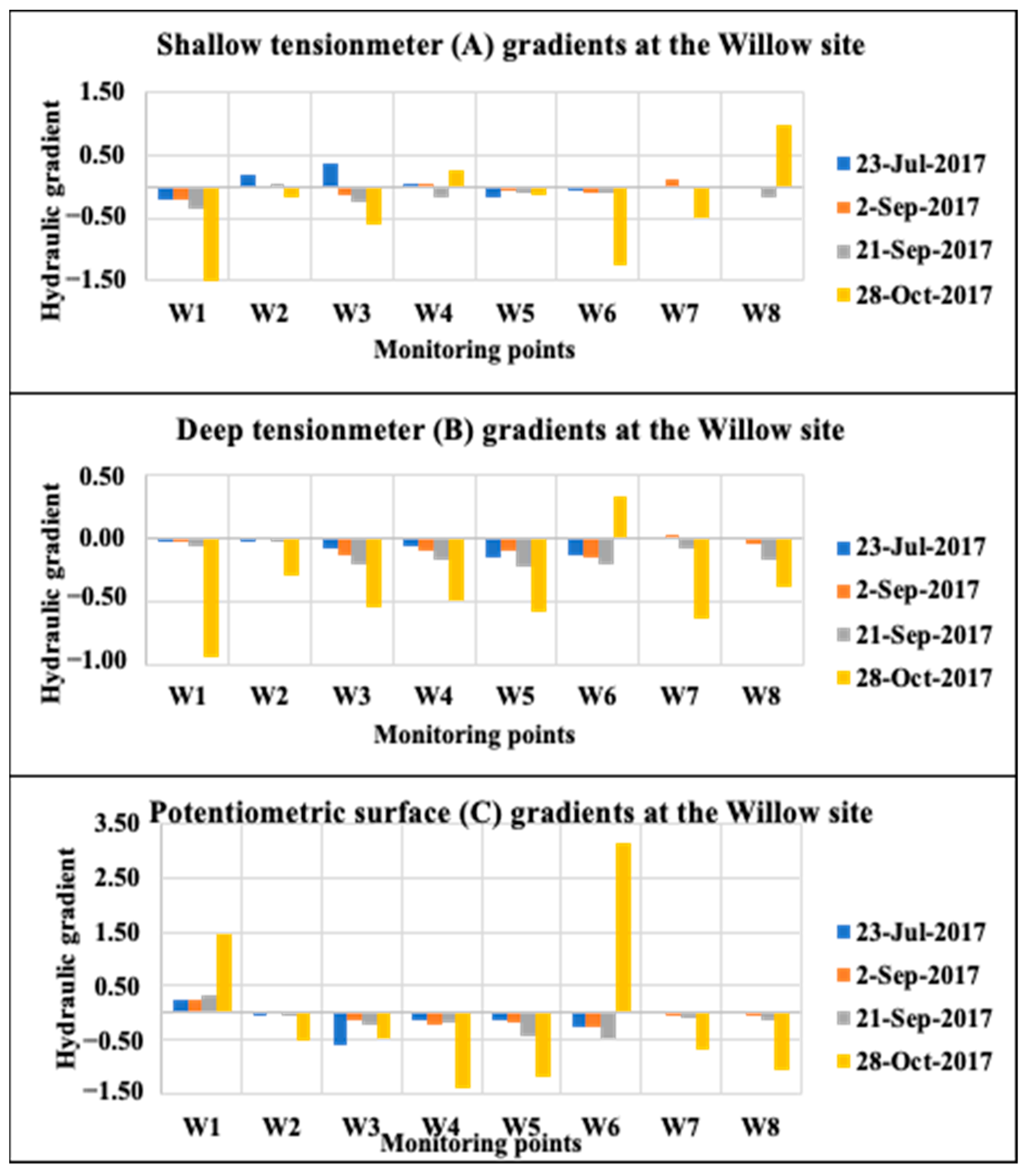
Monitoring points at both the Willow (Figure 2) and Sedge (Figure 3) sites revealed variable gradients (Figure 5). The plot of the gradient at the shallow tensiometer for most points in the Willow fen showed upward gradient on most dates (Figure 5A). For the deep tensiometer, W7 and W6 showed an upward gradient on 2 September and 28 October 2017, respectively (Figure 5B). Gradients at the potentiometric surface (Figure 5C) for most monitoring points revealed upward flow except for W1 on all dates and W6 on 28 October 2017.
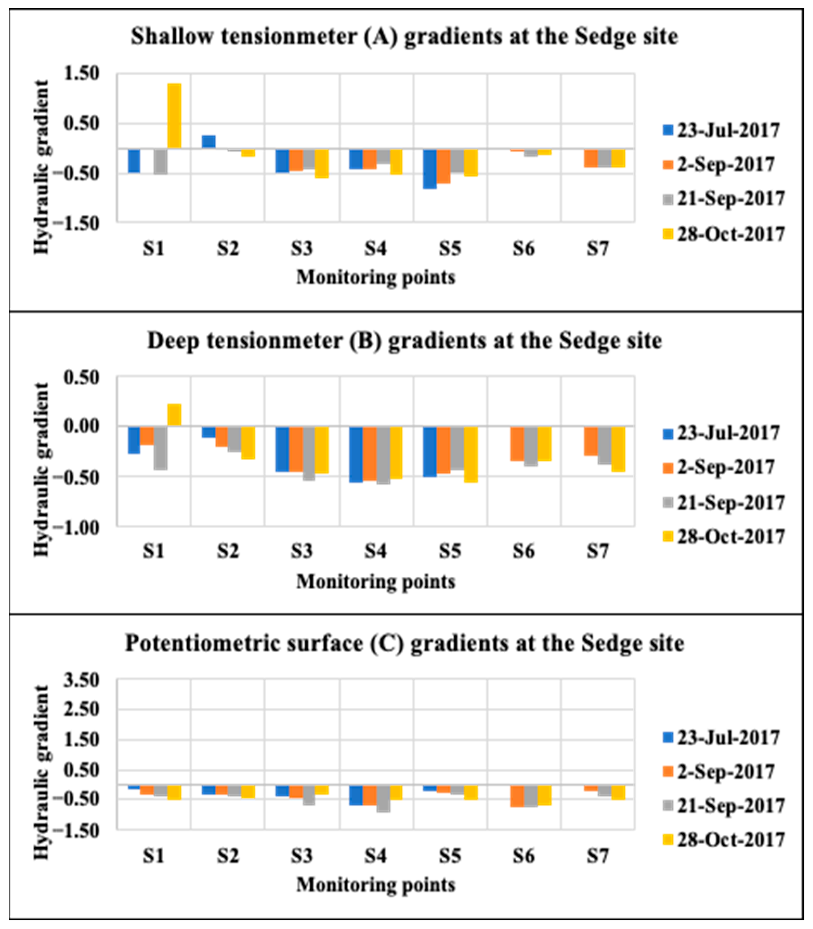
The plot of the shallow tensiometer gradients for all the monitoring points at the Sedge fen showed strong upward gradient except for S1 on 28 October 2017 and S2 on 23 July 2017 (Figure 6A). Deep tensiometer gradients for all the monitoring wells are upwards except for S1 on 28 October 2017 (Figure 6B). The potentiometric surface gradients for all the monitoring points at the Sedge site are all upward flow (Figure 6C). The potentiometric surface hydraulic gradient defines the seepage interaction at the near-surface between the potentiometric surface and the shallow tensiometer. The shallow hydraulic gradient defines the hydraulic gradient between the shallow and deep tensiometer, whereas the deep hydraulic gradient is between the potentiometric surface and the deep tensiometer.
3.1.3. Hydraulic Conductivity
The estimated average hydraulic conductivity for the Willow site is somewhat larger than the Sedge site. The hydraulic conductivity, K, for the Willow site ranged from 6 × 10⁻⁵ to 2 × 10⁻⁴ m/s: and Sedge site: 6 × 10⁻⁶ to 1 × 10⁻⁴ m/s (Table 1), which falls within values typical for fen sediments [30].
3.1.4. Darcy’s Flux
The hydraulic gradient measured on 28 October 2017 and hydraulic conductivity were substituted into Darcy’s law to estimate the groundwater flux for each monitoring point. The positive and negative sign before the flux shows the direction of flow; downward flow if positive (+) sign, and upward flow if negative (−) sign. The flux calculated for the Willow site ranged from 1.4 × 10⁻⁵ to 2.7 × 10⁻⁴ m/s (Table 2) and that of the Sedge site ranged from 2.2 × 10⁻⁶ to 6.3 × 10⁻⁵ m/s (Table 3).
3.2. Thermal Imaging
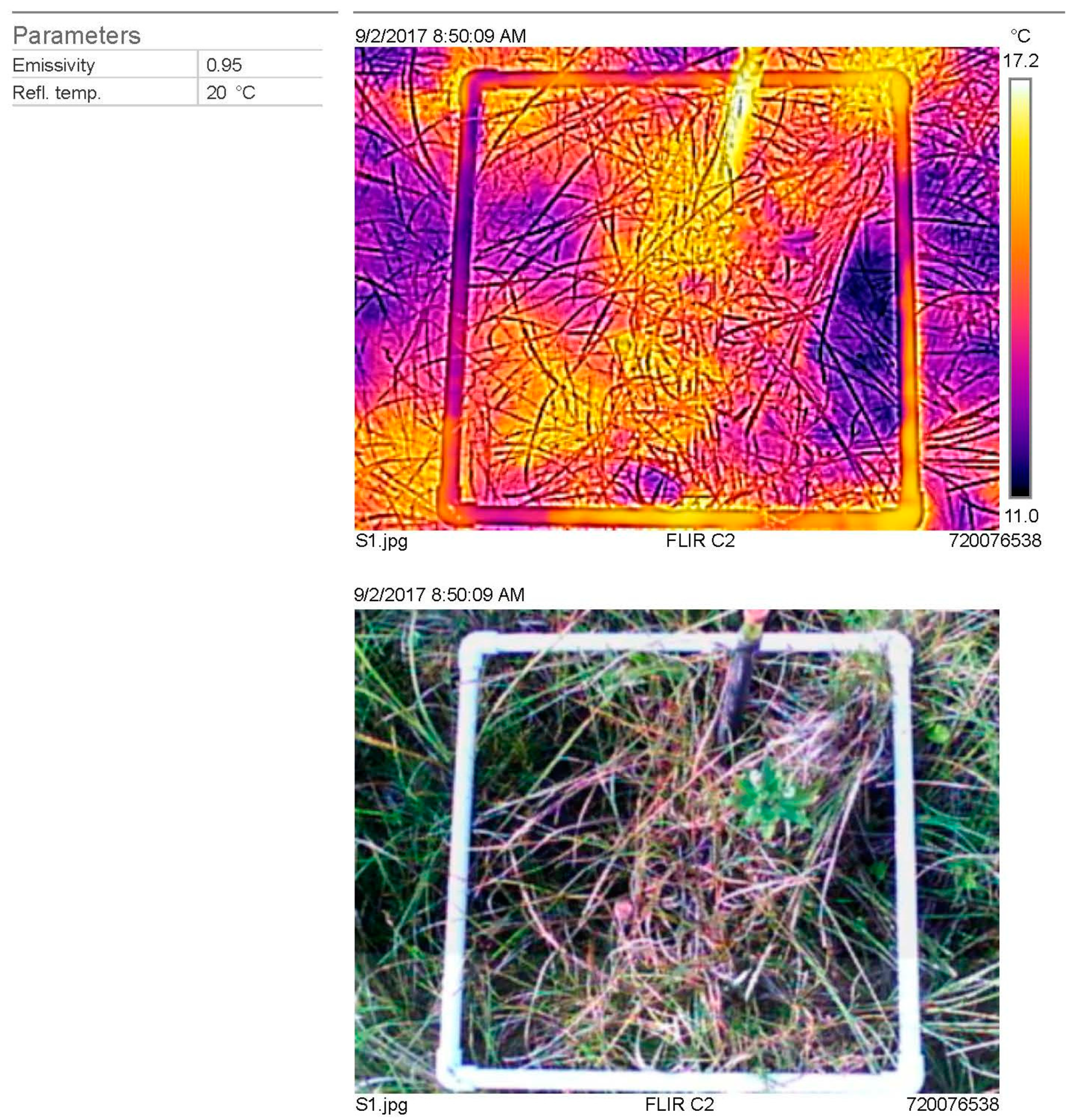
Thermal images were captured at the same monitoring points where hydraulic gradient and conductivity were measured. The temperature values for the both sites were extracted from the thermal image for each date of data capture (Table 4 and Table 5). The coldest temperature was used because groundwater temperature is expected to be cooler than the surface temperature at the time when the thermal images were captured (1 July, 23 July, 2 September, 21 September). The warmest temperature was used for 2 December 2017 because groundwater temperature is warmer than the surface water during the winter season. Figure 7 shows one of the thermal images captured using the FLIR C2 camera, with temperatures ranging from 17.2 to 11.0 °C and a digital visible light image of the surface.
3.3. Thermistor Data
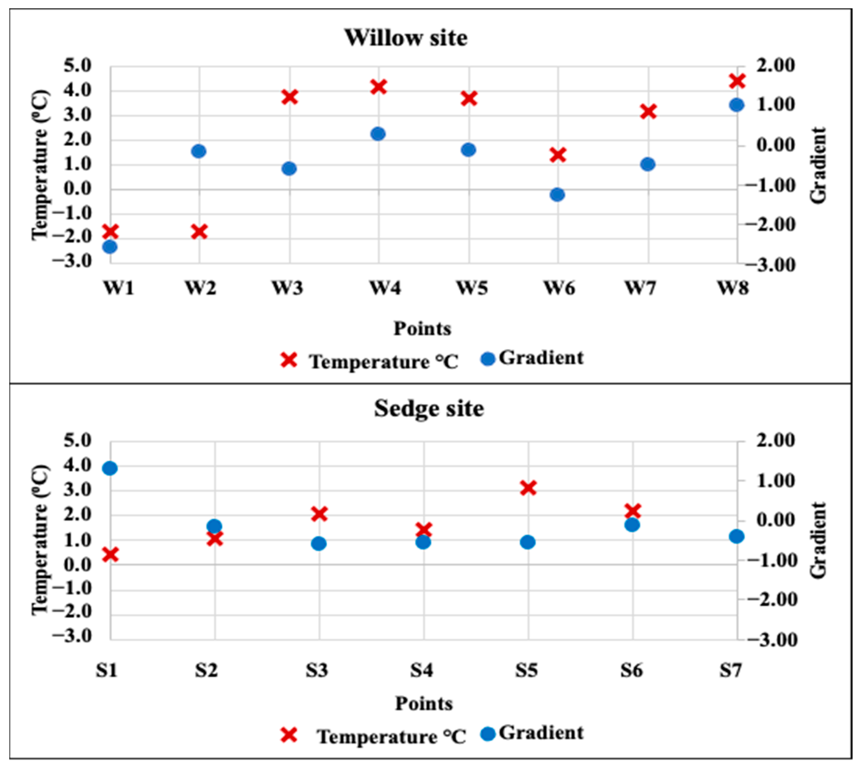
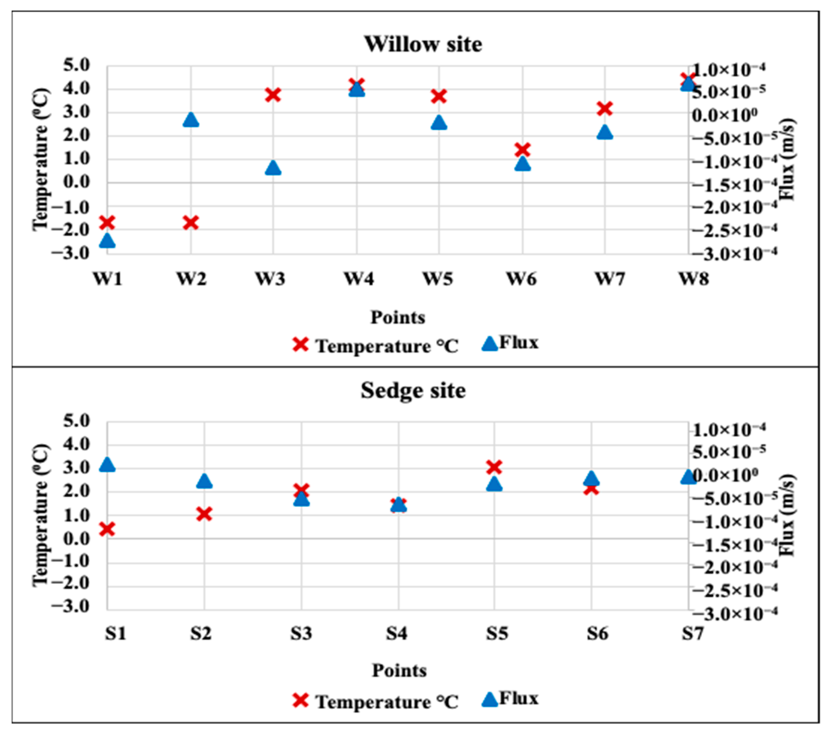
Thermistor temperature readings were plotted for 9 a.m. at the Willow site and 10 a.m. at the Sedge site on 28 October 2017, which correspond to the time that the hydraulic gradient was measured on-site. With the data collected on 28 October 2017, graphs of temperature versus hydraulic gradient (Figure 8) and temperature versus flux (Figure 9) were plotted for both sites.
3.4. UAV Thermal Imagery
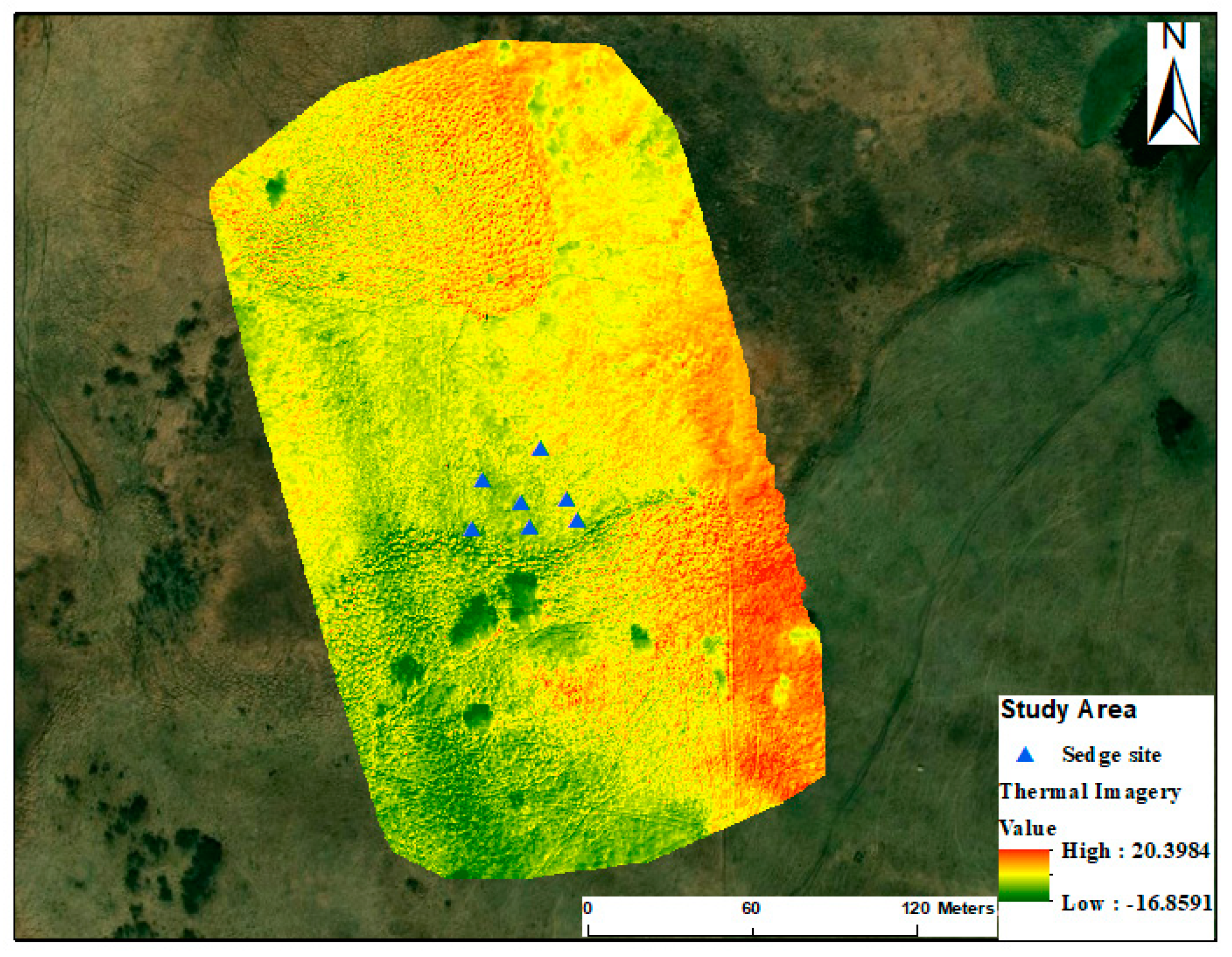
The northern portion of the aerial thermal imagery at the Sedge site (Figure 10) shows a distinctive boundary of the mounds that occur at the site, the green areas show seepage, shrubs, and trees, and the break-in-slope is evident just to the south of the monitoring points. The green areas are also possibly cold spots indicating upwelling of colder groundwater to the surface. The groundwater seepage areas seen on the thermal imagery supports seep soil structure (Figure 10), which permits seepage of groundwater to the surface. For every temperature value on the UAV thermal imagery within and below the average groundwater temperature of 4 °C [31] at this site, indicates groundwater seepage.
3.5. Temperature Profile
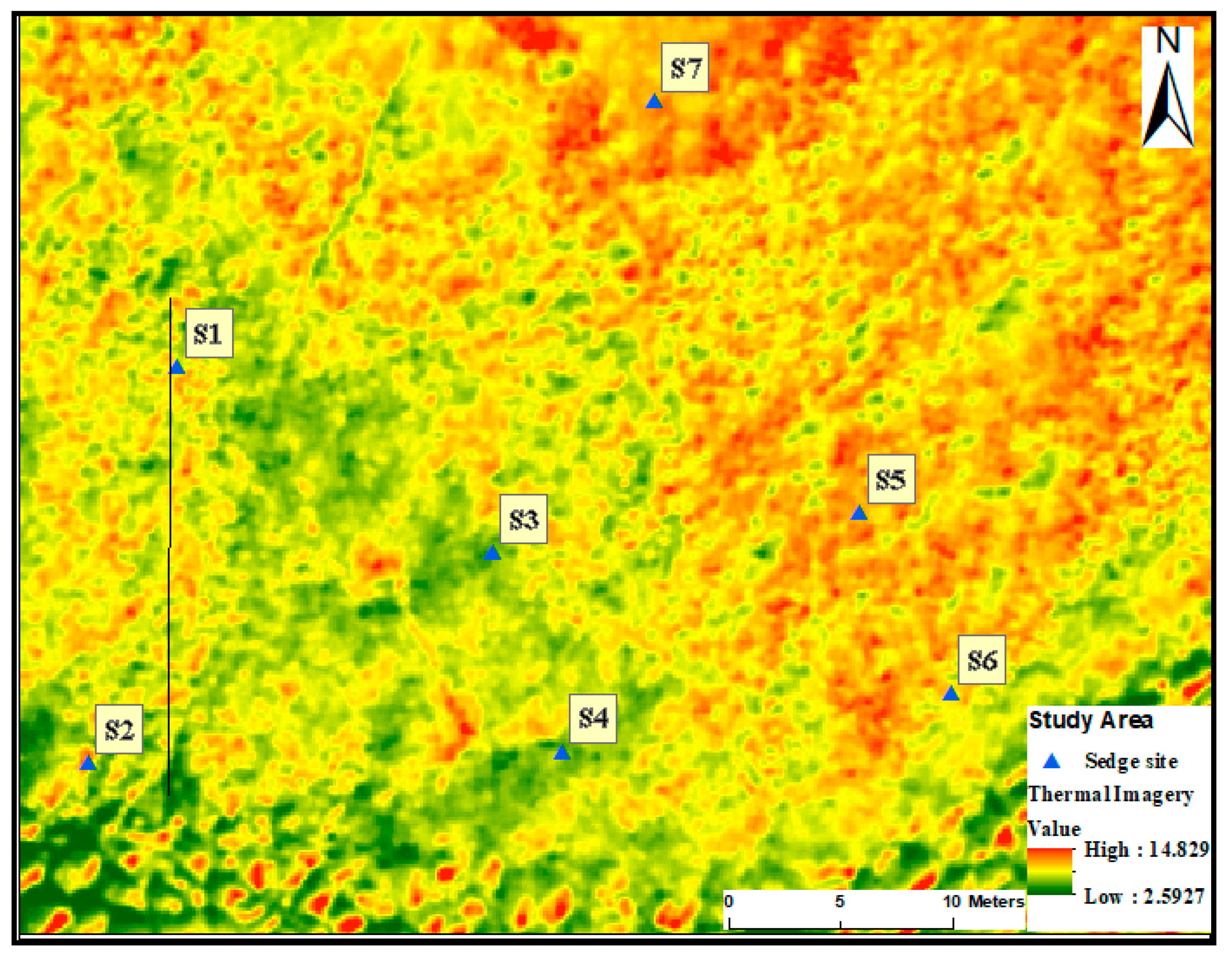
On 21 September 2017, a temperature image profile was captured for the Willow site and Sedge site using the FLIR C2. The interpolated temperature profile line on the aerial thermal imagery at the Sedge site (Figure 11) in a south–north direction was compared with a temperature profile from the FLIR C2 (Figure 12B).
The interpolated temperature profile of the thermal imagery (Figure 12C) showed a similar temperature trend with the temperature profile at the Sedge site, although the FLIR C2 and UAV images were captured on different dates (21 September and 13 October, respectively). The result of both profiles shows that temperature increased downslope, which likely results from progressive warming of the discharged groundwater.
4. Discussion
4.1. Darcy’s Flow
Monitoring points at the Willow site revealed variable gradients (Figure 5 and Figure 8), perhaps related to greater transpiration from surrounding vegetation as described in the wetland plant root classification in Lai et al., 2011. Trees and shrubs at this location have deeper and larger roots, which may explain the more heterogeneous and stronger water uptake, causing greater transpiration. In contrast, herbaceous vegetation has finer, denser, and more shallow root systems that may lead to lower and more consistent rates of transpiration. W1 is installed within a Salix spp. (willow) thicket, which may be drawing water from the surface to its roots to support root activity. All the gradients measured at the Sedge site (Figure 6) showed upward flow, except for the shallow (Figure 6A) and deep (Figure 6B) hydraulic gradient for monitoring point S1 in October. The reason for this behavior can be defined more if the stratigraphy is investigated in detail or might be attributed to disturbance to the soil profile. Monitoring points S4 and S6, located about 2 m from the break-in-slope at the Sedge site, showed more groundwater seepage, based on the result of the hydraulic gradient (Figure 6) than points S3 and S5, which were about 10 m farther from the break-in-slope. A monitoring point in between S2 and S1 would reveal more about the hydraulic gradient trend, as shown between S3 and S5. At monitoring point S7, the seepage rate was between −0.39 and −0.40 m/s and about 60 percent less than the seepage in point S5, which ranged between −0.69 and −0.50 m/s. These observations suggest that groundwater seepage occurs more at the break-in-slope than it occurs northward within the wetland. The conventional method of characterizing groundwater seepage stands to quantify the rate of flux and the vertical direction of flow, but it is equipment intrusive and labor intensive, and disturbs the soil profile, which results from entrance and installation of equipment in the field.
All the monitoring points at the Willow site and S1, S3, S5, and S7 at the sedge were on the seep soil. This information confirms that the soil stratigraphy likely permits the groundwater to seep to the surface. The Willow and Sedge sites form a groundwater discharge zone (seepage area) for the Cherry Lake Aquifer.
4.2. Thermal Imaging
Mapping cold spots in summer and warm spots in winter suggested points and zones where groundwater seepage occurs at this location. Based on the coldest observed temperature from the FLIR C2 at the Sedge site (Table 5), monitoring point S2 showed a lower temperature reading than point S1, suggesting more groundwater seepage at point S2 than at point S1. Points S3 and S4 showed similar behavior as point S1 and S2, except on 23 July 2017.
In general, groundwater temperature is expected to be higher than surface water temperature during winter [31]. Point S4 had greater temperature than point S3, suggesting groundwater seepage occurring at point S4 during winter (2 December 2017). The thermal images acquired in this research add to the many studies that indicate temperature can be used to trace groundwater seepage (e.g., [1,5,12,13,14,15,16,17].
Identifying groundwater seepage depends strongly on the temperature difference between surface water and groundwater. Cold spots in summer indicated upwelling of relatively colder groundwater to the surface to disrupt the surface water temperature, warm spots indicated upwelling of relatively warmer groundwater from the subsurface to the surface to heat the cold and frozen surface water temperature in winter. Thermal imaging at the Willow site did not show a similar trend with the hydraulic gradient, suggesting that shade from vegetation can affect temperature readings during spring to late summer season. This is unlikely because most of the leaves had fallen by the time the measurements were made. Alternatively, heterogeneous soils and shallow soil stratigraphy may influence gradients. For example, if a much less pervious layer lies between the surface and the shallow underlying aquifer, a strong vertical gradient may be indicated with the piezometric measurements, but the flow and subsequent discharge move laterally to a different point. Thus, the thermal signal at the surface for a strong vertical gradient may be absent.
Aerial thermal imagery (Figure 10) showed wetland surface features: a distinct vegetation boundary, break-in-slope above the fen, and the wetland boundary. Due to poor resolution, however, aerial imagery lacks the details of the temperature change of the environment as would the on-the-ground thermal images (Figure 7). Aerial thermal imagery is helpful in certain conditions, by providing less environmental noise, easier calibration, and more convenient image processing. Aerial thermal imagery may not be used to characterize or quantify the groundwater seepage in areas with thick and dense vegetation, such as the Willow site because of shadowing from surrounding vegetation, although good results may be possible during periods of senescence.
The temperature profile from the thermal imagery (Figure 12C) of the Sedge site showed a similar temperature trend with the temperature profile acquired using the FLIR C2 (Figure 12B). The temperature profile acquired on-the-ground eliminates possible environmental noise (topographic features, such as the sedge mounds and structural obstructions), which the thermal aerial imagery captured. Applying a moving average of period 10 (Figure 12C) dampened the noise during processing of the temperature profile trend.
Snapshot-in-time and surface-skin nature of thermal imaging data limited groundwater seepage detection at the research location. However, under the right set of conditions on-the-ground thermal imaging and aerial thermal imagery may provide detail on groundwater seepage dynamics [3] similar to data collected in situ from field equipment (conventional method) for a fraction of the effort.
Based on the analysis of our results, identification of groundwater seepage using thermal imaging trends correlate qualitatively with the conventional method. On-the-ground thermal imagery data collection is therefore quick, less labor intensive, provides point-in-time evaluation, although influenced by environmental and physical factors, and measurements are limited to the surface (skin) temperature of water features.
Thus, the application of thermal imaging to map groundwater seepage requires both remote and direct temperature measurement and additional data on soil stratigraphy to fully capture the seepage zone at this site.
5. Conclusions and Recommendation
Using heat as a groundwater tracer is a valuable and easily applied tool when the temperatures of the surface water contrasts strongly with the temperature of the groundwater. For example, localized groundwater discharge can be detected and quantified in wetland ecology studies. This study aimed at using temperature differential between the surface water and the groundwater in midsummer and midwinter to characterize seepage. The information obtained from this research can be used to map areas and zones in the wetland that are connected with the groundwater.
Thermal imaging is quick, less-labor intensive, and provides point-in-time evaluation. Thermal imaging is therefore qualitative, indicating broad zones of groundwater seepage and subjectively characterizing the flow rate and direction, but cannot be used to quantify groundwater seepage at this fen. The conventional method is quantitative and can be used to characterize groundwater seepage at this fen. Thermal imaging can be used if the aim of the study is to simply indicate areas of groundwater seepage at the surface. In the case of using thermal imaging to indicate groundwater seepage, thermal imaging should be captured at night to eliminate all interference from reflection and absorption of heat by materials on the ground surface of the fen.
Soil heterogeneity is also a major factor influencing groundwater seepage. Fined-grained layers of soil near surface can prevent seepage from reaching the surface because of the hydraulic conductivity of fined-grained soil are low compared to seep soil. Groundwater seepage at Willow and Sedge site can only be measured and quantified by using conventional methods. Understanding and defining the soil layer properties accurately is significant in characterizing groundwater seepage, especially when using temperature as a groundwater seepage tracer because soil permeability can alter the flow rate of groundwater to the surface. Further research on the layer properties can be obtained by studying the soil stratigraphy within the fen.
Thermal imaging can assist water resource and environmental managers in mapping and characterizing zones of groundwater seepage to identify areas susceptible to groundwater–surface water quality influence.
Author Contributions
Conceptualization, O.O. and P.J.G.; methodology, O.O. and P.J.G.; validation and formal analysis, O.O.; investigation, O.O.; resources and data curation, O.O. and P.J.G.; writing—original draft preparation, O.O.; writing—review and editing, O.O. and P.J.G.; visualization, O.O. and P.J.G.; supervision, P.J.G.; project administration, O.O. and P.J.G.; funding acquisition, O.O. All authors have read and agreed to the published version of the manuscript.
Funding
Funding for this research was provided by the Harold Hamm School of Geology and Geological Engineering, College of Engineering and Mines, University of North Dakota, and the Ivanhoe Foundation.
Institutional Review Board Statement
Not applicable.
Informed Consent Statement
Not applicable.
Data Availability Statement
The data presented in this study are within the article.
Acknowledgments
Authors wish to acknowledge Kent Belland and the North Dakota National Guard for permission to access the study site, and thank Joao Paulo Flores, North Dakota State University, Carrington Research Station, for the UAS data acquisition and processing.
Conflicts of Interest
The authors declare no conflict of interest. The Funders has no role in the design of the study; in the collection, analyses, or interpretation of data; in the writing of the manuscript, or in the decision to publish the results.
References
- Banks, W.S.L.; Paylor, R.L.; Hughes, B.W. TIR for groundwater discharge. Groundwater 1996. [Google Scholar] [CrossRef]
- Winter, T.C.; Judson WHarvey Franke, O.L.; Alley, W.M. Ground Water and Surface Water: A Single Resource; DIANE Publishing Inc.: Darby, PA, USA, 1999. [Google Scholar] [CrossRef]
- Hare, D.K.; Briggs, M.A.; Rosenberry, D.O.; Boutt, D.F.; Lane, J.W. A comparison of thermal infrared to fiber-optic distributed temperature sensing for evaluation of groundwater discharge to surface water. J. Hydrol. 2015, 530, 153–166. [Google Scholar] [CrossRef] [Green Version]
- Brunner, P.; Therrien, R.; Renard, P.; Simmons, C.T.; Franssen, H.J.H. Advances in understanding river-groundwater interactions. Rev. Geophys. 2017, 55, 818–854. [Google Scholar] [CrossRef]
- Deitchman, R.S.; Loheide, S.P. Ground-based thermal imaging of groundwater flow processes at the seepage face. Geophys. Res. Lett. 2009, 36, 1–6. [Google Scholar] [CrossRef]
- Danielescu, S.; MacQuarrie, K.T.B.; Faux, R.N. The integration of thermal infrared imaging, discharge measurements and numerical simulation to quantify the relative contributions of freshwater inflows to small estuaries in Atlantic Canada. Hydrol. Process. 2009, 2274, 2267–2274. [Google Scholar] [CrossRef]
- USEPA United States Environmental Protection Agency. Wetland Classification and Types. 2016. Available online: https://www.epa.gov/wetlands/wetlands-classification-and-types#fens (accessed on 1 December 2016).
- Winter, T.C.; Rosenberry, D.O.; Buso, D.C.; Merk, D.A. Water source to four U.S. wetlands: Implications for wetland management. Wetlands 2001, 21, 462–473. [Google Scholar] [CrossRef]
- Lai, W.L.; Wang, S.Q.; Peng, C.L.; Chen, Z.H. Root features related to plant growth and nutrient removal of 35 wetland plants. Water Res. 2011, 45, 3941–3950. [Google Scholar] [CrossRef] [PubMed]
- Dahm, C.N.; Grimm, N.B.; Marmonier, P.; Valett, H.M.; Vervier, P. Nutrient dynamics at the interface between surface waters and groundwaters. Freshwater Biol. 1998, 40, 427–451. [Google Scholar] [CrossRef]
- Valett, A.H.M.; Dahm, C.N.; Campana, M.E.; Morrice, J.A.; Baker, M.A.; Fellows, C.S. Hydrologic influences on groundwater-surface water ecotones: Heterogeneity in nutrient composition and retention. J. N. Am. Benthol. Soc. 1997, 16, 239–247. [Google Scholar] [CrossRef]
- Loheide, S.P.; Gorelick, S.M. Quantifying stream-aquifer interactions through the analysis of remotely sensed thermographic profiles and in situ temperature histories. Environ. Sci. Technol. 2006, 40, 3336–3341. [Google Scholar] [CrossRef] [PubMed]
- Schuetz, T.; Weiler, M. Quantification of localized groundwater inflow into streams using ground-based infrared thermography. Geophys. Res. Lett. 2011, 38, 1–5. [Google Scholar] [CrossRef]
- Anderson, M.P. Heat as a ground water tracer. Ground Water 2005, 43, 951–968. [Google Scholar] [CrossRef] [PubMed]
- Bravo, H.R.; Jiang, F.; Hunt, R.J. Using groundwater temperature data to constrain parameter estimation in a groundwater flow model of a wetland system. Water Resour. Res. 2002, 38, 28-1–28-14. [Google Scholar] [CrossRef]
- Lowry, C.S.; Walker, J.F.; Hunt, R.J.; Anderson, M.P. Identifying spatial variability of groundwater discharge in a wetland stream using a distributed temperature sensor. Water Resour. Res. 2007, 43, 1–9. [Google Scholar] [CrossRef]
- Pfister, L.; McDonnell, J.J.; Hissler, C.; Hoffmann, L. Ground-based thermal imagery as a simple, practical tool for mapping saturated area connectivity and dynamics. Hydrol. Process. 2010, 24, 3123–3132. [Google Scholar] [CrossRef]
- Mundy, E.; Gleeson, T.; Roberts, M.; Baraer, M.; McKenzie, J.M. Thermal imagery of groundwater seeps: Possibilities and limitations. Groundwater 2017, 55, 160–170. [Google Scholar] [CrossRef] [PubMed]
- Slater, L.D.; Ntarlagiannis, D.; Day-Lewis, F.D.; Mwakanyamale, K.; Versteeg, R.J.; Ward, A.; Strickland, C.; Johnson, C.D.; Lane, J.W., Jr. Use of electrical imaging and distributed temperature sensing methods to characterize surface water-groundwater exchange regulating uranium transport at the Hanford 300 Area, Washington. Water Resour. Res. 2010, 46, 1–13. [Google Scholar] [CrossRef]
- Selker, J.S.; Thévenaz, L.; Huwald, H.; Mallet, A.; Luxemburg, W.; van De Giesen, N.; Stejskal, M.; Zeman, J.; Westhoff, M.; Parlange, M.B. Distributed fiber-optic temperature sensing for hydrologic systems. Water Resour. Res. 2006, 42, 1–8. [Google Scholar] [CrossRef] [Green Version]
- Comeskey, A.E. Hydrogeology of Camp Grafton South, Eddy County North Dakota; North Dakota State Water Comission: Bismarck, ND, USA, 1989.
- Altrichter, K.M. North Dakota Wetlands: Changes over Five Years in Prairie Pothole Wetland and a Description of Vegetative and Soil Properties in a North Dakota Fen. Master’s Thesis, North Dakota State University, Fargo, ND, USA, 1 November 2017. [Google Scholar]
- California Soil Resources Lab; University of California Davis: Davis, CA, USA, 2018.
- North Dakota Natural Heritage Program. North Dakota Comprehensive Wildlife Strategy: Proposed Plant Species of Conservation Priority Addendum; North Dakota Natural Heritage Program for NatureServe: Bismarck, ND, USA, 2013. [Google Scholar]
- Schuh, W.M. Planning, Construction, and Initial Sampling Results for a Water Quality Monitoring Program: Camp Grafton South Military Reservation, Eddy County, North Dakota; Water Resource Investigation No. 27; North Dakota State Water Commission: Bismarck, ND, USA, 1994.
- Natural Resources Conservation Service N. Chapter 7 Hydrologic soil groups. In Hydrology National Engineering Handbook; Natural Resources Conservation Service: Washington, DC, USA, 2007. Available online: https://directives.sc.egov.usda.gov/OpenNonWebContent.aspx?content=17757.wba (accessed on 28 April 2018).
- Natural Resources Conservation Service N. Soil Survey Geographic Database (SSURGO). 2013. Available online: http://resources.arcgis.com/en/communities/soils/02ms0000000n000000.htm (accessed on 1 May 2017).
- Fetter, C.W. Applied Hydrogeology; Waveland Press Inc.: Long Grove, IL, USA, 2018. [Google Scholar]
- Bouwer, H.; Rice, R.C. A slug test for determining hydraulic conductivity of unconfined aquifers with completely or partially penetrating wells. Water Resour. Res. 1976, 12, 423–428. [Google Scholar] [CrossRef] [Green Version]
- Lawrence, D.M.; Slater, A.G. Incorporating organic soil into a global climate model. Clim. Dyn. 2008, 30, 145–160. [Google Scholar] [CrossRef]
- USEPA United States Environmental Protection Agency. Average Shallow Groundwater Temperature. 2018. Available online: https://www3.epa.gov/ceampubl/learn2model/part-two/onsite/ex/jne_henrys_map.html (accessed on 1 February 2018).
Figure 1.
Location and hydrologic soil group A–D distribution of the study area, based on the Natural Resource Conservation Service (NRCS) classification and mapped on aerial imagery. Insert shows the study area (red dot) in the U.S.
Figure 1.
Location and hydrologic soil group A–D distribution of the study area, based on the Natural Resource Conservation Service (NRCS) classification and mapped on aerial imagery. Insert shows the study area (red dot) in the U.S.

Figure 2.
Distribution of the monitoring points at the Willow site. The true color aerial image modified from Flores (2017), acquired on 13 October 2017.
Figure 2.
Distribution of the monitoring points at the Willow site. The true color aerial image modified from Flores (2017), acquired on 13 October 2017.

Figure 3.
Distribution of the monitoring points at the Sedge monitoring site. The true color aerial image is modified from Flores (2017), acquired on 13 October 2017.
Figure 3.
Distribution of the monitoring points at the Sedge monitoring site. The true color aerial image is modified from Flores (2017), acquired on 13 October 2017.

Figure 4.
Paired tensiometers to measure hydraulic gradient in situ, A is the shallow tensiometer, B is the deep tensiometer, and C is the potentiometric surface.
Figure 4.
Paired tensiometers to measure hydraulic gradient in situ, A is the shallow tensiometer, B is the deep tensiometer, and C is the potentiometric surface.

Figure 5.
Plot of the gradients at the Willow site for the shallow tensiometer (A); deep tensiometer (B); and the potentiometric surface (C). Negative gradients on the y-axis indicate upward, positive gradients indicate downward gradient.
Figure 5.
Plot of the gradients at the Willow site for the shallow tensiometer (A); deep tensiometer (B); and the potentiometric surface (C). Negative gradients on the y-axis indicate upward, positive gradients indicate downward gradient.

Figure 6.
Plot of the gradients at the Sedge site for the shallow tensiometer (A); deep tensiometer (B); and the potentiometric surface (C). Negative gradients on the y-axis indicate upward, positive gradients indicate downward gradient.
Figure 6.
Plot of the gradients at the Sedge site for the shallow tensiometer (A); deep tensiometer (B); and the potentiometric surface (C). Negative gradients on the y-axis indicate upward, positive gradients indicate downward gradient.

Figure 7.
Example of a thermal image used to illustrate the use of the camera and the temperature (°C) reading. A one-half square meter constructed of ~2 cm-diameter PVC pipe was used to record the scale of the thermal image.
Figure 7.
Example of a thermal image used to illustrate the use of the camera and the temperature (°C) reading. A one-half square meter constructed of ~2 cm-diameter PVC pipe was used to record the scale of the thermal image.

Figure 8.
Plot of the gradient and thermistor temperature value for the Willow and Sedge monitoring locations.
Figure 8.
Plot of the gradient and thermistor temperature value for the Willow and Sedge monitoring locations.

Figure 9.
Plot of the groundwater flux and thermistor temperature value for the Willow and Sedge monitoring locations.
Figure 9.
Plot of the groundwater flux and thermistor temperature value for the Willow and Sedge monitoring locations.

Figure 10.
UAV thermal imagery of the Sedge site taken on 13 October 2017. The unit of the temperature scale is °C (imagery collected, recorded, and processed by J.P. Flores).
Figure 10.
UAV thermal imagery of the Sedge site taken on 13 October 2017. The unit of the temperature scale is °C (imagery collected, recorded, and processed by J.P. Flores).

Figure 11.
Zoomed-in UAV thermal imagery of the Sedge site taken on 13 October 2017. The unit of the temperature scale is °C (imagery collected, recorded, and processed by J.P. Flores), with the temperature profile line in south–north direction (black line on the image).
Figure 11.
Zoomed-in UAV thermal imagery of the Sedge site taken on 13 October 2017. The unit of the temperature scale is °C (imagery collected, recorded, and processed by J.P. Flores), with the temperature profile line in south–north direction (black line on the image).

Figure 12.
Temperature profile from the FLIR C2 for the Willow (A) and Sedge (B) sites (21 September 2017), and aerial thermal imagery (C) (13 October 2017); the red line in (C) shows a moving average (period 10) temperature profile for the Sedge site.
Figure 12.
Temperature profile from the FLIR C2 for the Willow (A) and Sedge (B) sites (21 September 2017), and aerial thermal imagery (C) (13 October 2017); the red line in (C) shows a moving average (period 10) temperature profile for the Sedge site.


Table 1.
Saturated hydraulic conductivity at the Willow and Sedge site monitoring points.
| Willow Site | Hydraulic Conductivity (m/s) | Sedge Site | Hydraulic Conductivity (m/s) |
|---|---|---|---|
| W1 | 1 × 10⁻⁴ | S1 | 2 × 10⁻⁵ |
| W2 | 9 × 10⁻⁵ | S2 | 7 × 10⁻⁵ |
| W3 | 2 × 10⁻⁴ | S3 | 9 × 10⁻⁵ |
| W4 | 2 × 10⁻⁴ | S4 | 1 × 10⁻⁴ |
| W5 | 1 × 10⁻⁴ | S5 | 3 × 10⁻⁵ |
| W6 | 9 × 10⁻⁵ | S6 | 4 × 10⁻⁵ |
| W7 | 8 × 10⁻⁵ | S7 | 6 × 10⁻⁶ |
| W8 | 6 × 10⁻⁵ |
Table 2.
Groundwater flux at the Willow site calculated from the hydraulic gradient and hydraulic conductivity measured on 28 October 2017. The negative values indicate upward flow and positive values indicate downward flow.
Table 2.
Groundwater flux at the Willow site calculated from the hydraulic gradient and hydraulic conductivity measured on 28 October 2017. The negative values indicate upward flow and positive values indicate downward flow.
| Points | Gradient | K (m/s) | Flux (m/s) |
|---|---|---|---|
| W1 | −2.59 | 1 × 10⁻⁴ | −2.7 × 10⁻⁴ |
| W2 | −0.16 | 9 × 10⁻⁵ | −1.4 × 10⁻⁵ |
| W3 | −0.61 | 2 × 10⁻⁴ | −1.2 × 10⁻⁴ |
| W4 | 0.27 | 2 × 10⁻⁴ | 4.9 × 10⁻⁵ |
| W5 | −0.14 | 1 × 10⁻⁴ | −2.0 × 10⁻⁵ |
| W6 | −1.26 | 9 × 10⁻⁵ | −1.1 × 10⁻⁴ |
| W7 | −0.50 | 8 × 10⁻⁵ | −4.0 × 10⁻⁵ |
| W8 | 1.00 | 6 × 10⁻⁵ | 6.2 × 10⁻⁵ |
Table 3.
Groundwater flux at the Sedge site calculated from the hydraulic gradient and hydraulic conductivity measured on 28 October 2017. The negative values indicate upward flow and positive values indicate downward flow.
Table 3.
Groundwater flux at the Sedge site calculated from the hydraulic gradient and hydraulic conductivity measured on 28 October 2017. The negative values indicate upward flow and positive values indicate downward flow.
| Points | Gradient | K (m/s) | Flux (m/s) |
|---|---|---|---|
| S1 | 1.29 | 2 × 10⁻⁵ | 2.5 × 10⁻⁵ |
| S2 | −0.15 | 7 × 10⁻⁵ | −1.1 × 10⁻⁵ |
| S3 | −0.60 | 9 × 10⁻⁵ | −5.2 × 10⁻⁵ |
| S4 | −0.55 | 1 × 10⁻⁴ | −6.3 × 10⁻⁵ |
| S5 | −0.57 | 3 × 10⁻⁵ | −1.8 × 10⁻⁵ |
| S6 | −0.12 | 4 × 10⁻⁵ | −4.5 × 10⁻⁶ |
| S7 | −0.40 | 6 × 10⁻⁶ | −2.2 × 10⁻⁶ |
Table 4.
Coldest observed temperature (°C) obtained from the thermal images captured at the Willow site. 2-Dec-2017 column shows a record of warmest thermal image temperature.
Table 4.
Coldest observed temperature (°C) obtained from the thermal images captured at the Willow site. 2-Dec-2017 column shows a record of warmest thermal image temperature.
| Point A | 1-Jul-17 | 23-Jul-17 | 2-Sep-17 | 21-Sep-17 | 2-Dec-17 |
|---|---|---|---|---|---|
| W1 | 9.1 | 13.1 | 8.1 | 11.9 | 6 |
| W2 | 8.2 | 9.7 | 5.1 | 14.4 | −0.3 |
| W3 | 9.4 | 11.2 | 8.2 | 13.2 | −0.3 |
| W4 | 7.4 | 15.1 | 8.9 | 12.2 | 10.1 |
| W5 | 8.2 | 14.0 | 8.6 | 11.5 | 3.8 |
| W6 | 9.8 | 13.2 | 8.2 | 12.8 | 2.9 |
| W7 | 10.9 | 9.6 | 11.7 | 1.0 | |
| W8 | 12.7 | 9.2 | 11.1 | 1.9 |
Table 5.
Coldest observed temperature (°C) obtained from the thermal images captured at the Sedge site. 2-Dec-2017 column shows a record of warmest thermal image temperature.
Table 5.
Coldest observed temperature (°C) obtained from the thermal images captured at the Sedge site. 2-Dec-2017 column shows a record of warmest thermal image temperature.
| Point B | 1-Jul-17 | 23-Jul-17 | 2-Sep-17 | 21-Sep-17 | 2-Dec-17 |
|---|---|---|---|---|---|
| S1 | 8.7 | 20.5 | 11.0 | 17.1 | 1.5 |
| S2 | 8.1 | 18.3 | 9.8 | 14.9 | 1.5 |
| S3 | 10.3 | 16.2 | 11.8 | 19.3 | 2.3 |
| S4 | 9.5 | 20.4 | 11.6 | 18.3 | 5.2 |
| S5 | 11.2 | 19.1 | 13.1 | 16.9 | 5.8 |
| S6 | 17.3 | 13.3 | 17.8 | 6.5 | |
| S7 | 20.3 | 14.8 | 15.3 | 5.8 |
Publisher’s Note: MDPI stays neutral with regard to jurisdictional claims in published maps and institutional affiliations. |
© 2021 by the authors. Licensee MDPI, Basel, Switzerland. This article is an open access article distributed under the terms and conditions of the Creative Commons Attribution (CC BY) license (http://creativecommons.org/licenses/by/4.0/).
Share and Cite
MDPI and ACS Style
Ozotta, O.; Gerla, P.J. Mapping Groundwater Seepage in a Fen Using Thermal Imaging. Geosciences 2021, 11, 29. https://0-doi-org.brum.beds.ac.uk/10.3390/geosciences11010029
AMA Style
Ozotta O, Gerla PJ. Mapping Groundwater Seepage in a Fen Using Thermal Imaging. Geosciences. 2021; 11(1):29. https://0-doi-org.brum.beds.ac.uk/10.3390/geosciences11010029
Chicago/Turabian StyleOzotta, Ogochukwu, and Philip J. Gerla. 2021. "Mapping Groundwater Seepage in a Fen Using Thermal Imaging" Geosciences 11, no. 1: 29. https://0-doi-org.brum.beds.ac.uk/10.3390/geosciences11010029
Note that from the first issue of 2016, this journal uses article numbers instead of page numbers. See further details here.