Article

Reclassification of Microseismic Events through Hypocenter Location: Case Study on an Unstable Rock Face in Northern Italy

1
Dipartimento di Ingegneria Civile e Ambientale, Politecnico di Milano, Piazza L. Da Vinci 32, 20133 Milan, Italy
2
Dipartimento di Scienze Chimiche e Geologiche, Università di Modena e Reggio Emilia, Via G. Campi 103, 41125 Modena, Italy
3
Department of Mining Engineering, Shahid Bahonar University of Kerman, Jomhouri Boulevard, Kerman 76188, Iran
*
Author to whom correspondence should be addressed.
Submission received: 6 December 2020 / Revised: 9 January 2021 / Accepted: 13 January 2021 / Published: 15 January 2021
(This article belongs to the Special Issue Rockfall Hazard)

Abstract

:
Passive seismic methods are increasingly used in monitoring unstable rock slopes that are likely to cause rockfalls. Event classification is a basic step in microseismic monitoring. However, the classification of events generated by the propagation of fractures and rockfalls is still uncertain due to their similar features in the time and frequency domains. Hypocenter localization might be a powerful tool to distinguish events generated by fracture propagation from those caused by rockfalls. In this study, a classification procedure based on hypocenter location was validated using a selected subset of high-quality data recorded by a five-geophone network installed on a steep rock slope in Northern Italy. Considering the complexity and heterogeneity of the rock mass, a 3D velocity model that was derived from a tomographic experiment was used. We performed the localization using the equal differential time method. The location results fairly fit our expectations on suspected rockfall events because most signals were located near the rock face. However, only 4 out of 20 suspected fracture events were unquestionably confirmed as fractures being located inside the rock mass and far enough from the rock face. Further improvements in location accuracy are still necessary to distinguish suspected fracture events located close to the rock face from rockfalls. This study demonstrates that hypocenter location is a promising method to improve the final classification of microseismic events.

1. Introduction

Rockfalls are one of the most common natural hazards in mountainous areas threatening people, transportation, and tourism. As a major type of landslide, rockfalls are usually characterized by wide diffusion, high movement speed, and unpredictability, leading to the difficulty of identifying forerunners of block detachment [1]. To understand the mechanism of rockfalls and to develop early warning systems, it is necessary to monitor unstable rock slopes where rockfalls are likely to occur. Among different geophysical techniques that can be used to monitor natural hazards [2,3,4,5,6,7,8,9,10], passive microseismics has gained much interest as a potential method to monitor unstable rock slopes [11,12,13,14,15,16,17]. In a microseismic monitoring technique, signals that naturally occur within the rock mass as a consequence of internal stresses are recorded by a network of sensors that are pre-installed on the rock surface or inside the rock mass. These signals include useful information for characterizing the seismic events and can be used to extract the event onset time, location, trajectory, and volume [18,19,20,21]. In microseismic monitoring of unstable rock slopes, a large number of seismic events can be detected. The numerous recorded events are usually originated from different sources, such as fractures, rockfalls, electromagnetic noise, and other noise sources [13,18,22,23]. Therefore, a classification procedure is required to distinguish and select the microseismic events likely related to the instability of the rock slope from other events in the recorded dataset.
One important type of microseismic event is the events generated by fracture propagation. These events are quite useful for an early warning system because the development of rock fracturing revealed by an increase in the rate and intensity of events as well as by variations in signal frequency content is likely indicating a serious increase of rockfall probability [24,25,26,27,28]. Moreover, the locations of fractures would locate the most unstable areas. Apart from the microseismic events generated by the propagation of fractures, microseismic records can also include events generated by rockfalls, electromagnetic noise associated with storms, and other noise sources. Many researchers have applied seismic event classification to distinguish different types of recorded events by using the time and frequency parameters to classify events [24,29,30,31,32]. This way, the events generated by electromagnetic noise associated with storms and by other noise sources are easily distinguished due to their clear features in the time and frequency domains (e.g., impulse amplitudes in the time domain and broad-band spectral contents, or unspecified characteristics). However, it is difficult to distinguish the events generated by fracture propagation from the events produced by rockfalls mainly due to their similar characteristics in time and frequency domains, especially for the events with short time durations [13,30,33,34]. Therefore, the classification of events generated by small rockfalls and those caused by fractures is still uncertain.
This paper aims at exploring the potential of a classification procedure based on hypocenter locations by testing the approach on a selected subset of high-quality data recorded by a five-geophone network which is in operation on a steep rock slope in Northern Italy since 2013. After briefly describing the automatic classification algorithm, a preliminary classification of microseismic events is proposed. Then, we present the results of localization of classified microseismic events obtained on a subset of the microseismic events recorded by the network in a period of about 6 years.

2. Materials and Methods
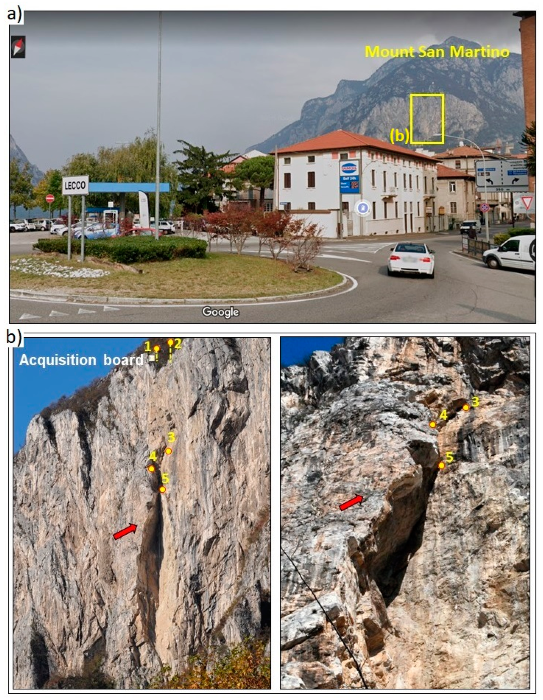
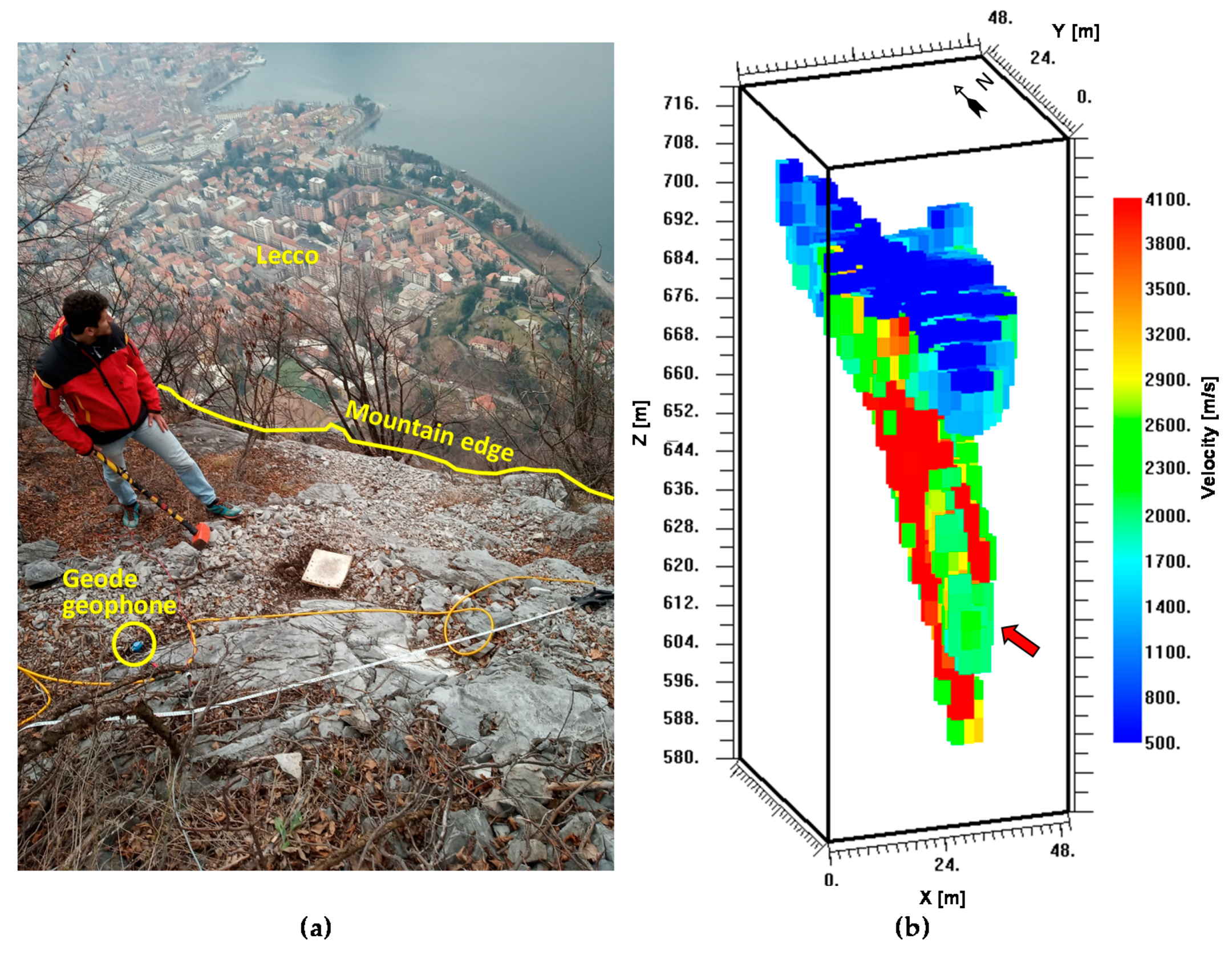
2.1. Study Area

The investigated site is a 330 m high limestone rock face on the southern side of Mount San Martino, as shown in Figure 1a, in the Lombardy region, Northern Italy. The rock face overlooks Lecco city on its northern side and has experienced several rockfalls and collapses in the past. The most tragic event happened on the night between 22 and 23 February 1969. About 15,000 m3 rock blocks were detached from the steep rock face, overwhelming an inhabited building causing the death of seven people and the injury of three people. Since then, the most dangerous area is the partially detached rock pillar close to the 1969 collapse, as shown in Figure 1b, and the instability of the rock face remains a serious threat to Lecco city. Therefore, a microseismic network equipped with five three-component geophones was installed on this rock face in February 2013. The system acquires data with a 1 kHz sampling frequency based on a defined triggering method. The monitoring network also includes a rain gauge for rainfall data and two temperature sensors to measure the air temperature outside and inside a rock fracture, both with a 10 s time interval. Two geophones (Geophones 1 and 2 in Figure 1b) were deployed at the bottom of two boreholes, located on the summit of the rock face where the acquisition board was also installed. Three other geophones (Geophones 3, 4, and 5 in Figure 1b) were installed on the rock face close to the 1969 collapse to efficiently monitor the partially detached rock pillar which is deemed as the zone with a high probability of rockfall risk. Geophone 4 was placed on the top of the unstable rock pillar, while Geophones 3 and 5 were installed on the rock face next to the rock pillar. Therefore, we can compare the difference in the recordings acquired from the unstable rock pillar and rock face. The layout of the geophones was also constrained by the limitation on the number of available channels, and the necessity of performing field installation with a reasonable effort and avoiding excessive risks. More information on data acquisition can be found in the literature [32,35].

2.2. Automatic Classification of Events

In this study, we analyzed a 6-year-long dataset of the microseismic network recorded in the period of February 2013 to December 2018. The dataset was first submitted to an automatic classification procedure proposed by Arosio et al. [32]. The automatic classification algorithm is developed based on linear discriminant analysis (LDA), which is a supervised machine learning approach that can recognize patterns in the available data and then predict future data by using the discovered patterns. More specifically, LDA is a parameter-based classification method that trains data with inputs and outputs to fit a predictive model and then uses this model to classify future data. In the classification algorithm for collected events, input data include 12-dimensional vectors of numbers, which are the signal parameters in time and frequency domains. The outputs of the algorithm are the following five classes of the collected signals:
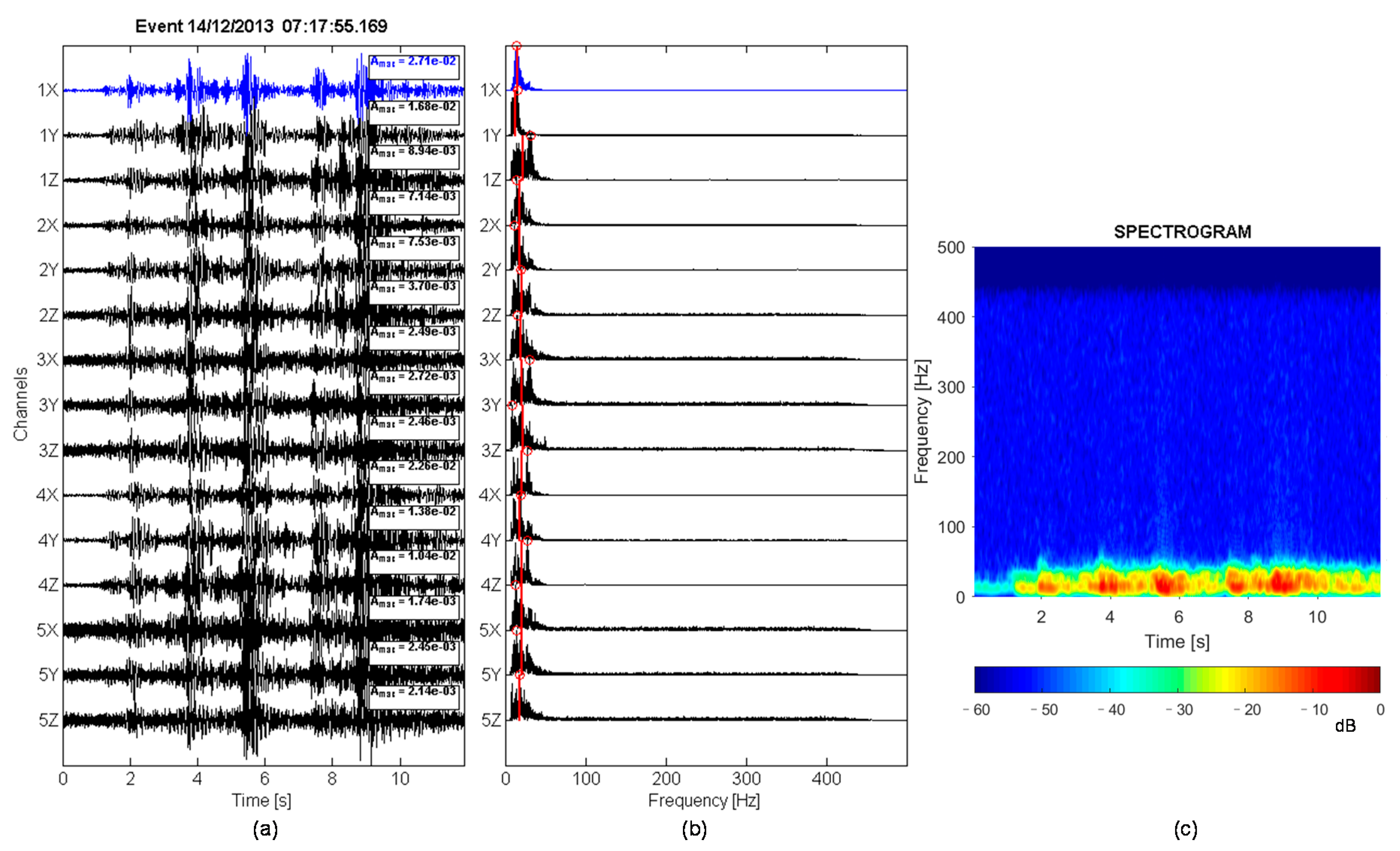
  • Microseismic events likely related to the propagation of fractures inside the rock mass or to rockfalls (MS events);
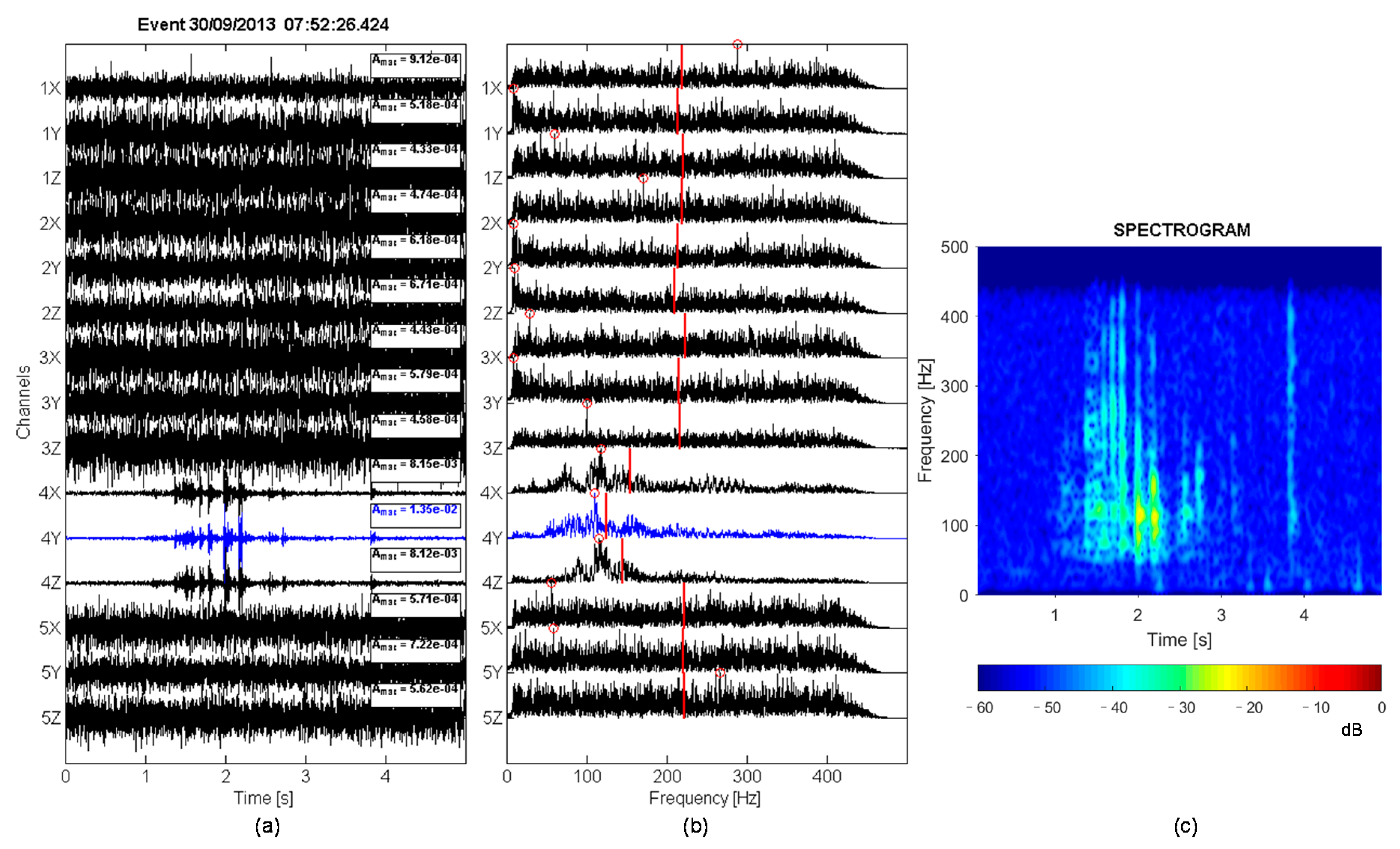
  • Local events related to minor rockfalls generated by small rocks hitting the rock face close to the geophone locations and thus recorded by just a limited number of channels (local events);
  • Broad-band (BB) signals related to impulsive signals with a broad frequency band, mostly generated by thunderstorms (BB signals);
  • Mixed events including both broad-band signals and microseismic events (mixed events);
  • Unclassified noise indicating the signals with unspecified characteristics (unclassified noise).
The five classes of collected signals were already identified during the manual classification process. For each classified event, the corresponding 12 parameters were computed and stored. With the training data of input–output pairs, the predictive model can be searched through the discriminant analysis approach by randomly choosing training datasets of different sizes. The performance of the automatic classification is evaluated by the predefined hit rate (HR) and false alarm rate (FAR). The main goal of the automatic algorithm is to obtain a high HR and a tolerable FAR in order to make the manual quality control unnecessary.
During the monitoring period of about 6 years, the five-class events had different distributions in collected signals. The average number of the annual recorded events was around 3000. The percentage of different events for each year was about 1.6% for microseismic events, 0.6% for local events, 95.0% for BB signals, 1.7% for mixed events, and 1.1% for unclassified noise. Therefore, the preponderant class is BB signals that, however, are quite easy to be distinguished and filtered. The target of our study is the 1.6% of events that belongs to the class of microseismic events, i.e., events that might be generated by fractures or rockfalls.
Figure 2, Figure 3 and Figure 4 illustrate some examples of classified events with their specific features. Both the signals in the time domain and the spectra are normalized trace by trace but the maximum amplitudes recorded in each trace are reported within the small boxes in the time plots to allow amplitude comparisons. Microseismic events possibly related to fracturing procedures within the rock mass, as shown in Figure 2, are generally in the 10–150 Hz frequency range. Their time durations are of a few seconds or less and their spectrograms are often triangular-shaped. As mentioned in several studies (e.g., [18]), attenuation of higher frequencies can be also observed, which is generally caused by the complex fracture distribution inside the rock mass. Microseismic events generated by rockfalls, as shown in Figure 3, might show longer overall time durations and lower frequency bands, especially when the rockfall occurred far from the sensors. The event illustrated in Figure 3 was a known rockfall reported to the local authority and involved a rock volume of around 10 m3. It should be noted that in Figure 2 and Figure 3, the amplitudes recorded by Geophones 3 and 5 are lower than those recorded by Geophone 4. The probable reason, somehow validated by specific ambient noise tests [32], is that amplification phenomena happen to Geophone 4 because it was installed on the top of the partially detached rock pillar. Local events, which are only sensed by a limited number of channels, generally present multiple signals and wider frequency ranges with higher frequency content, as shown in Figure 4. These events are assumed to be related to the impacts of small rocks and most of the local events happened close to Geophone 4 that was installed on the rock pillar exposed to rockfalls from the upper part of the rock face.

2.3. Classification of Microseismic Data

The data were classified by the automatic classification algorithm and we obtained 251 microseismic events. The class of microseismic events was further divided into two subclasses: (1) events likely related to fracturing processes within the rock mass, showing a single pulse in each recording (suspected fracture events); (2) events deemed to be generated by rockfalls, showing a pattern of multiple pulses for each recording (suspected rockfall events). Figure 5a shows two examples of suspected rockfall events and Figure 5b illustrates two examples of suspected fracture events. The red arrows along the recordings in Figure 5a indicate the signals that we planned to pick (four signals for Rockfall 1 and three signals for Rockfall 10).
Being only based on the observation of a single signal versus multiple signals in the recordings, this classification is not rigorous. Records having a single signal could be also generated by a single stone hitting the rock face only once. Vice versa, we cannot exclude the fact that a record with multiple signals might be generated by a complex stress release within the rock mass. Therefore, the sub-classification should be improved by introducing more parameters for the characterization of fractures and rockfalls. On the other hand, if event localization is accurate enough, its results can be used to distinguish rockfalls from fracture events because rockfalls only occur on the rock surface [36]. In this study, 155 suspected fracture events and 96 suspected rockfall events were detected by the sub-classification. Among these events, we selected 20 suspected fracture events and 10 suspected rockfall events with good signal quality to test the localization algorithm as a classification tool. The events were picked manually for localization.

2.4. 3D Seismic Velocity Model

Reliable event location necessitates a detailed description of the velocity distribution within the rock mass [13,17,18,22]. Due to heterogeneities within the rock mass, weathering effects, uneven stress distribution, and fracture location and orientation, the seismic velocity distribution is quite complex and assuming a constant velocity model is quite unrealistic. Since seismic tomography is a helpful tool to estimate the velocity distribution, a tomographic survey was carefully designed and performed on the summit of the rock face [35,37].
Our seismic tomographic survey combined a 24-channel Geode recording system with the permanent microseismic network in order to increase the volume of the rock mass crossed by the seismic rays. A 3D spread consisting of 24 vertical geophones was deployed over the complex topography of the rock summit with about 3 m spacing. An 8 kg hammer was selected as the source due to its flexibility and portability in the harsh environment on the mountain. Twenty-six hammer shots were performed at 12 source positions distributed over the summit of the rock mass, trying to extend as much as possible the rock volume explored by the tomographic survey, as shown in Figure 6a.
In order to further expand the volume crossed by the seismic rays, the data measured in previous source tests with the hammer and seismic gun, including 20 shots performed at five different source positions [35], were also added to the dataset. The extent of the investigation area is 40 × 35 m in the horizontal direction and about 100 m in the vertical direction. The data were picked manually and, from the complete set of 854 seismograms (26 shots × 29 receivers + 20 shots × 5 receivers), we were able to manually pick 503 first-arrival times with an accuracy of about 2 ms. The 3D inversion of these travel times was performed using the simultaneous iterative reconstruction technique (SIRT) [38]. A starting model with a constant velocity of 2000 m/s was used in the inversion. The results revealed a highly heterogeneous velocity distribution within the rock mass, as shown in Figure 6b. The 3D velocity model shows a gradual and remarkable increase in velocity from the summit of the cliff (about 500–1500 m/s) to the lower part of the rock mass near Geophones 3, 4, and 5 (>3000 m/s), with some areas of the rock mass showing higher velocities (>4000 m/s). More specifically, we can observe a relatively low-velocity area (2200–3100 m/s) corresponding to the upper part of the partially detached rock pillar (the area indicated by red arrow in Figure 6b) compared to the higher velocity (4000 m/s) in the neighboring rock mass. Two sensitivity tests using the checkerboard resolution test and restoring resolution test were performed to evaluate the resolution and stability of the inversion. According to the results obtained from these two sensitivity tests, the 3D velocity model based on the inversion can be a reliable representation of the velocity distribution within the rock mass with the best resolution of 6 × 6 m in the horizontal direction and 8 m in the vertical direction [35]. The main advantage of using this velocity model rather than a constant velocity, which is commonly used when no velocity information is available, is the expected improvement of the localization accuracy. This is further discussed in the following section.

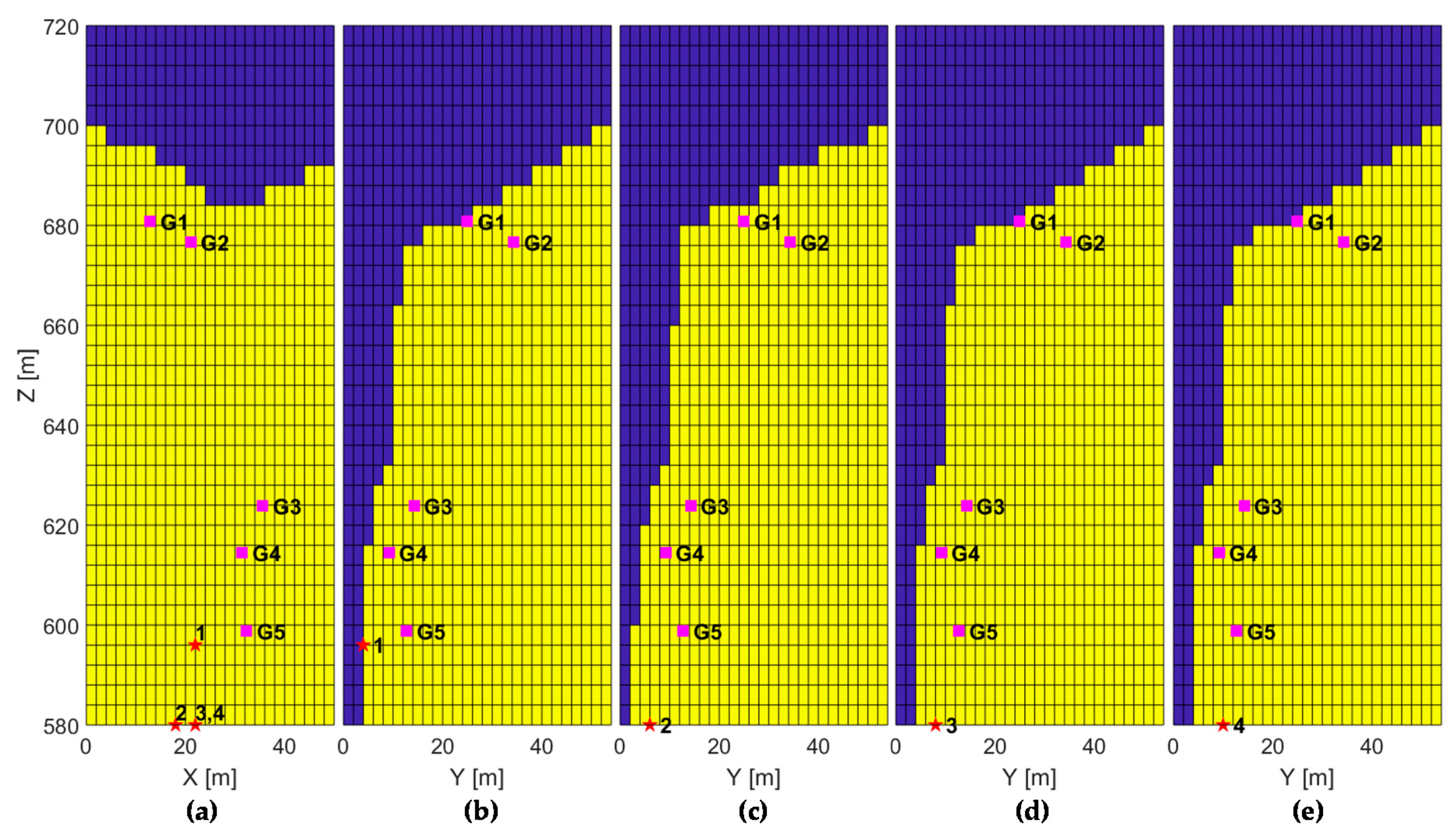
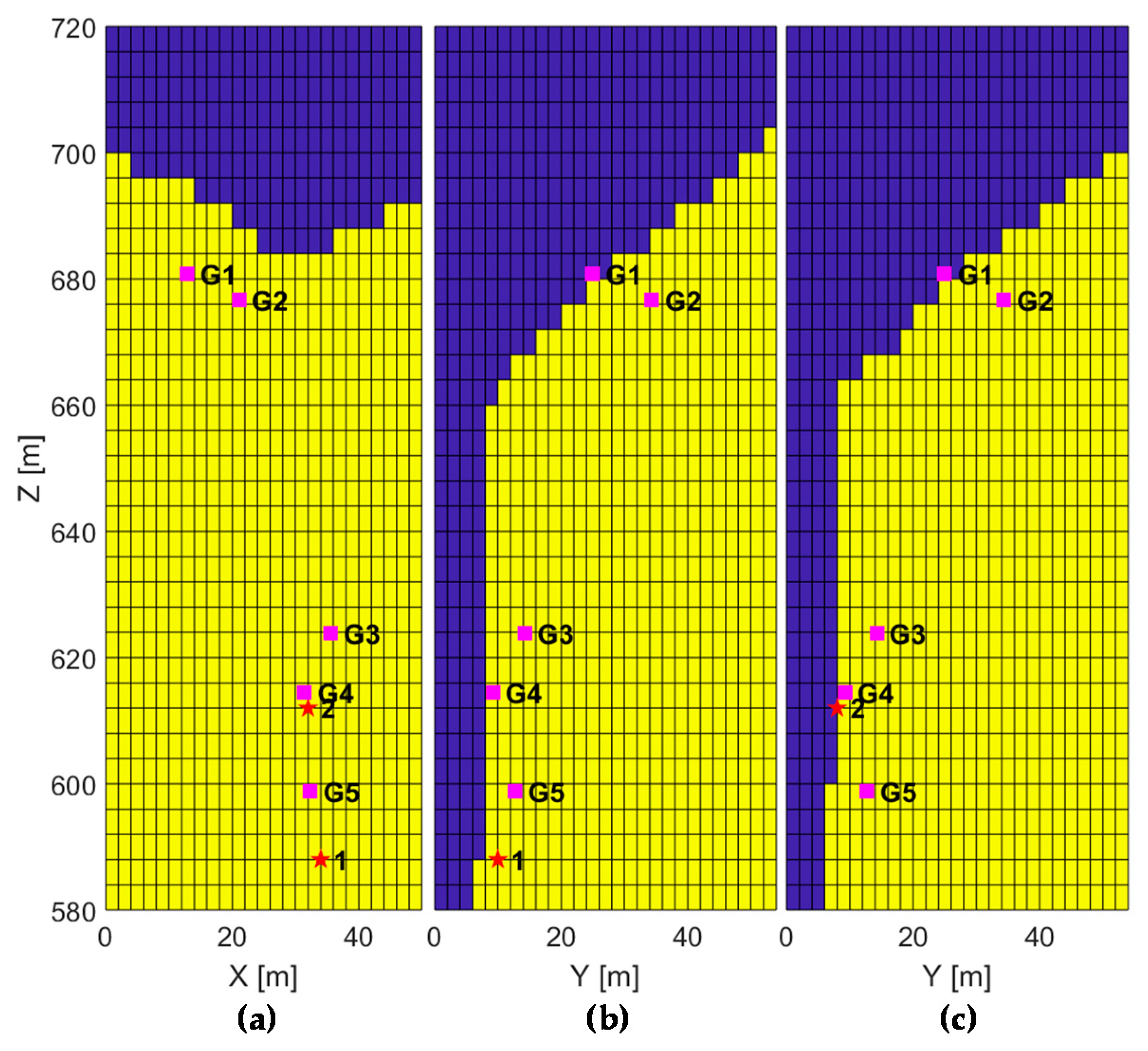
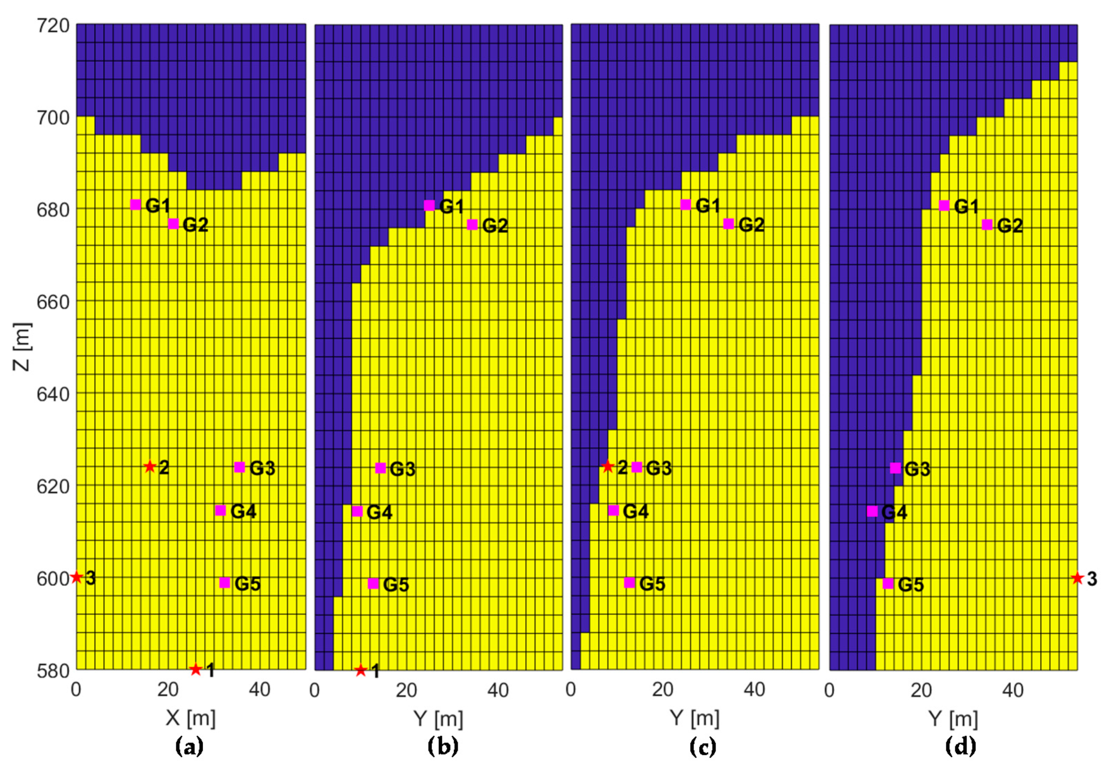
2.5. Localization Method and Location Accuracy

A direct global grid search approach, which is commonly applied to locate hypocenters of earthquakes [39], was selected to localize the events. We used the equal differential time (EDT) method [40] to define the misfit function. An L2-norm misfit function was used. The source position can be estimated by searching the grid point which minimizes the global misfit between the observed and calculated differential times. The observed arrival times were obtained from the picking and the calculated travel times were computed using a bending ray-tracing method within a 3D grid velocity model.
We performed a source re-localization test to assess and quantify the convenience of using a 3D velocity model rather than using a constant velocity model. The data excluded from the tomographic inversion and selected for the localization test consist of eight hammer shots characterized by a relatively higher signal to noise ratio (SNR) so that the first arrival time picking is expected to be reliable enough. These eight shots have 5 first-arrival times from all the geophones available for localization. Although 4 first-arrival times are the theoretical minimum number of data to make a location, we decided to work with a minimum of 5 first-arrival times to have a minimum redundancy in our data to contrast the noise and to ensure the best location accuracy achievable with our current network. The 3D velocity model and the constant velocity model were used to localize the shots with the 5 geophones of the microseismic network to assess the accuracy improvement resulting from the 3D model and the location accuracy that we can generally expect from the monitoring system. The constant velocity is 1703 m/s, which was obtained from the least squares fitting of the data used in the tomographic inversion. The location results show that the average localization errors of the eight shots were reduced significantly from 39 m to 15 m when using the 3D velocity model rather than a constant velocity field [35]. This localization method will be used in the following section to locate the selected rockfall events and fracture events.

3. Results and Discussion

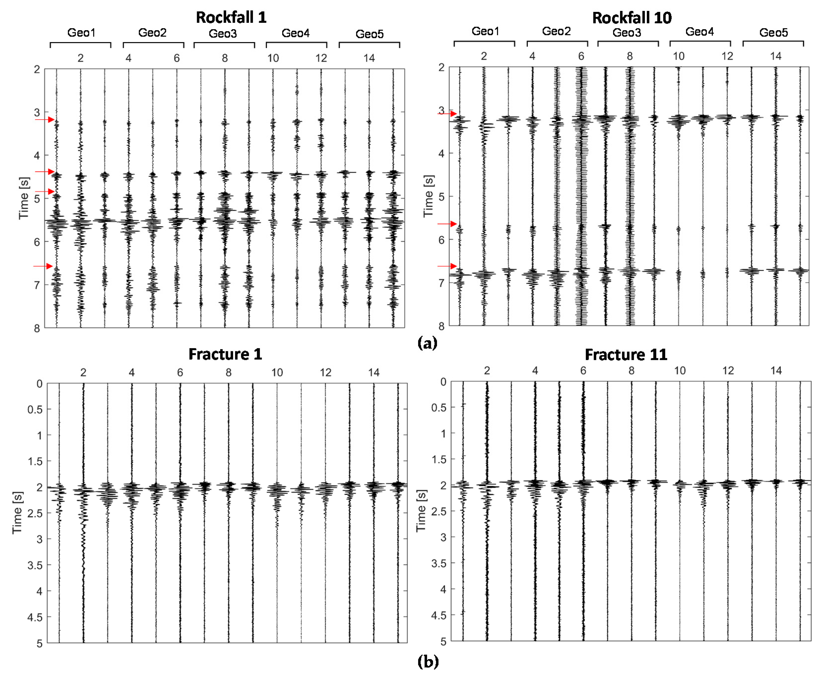
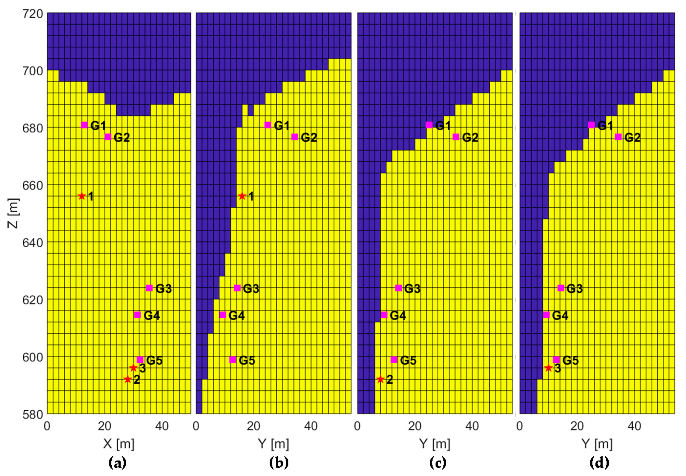
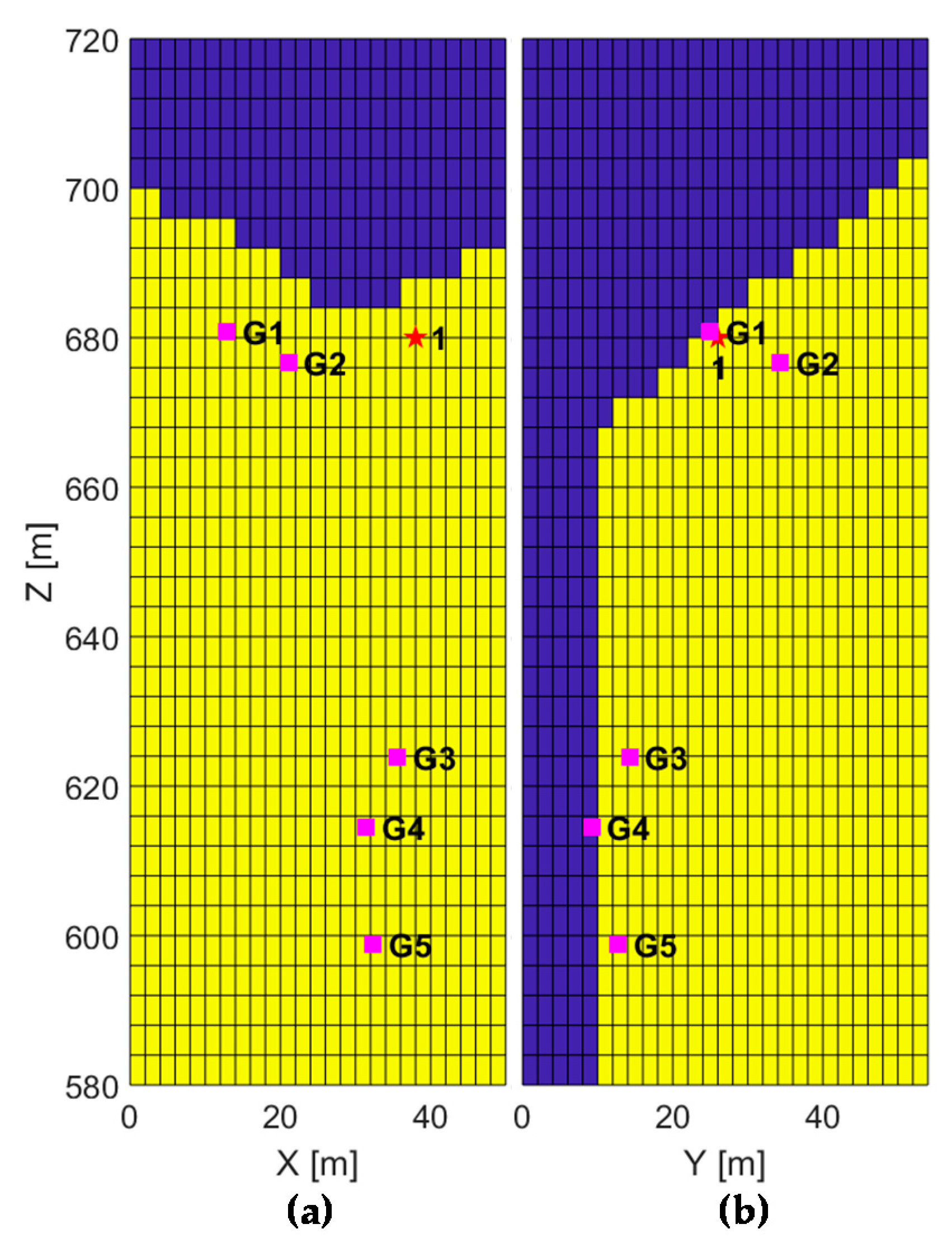
3.1. Location of Rockfall Events

Rockfall events generally consist of a sequence of short signals like the examples shown in Figure 5a. For each rockfall event, only the signals having manual picks from all the five geophones were used in the localization procedure. The location results of 10 rockfall events are summarized in Table 1.
For 7 events (Rockfall events 1–3, 5–6, 9–10) among the 10 suspected rockfalls, all the signals were located on or near the rock face, i.e., within a distance from the rock face shorter than the average expected location accuracy (about 15 m), confirming the preliminary classification. Similarly, two events (Rockfall events 4 and 7) were confirmed as rockfalls because for both events one signal was located at the vertical boundary of the model, which corresponds to an event occurring outside the monitored area, and all other signals were located on or near the rock face. The last suspected rockfall (Rockfall event 8) consists of seven signals—three of them were located on or near the rock face, three others were located at the boundary of the model (events occurring out of the monitored area), and one signal was surprisingly located in the middle of the model. Thus, the most probable interpretation is a rockfall with one signal among seven that was wrongly located due to picking errors; although, in principle, we cannot exclude an improbable combination of a rockfall and a fracture event. On the whole, for all the events in Table 1, the hypocenter location supports the classification as rockfalls and significantly increases the level of confidence of the classification. The last column in Table 1 refers to the rockfall type, which is additional information that we can derive from the analysis of the number of recorded signals combined with their time of occurrence and their location. Based on that, rockfall events can be sub-classified into four rockfall types:
  • Rockfall events that were generated by only one falling stone bouncing on the rock face (Single);
  • Rockfall events that involve more than one stone (Multiple);
  • Rockfall events in which the number of involved stones is uncertain considering the location accuracy (Uncertain);
  • Rockfall events that occurred on the rock surface at the summit of the rock face (Summit debris noise).
Figure 7, Figure 8, Figure 9, Figure 10 and Figure 11 show several examples of the location results for rockfall events. They are illustrated by showing a vertical slice in the front view (Y = 32 m) and a vertical slice cut through the location of each signal in the side view to show the distance from the rock face. The 3D model consists of a 2 × 2 × 4 m grid. The blue area is the air, and the yellow area is the rock mass. Pink squares indicate the five 3C geophones numbered in the descending order for elevation, projected on the slice. Red stars indicate the event locations projected on the slice and numbers are used to order the signals according to the arrival times.
For Rockfall event 1, as shown in Figure 7, the first signal was located at the position which is slightly below Geophone 5 in the vertical direction and at the boundary of the velocity model in the horizontal direction. This indicates that it is close to the rock face. The other three signals were located at the lower boundary of the model near the rock face and this is consistent with the expectation because these three signals likely hit the rock face at points that are below the velocity model. We can assume that Rockfall event 1 was generated by a single stone bouncing on the rock slope four times. For Rockfall event 9, as shown in Figure 8, the first signal was located at the point below Geophone 5 and the second signal was located at the point just below Geophone 4 in the front view. In the side view, both signals were located on or near the rock face. According to arrival times and locations, we have to assume that Rockfall event 9 was generated by two different stones. For Rockfall event 7, as shown in Figure 9, the first signal was located at the lower boundary of the model and near the rock face. The second signal was located left of Geophone 3 and on the rock face. On the contrary, the third signal was located on the vertical boundary of the model and far from the rock face of the monitored area. The possible explanation is that Rockfall event 7 was generated by three stones; one hitting the rock face at a point below the model, another one hitting a point on the rock face left of Geophone 3, and finally a third one occurring at a point which is outside the monitored area so that it was located at the left boundary of the front view. For Rockfall event 5, as shown in Figure 10, the first signal was located at a point in the middle of the model and near the rock face. The second and third signals were both located at points close to Geophone 5 and near the rock face. Considering the location accuracy, the real position of the third signal might be either higher or lower than that of the second signal. Therefore, the number of stones involved in this rockfall event is uncertain—all three signals could be generated by a single stone or the first two signals were generated by one stone and the third signal was generated by another stone. Finally, Rockfall event 6 included multiple signals but only one signal could be picked on all five geophones. The picked signal was located on the rock surface at the summit of the rock face, as shown in Figure 11. We can assume that this event was generated by a movement of stones on the slope of debris covering the summit of the rock face. This also explains the weak signals that were not recorded with sufficient energy to be picked on all the five sensors.
On the whole, the location results for the suspected rockfall events almost meet our expectations. We can observe that seven out of ten rockfall events have all the signals located on or near the rock face. For two events, we were able to exclude some events occurring outside the monitored area, which were the signals located on the lateral model boundaries, and to locate other events on or near the rock face. In only one case among the ten events, we observed a signal that was unexpectedly located within the rock mass. This might be the result of a picking error or an improbable mixed event where a signal generated by a fracture occurs in combination with a rockfall. Thus, according to the localization results, we can confirm the rockfall classification for these events. It should be noted that based on the hypocenter locations and the order of arrival times, the successive signals in a rockfall event were generated by more than one falling stone in many cases. This indicates that multiple sources are often involved in the recordings of rockfall events.

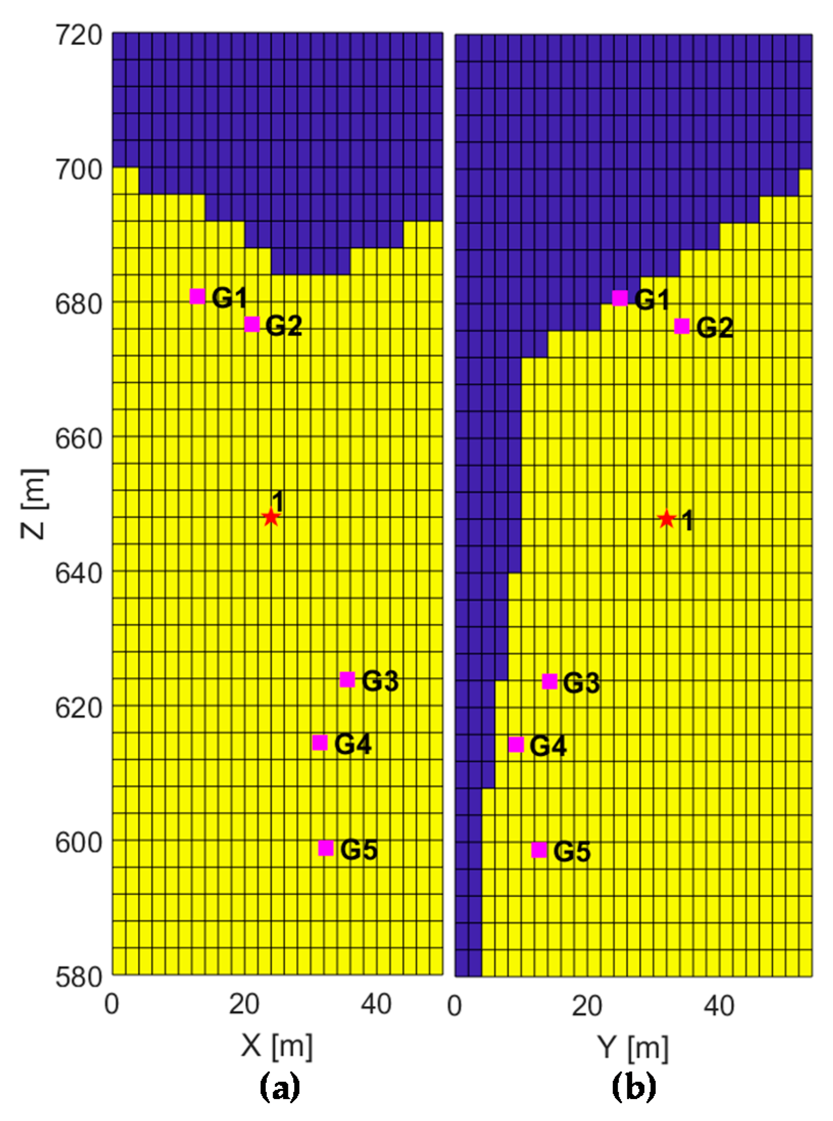
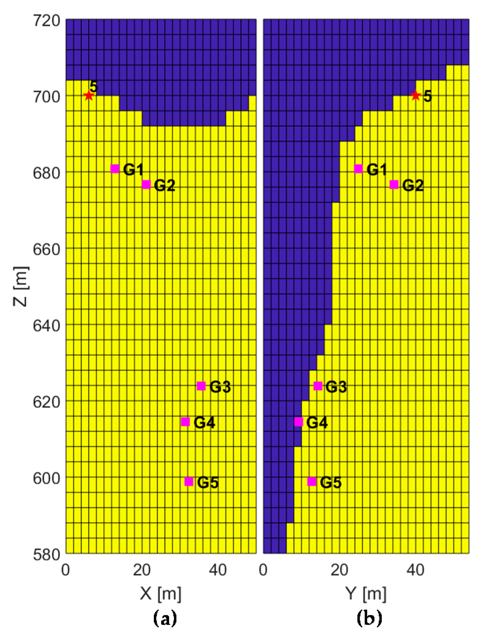
3.2. Location of Fracture Events

Suspected fracture events have only one signal in the recordings. As mentioned before, the events with pickings from all five geophones were used for localization. Table 2 summarizes the location results for 20 selected fracture events. Based on the hypocenter locations, these fracture events could be reclassified into five groups: events that are located inside the rock mass (Fracture); events that are located on the rock surface at the summit of the rock face and are probably related to the movement of the debris covering the summit (Rockfall); events that are located on the vertical boundaries of the model (Far event); events that are located near the rock face so that they are likely generated by a fracture although we cannot exclude a single stone rockfall hitting the rock face only once and then disappearing without generating any other signal from a lower point below the monitored area (Suspected fracture); and events that are located at the lower boundary of the model near the rock face so that we suspect that they are fracture events occurring within the lower section of the unstable area of the rock mass, i.e., the lower part of the unstable rock pillar, although we cannot exclude the case of a single stone hitting the rock face only once at a point located below the monitored area (Suspected fracture (outside the area)).
Figure 12, Figure 13, Figure 14, Figure 15 and Figure 16 depict some examples of different classified events with their location features. Fracture event 1, as shown in Figure 12, is a typical fracture that was located inside the rock mass and not close to the rock face. Furthermore, considering the location accuracy, it can be excluded from the rockfalls. This event should be related to fracturing generation within the rock mass. Fracture event 5, as shown in Figure 13, is an example of a rockfall. The hypocenter was located on the rock surface at the summit of the rock face. Since the summit of the rock slope is covered by rock debris, we assume that the probability that this event was produced by movement of rock debris on the surface is higher than the probability that it was produced by a near-surface fracture. Fracture event 19, as shown in Figure 14, is an example of a far event. The hypocenter location was on the vertical boundary of the model and far away from the rock face. We can assume that this event was generated outside the monitored area. This type of event is not related to the stability of the rock cliff in the monitored area. Fracture event 13, as shown in Figure 15, is an example of a suspected fracture. Although the hypocenter location is within the rock mass, the distance from the rock face is within the expected location accuracy. As a result, the class of this event is still uncertain—it might be either a rockfall or a fracture near the rock face. This is an example showing the importance of further improving the location accuracy in order to distinguish fractures close to the rock face from rockfalls. Fracture event 20, as shown in Figure 16, is an example of a suspected fracture (outside the area). The event was located at the lower boundary of the model and within a short distance from the rock face. Thus, the class of this event is still uncertain—it might be either a stone hitting the rock face at a point below the monitored area or a near-surface fracture generated inside the rock mass below the monitored area.
Fractures are considered as the most valuable events related to the instability of the rock cliff. According to the localization results for 20 selected fracture events, only 4 events were confirmed as fractures and 6 events were reclassified as rockfalls or events generated far from the monitored area. The remaining ten events are still suspected fractures, although we cannot exclude the possibility that they are rockfalls and this type of uncertainty cannot be solved until we improve the location accuracy. On the whole, the location of hypocenters was quite useful to update our preliminary classification by reclassifying some of the initially suspected fractures as rockfalls or far events.

4. Conclusions

A microseismic monitoring system has been installed on an unstable rock face for early warning purposes. Due to the importance of fracture events in an early warning system, the classification of microseismic events is required to distinguish events generated by fracture propagation from rockfalls. Therefore, a classification procedure based on hypocenter location was proposed and implemented by using a subset of high-quality data to validate its efficiency. The selected subset includes 10 suspected rockfall events with multiple signals in the recordings and 20 suspected fracture events with a single signal. The results of the event location fairly agreed with our preliminary classification of rockfall events. Most of the signals in rockfall events were located on or near the rock face and thus confirming the initial classification. However, for fracture events, only 4 out of 20 events were located inside the rock mass at such a distance from the rock face that they could not be confused with rockfalls. Further improvements in location accuracy are necessary to distinguish suspected fracture events located close to the rock face from rockfalls. Such an ambiguity occurred for 10 out of the 20 events considered in this analysis. The location accuracy can be improved by expanding the current network by adding more geophones in the investigated area. With an improved geophone coverage in the monitoring area, the location problem will be better constrained. The study about the expansion of the current monitoring network is in progress and the expansion is planned for the near future. It is interesting to note that some classifications (4 out of 20) had to be revised according to location results, which demonstrated that these events were actually of a rockfall nature while they were initially classified as fractures. This is typically the case of single events that were located on the rock surface at the summit of the rock face. Hypocenter location is also fundamental to identify events generated outside the monitored area (2 out of 20 in this analysis). Overall, although the current location accuracy is not small enough to distinguish rockfalls from rock cracks occurring near the exposed face of the rock mass, the location algorithm can be successfully used to improve the classification procedure by distinguishing events occurring in the monitored area from rockfalls or other events occurring far from the monitored areas and by confirming or reclassifying the events whenever their location is unquestionably proving the nature of the event. Thus, this feasibility study shows that the hypocenter location is a promising method to improve the final classification of microseismic events.

Author Contributions

Conceptualization, Z.Z. and L.Z.; methodology, Z.Z. and L.Z.; software, Z.Z. and D.A.; validation, Z.Z., L.Z., A.H., and D.A.; formal analysis, Z.Z. and L.Z.; investigation, Z.Z., L.Z., A.H., and D.A.; resources, Z.Z., L.Z., A.H., and D.A.; data curation, Z.Z., L.Z., and D.A.; writing—original draft preparation, Z.Z.; writing—review and editing, Z.Z., L.Z., A.H., and D.A.; visualization, Z.Z. and L.Z.; supervision, L.Z.; project administration, L.Z.; funding acquisition, Z.Z. and L.Z. All authors have read and agreed to the published version of the manuscript.

Funding

This research was funded by China Scholarship Council (CSC), grant number 201606420051, to support Zhiyong Zhang during his research activities in Italy. The research activities have been partially funded by the municipality of the city of Lecco and by the provincial authority of Lecco.

Institutional Review Board Statement

Not applicable.

Informed Consent Statement

Not applicable.

Data Availability Statement

Restrictions apply to the availability of these data. Data are available from the authors upon request with the permission of local authorities (Municipality of Lecco).

Acknowledgments

We are grateful to Stefano Munda and Marco Taruselli for their technical assistance during the tomographic survey on the rock cliff. The authors wish to acknowledge the journal editor and the reviewers for their constructive reviews that improved the quality of the manuscript.

Conflicts of Interest

The authors declare no conflict of interest.

References

  1. Hungr, O.; Leroueil, S.; Picarelli, L. The Varnes classification of landslide types, an update. Landslides 2014, 11, 167–194. [Google Scholar] [CrossRef]
  2. Supper, R.; Ottowitz, D.; Jochum, B.; Kim, J.H.; Römer, A.; Baron, I.; Pfeiler, S.; Lovisolo, M.; Gruber, S.; Vecchiotti, F. Geoelectrical monitoring: An innovative method to supplement landslide surveillance and early warning. Near Surf. Geophys. 2014, 12, 133–150. [Google Scholar] [CrossRef] [Green Version]
  3. Arosio, D.; Munda, S.; Tresoldi, G.; Papini, M.; Longoni, L.; Zanzi, L. A customized resistivity system for monitoring saturation and seepage in earthen levees: Installation and validation. Open Geosci. 2017, 9, 457–467. [Google Scholar] [CrossRef]
  4. Taruselli, M.; Arosio, D.; Longoni, L.; Papini, M.; Corsini, A.; Zanzi, L. Rock Stability as Detected by Seismic Noise Recordings-Three Case Studies. In Proceedings of the 24th European Meeting of Environmental and Engineering Geophysics, Porto, Portugal, 9–13 September 2018. [Google Scholar]
  5. Hojat, A.; Arosio, D.; Longoni, L.; Papini, M.; Tresoldi, G.; Zanzi, L. Installation and validation of a customized resistivity system for permanent monitoring of a river embankment. In Proceedings of the EAGE-GSM 2nd Asia Pacific Meeting on Near Surface Geoscience and Engineering, Kuala Lumpur, Malaysia, 22–26 April 2019. [Google Scholar]
  6. Hojat, A.; Arosio, D.; Ivanov, V.I.; Longoni, L.; Papini, M.; Scaioni, M.; Tresoldi, G.; Zanzi, L. Geoelectrical characterization and monitoring of slopes on a rainfall-triggered landslide simulator. J. Appl. Geophys. 2019, 170, 103844. [Google Scholar] [CrossRef]
  7. Cochran, E.S.; Wolin, E.; McNamara, D.E.; Yong, A.; Wilson, D.; Alvarez, M.; Van Der Elst, N.; McClain, A.; Steidl, J. The U.S. Geological Survey’s Rapid seismic array deployment for the 2019 ridgecrest earthquake sequence. Seismol. Res. Lett. 2020, 91, 1952–1960. [Google Scholar] [CrossRef]
  8. Hojat, A.; Arosio, D.; Ivanov, V.I.; Loke, M.H.; Longoni, L.; Papini, M.; Tresoldi, G.; Zanzi, L. Quantifying seasonal 3D effects for a permanent electrical resistivity tomography monitoring system along the embankment of an irrigation canal. Near Surf. Geophys. 2020, 18, 427–443. [Google Scholar] [CrossRef]
  9. Searcy, C.K.; Power, J.A. Seismic character and progression of explosive activity during the 2016–2017 eruption of Bogoslof volcano, Alaska. Bull. Volcanol. 2020, 82, 12. [Google Scholar] [CrossRef]
  10. Ziwu, F.D.; Doser, D.I.; Schinagel, S.M. A geophysical study of the Castle Mountain Fault, southcentral Alaska. Tectonophysics 2020, 789, 228567. [Google Scholar] [CrossRef]
  11. Huang, C.J.; Yin, H.Y.; Chen, C.Y.; Yeh, C.H.; Wang, C.L. Ground vibrations produced by rock motions and debris flows. J. Geophys. Res. Earth Surf. 2007, 112, 1–20. [Google Scholar] [CrossRef] [Green Version]
  12. Deparis, J.; Jongmans, D.; Cotton, F.; Baillet, L.; Thouvenot, F.; Hantz, D. Analysis of rock-fall and rock-fall avalanche seismograms in the French Alps. Bull. Seismol. Soc. Am. 2008, 98, 1781–1796. [Google Scholar] [CrossRef] [Green Version]
  13. Helmstetter, A.; Garambois, S. Seismic monitoring of Schilienne rockslide (French Alps): Analysis of seismic signals and their correlation with rainfalls. J. Geophys. Res. Earth Surf. 2010, 115, 1–15. [Google Scholar] [CrossRef]
  14. Burjánek, J.; Gassner-Stamm, G.; Poggi, V.; Moore, J.R.; Fäh, D. Ambient vibration analysis of an unstable mountain slope. Geophys. J. Int. 2010, 180, 820–828. [Google Scholar] [CrossRef] [Green Version]
  15. Hibert, C.; Mangeney, A.; Grandjean, G.; Shapiro, N.M. Slope instabilities in Dolomieu crater, Réunion Island: From seismic signals to rockfall characteristics. J. Geophys. Res. Earth Surf. 2011, 116, 1–18. [Google Scholar] [CrossRef] [Green Version]
  16. Dietze, M.; Mohadjer, S.; Turowski, J.M.; Ehlers, T.A.; Hovius, N. Seismic monitoring of small alpine rockfalls-validity, precision and limitations. Earth Surf. Dyn. 2017, 5, 653–668. [Google Scholar] [CrossRef] [Green Version]
  17. Colombero, C.; Comina, C.; Vinciguerra, S.; Benson, P.M. Microseismicity of an unstable rock mass: From field monitoring to laboratory testing. J. Geophys. Res. Solid Earth 2018, 123, 1673–1693. [Google Scholar] [CrossRef] [Green Version]
  18. Spillmann, T.; Maurer, H.; Green, A.G.; Heincke, B.; Willenberg, H.; Husen, S. Microseismic investigation of an unstable mountain slope in the Swiss Alps. J. Geophys. Res. Solid Earth 2007, 112, 1–25. [Google Scholar] [CrossRef]
  19. Manconi, A.; Picozzi, M.; Coviello, V.; De Santis, F.; Elia, L. Real-time detection, location, and characterization of rockslides using broadband regional seismic networks. Geophys. Res. Lett. 2016, 43, 6960–6967. [Google Scholar] [CrossRef]
  20. Provost, F.; Hibert, C.; Malet, J.P. Automatic classification of endogenous landslide seismicity using the Random Forest supervised classifier. Geophys. Res. Lett. 2017, 44, 113–120. [Google Scholar] [CrossRef]
  21. Feng, L.; Pazzi, V.; Intrieri, E.; Gracchi, T.; Gigli, G.; Tucci, G. Rockfall localization from seismic polarization considering multiple triaxial geophones and frequency bands. J. Mt. Sci. 2020, 17, 1541–1552. [Google Scholar] [CrossRef]
  22. Walter, M.; Joswig, M. Seismic characterization of slope dynamics caused by softrock-landslides: The Super-Sauze case study. In Proceedings of the International Conference on Landslide Processes: From Geomorphologic Mapping to Dynamic Modelling, Strasbourg, France, 6–7 February 2009. [Google Scholar]
  23. Arosio, D.; Zanzi, L.; Longoni, L.; Papini, M. Microseismic monitoring of an unstable rock face—Preliminary signal classification. In Proceedings of the Near Surface Geoscience 2015—21st European Meeting of Environmental and Engineering Geophysics, Turin, Italy, 6–10 September 2015; pp. 1–4. [Google Scholar]
  24. Senfaute, G.; Duperret, A.; Lawrence, J.A. Micro-seismic precursory cracks prior to rock-fall on coastal chalk cliffs: A case study at Mesnil-Val, Normandie, NW France. Nat. Hazards Earth Syst. Sci. 2009, 9, 1625–1641. [Google Scholar] [CrossRef]
  25. Got, J.L.; Mourot, P.; Grangeon, J. Pre-failure behaviour of an unstable limestone cliff from displacement and seismic data. Nat. Hazards Earth Syst. Sci. 2010, 10, 819–829. [Google Scholar] [CrossRef]
  26. Bottelin, P.; Jongmans, D.; Daudon, D.; Mathy, A.; Helmstetter, A.; Bonilla-Sierra, V.; Cadet, H.; Amitrano, D.; Richefeu, V.; Lorier, L.; et al. Seismic and mechanical studies of the artificially triggered rockfall at the Mount Néron (French Alps, December 2011). Nat. Hazards Earth Syst. Sci. Discuss. 2014, 2, 1505–1557. [Google Scholar] [CrossRef]
  27. Arosio, D.; Longoni, L.; Papini, M.; Zanzi, L. Analysis of microseismic activity within unstable rock slopes. In Modern Technologies for Landslide Monitoring and Prediction; Scaioni, M., Ed.; Springer: Berlin/Heidelberg, Germany, 2015; pp. 141–154. [Google Scholar]
  28. Taruselli, M.; Arosio, D.; Longoni, L.; Papini, M.; Zanzi, L. Raspberry Shake Sensor Field Tests for Unstable Rock Monitoring. In Proceedings of the 1st Conference on Geophysics for Infrastructure Planning Monitoring and BIM, The Hague, The Netherlands, 8–12 September 2019. [Google Scholar]
  29. Amitrano, D.; Arattano, M.; Chiarle, M.; Mortara, G.; Occhiena, C.; Pirulli, M.; Scavia, C. Microseismic activity analysis for the study of the rupture mechanisms in unstable rock masses. Nat. Hazards Earth Syst. Sci. 2010, 10, 831–841. [Google Scholar] [CrossRef] [Green Version]
  30. Levy, C.; Jongmans, D.; Baillet, L. Analysis of seismic signals recorded on a prone-to-fall rock column (Vercors massif, French Alps). Geophys. J. Int. 2011, 186, 296–310. [Google Scholar] [CrossRef] [Green Version]
  31. Colombero, C. Microseismic Strategies for Characterization and Monitoring of an Unstable Rock Mass. Ph.D. Thesis, University of Turin, Turin, Italy, 2017. [Google Scholar]
  32. Arosio, D.; Longoni, L.; Papini, M.; Boccolari, M.; Zanzi, L. Analysis of microseismic signals collected on an unstable rock face in the Italian Prealps. Geophys. J. Int. 2018, 213, 475–488. [Google Scholar] [CrossRef] [Green Version]
  33. Feng, L.; Pazzi, V.; Intrieri, E.; Gracchi, T.; Gigli, G. Joint detection and classification of rockfalls in a microseismic monitoring network. Geophys. J. Int. 2020, 222, 2108–2120. [Google Scholar] [CrossRef]
  34. Tonnellier, A.; Helmstetter, A.; Malet, J.P.; Schmittbuhl, J.; Corsini, A.; Joswig, M. Seismic monitoring of soft-rock landslides: The Super-Sauze and Valoria case studies. Geophys. J. Int. 2013, 193, 1515–1536. [Google Scholar] [CrossRef] [Green Version]
  35. Zhang, Z.; Arosio, D.; Hojat, A.; Zanzi, L. Tomographic experiments for defining the 3D velocity model of an unstable rock slope to support microseismic event interpretation. Geosciences 2020, 10, 327. [Google Scholar] [CrossRef]
  36. Zhang, Z.; Arosio, D.; Hojat, A.; Zanzi, L. Refining microseismic event classification through hypocentre location. In Proceedings of the EAGE 3rd Asia Pacific Meeting Near Surface Geoscience & Engineering, Chiang Mai, Thailand, 2–5 November 2020. [Google Scholar]
  37. Zhang, Z.; Arosio, D.; Hojat, A.; Taruselli, M.; Zanzi, L. Construction of a 3D velocity model for microseismic event location on a monitored rock slope. In Proceedings of the EAGE-GSM 2nd Asia Pacific Meeting on Near Surface Geoscience and Engineering, Kuala Lumpur, Malaysia, 22–26 April 2019. [Google Scholar]
  38. Peterson, J.E.; Paulsson, B.N.P.; McEvilly, T.V. Applications of algebraic reconstruction techniques to crosshole seismic data. Geophysics 1985, 50, 1566–1580. [Google Scholar] [CrossRef]
  39. Lomax, A.; Michelini, A.; Curtis, A. Earthquake location, direct, global-search methods. In Encyclopedia of Complexity and Systems Science; Meyers, R.A., Ed.; Springer: New York, NY, USA, 2009; pp. 2449–2473. [Google Scholar]
  40. Font, Y.; Kao, H.; Lallemand, S.; Liu, C.S.; Chiao, L.Y. Hypocentre determination offshore of eastern Taiwan using the maximum intersection method. Geophys. J. Int. 2004, 158, 655–675. [Google Scholar] [CrossRef] [Green Version]
Figure 1. The study site in the southern part of Mount San Martino. (a) View of Mount San Martino from Lecco city. The yellow rectangle indicates the monitored area where the monitoring network was deployed. (b) Rock face with the positions of the five geophones and the acquisition board of the microseismic monitoring system. The red arrow indicates the partially detached pillar below Geophone 4.
Geosciences 11 00037 g001
Figure 2. Example of microseismic (MS) events likely related to fracture propagation. (a) Signals recorded by 15 channels (with 5 three-component geophones) with the maximum absolute amplitude written inside the rectangle. The channel in blue color has the maximum absolute amplitude among all 15 channels. (b) Fourier spectra (red circles and red vertical lines present the positions of the peak and centroid of the amplitude spectrum in the channels, respectively). (c) Spectrogram generated by stacking the spectrograms of all channels.
Geosciences 11 00037 g002
Figure 3. Example of MS events related to a reported rockfall. (a) Signals recorded by 15 channels. (b) Fourier spectra. (c) Spectrogram generated by stacking the spectrograms of all channels.
Geosciences 11 00037 g003
Figure 4. Example of local events. (a) Signals recorded by 15 channels. (b) Fourier spectra. (c) Spectrogram generated by stacking the spectrograms of all channels.
Geosciences 11 00037 g004
Figure 5. Microseismic signals recorded by the five 3C-geophones from (a) two suspected rockfalls (red arrows indicate the signals selected for picking and localization), and (b) two suspected fracture events.
Geosciences 11 00037 g005
Figure 6. (a) A picture of the tomographic survey showing one of the hammer shot positions. (b) Velocity model obtained from 3D tomographic inversion using a 2 × 2 × 4 m grid. Colored blocks indicate the velocity field in the rock mass crossed by rays. The red arrow indicates the partially detached pillar on top of which Geophone 4 is installed.
Geosciences 11 00037 g006
Figure 7. Location results for Rockfall event 1 (Single) presented on vertical slices. (a) Vertical slice in the front view (Y = 32 m). The blue area is the air, and the yellow area is the rock mass. Pink squares indicate the five 3C geophones projected on the slice. Red stars indicate the event locations projected on the slice and numbers are used to order the signals according to the arrival times. (be) Vertical slices cutting through the location of each signal in the side view to show the distance between the hypocenter location and the rock face.
Geosciences 11 00037 g007
Figure 8. Location results for Rockfall event 9 (Multiple) presented on vertical slices in the front view (a) and side views (b,c). The blue area is the air, and the yellow area is the rock mass. Pink squares indicate the five 3C geophones projected on the slice. Red stars indicate the event locations projected on the slice and numbers are used to order the signals according to the arrival times.
Geosciences 11 00037 g008
Figure 9. Location results for Rockfall event 7 (Multiple) presented on vertical slices in the front view (a) and side views (bd). The blue area is the air, and the yellow area is the rock mass. Pink squares indicate the five 3C geophones projected on the slice. Red stars indicate the event locations projected on the slice and numbers are used to order the signals according to the arrival times.
Geosciences 11 00037 g009
Figure 10. Location results for Rockfall event 5 (Uncertain) presented on vertical slices in the front view (a) and side views (bd). The blue area is the air, and the yellow area is the rock mass. Pink squares indicate the five 3C geophones projected on the slice. Red stars indicate the event locations projected on the slice and numbers are used to order the signals according to the arrival times.
Geosciences 11 00037 g010
Figure 11. Location results for Rockfall event 6 (Summit debris noise) presented on vertical slices in the front view (a) and side view (b). The blue area is the air, and the yellow area is the rock mass. Pink squares indicate the five 3C geophones projected on the slice. Red stars indicate the event locations projected on the slice and numbers are used to order the signals according to the arrival times.
Geosciences 11 00037 g011
Figure 12. Location results for Fracture event 1 (Fracture) presented on vertical slices in the front view (a) and side view (b). The blue area is the air, and the yellow area is rock mass. Pink squares indicate the five 3C geophones projected on the slice. Red stars indicate the event locations projected on the slice. Both slices cross the event location.
Geosciences 11 00037 g012
Figure 13. Location results for Fracture event 5 (Rockfall) presented on vertical slices in the front view (a) and side view (b). The blue area is the air, and the yellow area is rock mass. Pink squares indicate the five 3C geophones projected on the slice. Red stars indicate the event locations projected on the slice.
Geosciences 11 00037 g013
Figure 14. Location results for Fracture event 19 (Far event) presented on vertical slices in the front view (a) and side view (b). The blue area is the air, and the yellow area is rock mass. Pink squares indicate the five 3C geophones projected on the slice. Red stars indicate the event locations projected on the slice.
Geosciences 11 00037 g014
Figure 15. Location results for Fracture event 13 (Suspected fracture) presented on vertical slices in the front view (a) and the side view (b). The blue area is the air, and the yellow area is rock mass. Pink squares indicate the five 3C geophones projected on the slice. Red stars indicate the event locations projected on the slice.
Geosciences 11 00037 g015
Figure 16. Location results for Fracture event 20 (Suspected fracture (outside the area)) presented on vertical slices in the front view (a) and the side view (b). The blue area is the air, and the yellow area is rock mass. Pink squares indicate the five 3C geophones projected on the slice. Red stars indicate the event locations projected on the slice.
Geosciences 11 00037 g016
Table 1. Summary of the location results for 10 rockfall events. “Npick” refers to the number of signals that can be picked from all the five geophones in each rockfall event. “Nface” refers to the number of signals that were located on or near the rock face. “Nfar” refers to the number of signals that were located on the boundary of the model and far from the rock face. “Nunc” refers to the number of signals that were unexpectedly located in the middle of the model rather than on the rock face so that the localization result is considered uncertain. “Rockfall type” is explained in the text.
Rockfall EventNpickNfaceNfarNuncRockfall Type
144 Single
222 Multiple
355 Multiple
4321 Multiple
533 Uncertain
611 Summit debris noise
7321 Multiple
87331Multiple
922 Multiple
1033 Single
Table 2. Summary of the location results for 20 fracture events.
Location of Fracture EventsReclassificationNumber of Events
Inside rock massFracture4
Rock surfaceRockfall4
Vertical boundary of the modelFar event2
Near rock faceSuspected fracture8
Lower boundary of the modelSuspected fracture (outside the area)2
Publisher’s Note: MDPI stays neutral with regard to jurisdictional claims in published maps and institutional affiliations.

