Enhanced Steady-State Solution of the Infinite Moving Line Source Model for the Thermal Design of Grouted Borehole Heat Exchangers with Groundwater Advection

Abstract

The objective of this study is to assess the suitability of the analytical infinite moving line source (MLS) model in determining the temperature of vertical grouted borehole heat exchangers (BHEs) for steady-state conditions when horizontal groundwater advection is present. Therefore, a numerical model of a grouted borehole is used as a virtual reality for further analysis. As a result of the first analysis, it has been discovered that established analytical methods to determine the borehole thermal resistance as a mean value over the borehole radius can also be applied to BHEs with groundwater advection. Furthermore, the deviation between a finite MLS and the infinite MLS is found to be only less than 5% for BHEs of a depth of 30 m or more, and Péclet numbers greater than 0.05. Finally, the accuracy of the temperature change calculated with the infinite MLS model at the radius of the borehole wall compared to the temperature change at a numerically simulated grouted borehole is addressed. A discrepancy of the g-functions resulting in a poor dimensioning of BHEs by the infinite MLS model is revealed, which is ascribed to the impermeable grouting material of the numerical model. A correction function has been developed and applied to the infinite MLS model for steady-state conditions to overcome this discrepancy and to avoid poor dimensioning of BHEs.

1. Introduction

Ground source heat pump (GSHP) systems represent a valuable CO₂-emission-reducing alternative for heating and cooling of residential and commercial buildings compared to conventional systems [1,2,3]. A typical GSHP system consists of a heat pump coupled with horizontal or, more commonly, vertical borehole heat exchanger (BHEs). According to [2,4], the increased use of these systems in the last decades can be ascribed mainly to the refocusing of energy policy in Europe and the significant economic growth in China. Compared to air source heat pump systems, the efficiency of GSHP systems is better and their environmental impact is lower [5,6]. However, installation costs are significantly higher, which affects their economic competitiveness [1,7]. For the design of cost-optimized systems, it is important to consider all relevant heat transfer effects of the ground source and to include as many geological characteristics for site-specific system tuning as possible.

One main criterion for the design of vertical BHEs is a given limit for its minimum or maximum operating temperature [8,9,10,11]. The operating temperatures can be calculated either by numerical simulations, which are highly flexible but are accompanied by the expense of high computational and memory demand, or by (semi-)analytical models. The latter provides compact solutions that are only valid for particular conditions and that often represent conceptual simplifications of the true settings in the field. In practice, straightforward tools such as Earth Energy Designer (EED) [12], Ground Loop Heat Exchanger Design Software (GLHEPro) [13], Program EWS (EWS) [14], and GEO-HAND^light [15] are widely used for the dimensioning process of BHEs [9]. Operating temperatures of BHEs in these programs are calculated by superposing the temperature change at the borehole wall and within the borehole itself, which are both due to the thermal loads (extraction or injection of heat), on undisturbed ground temperature. These two different temperature changes are commonly derived by established procedures: the temperature change at the borehole wall or further away in the subsurface is computed by extensions of the instantaneous point source model [16]. A resistance model (the borehole resistance R_b, partially extended by thermal capacities) is applied to the temperature change in the borehole [12,13,14,15,16,17].

The calculation of the effective thermal borehole resistance is generally based on the multipole method developed by Bennet et al. [18]. It determines the thermal borehole resistance for steady-state conditions within a grouted, sealed borehole [19]. Advanced multipole methods provide equations to calculate the borehole resistance based on the average temperature at the borehole wall in a composite region [20]. In this way, both the cross-section perpendicular to the borehole axis with BHE pipes and the surrounding ground are modeled using heat conduction, which leads to radially symmetric heat transfer in and around the borehole. In shallow ground, a second heat transport process can play an important role, which is advection caused by groundwater flow. However, the compatibility of this analytical method for the calculation of the borehole resistance for BHEs with advection (non-radially symmetric heat transfer around the borehole) has not been examined in detail.

For BHEs, the most prevalent model for the determination of temperature change in the subsurface and at the borehole wall is the finite line source model, which was numerically simulated by Eskilson [21]. The simulation results are saved as non-dimensional thermal response functions, so-called g-functions [22]. The g-function for one single borehole depends on dimensionless time t/t_s, which is defined as the ratio of the considered time t to the steady-state time t_s as determined by Eskilson [21], and the dimensionless geometry r_b/H [21]. If a borehole field of several interacting BHEs is considered, additional parameters such as the number and arrangement of the boreholes, and the distance between them, have an impact on the g-function as well. Furthermore, Eskilson [21] introduced the analytical solution of the finite line source for steady-state conditions including an isothermal boundary condition at the surface. Using the latter for dimensioning purposes, Esklison [21] recommended the application of the volume conservation principle in order to define the mean temperature at the borehole wall at steady-state conditions. In contrast, Zeng et al. [23] suggested using the integral mean temperature, which leads to nearly the same equation. Both the numerically determined transient g-functions of Eskilson [21] and the analytical finite line source model for steady-state conditions account for heat conduction in a homogeneous subsurface, thereby ignoring heterogeneity or advection associated with groundwater flow.

Several studies investigated analytical models, which consider both conductive and advective heat transport in the subsurface for configuring BHEs [7,16,24,25,26,27,28,29,30,31,32,33,34,35]. For instance, Claesson et al. [27] introduced a groundwater g-function, which is used to reduce the values computed by a g-function for heat conduction. This results in an effective g-function for calculating the temperature change at the borehole wall in a uniform regional groundwater flow field [26,27]. The most common representation of groundwater flow effects is accomplished with the so-called ‘moving line source’ (MLS) [34]. Using the MLS model, a BHE without grouting and a considerable borehole diameter completely embedded in an aquifer can be simulated to determine its temperature change [29,30,34]. Chiasson et al. [26] investigated three analytical solutions for the heat transfer characteristics around BHEs with significant groundwater flow. The first model is the infinite MLS. The second one is the groundwater g-function as presented by Claesson et al. [27] and the third model uses a mass-heat transport analogy. By evaluating thermal response test data, they yielded unrealistic values for the effective thermal conductivity using the MLS and the groundwater g-function solution. The mass heat transport analogy regarding thermal dispersion yields the best results, implying that thermal dispersion is important for relatively high groundwater flow rates [26]. However, all three solutions determined borehole resistance values in the same range as the multipole method, with differences of about 6%. This indicates that the multipole method can also be applied for BHEs with advection. Tye-Gingras et al. [36] presented a model to determine the time-dependent ground response functions of BHE fields with groundwater advection. Therefore, a combination of the infinite cylinder source for short times and the finite MLS for larger times and a significant flow velocity is used. Zhang et al. [35] combined the multipole method according to Hellström [37] with the finite MLS solution of Molina-Giraldo et al. [32]. The models for the heat transfer inside (multipole method) and outside the borehole (finite MLS solution) are coupled by an iterative procedure [35]. The outlet temperature is iteratively defined for a known inlet temperature and the mass flow rate of the U-tube. However, the model is only validated with the TRT-data of an area without groundwater flow [35].

Previous investigations dealing with the use of the MLS to determine the temperature change in the subsurface, e.g., [16,25,26,29,32,38,39], mostly neglect the effect of an impermeable, grouted borehole. Instead, the BHE is treated as a linear source surrounded by homogeneous ground with constant horizontal groundwater flow velocity. In order to account for the reduced groundwater flow within the grout, Wagner et al. [40] proposed a correction factor, which does not further resolve the heat transfer processes of the borehole and, strictly speaking, is only valid for a given geometry, borehole radius, and grout specification. Tye-Gingras et al. [36] recommended the use of the finite MLS for Péclet numbers, but only up to 0.1 in order to keep the error margin of the dimensionless response function under 3%. The deviations due to the differences of the assumptions of the analytical model and a grouted borehole are significant for larger Péclet numbers and, in contrast to pure heat conduction, do not decrease with time [36].

The objective of our study is to develop a generally valid infinite MLS implementation that accounts for the effect of the grout. Although the use of real measurement data would be more valuable for validation purposes, highly reliable thermal test data of a grouted borehole including hydraulic testing of the aquifer is extremely rare. Therefore, a detailed numerical model consisting of a cross section of a grouted borehole is used as virtual reality to compare the temperature change at the borehole radius r_b, determined by the infinite MLS, with the temperature occurring at the grouted borehole. The analytical model assumes that the groundwater flows horizontally directly around the vertical heat source, i.e., that heat conduction and advection occur within the borehole, which differs strongly from the real situation. For the case without grouting, the numerical and analytical model agree. In addition, horizontal groundwater flow induces a non-radial temperature distribution around the borehole; it must be examined whether this affects the borehole resistance and to what extent existing analytical methods to calculate the borehole resistance can still be used. An extra focus is placed on the validity of the infinite implementation of the MLS. Clearly, BHEs are better represented by finite lines and by including the three-dimensional effects from the ground surface and the borehole toe. The infinite MLS does not account for these but is a popular simplification and is easier to implement for BHE simulation than the finite MLS. As horizontal advection due to groundwater flow is expected to reduce the relative impact of the axial heat flow components at the top and bottom of a BHE, the infinite MLS may serve as a sufficient estimate, especially for dimensioning longer BHEs.

2. Materials and Methods

2.1. Infinite Moving Line Source

The infinite MLS model can be used for problems in which either sources of heat move through a fixed medium or for cases of heat production at a fixed point past which a uniformly moving medium flows [41]. For the sake of simplicity, the model will henceforth be presented using the formulation of a heat source, although a negative load can be used to represent a heat sink. The derivation of the infinite MLS model is briefly described below. Based on the differential equation formulation of Bear [42] for an aquifer in a porous medium, Sutton et al. [34] transformed the two-dimensional differential energy equation using the effective (volume-weighted) thermal diffusivity ${\alpha }_{eff}$ of the porous matrix and the groundwater flow direction parallel to the axis of x:

$$\frac{\partial \vartheta }{{\alpha }_{eff}\partial t}=\left(\frac{{\partial }^2\vartheta }{\partial x^2}+\frac{{\partial }^2\vartheta }{\partial y^2}\right)-\frac{U_{eff}\partial \vartheta }{{\alpha }_{eff}\partial x}$$

(1)

Herein $U_{eff}$ is the weighted flow velocity, which is deduced from the differential equation using the Darcy velocity ${\upsilon }_{Darcy}$, which is defined as:

$$U_{eff}=\frac{{\rho }_f c_{p,f} {\upsilon }_{Darcy}}{\left[\varphi {\rho }_f c_{p,f}+\left(1-\varphi \right) {\rho }_s c_{p,s}\right]}$$

(2)

Adding the following initial and boundary conditions (IC and BC, respectively) to the differential equation (1) allows for the use of Green’s function to determine the impulse response [41]:

• an initial temperature of the porous medium of zero (IC),
• a continuous source of constant strength $\dot{q}\left(t\right)$ generated at the point $P\left(x^{\prime },y^{\prime }\right)=\left(0,0\right)$ from t = 0 onwards (BC),
• a surface temperature of zero located at infinity (BC).

The transient solution of the differential Equation (1) for the listed conditions is given by Sutton et al. and Carslaw et al. [34,41]:

$$\Delta \vartheta =\frac{\dot{q}}{2 \pi {\lambda }_{eff}}\left\{\frac{e^{\frac{U_{eff} \left(x-x^{\prime }\right)}{2 {\alpha }_{eff}}}}{2}{{\displaystyle \int }}_0^t\frac{e^{-\left[\frac{{\left(x-x^{\prime }\right)}^2+{\left(y-y^{\prime }\right)}^2}{4 {\alpha }_{eff} \left(t-\tau \right)}+\frac{U_{eff}^2 \left(t-\tau \right)}{4 {\alpha }_{eff}}\right]}}{\left(t-\tau \right)}{}_{}{}^{}d\tau \right\}$$

(3)

Herein ${\lambda }_{eff}$ represents the effective (volume-weighted) thermal conductivity and ${\alpha }_{eff}$ the corresponding thermal diffusivity of the porous medium. Sutton et al. [34] reformulated Equation (3) in polar coordinates $\left(r,\phi \right)$ while using the generalized incomplete gamma function $\Gamma \left(a,x;b\right)$ [43] and the dimensionless parameters $Fo$ (dimensionless time) and $Pe$ (ratio of advective to diffusive heat transport component) for the temperature evaluation at the borehole wall $\left(r=r_b\right)$.

$$\Delta \vartheta =\frac{\dot{q}}{2 \pi {\lambda }_{eff}} \left\{\frac{e^{\frac{Pe}{2} \cos (\phi )}}{2} \Gamma \left(0,\frac{1}{4 Fo};\frac{P{e}^2}{16}\right)\right\}$$

(4)

$$\mathrm{with}\text{:} Pe=\frac{U_{eff} r_b}{{\alpha }_{eff}}$$

(5)

$$Fo=\frac{{\alpha }_{eff} t}{r_b^2}$$

(6)

Equation (4) gives the transient temperature change due to an infinite MLS at the borehole wall of a single BHE. The lack of radial symmetry of the thermal conditions around a BHE with groundwater advection (see Figure 1) urges the use of the angular component $\phi$, with $\phi =0$ representing the groundwater flow direction in the plane perpendicular to the heat source and corresponding to the point directly downstream of the BHE (see Figure 1).

Since the infinite MLS represents the BHE as an infinite line source, three-dimensional effects at the top and bottom of a BHE are neglected as well as the impact of, for example, temperature fluctuations at the ground surface. Rivera et al. [44] investigated the influence of spatially variable ground heat flux on closed-loop BHEs. They found that in cases with groundwater advection, the penetration depth of thermal ground surface effects is restricted to the downstream side of the thermal plume. They then revealed that the extraction rate of the BHE represents the most important parameter in areas close to the BHE and at greater depth [44]. Furthermore, it is assumed that the subsurface consists of a homogeneous medium without temperature-dependent thermophysical properties. Consequently, the impact of a sealing grouting material, which differs in several material properties from the surrounding subsurface, is also neglected.

For steady-state conditions the generalized incomplete gamma function disappears and the modified Bessel function of the second kind $K_0$ is used, so that Equation (4) reduces to:

$$\Delta \vartheta =\frac{\dot{q}}{2 \pi {\lambda }_{eff}} \left\{e^{\frac{Pe}{2} \cos (\phi )} K_0\left(\frac{Pe}{2}\right)\right\}$$

(7)

Integrating Equation (7) over the angle $\phi$ from 0 to $\pi$ and dividing the result by $\pi$ yields the mean temperature at the borehole wall. The integration of Equation (7) over $\phi$ leads to the use of the modified Bessel function of the first kind, $I_0$, resulting in the following equation:

$$\Delta \vartheta =\frac{\dot{q}}{2 \pi {\lambda }_{eff}} \left\{I_0\left(\frac{Pe}{2}\right) K_0\left(\frac{Pe}{2}\right)\right\}$$

(8)

Based on this, Sutton et al. [34] presented a procedure to determine whether to use the transient solution or the steady-state solution of the infinite MLS model.

Analogous to Eskilson´s definition of a g-function [21], Equation (8) can be rewritten to obtain a groundwater g-function for steady-state conditions and the described simplifications of an infinite MLS, resulting in:

$$g_{GW,End,IMLS}\left(Pe\right)=I_0\left(\frac{Pe}{2}\right) K_0\left(\frac{Pe}{2}\right)$$

(9)

Using this approach implies that the temperature change in the subsurface with groundwater flow is directly proportional to the heat extraction or injection and inversely proportional to $2 \pi {\lambda }_{eff}$. Furthermore, the temperature change strongly depends on Pe.

2.2. Finite Moving Line Source

In order to estimate the error of ignoring axial effects, a comparison of the infinite to the finite model variant is carried out. The mean integral temperature over the borehole radius $\left(r=r_b\right)$_, and the borehole length H of the steady-state solution of the finite MLS with an isothermal boundary condition at the surface is deduced from the steady-state solution of the moving point source [41]:

$$\Delta \vartheta \left(x,y,z\right)=\frac{\stackrel{.}{\dot{q}}}{4 \pi {\lambda }_{eff} \sqrt{{\left(x-x^{\prime }\right)}^2+{\left(y-y^{\prime }\right)}^2+{\left(z-z^{\prime }\right)}^2}} e^{\frac{-\nu \left(\sqrt{{\left(x-x^{\prime }\right)}^2+{\left(y-y^{\prime }\right)}^2+{\left(z-z^{\prime }\right)}^2}-\left(x-x^{\prime }\right)\right)}{2 {\alpha }_E}}$$

(10)

Integrating z´ in the steady-state solution from Equation (10) over the length H and using the method of image results in the finite MLS. The steady-state solution of the finite MLS in cylindrical coordinates and with an isothermal boundary condition for the mean temperature change, averaged over the angle and the length, is stated as:

$$\Delta \overline{\vartheta }\left(r,H,Pe\right)=\frac{\dot{q}}{\begin{array}{c}2 \pi {\lambda }_{eff}\\ \end{array}}\left\{\begin{array}{c}\\ \frac{I_0\left(\frac{Pe}{2}\right)}{2 H} {\int }_0^H{\int }_0^H\left(\frac{e^{\frac{-U_{eff} \left(\sqrt{r^2+{\left(z-z^{\prime }\right)}^2}\right)}{2 {\alpha }_{eff}}}}{\sqrt{r^2+{\left(z-z^{\prime }\right)}^2}}-\frac{e^{\frac{-U_{eff} \left(\sqrt{r^2+{\left(z+z^{\prime }\right)}^2}\right)}{2 {\alpha }_{eff}}}}{\sqrt{r^2+{\left(z+z^{\prime }\right)}^2}}\right) d{z}^{\prime } dz\end{array}\right\}$$

(11)

The associated g-function is:

$$g_{GW,End,FMLS}\left(r,H,Pe\right)=\frac{I_0\left(\frac{Pe}{2}\right)}{2 H}{\int }_0^H{\int }_0^H\left(\frac{e^{\frac{-U_{eff} \left(\sqrt{r^2+{\left(z-z^{\prime }\right)}^2}\right)}{2 {\alpha }_{eff}}}}{\sqrt{r^2+{\left(z-z^{\prime }\right)}^2}}-\frac{e^{\frac{-U_{eff} \left(\sqrt{r^2+{\left(z+z^{\prime }\right)}^2}\right)}{2 {\alpha }_{eff}}}}{\sqrt{r^2+{\left(z+z^{\prime }\right)}^2}}\right) d{z}^{\prime } dz$$

(12)

For BHEs, generally an isothermal boundary condition representing the mean ground surface temperature is used for dimensioning purposes.

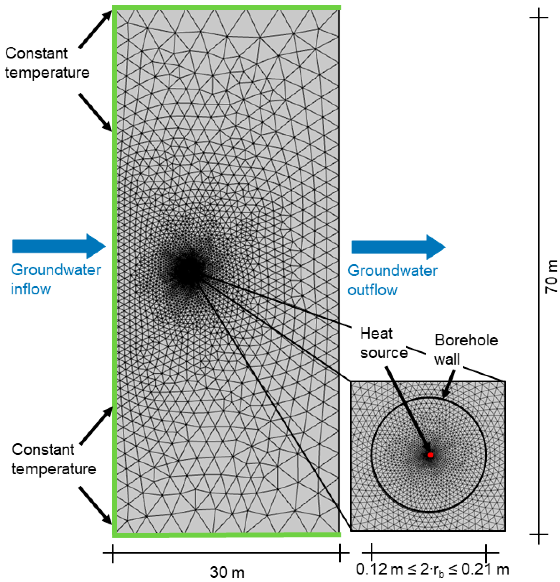
2.3. Numerical Model

In order to examine the applicability of the analytical infinite MLS solution for the temperature calculation at the borehole wall of grouted BHEs, a finite element-based numerical model considering all relevant heat transfer processes in the subsurface caused by a grouted BHE is developed in COMSOL Multiphysics^® [45]. Equivalent to the assumptions of the analytical model, a two-dimensional numerical model is set up, similar to that of Lazzari et al. [46]. In this way, the focus is set on the role of the grout, while keeping calculation time low. The error caused by ignoring the three-dimensional effects of a finite borehole is subsequently evaluated by comparison with the finite MLS (Equation (11)).

The numerical model accounts for the coupled conductive and advective heat transport in a uniform porous subsurface. The porous medium is simulated, assuming a local thermal equilibrium of the fluid and the porous matrix, with volume-averaged properties of both phases, based on Equation (1) [47]. The groundwater flow is modeled by Darcy´s law, assuming a uniform flow field with the pressure gradient as the driving force in the hydraulic potential field. Combining the heat transfer in the porous media interface with Darcy´s law interface warrants the common approach of a homogenization of the porous and fluid medium into one representative medium, i.e., no detailed model on pore-scale is necessary [48]. This requires that homogenization is feasible and that local effects of hydraulic parameter heterogeneity describing the ambient ground conditions can be ignored.

A grouted borehole with radius r_b and a centered heat source in the grouting material is embedded in the simulated ground and is treated independently, particularly with regard to heat transfer processes and its boundary conditions towards the subsurface. Since the grouting of boreholes is applied to seal the borehole against the adjacent subsurface, the grouting material is modeled using heat conduction only, so that no groundwater flow occurs within the borehole itself. The model allows for different thermal properties of the grouting material in the borehole and the porous medium around the borehole. As is common in related works (e.g., [13]), the heat exchanger pipes are not modeled explicitly but represented by a concentric heat source in the grouted borehole.

For the purpose of examining the thermal borehole resistance model for BHEs with groundwater advection, the numerical model is slightly modified. The point heat source is replaced by a centered hole in the grouting material. This simplified geometry represents a coaxial BHE or the equivalent radius for a U-tube or double-U-tube [49]. The simplification of replacing the (double-)U-tube by an equivalent radius is common practice in the analytical modeling of BHEs, especially for short-time analysis [50,51,52,53,54]. Lamarche et al. [55] have shown that the results between an analytical model with equivalent radius and a detailed numerical model are in favorable agreement.

To test a broad spectrum of conditions, a parameter study consisting of 6336 model runs is conducted, with varying subsurface and grouting material properties.

Table 1. Examined parameter ranges for the comparison between the numerical model and the infinite MLS.

Parameter Description	Unit	Value Range
Darcy velocity υDarcy	cm/day	2.94	up to		881.28
Thermal conductivity of the solid phase λs	W/(m∙K)	1.0	2.0	3.0	4.0
Porosity of the subsurface Φ	-	0.1	0.3	0.5
Thermal conductivity of the grouting material λgrout	W/(m∙K)	1.0	2.0
Borehole radius rb	m	0.06	0.075	0.09	0.105
Resulting Péclet numbers Pe	-	0.1	up to		10
Initial and boundary temperature ${\vartheta }_{E,0}$	°C	10
heat extraction rate $\dot{q}$	W/m	−20

shows all examined parameter values and ranges, covering Darcy velocities from 2.94 cm/day up to 8.81 m/day. This range corresponds to the velocities investigated in related work [29,34,40,45]. A preparatory sensitivity analysis was conducted to define the necessary numerical simulation domain and grid geometry. As a result, a suitable domain of 70 m × 30 m was determined, along with a borehole at a 10 m distance of the groundwater inflow (see Figure 2). A triangulated mesh containing 12,730 elements (Figure 2) was generated with the highest resolution in the immediate vicinity of the heat source/sink (in the BHE). The mesh increases uniformly towards the borehole wall and continues to increase in the subsurface while the temperature gradient declines. The thermal boundaries are set at a constant temperature, identical to a given initial temperature, except for the downstream boundary with an outflow condition implemented to compute the temperatures here for each simulated scenario [45]. Given this model setup with an identical setting and a homogeneous, porous subsurface with no grouting, numerically derived g-function values were compared with infinite MLS results. Relative discrepancies for the simulations with the parameter value ranges given in Table 1 were found to be less than 3%, with an absolute deviation of less than 0.01 K and a standard deviation of 0.00084 K.

2.4. Correction of Infinite MLS and Application to BHE Design

As revealed by Wagner et al., Van de Ven et al. and Wagner et al. [40,56,57], there is a deviation between the real temperature change at the wall of a grouted borehole and the corresponding temperature change calculated with the infinite MLS model. This deviation is ascribed to the different thermal and hydraulic properties of the grouting material and the subsurface. Since the operating temperature is often the limiting parameter for the dimensioning of BHEs, it is crucial to attain the correct temperature change of the BHE in the design process. Therefore, the aim of this paper is to overcome the addressed deviation by introducing a generally valid correction function $f_{cor}$ which allows for the adjustment of the infinite MLS model. This follows the same idea as the correction factor presented by Wagner et al. [40] for relating the effective Darcy velocity derived from a thermal response test to the “true” Darcy velocity in the surrounding ground.

The deviation between the numerical model with grouting and the analytical model without grouting is taken as correction in order to make the analytical model applicable for a grouted borehole. Consequently, the correction function here is defined as the ratio of the g-function of the grouted borehole as determined by the numerical model and of the g-function resulting from the infinite MLS:

$$f_{cor}=\frac{g_{GW, End,num}}{g_{GW,End, IMLS}}$$

(13)

The values or correlations that define $f_{cor}$ are deduced by comparison with the numerical model. Knowing $f_{cor}$, the mean undisturbed subsurface temperature ${\overline{\vartheta }}_{E,0}$, as well as the borehole resistance $R_b$, the mean fluid temperature in a borehole ${\overline{\vartheta }}_{BHE,End}$ at steady-state conditions can then be calculated using Equations (9) and (13) as follows:

$${\overline{\vartheta }}_{b,End}={\overline{\vartheta }}_{E,0}+\dot{q}\left(\frac{f_{cor} g_{GW,End,IMLS}}{2 \pi {\lambda }_{eff}}+R_b\right)$$

(14)

A prerequisite for the presented method is that the Darcy velocity and the thermal conductivity of the subsurface are known. These can be determined by laboratory testing of material properties or by using a thermal response test and the method found by Wagner et al. [40]. Furthermore, an average Darcy velocity can be estimated with the use of hydrogeological maps, site-specific pumping or tracer tests.

3. Results and Discussion

3.1. Compatibility of the Thermal Borehole Resistance Model for BHEs with Groundwater Advection

To implement the infinite MLS model in design programs, it has to be assessed if the non-radial temperature distribution at the borehole wall can be averaged and then be used to determine the borehole resistance for BHEs under the influence of advection. Therefore, a steady-state simulation with groundwater flow and a 48-hour transient simulation without groundwater flow are conducted, and the numerical results are compared with the analytical solution of heat conduction in an annulus. The BHE is considered to be perfectly sealed for horizontal groundwater advection in the surrounding subsurface so that only heat conduction occurs within the grouting material of the borehole. The temperature distribution around the borehole depends on groundwater flow velocity and direction and thus the computed borehole resistance differs depending on the observed angle. However, averaged over the borehole wall, the value of the thermal resistance is the same as without groundwater flow. An excerpt of the results is shown in

Table 2. Comparison of thermal borehole resistance calculations by numerical and analytical models.

Borehole Radius rb	Thermal Conductivity of the Grout λgrout	Darcy Velocity υDarcy	Numerical Simulation with Advection	Numerical Simulation without Advection		Analytical Solution
			Thermal Borehole Resistance Rb	Thermal Borehole Resistance Rb	Percentage Deviation	Thermal Borehole Resistance Rb	Percentage Deviation
m	W/(m·K)	m/s	(m·K)/W	(m·K)/W	%	(m·K)/W	%
0.060	1.0	3.40 × 10−6	0.2102	0.2096	−0.26%	0.2104	0.09%
	2.0	3.40 × 10−6	0.1051	0.1048	−0.26%	0.1052	0.09%
	1.0	1.70 × 10−5	0.2102	0.2096	−0.26%	0.2104	0.09%
	2.0	1.70 × 10−5	0.1051	0.1048	−0.26%	0.1052	0.09%
	1.0	3.40 × 10−5	0.2102	0.2096	−0.26%	0.2104	0.09%
	2.0	3.40 × 10−5	0.1051	0.1048	−0.26%	0.1052	0.09%
	1.0	1.70 × 10−4	0.2102	0.2096	−0.26%	0.2104	0.09%
	2.0	1.70 × 10−4	0.1051	0.1048	−0.26%	0.1052	0.09%
0.105	1.0	3.40 × 10−6	0.2991	0.2973	−0.61%	0.2994	0.10%
	2.0	3.40 × 10−6	0.1496	0.1487	−0.59%	0.1497	0.10%
	1.0	1.70 × 10−5	0.2991	0.2973	−0.61%	0.2994	0.10%
	2.0	1.70 × 10−5	0.1496	0.1487	−0.59%	0.1497	0.10%
	1.0	3.40 × 10−5	0.2991	0.2973	−0.61%	0.2994	0.10%
	2.0	3.40 × 10−5	0.1496	0.1487	−0.59%	0.1497	0.10%
	1.0	1.70 × 10−4	0.2991	0.2973	−0.61%	0.2994	0.10%
	2.0	1.70 × 10−4	0.1496	0.1487	−0.59%	0.1497	0.10%

. The maximum deviation between the thermal borehole resistances is less than 1% and can be ascribed to the accuracy of the numerical solution. Hence, it can be concluded that the multipole method for the determination of the thermal borehole resistances is also applicable to BHEs with groundwater advection. However, it is a prerequisite that the correct temperature at the borehole wall is calculated.

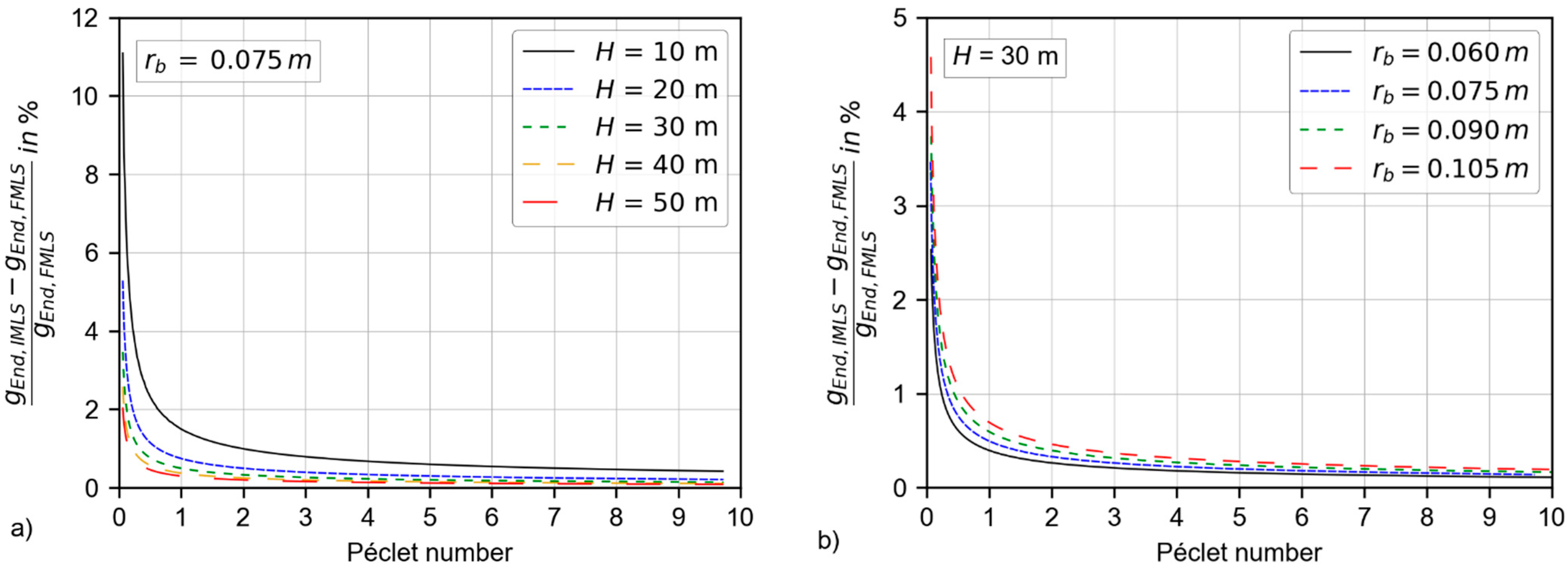
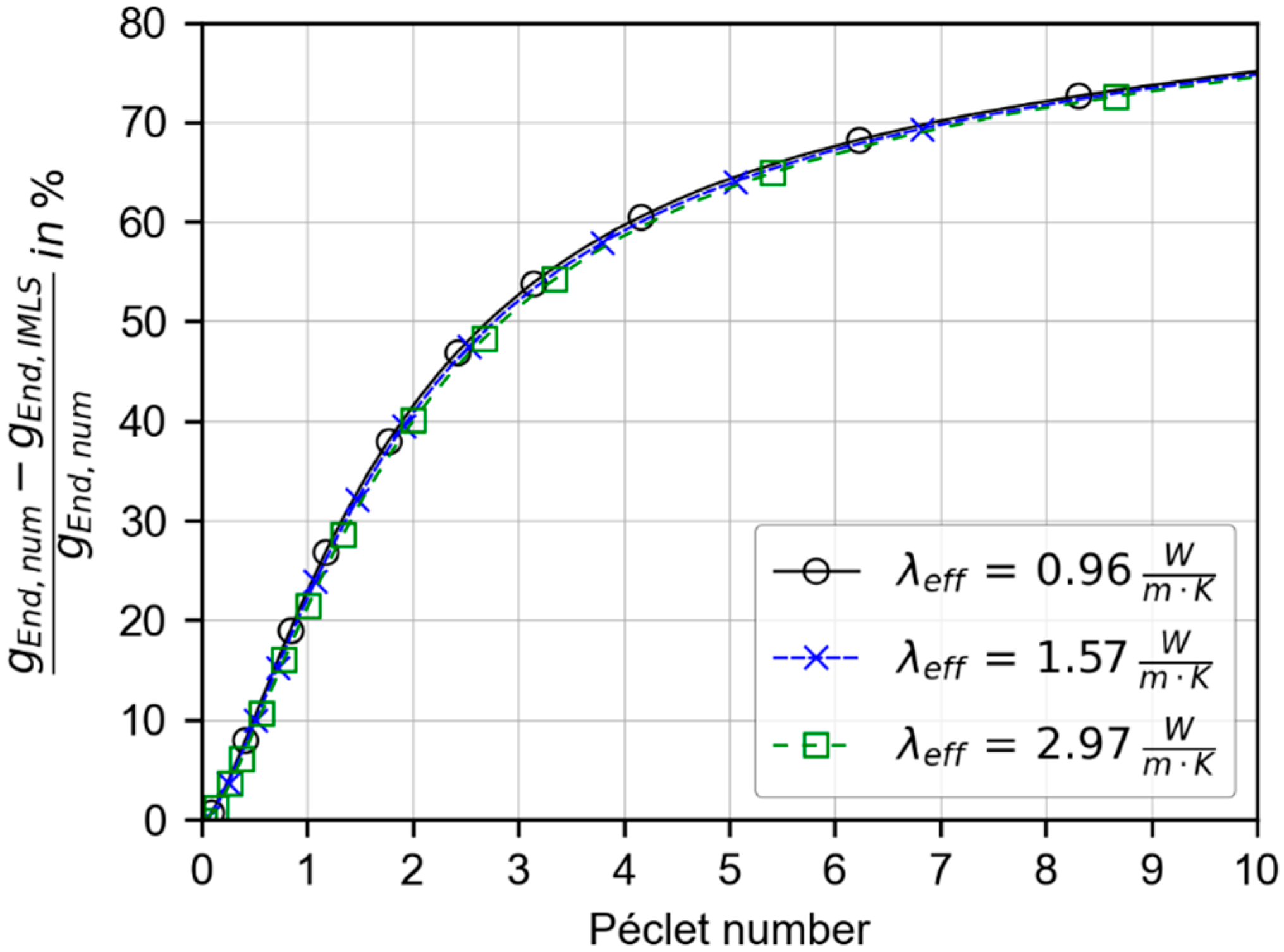
3.2. Applicability of the Infinite MLS Model to Finite Boreholes

The inaccuracy caused by using the infinite MLS instead of the finite MLS and, thus, by neglecting the three-dimensional effects at the surface and bottom of a finite BHE, is investigated by comparing both models for a broad range of parameters. Since the error between the infinite MLS and the finite MLS decreases with borehole length, only small borehole depths from 10 m up to 50 m are examined for all parameter value combinations given in Table 1.

The percentage deviation of the g-functions of the infinite MLS and the finite MLS with an isothermal boundary condition at the Earth´s surface is calculated according to Equation (15) and exemplarily depicted in Figure 3a) for a borehole radius of 0.075 m and in Figure 3b) for a borehole depth of 30 m.

$$\frac{g_{GW,End,IMLS}-g_{GW,End,FMLS}}{g_{GW,End,FMLS}}$$

(15)

As expected, the deviation between both models declines with increasing borehole depth and Péclet numbers as well as with decreasing borehole radius. For boreholes with a length of 30 m or more, the deviation is less than 5% for Pe ≥ 0.06. This reveals that a small error is introduced by neglecting the three-dimensional effects at the top and the bottom of a BHE that is influenced by horizontal groundwater flow.

Molina-Giraldo et al. [32] investigated the three-dimensional effects of a BHE with advection as well, but the Péclet number is expressed by setting the characteristic length to the borehole length (H = 50 m) (i.e., replacing r_b by H in Equation (5)). Translating the findings of Molina-Giraldo et al. [32] for a BHE with a length of 50 m, the discrepancy between the finite and the infinite MLS becomes irrelevant for Pe ≥ 0.015. The investigated range here does not cover such small Péclet numbers as by Molina-Giraldo [32], but the results are consistent. Furthermore, the infinite MLS model calculates (slightly) larger g-functions and, as a result, a greater temperature change than the finite MLS model. Hence, the infinite MLS model is the more conservative model and therefore favorable for designing BHEs of 30 m and more.

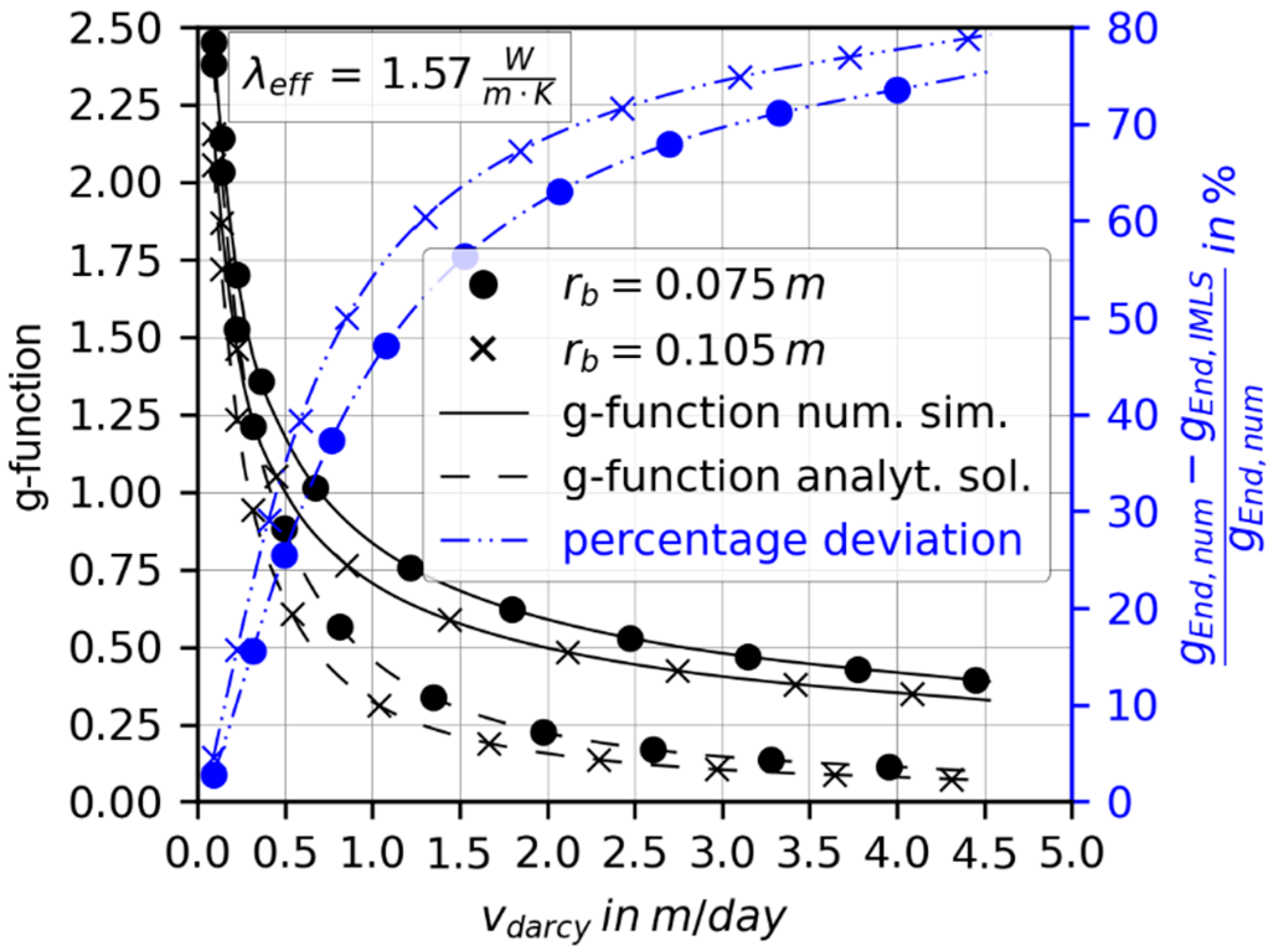
3.3. Steady-State Thermal Conditions at the Wall of a Grouted Borehole

To characterize the deviation between the numerical and analytical infinite MLS solution, the steady-state thermal conditions at the outside wall of a grouted borehole are investigated. The computed discrepancy for different borehole radii depending on the Darcy velocity is shown in Figure 4. The relative error between the g-function of the analytical solution and the numerical simulation is calculated according to:

$$\frac{g_{GW,End,num}-g_{GW,End,IMLS}}{g_{GW,End,num}}$$

(16)

It is revealed that the error gradually increases with increasing Darcy velocities. This is mainly caused by the rapidly sinking g-function values with increasing Darcy velocity. The derived curves for different radii are not identical but have a similar shape.

Investigating the deviation between both models depending on the effective thermal conductivity ${\lambda }_{eff}$ of the subsurface and the Darcy velocity $v_{Darcy}$, shows that the discrepancy decreases with higher values of ${\lambda }_{eff}$ and lower values of $v_{Darcy}$, as depicted in Figure 5. Both parameters have an effect of the same order of magnitude but in opposite directions, which means that, for example, the effect of an increased thermal conductivity can be compensated by a corresponding increase in Darcy velocity. Thus, the fraction, i.e., the relative role, of Darcy velocity (advection) and thermal conductivity (diffusion) is crucial. The relative role of advection and diffusion is expressed by the Péclet number according to Equation (5), which also includes the borehole radius as a length scale. Therefore, the combined effect of advection and diffusion for assessing the accuracy of the analytical model can be summarized in Figure 6, which confirms the rising deviation of the g-functions for a higher Péclet number. A high effective thermal conductivity ${\lambda }_{eff}$ requires a greater Darcy velocity to reach the same Péclet number in comparison to lower ${\lambda }_{eff}$. However, this barely influences the deviation of the infinite MLS, as shown in Figure 6. Thus, it can be concluded that the higher the overall influence of advection, the greater the error.

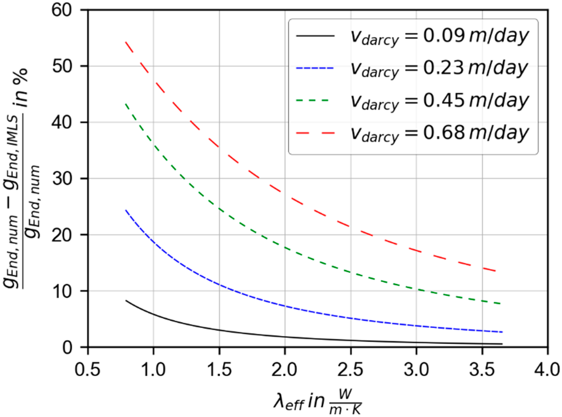
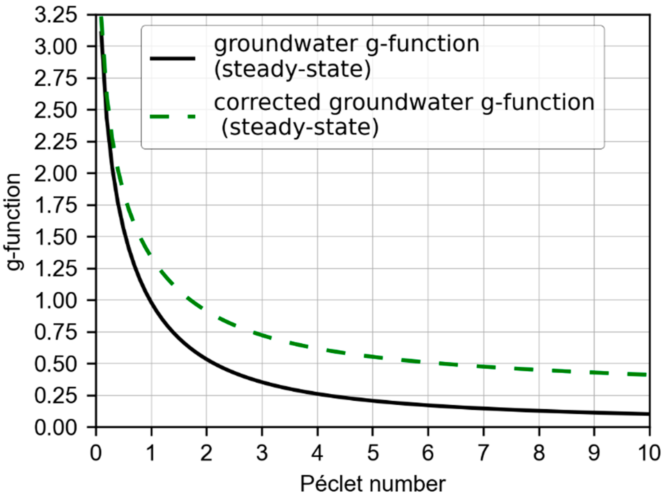
3.4. Correction Function

By introducing a correction function for the groundwater g-function for steady-state conditions, the temperature change at the borehole wall of a grouted borehole can be determined. Therefore, the results of the analytical and numerical solutions are related by Equation (13) and fitted by a second-degree polynomial as shown in Figure 7. The corrected g-function depicted in Figure 8 is generated by multiplying the correction function with the groundwater g-function and can then be implemented in design programs such as EED or GEO-HAND^light for the planning of BHEs with groundwater advection, without changing further calculation methods and without the need for a complex numerical simulation. The correction function overcomes the deficiency of neglecting the effect of the non-permeable, grouted borehole, and thus prevents a temperature change prediction that is too low during the design phase.

Since the groundwater g-function for one borehole (Equation (9)), as well as the model discrepancies, depend chiefly on the Péclet number; Figure 7 shows the correlation of the required correction based on this parameter. By means of regression analysis, a manageable, second-degree polynomial shown in Equation (17) is fitted to the simulation results, yielding a coefficient of determination of $R^2=0.993$. The second-degree polynomial is acceptable for practical applications and everyday use, since many uncertainties of a similar order of magnitude are involved while characterizing a BHE with groundwater advection. Equation (17) is only valid for Péclet numbers from Pe = 0 up to Pe = 10.

$$f_{cor}\left(Pe\right)=-6.11\cdot {10}^{-3}\cdot P{e}^2+3.68\cdot {10}^{-1}\cdot Pe+1$$

(17)

$$\mathrm{for}0\le \mathit{Pe}\le 10$$

Using a fifth-degree polynomial yields a more correct correlation reproducing the characteristic course of the simulated data. Since other parameters lead to higher uncertainties while determining the temperature of a vertical grouted borehole, a second-degree polynomial is considered adequate for practical usage.

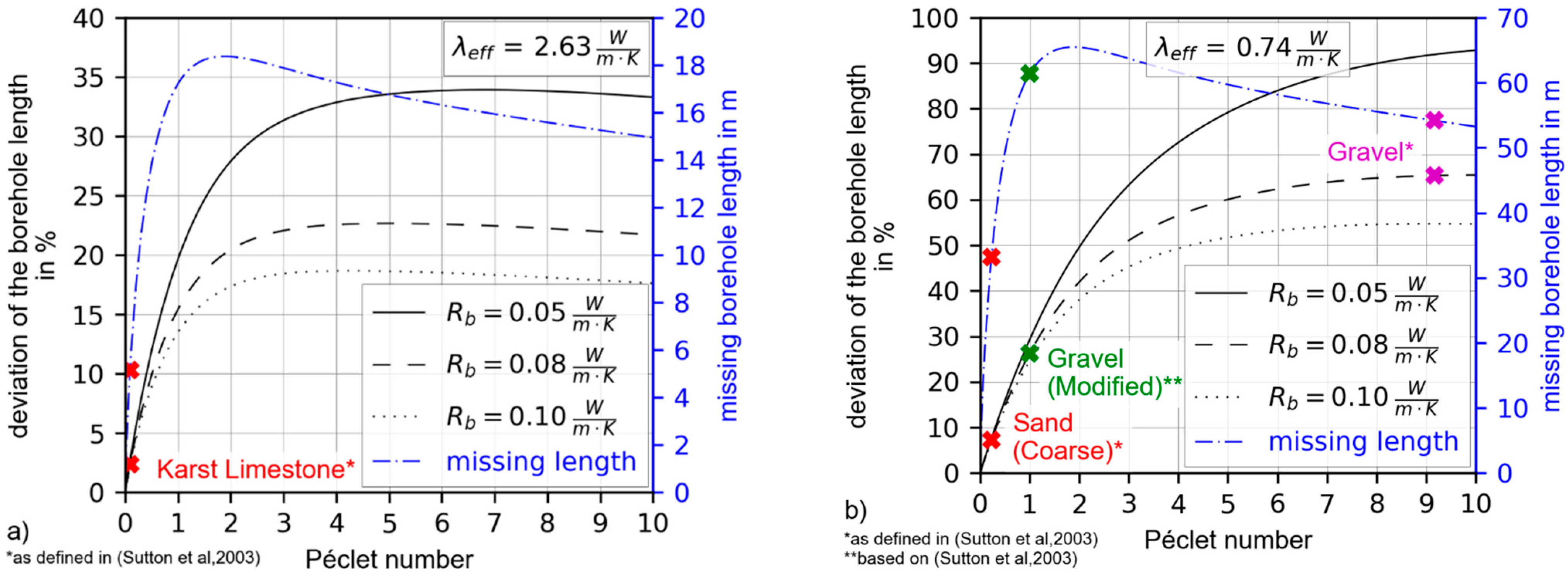
3.5. Demonstration Example

To demonstrate the impact of the proposed correction procedure for the design of a BHE, three examples for typical thermal and hydraulic property data for various geological materials as given by Sutton et al. [34] are investigated. These are listed in

Table 3. Thermal and hydraulic properties of the subsurface used for the setup of demonstration examples [34].

Material	Thermal Conductivity λ	Vol. Heat Capacity cv	Porosity Φ	Darcy Velocity υDarcy	Borehole Radius rb	Péclet Number Pe
	W/(m∙K)	MJ/(m3∙K)	-	m/yr		-
Groundwater *	0.60	4.18
Karst limestone *	3.40	13.40	0.275	31.63	0.054	0.09
Sand (coarse) *	0.8	1.40	0.385	23.14	0.054	0.23
Gravel *	0.8	1.40	0.310	945.50	0.054	9.17
Gravel (modified) **	0.8	1.40	0.310	74.25	0.075	1.00

* as defined in (Sutton et al. 2003), ** based on (Sutton et al. 2003).

as ‘Karst Limestone’, ‘Sand (Coarse)’, and ‘Gravel’. A fourth example, ‘Gravel (Modified)’, is also based on the same source but for an increased borehole radius of 0.075 m and a decreased velocity leading to a Péclet number of 1. The Péclet numbers are calculated according to Equation (5), as by Sutton et al. [34].

Considering that in this study the infinite MLS model is corrected for the effect of a grouted borehole only at steady-state conditions, an application with an almost constant heating or cooling demand is best suited. A typical example with a more or less constant cooling load is a colocation center, which releases nearly the same amount of heat all year long. The servers of the University of Applied Sciences are used in an exemplary manner for the calculation and have a constant power consumption of 8 kW of the uninterrupted power supply (UPS), as taken from measurement data of 2017 and depicted in Figure 9. The measurement data is available in the (see supplementary material Table S1: Cooling load of the servers at Biberach University of Applied Sciences).

The power consumption of the UPS is equivalent to the required cooling load of the colocation center. The mean undisturbed subsurface temperature next to the colocation center is assumed to be about 12 °C. A maximum temperature increase of the mean fluid temperature of 10 K is desired in order to guarantee a mean fluid temperature of 22 °C, which is necessary to operate the cooling device of the colocation center.

Using the thermal and hydraulic properties listed in Table 3, a heat injection rate of 8 kW, a thermal resistance of 0.08 (m^∙K)/W, an undisturbed subsurface temperature of 12 °C, and a maximum temperature increase of 10 K, the required borehole depths and the resulting specific heat injection rates are determined by transforming Equation (14). Furthermore, the percentage deviation of the aforementioned properties calculated with and without the proposed correction in Equation (17) are listed as well. The percentage deviation expresses the discrepancy between both calculations compared with the calculation using the uncorrected g-function.

The calculation examples in

Table 4. Calculation example for the four cases listed in Table 3.

Heat Injection Rate						8.00	kW
Borehole Resistance						0.08	(m·K)/W
Maximum Temperature Change of the Subsurface						10	K
	Péclet Number	Model Selection	g- Function	Borehole Length	Percentage Deviation of the Borehole Length	Specific Heat Injection Rate	Percentage Deviation of the Heat Injection Rate
	-	-	-	m	%	W/m	%
Karst limestone *	0.09	FLS	6.6	383.52	74.39%	20.86	42.66%
		IMLS without correction	3.22	219.93	0.00%	36.38	0.00%
		IMLS with correction	3.32	224.60	2.13%	35.62	2.08%
Sand (coarse) *	0.23	FLS	6.6	1226.29	161.34%	6.52	61.74%
		IMLS without correction	2.30	469.24	0.00%	17.05	0.00%
		IMLS with correction	2.49	501.66	6.91%	15.95	6.46%
Gravel *	9.17	FLS	6.6	1202.67	1350.07%	6.65	93.10%
		IMLS without correction	0.11	82.94	0.00%	96.46	0.00%
		IMLS with correction	0.42	137.10	65.31%	58.35	39.51%
Gravel (modified) **	1.00	FLS	6.6	1202.67	414.82%	6.65	80.58%
		IMLS without correction	0.98	233.61	0.00%	34.25	0.00%
		IMLS with correction	1.34	2954.67	26.14%	27.15	20.72%

* as defined in (Sutton et al. 2003), ** based on (Sutton et al. 2003).

show that considering groundwater flow leads a shorter borehole required for a given heat demand, i.e., using the MLS model instead of the finite line source (FLS) model is strongly recommended if advection is present. However, for rising Péclet numbers, the borehole depth is increasingly underestimated and thus the specific heat extraction rate is overestimated for grouted boreholes if the MLS solution is not corrected. For a constant effective thermal conductivity but a rising Péclet number, i.e., rising contribution by groundwater flow and thus higher Darcy velocity, the percentage deviation, as well as the absolute deviation, increases rapidly for small Péclet numbers. In the range of Pe = 0 to 10, the absolute deviation reaches a maximum around Pe = 2 for the investigated examples and then slowly decreases (Figure 10). The wrong estimation without correction can also be quantified by missing borehole length. For equal borehole radii, the percentage deviation of the borehole length varies with the borehole resistance, since a greater resistance and thus a worse thermal conductivity of the grouting material leads to a larger overall borehole length. The absolute missing borehole length caused by ignoring the grouted and sealed borehole is, on the contrary, independent of the borehole resistance. The percentage deviation and the missing borehole length for the four demonstration examples are explicitly marked in Figure 10.

4. Conclusions

This paper assesses the suitability of the analytical infinite MLS model for the dimensioning of vertical finite and grouted BHEs with horizontal groundwater advection for steady-state conditions. Therefore, the relevant aspects for the analytically based determination of the operating temperature of BHEs are investigated concerning the use of the infinite MLS model.

The initial step was the investigation of the applicability of established thermal borehole resistance models for BHEs under purely conductive conditions concerning groundwater advection. Due to the non-radially symmetric temperature distribution around the borehole, the suitability of the mean borehole temperature for the determination of the borehole resistance is investigated. It is found that established analytical methods to determine the borehole thermal resistance as a mean value over the borehole radius can also be applied to BHEs with groundwater advection.

In the second phase, the applicability of the infinite MLS model to boreholes of finite length is evaluated by comparing the g-functions resulting from the infinite and the finite MLS. For a finite MLS with an isothermal boundary condition, the deviation is less than 5% for BHEs of a depth of 30 m or more, and for Péclet numbers greater than 0.05. Here, the use of the infinite MLS leads to only slightly larger g-function values and temperature changes at the borehole wall than the more realistic finite MLS model.

The major discrepancy when applying the infinite MLS model to finite, grouted BHEs is due to the grouting of the borehole, since the grouting is almost impermeable for groundwater flow, while the infinite MLS model represents a homogeneous groundwater flow (also within the borehole region). This discrepancy is investigated by comparing the infinite MLS model with numerical simulations in an extensive parameter study. The deviation could be traced back to one main parameter the Péclet number. Using the Péclet number, a correction function is introduced to overcome the discrepancy of the infinite MLS model. The described correction procedure allows for a more precise estimation of the temperature change at the borehole wall for steady-state conditions. A calculation of the BHE operating temperature that is too optimistic is thereby avoided, which is necessary to ensure operational safety. It is shown that, depending on the Péclet number, the use of the infinite MLS model without correction will lead to an underestimation of the required borehole length.

With the correction function found in this study, the infinite MLS model, together with established borehole resistance models, has been found to be well-suited for the dimensioning of finite, vertical, and grouted boreholes in the presence of groundwater advection for steady-state conditions, boreholes of at least 30 m in length, and Péclet numbers from 0.05 on. Since the developed correction function is valid for single boreholes and steady-state conditions only, further development will focus on transient conditions and borehole fields.

References

1. Blum, P.; Campillo, G.; Münch, W.; Kölbel, T. CO2 savings of ground source heat pump systems—A regional analysis. Renew. Energy 2010, 35, 122–127. [Google Scholar] [CrossRef]
2. Bayer, P.; Saner, D.; Bolay, S.; Rybach, L.; Blum, P. Greenhouse gas emission savings of ground source heat pump systems in Europe: A review. Renew. Sustain. Energy Rev. 2012, 16, 1256–1267. [Google Scholar] [CrossRef]
3. Aditya, G.R.; Narsilio, G.A. Environmental assessment of hybrid ground source heat pump systems. Geothermics 2020, 87, 101868. [Google Scholar] [CrossRef]
4. Rees, S.J. An introduction to ground-source heat pump technology. In Advances in Ground-Source Heat Pump Systems; Rees, S., Ed.; Elsevier Reference Monographs; Elsevier: Amsterdam, The Netherlands, 2016; pp. 1–25. [Google Scholar]
5. Yu, X.; Zhang, Y.; Deng, N.; Wang, J.; Zhang, D.; Wang, J. Thermal response test and numerical analysis based on two models for ground-source heat pump system. Energy Build. 2013, 66, 657–666. [Google Scholar] [CrossRef]
6. Saner, D.; Juraske, R.; Kübert, M.; Blum, P.; Hellweg, S.; Bayer, P. Is it only CO2 that matters? A life cycle perspective on shallow geothermal systems. Renew. Sustain. Energy Rev. 2010, 14, 1798–1813. [Google Scholar] [CrossRef]
7. Diao, N.; Li, Q.; Fang, Z. Heat transfer in ground heat exchangers with groundwater advection. Int. J. Therm. Sci. 2004, 43, 1203–1211. [Google Scholar] [CrossRef]
8. Ingenieure, V.D. Thermische Nutzung des Untergrunds: Erdgekoppelte Wärmepumpenanlagen; Beuth Verlag GmbH: Berlin, Germany, 2019. [Google Scholar]
9. Reuss, M.; Karrer, H.; Gehlin, S.; Andersson, O.; Bjorn, H.; Nagano, K.; Katsura, T.; Metzner, M. IEA ECES ANNEX 27: Quality Management in Design, Construction and Operation of Borehole Systems. Final Report. 2020. Available online: https://iea-eces.org/wp-content/uploads/public/IEA-ECES-ANNEX-27-Final-Report-20201118.pdf (accessed on 7 December 2020).
10. Rivera, J.A.; Blum, P.; Bayer, P. Increased ground temperatures in urban areas: Estimation of the technical geothermal potential. Renew. Energy 2017, 103, 388–400. [Google Scholar] [CrossRef] [Green Version]
11. FascÌ, M.L.; Lazzarotto, A.; Acuna, J.; Claesson, J. Analysis of the thermal interference between ground source heat pump systems in dense neighborhoods. Sci. Technol. Built Environ. 2019, 25, 1069–1080. [Google Scholar] [CrossRef] [Green Version]
12. EED Version 4—Earth Energy Designer: Update Manual. 2020. Available online: https://www.buildingphysics.com/manuals/EED4.pdf (accessed on 1 March 2021).
13. Spitler, J.D.; Marshall, C.L.; Manickam, A.; Dharapuram, M.; Delahoussaye, R.D.; Yeung, K.W.D.; Young, R.; Bhargava, M.; Mokashi, S.; Yavuzturk, C.; et al. GLHEPro 5.0 For Windows: Users’ Guide. 2016. Available online: https://hvac.okstate.edu/sites/default/files/pubs/glhepro/GLHEPRO_5.0_Manual.pdf (accessed on 1 March 2021).
14. Huber, A. Bedienungsanleitung zum Programm EWS; Huber Energietechnik AG: Zürich, Switzerland, 2016. [Google Scholar]
15. Koenigsdorff, R. Oberflächennahe Geothermie für Gebäude: Grundlagen und Anwendungen Zukunftsfähiger Heizung und Kühlung; Fraunhofer IRB-Verl.: Stuttgart, Germany, 2011. [Google Scholar]
16. Erol, S.; François, B. Multilayer analytical model for vertical ground heat exchanger with groundwater flow. Geothermics 2018, 71, 294–305. [Google Scholar] [CrossRef]
17. De Carli, M.; Tonon, M.; Zarrella, A.; Zecchin, R. A computational capacity resistance model (CaRM) for vertical ground-coupled heat exchangers. Renew. Energy 2010, 35, 1537–1550. [Google Scholar] [CrossRef]
18. Bennet, J.; Claesson, J.; Hellström, G. Multipole Method to Compute the Conductive Heat Flows to and Between Pipes in a Composite Cylinder; Notes on Heat Transfer; University of Lund: Lund, Sweden, 1987. [Google Scholar]
19. Javed, S.; Spitler, J.D. Calculation of Borehole Thermal Resistance; Elsevier: Amsterdam, The Netherlands, 2016. [Google Scholar] [CrossRef]
20. Claesson, J.; Hellström, G. Multipole method to calculate borehole thermal resistances in a borehole heat exchanger. HVAC&R Res. 2011, 17, 895–911. [Google Scholar] [CrossRef]
21. Eskilson, P. Thermal Analysis of Heat Extraction. Boreholes. Dissertation, University of Lund, Lund, Sweden, 1987. [Google Scholar]
22. Javed, S.; Fahlén, P.; Claesson, J. Vertical ground heat exchangers: A review of heat flow models. In Proceedings of the Effstock 2009, Stockholm, Sweden, 14–17 June 2009. [Google Scholar]
23. Zeng, H.Y.; Diao, N.R.; Fang, Z.H. A finite line-source model for boreholes in geothermal heat exchangers. Heat Trans. Asian Res. 2002, 31, 558–567. [Google Scholar] [CrossRef]
24. Angelotti, A.; Ly, F.; Zille, A. On the applicability of the moving line source theory to thermal response test under groundwater flow: Considerations from real case studies. Geotherm Energy 2018, 6, 12. [Google Scholar] [CrossRef] [Green Version]
25. Antelmi, M.; Alberti, L.; Angelotti, A.; Curnis, S.; Zille, A.; Colombo, L. Thermal and hydrogeological aquifers characterization by coupling depth-resolved thermal response test with moving line source analysis. Energy Convers. Manag. 2020, 225, 113400. [Google Scholar] [CrossRef]
26. Chiasson, A.; O´Connell, A. New analytical solution for sizing vertical borehole ground heat exchangers in environments with significant groundwater flow: Parameter estimation from thermal response test data. HVAC&R Res. 2011, 17, 1000–1011. [Google Scholar] [CrossRef]
27. Claesson, J.; Hellström, G. Analytical Studies of the Influence of Regional Groundwater Flow on the Performance of Borehole Heat Exchangers. In Proceeding of the 8th International Conference on Thermal Energy Storage, Stuttgart, Germany, 20 August 2000. [Google Scholar]
28. Hecht-Méndez, J.; de Paly, M.; Beck, M.; Bayer, P. Optimization of energy extraction for vertical closed-loop geothermal systems considering groundwater flow. Energy Convers. Manag. 2013, 66, 1–10. [Google Scholar] [CrossRef]
29. Katsura, T.; Nagano, K.; Takeda, S.; Shimakura, K. Heat Transfer Experiment in the Ground with Ground Water Advection. In Proceeding of the 10th International Conference on Thermal Energy Storage, Galloway, New Jersey, USA, 31 May–2 June 2006. [Google Scholar]
30. Kölbel, T. Grundwassereinfluss auf Erdwärmesonden: Geländeuntersuchungen und Modellrechnungen. Ph.D. Thesis, Karlsruher Institut für Technologie, Karlsruhe, Germany, 2010. [Google Scholar]
31. Mohammadzadeh Bina, S.; Fujii, H.; Kosukegawa, H.; Farabi-Asl, H. Evaluation of ground source heat pump system’s enhancement by extracting groundwater and making artificial groundwater velocity. Energy Convers. Manag. 2020, 223, 113298. [Google Scholar] [CrossRef]
32. Molina-Giraldo, N.; Blum, P.; Zhu, K.; Bayer, P.; Fang, Z. A moving finite line source model to simulate borehole heat exchangers with groundwater advection. Int. J. Therm. Sci. 2011, 50, 2506–2513. [Google Scholar] [CrossRef]
33. Stauffer, F.; Bayer, P.; Blum, P.; Molina Giraldo, N.A.; Kinzelbach, W. Thermal Use of Shallow Groundwater; First issued in paperback 2017; Environmental engineering; CRC Press, Taylor & Francis Group: Boca Raton, FL, USA, 2017. [Google Scholar]
34. Sutton, M.G.; Nutter, D.W.; Couvillion, R.J. A Ground Resistance for Vertical Bore Heat Exchangers With Groundwater Flow. J. Energy Resour. Technol. 2003, 125, 183–189. [Google Scholar] [CrossRef]
35. Zhang, L.; Shi, Z.; Yuan, T. Study on the Coupled Heat Transfer Model Based on Groundwater Advection and Axial Heat Conduction for the Double U-Tube Vertical Borehole Heat Exchanger. Sustainability 2020, 12, 7345. [Google Scholar] [CrossRef]
36. Tye-Gingras, M.; Gosselin, L. Generic ground response functions for ground exchangers in the presence of groundwater flow. Renew. Energy 2014, 72, 354–366. [Google Scholar] [CrossRef]
37. Hellström, G. Ground Heat Storage: Thermal Analyses of Duct Storage Systems Theory. Ph.D. Thesis, University of Lund, Lund, Sweden, 1991. [Google Scholar]
38. Rivera, J.A.; Blum, P.; Bayer, P. Analytical simulation of groundwater flow and land surface effects on thermal plumes of borehole heat exchangers. Appl. Energy 2015, 146, 421–433. [Google Scholar] [CrossRef]
39. Guo, Y.; Hu, X.; Banks, J.; Liu, W.V. Considering buried depth in the moving finite line source model for vertical borehole heat exchangers—A new solution. Energy Build. 2020, 214, 109859. [Google Scholar] [CrossRef]
40. Wagner, V.; Blum, P.; Kübert, M.; Bayer, P. Analytical approach to groundwater-influenced thermal response tests of grouted borehole heat exchangers. Geothermics 2013, 46, 22–31. [Google Scholar] [CrossRef]
41. Carslaw, H.S.; Jaeger, J.C. Conduction of Heat in Solids, 2nd ed.; Oxford Science Publications; Clarendon Press: Oxford, UK, 1959. [Google Scholar]
42. Bear, J. Dynamics of Fluids in Porous Media; Dover Books on Physics and Chemistry; Dover: New York, NY, USA, 1988. [Google Scholar]
43. Chaudhry, M.A.; Zubair, S.M. On a Class of Incomplete Gamma Functions with Applications: Chapman and Hall/CRC; Chapman and Hall/CRC: Boca Raton, FL, USA, 2001. [Google Scholar]
44. Rivera, J.A.; Blum, P.; Bayer, P. Influence of spatially variable ground heat flux on closed-loop geothermal systems: Line source model with nonhomogeneous Cauchy-type top boundary conditions. Appl. Energy 2016, 180, 572–585. [Google Scholar] [CrossRef] [Green Version]
45. COMSOL Multiphysics, version 5.6; COMSOL AB: Stockholm, Sweden, 2020.
46. Lazzari, S.; Priarone, A.; Zanchini, E. Long-Term Performance of Borehole Heat Exchanger Fluids with Groundwater Movement: Excerpt from the Proceedings of the COMSOL Conference 2010 Paris. In Proceedings of the COMSOL Conference 2010, Paris, France, 17–19 November 2010. [Google Scholar]
47. Gossler, M.A.; Bayer, P.; Zosseder, K. Experimental investigation of thermal retardation and local thermal non-equilibrium effects on heat transport in highly permeable, porous aquifers. J. Hydrol. 2019, 578, 124097. [Google Scholar] [CrossRef]
48. 48. COMSOL Multiphysics®. Subsurface Flow Module: User´s Guide. 2021. Available online: https://doc.comsol.com/5.4/doc/com.comsol.help.ssf/SubsurfaceFlowModuleUsersGuide.pdf (accessed on 24 August 2021).
49. Claesson, J.; Dunand, A. Heat Extraction from the Ground by Horizontal Pipes: A Mathematical Analysis; Swedish Council for Building Research: Stockholm, Sweden, 1983. [Google Scholar]
50. Gu, Y.; O´Neal, D.L. Development of an Equivalent Diameter Expression for Vertical U-Tubes Used in Ground-Coupled Heat Pumps. Transactions-Am. Soc. Heat. Refrig. Air Cond. Eng. 1998, 104, 347–355. [Google Scholar]
51. Gu, Y.; O’Neal, D.L. An Analytical Solution to Transient Heat Conduction in a Composite Region with a Cylindrical Heat Source. J. Sol. Energy Eng. 1995, 242–248. [Google Scholar] [CrossRef]
52. Kavanaugh, S.P. Simulation and Experimental Verification of Vertical Ground-coupled Heat Pump Systems. Ph.D. Thesis, Oklahoma State University, Stillwater, OK, USA, 1985. [Google Scholar]
53. Lazzarotto, A.; Pallard, W.M. Thermal Response Test Performance Evaluation with Drifting Heat Rate and Noisy Measurements. In Proceedings of the European Geothermal Congress, Hague, The Netherlands, 11–14 June 2019; pp. 1–9. [Google Scholar]
54. Javed, S.; Claesson, J. New analytical and numerical solutions for the short-term analysis of vertical ground heat exchangers. ASHRAE Trans. 2011, 117, 3–12. [Google Scholar]
55. Lamarche, L.; Beauchamp, B. New solutions for the short-time analysis of geothermal vertical boreholes. Int. J. Heat Mass Transf. 2007, 50, 1408–1419. [Google Scholar] [CrossRef]
56. Van de Ven, A.; Koenigsdorff, R.; Hofmann, S. Entwicklung konsistenter Auslegungsmodelle für oberflächennahe geothermische Quellensysteme. In Proceedings of the BauSIM 2018. 7. Deutsch-Österreichische IBPSA-Konferenz, Karlsruhe, Germany, 26–28 September 2018; Karlsruher Institut für Technologie: Karlsruhe, Germany, 2018; pp. 508–515. [Google Scholar]
57. Wagner, V.; Bayer, P.; Bisch, G.; Kübert, M.; Blum, P. Hydraulic characterization of aquifers by thermal response testing: Validation by large-scale tank and field experiments. Water Resour. Res. 2014, 50, 71–85. [Google Scholar] [CrossRef]
Figure 1. Temperature distribution around a heat sink with groundwater advection.
Geosciences 11 00410 g001
Figure 2. Model domain of the numerical model and its boundary conditions.
Geosciences 11 00410 g002
Figure 3. Percentage deviation of the g-functions calculated with the infinite and finite MLS with an isothermal boundary condition at the ground surface (a) for a borehole radius of rb = 0.075 m and (b) a borehole length of H = 30 m.
Geosciences 11 00410 g003
Figure 4. Deviation of the g-functions between the numerical model with a grouted borehole and the analytical infinite MLS model.
Geosciences 11 00410 g004
Figure 5. Percentage deviation of the g-functions depending on the effective thermal conductivity for different Darcy velocities.
Geosciences 11 00410 g005
Figure 6. Percentage deviation of the g-functions depending on the Péclet number for different effective thermal conductivities.
Geosciences 11 00410 g006
Figure 7. Second-degree polynomial correction function for the infinite MLS for steady-state conditions.
Geosciences 11 00410 g007
Figure 8. Groundwater g-function values for steady state conditions with and without correction.
Geosciences 11 00410 g008
Figure 9. Cooling load of the servers at Biberach University of Applied Sciences.
Geosciences 11 00410 g009
Figure 10. Deviation in borehole length depending on the Péclet number for the thermal properties as listed in Table 3 of (a) Karst Limestone and (b) Gravel and Sand (coarse).
Geosciences 11 00410 g010