Metamodel-Based Slope Reliability Analysis—Case of Spatially Variable Soils Considering a Rotated Anisotropy

Abstract

A rotation of the anisotropic soil fabric pattern is commonly observed in natural slopes with a tilted stratification. This study investigates the rotated anisotropy effects on slope reliability considering spatially varied soils. Karhunen–Loève expansion is used to generate the random fields of the soil shear strength properties (i.e., cohesion and friction angle). The presented probabilistic analyses are based on a meta-model combining Sparse Polynomial Chaos Expansion (SPCE) and Global Sensitivity Analysis (GSA). This method allows the number of involved random variables to be reduced and then the computational efficiency to be improved. Two kinds of deterministic models, namely a discretization kinematic approach and a finite element limit analysis, are considered. A variety of valuable results (i.e., failure probability, probability density function, statistical moments of model response, and sensitivity indices of input variables) can be effectively provided. Moreover, the influences of the rotated anisotropy, autocorrelation length, coefficient of variation and cross-correlation between the cohesion and friction angle on the probabilistic analysis results are discussed. The rotation of the anisotropic soil stratification has a significant effect on the slope stability, particularly for the cases with large values of autocorrelation length, coefficient of variation, and cross-correlation coefficient.

1. Introduction

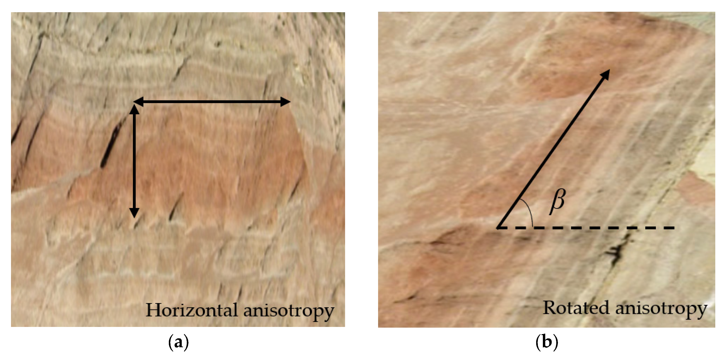
Inherent spatial variability of soil properties plays a significant role in probabilistic analyses. Random field theory has been widely used to model this feature to discuss the soil spatial variability effects on slope reliability [1,2,3,4,5]. However, these studies mainly focused on isotropic soils or soils with a horizontal stratification (Figure 1a). In practice, due to the complex deposition process, soil rotated anisotropy, as shown in Figure 1b, can also be found [6]. The stratification is inclined with the horizontal direction by a rotation angle β. Effects of the rotated anisotropy on slope stability have been investigated in the literature. Griffiths et al. [7] demonstrated that the rotated anisotropy has a very significant effect on slope failure probability and found that the failure probability is higher when the soil stratification is parallel to the slope surface. Zhu et al. [6] considered a real slope case with different fabric rotation angles and found that the stratification orientation can influence the failure mechanism. Huang et al. [8] investigated the rotated anisotropy effect on slope stability considering conditional random fields and found that different sampling patterns may lead to significantly different failure probabilities. These works provide interesting insights into the slope reliability analysis with consideration of the rotated anisotropy. However, some limitations can be identified.

Firstly, concerning the deterministic analysis, numerical analysis methods or the Limit Equilibrium Method (LEM) were performed to calculate the results. Numerical analysis methods are popular because of their accuracy and detailed visualizations. However, these methods suffer from a heavy computational burden in the procedures of numerical model construction and calculation, particularly for probabilistic analyses, which require a large number of simulations. Therefore, using analytical methods, at least in the preliminary design stage, is preferable due to the fact that it can reduce the computational burden for most cases, guaranteeing accuracy of the results. LEM [6,8] is widely used for slope stability analyses due to its simple theory and calculation procedure. 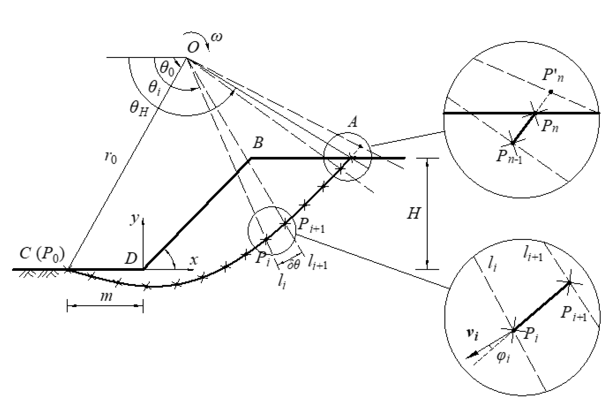However, this method considers the failure surface as a circle and makes assumptions for the inter-slice forces, which may provide biased results [9]. Limit Analysis (LA) is another commonly adopted analytical method. This method considers the plasticity theory and can lead to more rigorous results than LEM. The upper bound limit analysis (i.e., the kinematic approach), can give a rigorous upper bound solution. It is widely used compared to the lower bound limit analysis, since it is based on the kinematically admissible velocity field, which is convenient to be obtained. LA was improved by discretizing the traditional failure surface (log-spiral) into a variety of segments [10,11,12] to consider the spatial variation of soil properties. It could solve the inevitably introduced complex and tedious integral calculations of the traditional log-spiral mechanism when non-homogeneous cases are considered. This method has been used for tunnels [11], foundations [12], and slopes [10]. It is implemented in this study to effectively consider the spatial variability of soil parameters.

Moreover, in the framework of probabilistic analyses, Monte Carlo Simulations (MCSs) have been commonly employed in the existing studies to calculate the failure probability (P_f) [13,14]. This method is widespread due to its simple calculation and robustness. However, it may lead to a heavy computational burden, especially for the cases with small failure probabilities. In order to overcome this inconvenience, meta-modelling techniques were developed and aim to build fast-to-evaluate metamodels to replace the original expensive deterministic computational models [15]. These metamodels include kriging [16,17], polynomial-chaos expansions (PCEs) [18,19], and support vector machines [20,21]. Jiang et al. [2] proposed a non-intrusive stochastic finite element method for the slope reliability considering the spatially variable shear strength parameters based on the PCE method, which improves the slope probabilistic analyses. However, the number of polynomials within the PCE metamodel increases drastically with the increase of the input variables number and the PCE order. In order to further improve the calculation efficiency, the extension of polynomial-chaos expansion, namely Sparse Polynomial Chaos Expansion (SPCE), was used in the probabilistic analyses.

On the other hand, many variables (e.g., more than 100) are introduced for the random field discretization and are considered as input variables in the probabilistic analyses. This feature makes a metamodel-based probabilistic analysis difficult and takes a long time to create. In order to overcome this problem, the combination of SPCE and Global Sensitivity Analysis (GSA) is introduced in this paper for the reliability analyses. It presents a high efficiency since dimension reduction is implemented by the GSA based on a low-order SPCE model. This means that the significant input variables are selected firstly according to Sobol indices obtained by a low-order SPCE-based GSA to form the input space [22]. It is followed by a high-order SPCE construction using an active learning algorithm with a new proposed stopping condition. After that, the MCS and GSA can be employed to provide a variety of valuable results, which include failure probabilities, probability density function (PDF), statistical moments of the model response, and sensitivity indices of input variables.

This study aims to perform a probabilistic stability analysis of slopes with consideration of the soil rotated anisotropy by using the DSG–MG procedure, which includes the deterministic method discretization kinematic approach (DKA) and the probabilistic methods SPCE/GSA and MCS. After the introduction of the random field generation, the deterministic and probabilistic methods are presented in detail. Comparisons with the existing studies and some discussions based on the proposed DSG–MG procedure are then provided. The improvements and contributions of this study compared to existing studies about the slope probabilistic stability are as follows: (1) the analytical DKA can consider the soil spatial variability due to the employed discretized mechanism, which shows a good efficiency compared to numerical models; (2) the proposed DSG–MG procedure can solve effectively the high dimensional stochastic problems. It allows the computational burden of probabilistic analyses to be reduced and provides a variety of valuable results with guaranteed accuracy; (3) the influences of rotated anisotropy, autocorrelation lengths, coefficient of variation and cross-correlation of the slope stability are discussed. Some recommendations are then proposed based on the probabilistic results.

2. Random Field Generation

A random field can describe the spatial correlation of a soil property in different locations and represent nonhomogeneous characteristics. Several methods were developed for the discretization of random fields: among others, the spatial average method, the midpoint method, and the series expansion methods. Compared to the first two methods, which are sensitive to the finite element mesh size and require a large number of random variables to achieve a good field approximation, the series expansion methods (such as Karhunen–Loève (K–L) expansion and the optimal linear estimation expansion methods) are more efficient. The series expansion methods result in a Gaussian field represented by a series of random variables and deterministic spatial functions. The accuracy of the field depends on the number of terms used in the series expansion and the adopted expansion method. K–L expansion is used in this study since it requires the fewest random variables for a given accuracy and is independent of the finite element discretization [23]. This method is popular in geotechnical engineering, such as for dams [22] and tunnels [18].

2.1. Spatial Correlation

Autocorrelation length and function are used to characterize the soil properties with correlation. For a given autocorrelation function, a large autocorrelation length value implies that the soil property is highly correlated over a large spatial extent, resulting in a smooth variation within the soil profile.

A Gaussian random field can be described by its mean $\mu (x)$, variance $\sigma (x)$, and an autocorrelation function ρ. In this study, an exponential autocorrelation function that involves the rotation angle of soil anisotropy is used and reads as follows:

$$\rho =\exp (-\frac{\left|\mathsf{\Delta }x\cos \beta +\mathsf{\Delta }y\sin \beta \right|}{l_h}-\frac{\left|-\mathsf{\Delta }x\sin \beta +\mathsf{\Delta }y\cos \beta \right|}{l_v})$$

(1)

where $l_h$ and $l_v$ are, respectively, the autocorrelation distances in the horizontal and vertical directions; β is the rotation angle; and $\mathsf{\Delta }x$ and $\mathsf{\Delta }y$ are the distances between two arbitrary points in the horizontal and vertical directions, respectively.

2.2. K–L Expansion

Karhunen–Loève expansion is based on the spectral decomposition of its autocovariance function (i.e., the product of the autocorrelation function ρ and the random field variance). The realization of the random field, denoted $H(x,\xi )$, can be defined by [23,24]

$$H(x,\xi )=\mu +\sigma {\displaystyle \sum _{i=1}^{\infty }\sqrt{{\lambda }_i}{\theta }_i(x){\xi }_i}\cong \mu +\sigma {\displaystyle \sum _{i=1}^S\sqrt{{\lambda }_i}{\theta }_i(x){\xi }_i}$$

(2)

where μ and σ are, respectively, the mean value and standard deviation of the random field; ${\lambda }_i$ and ${\theta }_i$ are the eigenvalues and eigenfunctions, respectively, of the autocovariance function; ${\xi }_i$ is a set of uncorrelated random variables; and S is the size of the truncated series expansion. It should be noted that S depends on the target accuracy, autocorrelation length, and random field dimension. The value of S is determined using a criterion based on the error of the truncated series expansion, which can be obtained by

$$\epsilon =\frac{1}{\mathsf{\Omega }}{\displaystyle {\int }_{\mathsf{\Omega }}\left[1-{\displaystyle \sum _{i=1}^S{\lambda }_i{\theta }_i{}^2(x)}\right]}d\mathsf{\Omega }$$

(3)

where $\mathsf{\Omega }$ represents the validity domain of the random field.

2.3. Cross-Correlated Log-Normal Random Fields

A log-normal random field based on the K–L expansion can be expressed as [22]

$$H(x,\xi )=\exp \left[{\mu }_{\ln }+{\sigma }_{\ln }{\displaystyle \sum _{i=1}^S\sqrt{{\lambda }_i}{\theta }_i(x){\xi }_i}\right]=\exp \left[{\mu }_{\ln }+{\sigma }_{\ln }G(x,\xi )\right]$$

(4)

where $G(x,\xi )$ is a standard normally distributed random field with S terms; ${\mu }_{\ln }$ is the mean value of the log-normal random field; and ${\sigma }_{\ln }$ is the corresponding standard deviation, which can be defined by

$${\sigma }_{\ln }=\sqrt{\ln (1+{\mathrm{COV}}^2)}$$

(5)

$${\mu }_{\ln }=\ln \mu -0.5{\sigma }_{\ln }{}^2$$

(6)

where COV is the coefficient of variation.

In practice, two or even more soil properties are involved in the spatial modelling of a geotechnical analysis, and there might be correlations between these parameters. The dependency (cross-correlation) between the cohesion and friction angle must be considered. In this case, each soil parameter field is expanded by using a set of independent random variables. These sets are then correlated with respect to the cross-correlation matrix [23], and two cross-correlated log-normal random fields (V₁ and V₂) with a cross-correlation ($r_{V_1,V_2}$) can be expressed as

$$H_V{}_1(x,\xi )=\exp \left[{\mu }_{{\ln }_V{}_1}+{\sigma }_{{\ln }_V{}_1}{G}_V{}_1(x,\xi )\right]$$

(7)

$$H_V{}_2(x,\xi )=\exp \left\{{\mu }_{{\ln }_V{}_2}+{\sigma }_{{\ln }_V{}_2}[G_V{}_1(x,\xi )r_{V_1,V_2}^{\ln }+G_V{}_2(x,\xi )\sqrt{1-{(r_{V_1,V_2}^{\ln })}^2}]\right\}$$

(8)

where $r_{V_1,V_2}^{\ln }$ is the cross-correlation coefficient between $\ln (V_1)$ and $\ln (V_2)$, which can be defined by

$$r_{V_1,V_2}^{\ln }=\frac{\ln [(1+{\rho }_{V_1,V_2}\mathrm{COV}(V_1)\mathrm{COV}(V_2)]}{\sqrt{\ln [1+{\mathrm{COV}}^2(V_1)]\ln [1+{\mathrm{COV}}^2(V_2)]}}$$

(9)

$\mathrm{COV}(V_1)$ and $\mathrm{COV}(V_2)$ are, respectively, the coefficients of variation for the variables $V_1$ and $V_2$.

3. Methodology

This section presents the deterministic and probabilistic methods used in this study. Additionally, an efficient probabilistic analysis procedure is proposed to analyze the slope stability.

3.1. Deterministic Methods

Once the random field is generated, it can be mapped into the deterministic stability model to perform the deterministic stability analysis. Two deterministic models are established. The first one is the DKA mentioned in the introduction; the other one is a finite element limit analysis method [25], which is used for comparison and validation.

3.1.1. Analytical Model: DKA

An analytical model based on the discretization kinematic approach was created. Figure 2 presents a kinematically admissible velocity field based on the discretization technique. Its generation lies in the normality condition of upper bound limit analysis, i.e., the velocity vector v_i inclines the soil friction angle ${\phi }_i$ with the tangential slope failure line $P_i{P}_{i+1}$. A “point-to-point” technique is implemented to determine the points along the slip surface, which means that each point is obtained based on the previous one, so that the spatially varying properties within the random field can be considered in the failure surface generation. The generation process is ended by adjusting the last point, being on the ground surface. Symbol notation presented in Figure 2 can be found in Abbreviations.

The work rate balance equation is performed to determine the slope stability condition. Herein, the external work rate is provided by the weight of the rotational collapse block ACDB, and the energy dissipation is produced along the slip surface AC. The strength reduction method and bisection approach are employed to find the critical safety factor (FS) and failure surface. For more details about the mechanism generation and stability analysis, one can refer to Hou et al. [10] and Sun et al. [26].

3.1.2. Numerical Model: FELA

Finite Element Limit Analysis (FELA), performed by Optum G2 2021, was also involved herein to analyze the slope stability and validate the analytical method DKA. A plane-strain model was used, and the numerical model is presented in Figure 3. The displacements are blocked in the horizontal direction on the model lateral edges, while both the horizontal and vertical displacements are fixed on the model base.

Optum G2 has the capacity to refine automatically the adaptive mesh based on the distribution of shear or total dissipation, strain, or plastic multiplier. The adaptive mesh can guarantee the accuracy of results with a moderate elements number. Shear dissipation adaptive control was used in this study since it performs better in the limit analysis compared to others [25]. Figure 3 depicts the numerical model with adaptive mesh. It is observed that the meshes around the failure region are finer compared with others. More details can be found in Zhang et al. [27] and Krabbenhoft et al. [25].

3.2. Probabilistic Methods

The probabilistic methods are presented in this section, which starts with the introduction of SPCE and GSA. After that, the combination of the two methods is clarified.

3.2.1. Sparse Polynomial Chaos Expansion

SPCE is an extension of the PCE by approximating an original model on a suitable sparse basis [28]. It permits one to reduce the polynomial number, since the insignificant PCE coefficients are ignored. Several methods can be used to build an SPCE metamodel, which include the Least Angle Regression method (LAR), least absolute shrinkage, and forward stage-wise regression. LAR was performed in this study. An SPCE meta-model is expressed as

$$Y\approx M(X)={\displaystyle \sum _{\alpha \in A}{k}_{\alpha }{\mathsf{\Phi }}_{\alpha }(X)}$$

(10)

where X is a vector of independent random variables, ${\mathsf{\Phi }}_{\alpha }(X)$ is the multivariate polynomials, $k_{\alpha }$ represents the corresponding coefficients, and α is a multidimensional index. The multivariate polynomial ${\mathsf{\Phi }}_{\alpha }(X)$ is obtained by a tensor product of univariate orthonormal polynomials. Several families for the univariate orthonormal polynomials are given, and the Hermite polynomials, which correspond to the standard normal random variables, were used in this study.

Equation (10) must be truncated to a finite number of terms in practical application. This study adopted the hyperbolic truncation scheme, which can be defined as

$$A^{M,p,q}=\left\{\alpha \in A^{M,p}:{\Vert \alpha \Vert }_q={({\displaystyle \sum _{i=1}^M{\alpha }_i^q})}^{\frac{1}{q}}\le p\right\}$$

(11)

High-order interaction terms are not involved in the calculation when q < 1. Then, the unknown coefficients can be estimated by using the least-regression method.

3.2.2. Global Sensitivity Analysis

Sensitivity analysis aims at evaluating how the input variables influence the model response. Sobol-based global sensitivity analysis is widely used since it considers the entire space of all input variables [29]. The first order Sobol index $S_i$ for the related variable $x_i (i=1,\dots ,n)$ is defined by

$$S_i=\frac{Var[E({\mathsf{\Gamma }}_{x_i})]}{Var(\mathsf{\Gamma })}$$

(12)

where $\mathsf{\Gamma }$ is the system response, $Var(\mathsf{\Gamma })$ is the system response variance, and $Var[E({\mathsf{\Gamma }}_{x_i})]$ is the partial variance related to variable $x_i$. Sudret [30] proposed an analytical method to compute the Sobol index using the SPCE coefficients, and the first order Sobol index is obtained by

$$S_i=\frac{{\displaystyle {\sum }_{\alpha \in A_{x_i}}(}{k}_j{)}^{2}E\left[{({\mathsf{\Phi }}_{\alpha })}^2\right]}{{\displaystyle {\sum }_{\alpha \in A}(}{k}_j{)}^{2}E\left[{({\mathsf{\Phi }}_{\alpha })}^2\right]}$$

(13)

where $k_j$ represents the SPCE coefficients, A is the truncation set, $A_{x_i}$ is a subset of A in which the multivariate polynomials only contain the variable $x_i$, and $E[{({\mathsf{\Phi }}_{\alpha })}^2]$ is the expectation of ${({\mathsf{\Phi }}_{\alpha })}^2$.

3.2.3. Combination of SPCE and GSA

A combination of SPCE and GSA was introduced to reduce the dimension of the input space. An SPCE model with p = 2 is supposed sufficient to provide rational sensitivity indices for each random variable [22,30]. The significant variables are then identified. For the selection of important random variables, two methods were proposed in former studies. One considers the threshold for an individual input variable, which means that only those input variables with Sobol indices larger than the threshold are kept, whereas the smaller ones are discarded [18]. However, a higher threshold can lead to fewer selected random variables, and the accuracy cannot be guaranteed. Conversely, a lower threshold can introduce more variables, and then reduction of the input dimension is not achieved. In order to address this problem, Guo et al. [22] used the threshold for the Sobol indices sum to select the important variables. The detailed procedure consists of the following: (1) according to the Sobol index, sort the random variables in descending order; (2) select the first N_GSA variables to satisfy the N_GSA Sobol indices sum being larger than a threshold (0.98 is considered), which means at least 98% of the total input variance is considered in the reduced input space; (3) create more accurate metamodels with a higher-order SPCE (p ≥ 5). MCS and GSA are then performed based on the metamodel. The failure probability is estimated by dividing the number of samples in the failure region by the total number of samples, which is defined by

$$P_f=\frac{1}{N_{MCS}}{\displaystyle \sum _{k=1}^{N_{MCS}}{I}_k}$$

(14)

where the indicator function $I_k$ is equal to 1 when the failure occurs (assuming the FS value is smaller than 1); otherwise, the value of $I_k$ is set to 0. $N_{MCS}$ is the total number of samples and should be large enough to satisfy the accuracy requirement presented by

$$CO{V}_{P_f}=\sqrt{\frac{1-P_f}{N_{MCS}{P}_f}}$$

(15)

where $CO{V}_{P_f}$ is the coefficient of variation of $P_f$. With the increase of the sample number $N_{MCS}$, more precise results can be obtained. However, it may lead to a heavy computational burden, especially for cases with low failure probabilities.

4. Proposed Procedure and Studied Slope

This section presents the application of DSG–MG and FSG–MG (FELA–SPCE/GSA–MCS) to the stability assessment of a slope. Firstly, a procedure is detailed via a flowchart. Then, a reference slope case is investigated within the proposed procedure.

4.1. Procedure of the Current Study

In this study, soil profiles were simulated with rotated random fields firstly and then mapped into the deterministic models (DKA and FELA) to carry out stability analysis. Following this step, a metamodel-based probabilistic framework (SPCE/GSA–MCS) was then employed to estimate the failure probability, statistical moments of model response, probability density function, and sensitivity indices of input variables. Figure 4 depicts the procedure for the probabilistic analysis and the main steps included.

Step 1: Determine the input parameters related to the random field generation, which include mean, standard deviation, cross-correlation coefficient, autocorrelation length, and rotation angle of the fabric orientation. Moreover, build the deterministic (DKA/FELA) models.

Step 2: Generate N realizations of the random fields within MATLAB 2015 code using the Karhunen–Loève expansion method, as presented in Section 2 [22]. It should be noted that a smaller value of error estimation for the truncated series expansion obtained by Equation (3) can lead to more precise results, but the series expansion S increases at the same time. The critical error estimation is considered to be 10% in this study, which seems a good compromise between result accuracy and computational burden [22].

Step 3: Map the random fields into the deterministic models. The largest element size of the deterministic mesh in horizontal or vertical directions does not exceed 0.5 times of the corresponding autocorrelation lengths [22]. Perform stability analysis N times to obtain the safety factors and the corresponding critical slip surfaces according to Section 3.1.

Step 4: Construct a metamodel based on the N input–output sets and the principle of SPCE/GSA, as shown in Section 3.2.

Step 5: Improve the metamodel accuracy until satisfying the stopping criteria. Two stopping criteria are carried out herein. The first one corresponds to the leave-one-out error estimation, which can be defined as

$$Er{r}_{LOO}=\frac{1}{N}\left[{{\displaystyle \sum _{i=1}^N\left[\frac{Y^{(i)}-M_{SPCE}(x^{(i)})}{1-{\lambda }_i}\right]}}^2/\mathrm{Var}(Y)\right]$$

(16)

where λ_i is the ith diagonal term of the matrix. The generalization capacity of the metamodel is better when the value of $Er{r}_{LOO}$ approaches 0. However, it may lead to a heavy computational burden. A threshold value is introduced to overcome the inconvenience, and when $Er{r}_{LOO}<Er{r}_{LOO\_tg}$, this process can enter the next step. Otherwise, the Experimental Design (ED) should be enlarged to improve the current metamodel. The samples with the highest probability of being misjudged for failure or safe will be selected by minimizing

$$U(x)=\frac{\left|\mu (x)\right|}{\sigma (x)}.$$

(17)

The second stopping criterion is the P_f value convergence, which is related to the maximum value of the relative errors from the last $N_{tg}$ estimations of P_f. It is expressed as

$$Er{r}_{P_f}(i)=\max \left\{\left|\frac{P_f(i)-P_f(i-1)}{P_f(i-1)}\right|, i\in [N-N_{tg}+1,N]\right\}$$

(18)

where $P_f(i-1)$ is the (i–1)th failure probability and $P_f(i)$ is the ith one, and $N$ is the number of enrichment samples. The metamodel accuracy can be controlled by the error estimation threshold value $Er{r}_{P_f\_tg}$. $Er{r}_{LOO\_tg}$, $N_{tg}$, and $Er{r}_{P_f\_tg}$ are, respectively, considered to be 0.01, 10, and 0.05 in this study [18,31].

Step 6: Perform the probabilistic methods (MCS and GSA) based on the metamodel to provide valuable results (MCS: P_f, PDF, statistical moments for the system response; GSA: sensitivity indices).

SPCE, GSA, and MCS were employed within the uncertainty quantification toolbox UQLab [15]. The calculations were carried out on a computer equipped with an Intel(R) Core(TM) i7-8700K 3.70GHz CPU.

4.2. Reference Case and Conducted Results

A layered c–ϕ slope, as depicted in Figure 5, was analyzed [23,32]. The slope height and slope angle were 10 m and 45°, respectively. The friction angle and cohesion of slope soils were modeled as random fields, while the unit weight was deterministic.

Table 1. Statistical properties of soil parameters for the reference case [23].

Parameters	Notation	Statistics of Parameters
		Distribution	Mean	COV	Cross-Correlation Coefficient	Autocorrelation Length (m)
Cohesion	c (kPa)	Lognormal	10	0.3	R = −0.7–0.5	lh: 10–40 lv: 1–3
Friction angle	φ (°)	Lognormal	30	0.2		lh: 10–40 lv: 1–3
Unit weight	γ (kN/m3)	-	20	-	-	-

summarizes the statistical properties of soil parameters from Cho [23].

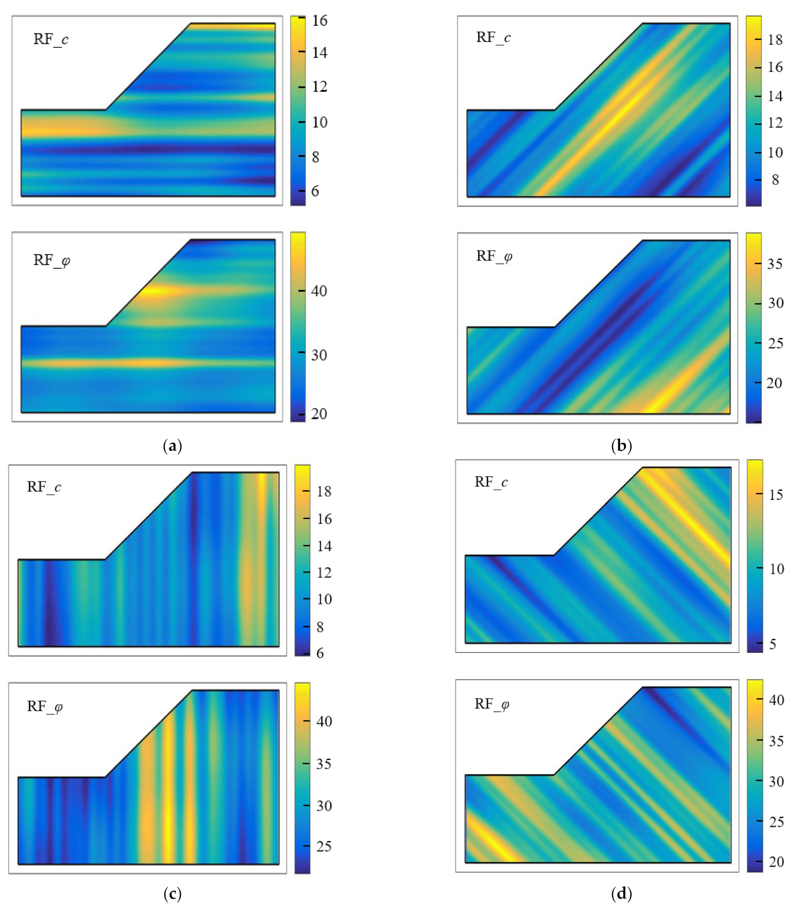
The realizations of cohesion and friction angle while considering the rotation of deposition orientations as 0°, 45°, 90°, and 135° were presented firstly, as shown in Figure 6. It should be noted that the rotation was counterclockwise. The horizontal and vertical autocorrelation lengths were respectively considered as 40 m and 3 m. The cohesion and friction angles were negatively correlated, and the cross-correlation coefficient was set to be −0.5. It can be observed from Figure 6 that a low value of cohesion was associated with a high value of φ and vice versa.

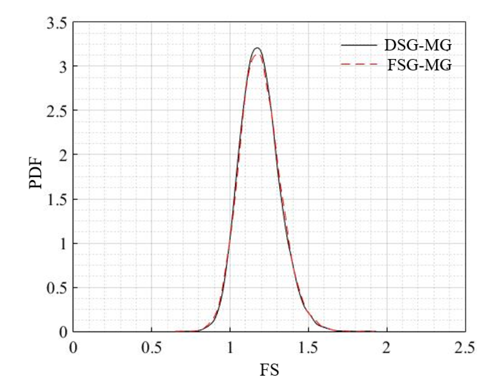
The probabilistic analysis with β = 45° was detailed. Two methods, DSG–MG and FSG–MG, were analyzed herein. The main results are summarized in Figure 7 and Figure 8. Ten thousand samples were set for the MCS calculation after the construction of the metamodel, and P_f was found to be 0.053 and 0.056 for DSG–MG and FSG–MG with COV_Pf being 4.2% and 4.1%, respectively.

Figure 7 depicts the PDF for the safety factor estimates using two methods. The curves were almost overlapping with each other. Moreover, the safety factor was almost distributed asymmetrically, and the FS values were mainly in the range of (0.5, 2).

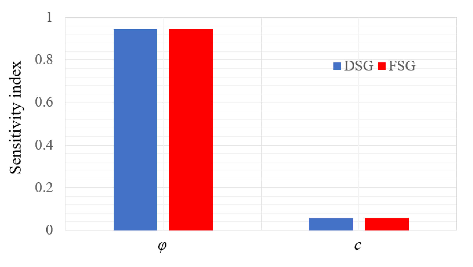
Figure 8 presents the Sobol indices of the two input variables. It is seen that the Sobol index of friction angle was far larger than the cohesion one, which means that the friction angle could have more significant influences on the model response compared to the cohesion. This can be clarified by the fact that the generation of a slip surface is strongly related to the friction angle for the limit analysis. Moreover, the friction angle is also involved in the work rates calculation. This finding is consistent with the works of Zhang et al. [29], in which they also reported a dominant effect of φ for the FS variation.

5. Validation and Efficiency Investigation of the Proposed Procedure

The introduction of the proposed procedure aimed to reduce the computational burden within the guarantee of the desired accuracy. A comparison with the existing study is firstly presented. The efficiency and accuracy of the analytical and probabilistic methods application on the slope with rotated random field consideration are then respectively detailed.

5.1. Comparison with a Previous Study

In order to validate the presented methods, a comparison with Cho [23] in the deterministic and probabilistic frameworks was performed. The results are summarized in

Table 2. Comparisons of the deterministic and probabilistic analyses results.

	Deterministic Results	Probabilistic Results
	FS	Pf	Number of Evaluations
Cho [21]	1.204	0.0138	50000
DSG–MG	1.201	0.0136	4200
FSG–MG	1.202	0.0130	4200

. The deterministic results were calculated by the mean values of soil parameters. For probabilistic analyses, the statistical properties of friction angle and cohesion were considered as random fields, as shown in Table 1. The autocorrelation lengths in the horizontal and vertical directions were, respectively, 20 m and 2 m. The cross-correlation coefficient was set equal to −0.5. The rotation of the random field was not considered in the comparison in order to be consistent with Cho [23].

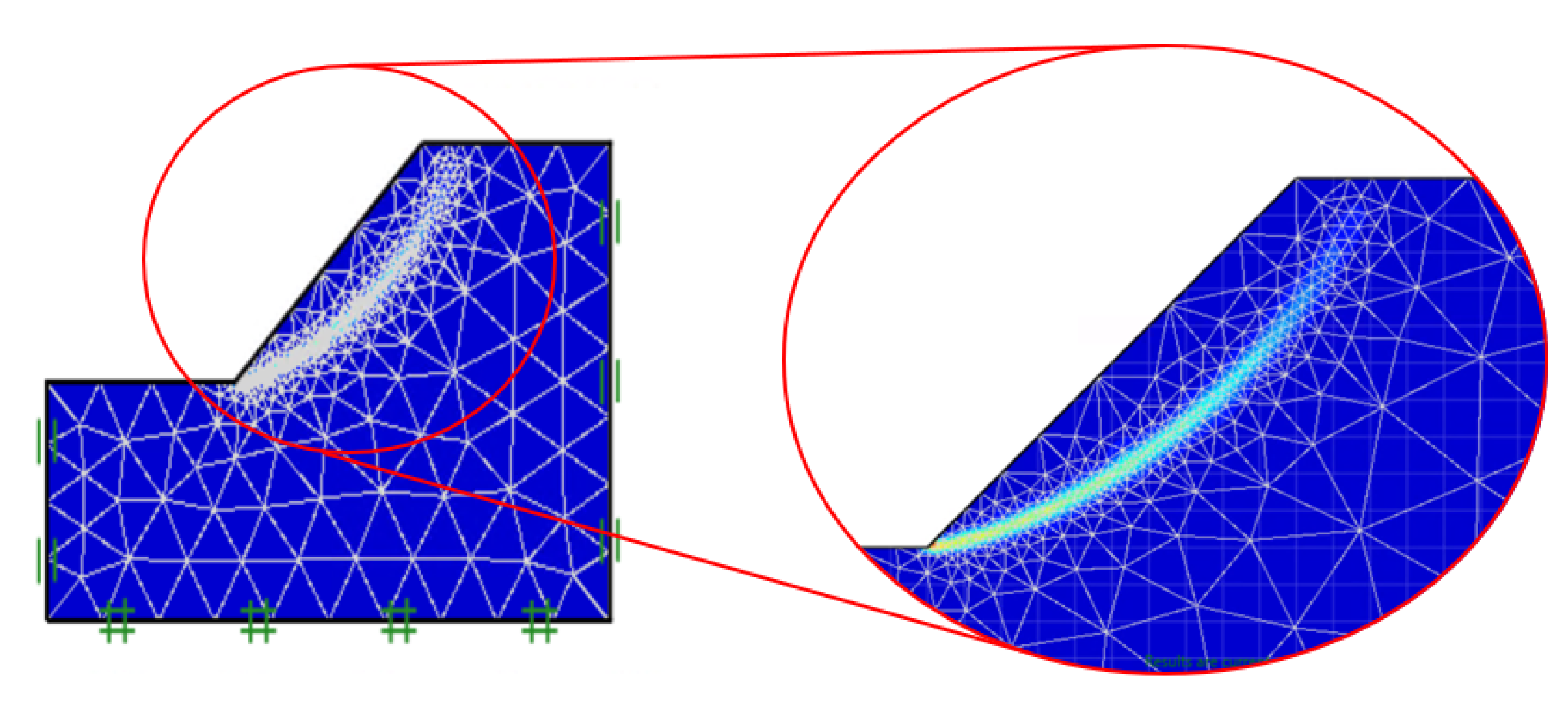
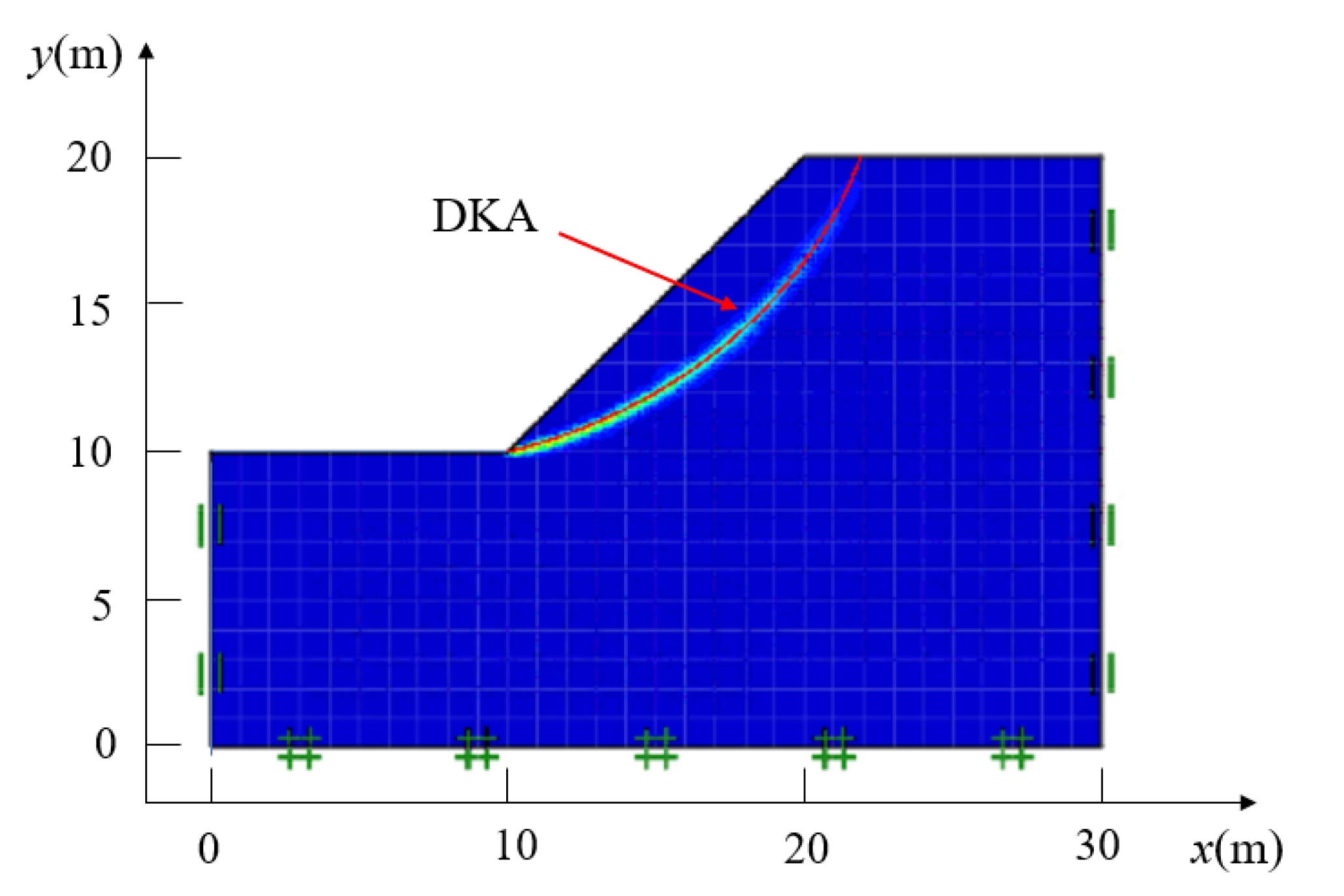
Good agreement in terms of safety factor and failure probability between this study and Cho [23] was observed. In addition, the discretization kinematic approach generated a similar failure surface with the numerical model, as presented in Figure 5. The comparison could validate the effectiveness of the proposed methods in the deterministic and probabilistic frameworks. Moreover, this study needed around 4200 simulations to meet the requirements of the accuracy, which is far less than the 50,000 calculations considered in Cho [23]. The efficiency of the presented methods is further discussed in detail in Section 5.

5.2. DKA Accuracy Considering Spatially Varying Soils and Rotated Anisotropy

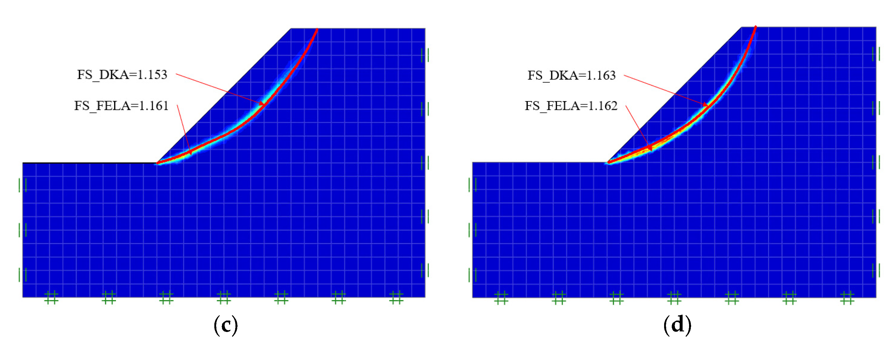
DKA is a versatile analytical method, since the failure surface based on this method is generated according to the spatially varied properties within the random field generation. Figure 9 depicts a comparison of FS and corresponding failure surfaces between two deterministic methods (DKA and FELA) for four random fields with different rotation angles of soil anisotropy (0°, 45°, 90°, 135°). It is seen that the FS values obtained by the two methods were always similar, with the error being no more than 1.2%. Concerning the critical failure surface, the analytical method DKA has the capacity to give consistent results with the FELA.

Moreover, as shown in Figure 7, the PDF curves obtained by the analytical model almost overlapped with those of the numerical model, which allows again the analytical method effectiveness to be validated and shows its accuracy in the probabilistic analyses.

It should be noted that the introduced deterministic approach DKA can alleviate the computation burden compared to the numerical method. This is very significant for the probabilistic analyses, which need numerous deterministic realizations. The FELA took around 60 s to perform one deterministic realization, whereas the computation time could be reduced to 5 s for the DKA, which could demonstrate the high efficiency of the analytical model DKA, which is used for the following discussions.

5.3. Comparison of SPCE/GSA and Direct MCS

A direct MCS analysis was performed to validate the probabilistic analysis results based on the metamodel SPCE/GSA. The comparison is summarized in

Table 3. Probabilistic results obtained by DSG–MG and MCS.

	Pf	Mean	Std	Number of Evaluations
MCS	0.056	1.192	0.130	10,000
DSG–MG	0.053	1.190	0.124	4000

and Figure 10. It was found that DSG–MG gave similar probabilistic results compared to the MCS. The PDF curve, as shown in Figure 10, was also close to the MCS, which indicates that the meta-model can provide rational information compared with the original computational model in the probabilistic analyses. However, it was seen that 4000 calls to the deterministic model were required for the DSG–MG, which is smaller compared to the direct MCS with 10,000 model evaluations.

Moreover, the introduction of GSA can significantly reduce the number of random variables. Taking l_h = 40 m and l_v = 3 m as an example, at least 168 variables are necessary for a variance error less than 10%, which means that 168 standard normal variables are considered to be input variables for the probabilistic analyses. Two random fields (friction angle and cohesion) were considered herein so that the dimension of the input space was 336. This is a high-dimensional stochastic problem, and it is cumbersome to carry out the probabilistic analyses. The metamodel SPCE/GSA can reduce the dimension of the input space from 336 to 41, which can improve significantly the calculation efficiency.

The above analyses demonstrate that the analytical method can capture accurately the spatially varied parameters within the random field and decrease the time of deterministic realizations. The SPCE/GSA can reduce the input variables dimension and permit one to construct a fast-to-evaluate metamodel based on the deterministic input–out sets. Therefore, the proposed DSG–MG procedure is efficient and can provide accurate estimations for the probabilistic analysis, which is used for the following parametric analyses.

6. Effects of Rotated Anisotropy Considering Different Influential Factors

Three parametric studies based on the proposed procedure DSG–MG are discussed, which include (1) the importance of rotated anisotropy consideration; (2) autocorrelation length influence; (3) the effects of cross-correlation between cohesion and the friction angle; and (4) coefficient of variation effects.

6.1. Effect of the Rotation Angle

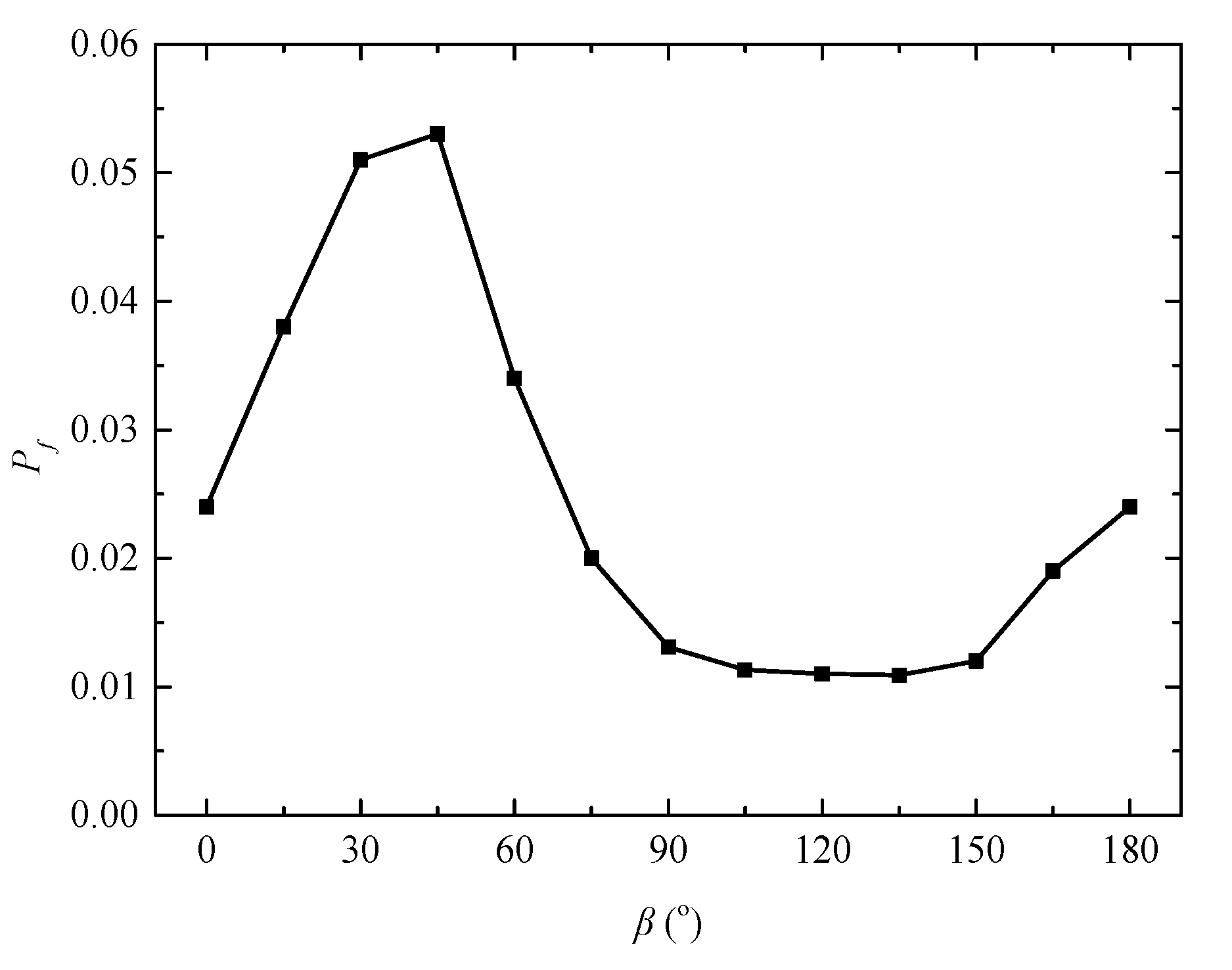
The rotation angle of anisotropy varied in the range 0° ≤ β ≤ 180°. Figure 11 shows the results of the failure probability under different values of β with an interval of 15°. It could be observed that the failure probability varied significantly with the anisotropy rotation angles. The value of P_f increased considerably, and when the β approached the slope inclinations (β = 45°), the failure probability reached the peak. After that, the P_f value decreased drastically until the rotation angle was approximately equal to 90°. This was followed by a slight fluctuation, and it reached its lower value when the anisotropic fabric was approximately perpendicular to the slope (β = 135°). The value of P_f increased until the random field was horizontal (β = 180°).

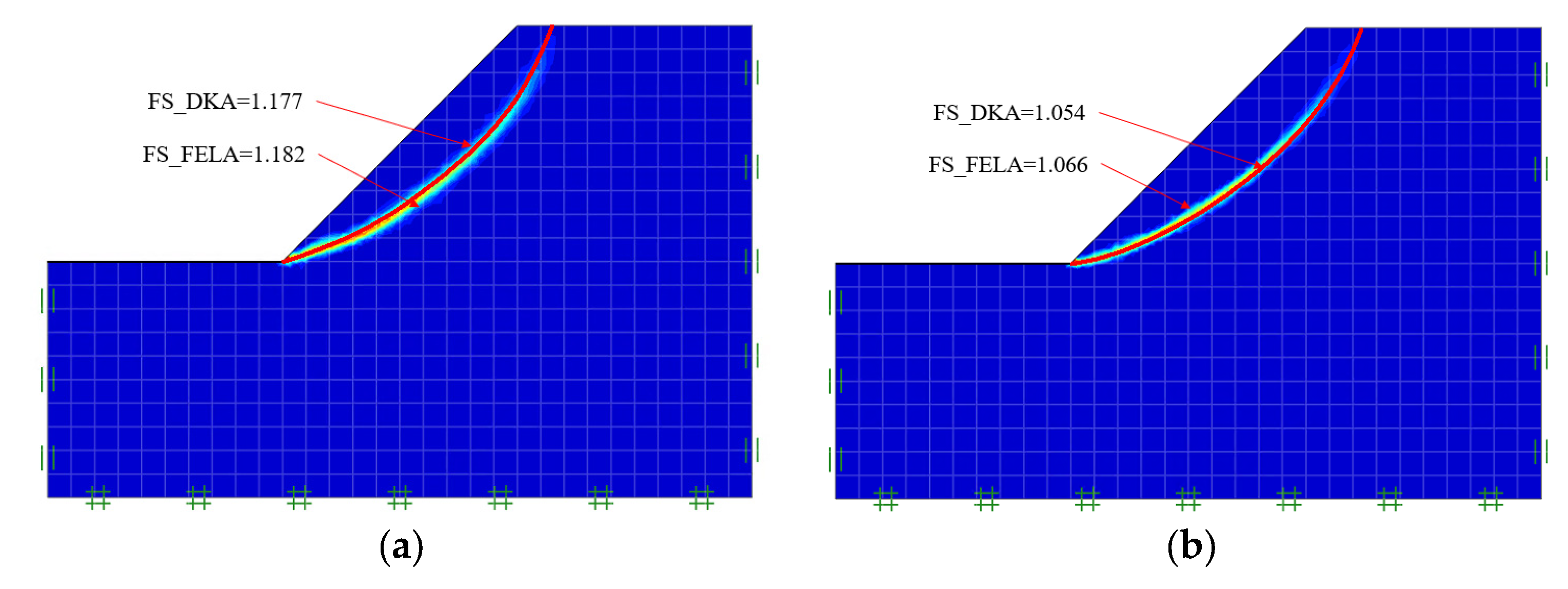
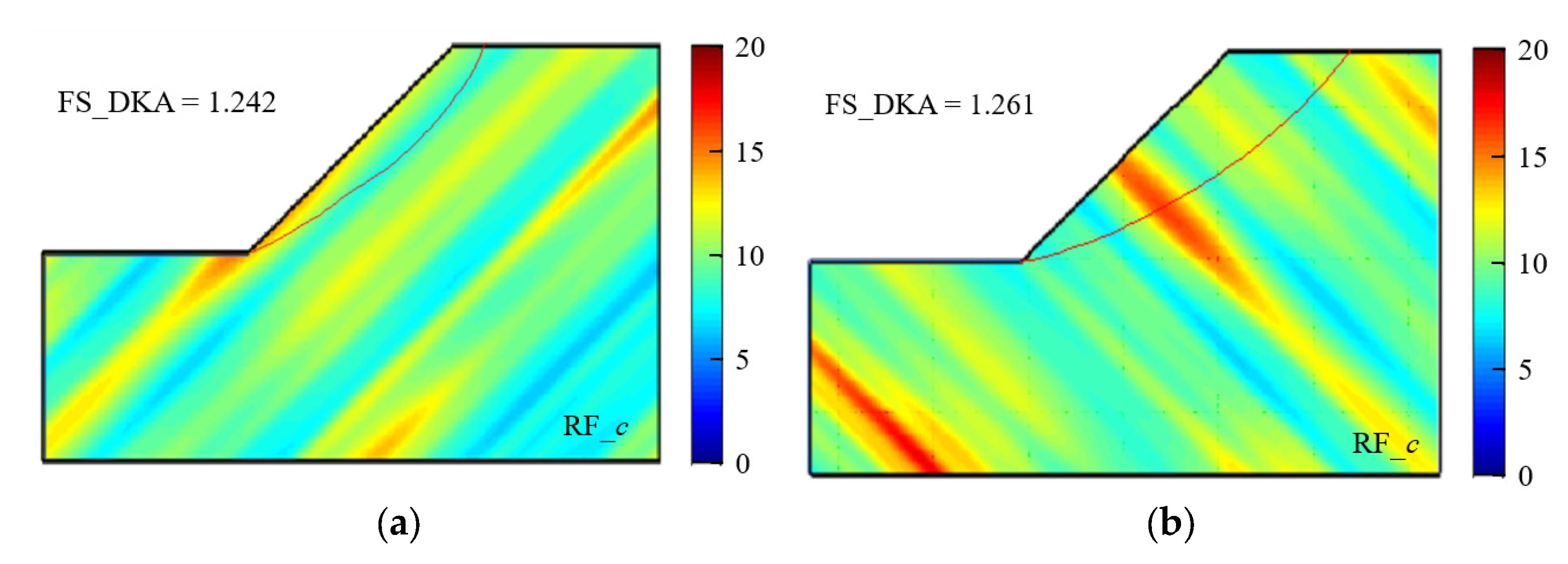
This finding is similar to previous works [6,7], which indicated that when the fabric orientation is parallel to the slope, a higher failure probability can be found. Conversely, a lower failure probability occurs when the fabric orientation is perpendicular to the slope. This is because the critical failure surface is dependent on the location of the weak soil patterns. When the anisotropy stratification is parallel to the surface, it is easier for the failure surface to pass through a single weak soil layer, as shown in Figure 12a, which leads to smaller safety factor and a high failure probability. 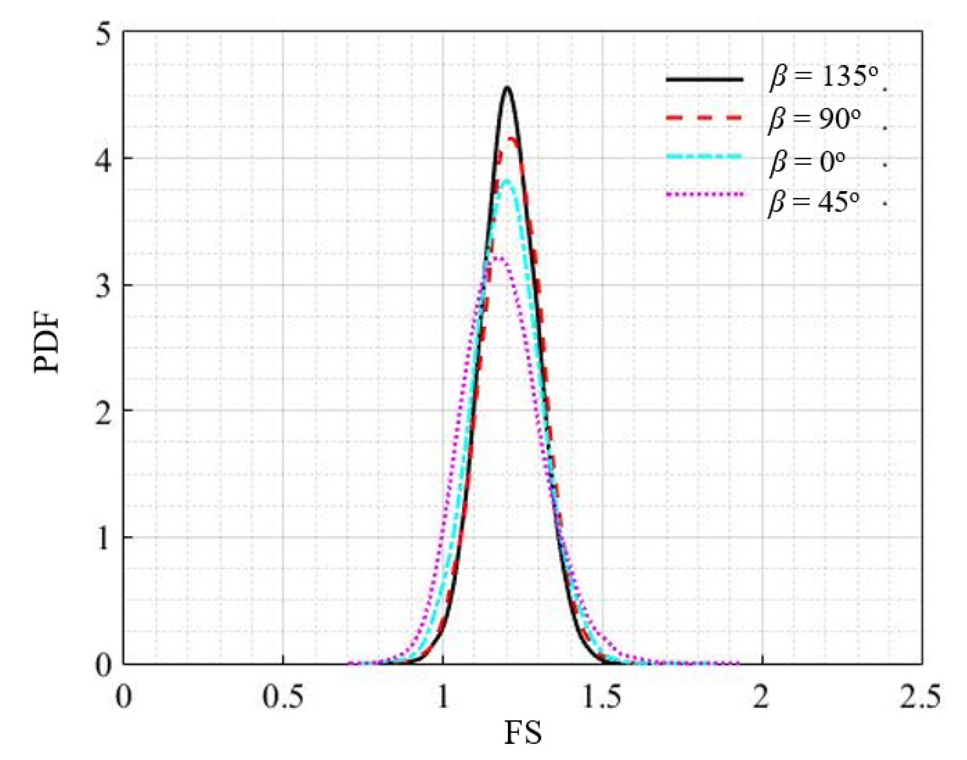Conversely, the failure surface is gentle, as presented in Figure 12b, when the soil stratification is perpendicular to the slope, and it leads to larger safety factors and a lower probability of failure. As seen in Figure 13, a tall and narrow PDF curve was observed when β = 135°, whereas a shorter and wider one was observed for the case of β = 45°, which means the variability of the acquired safety factor increased. Therefore, the rotational feature of the random field should be considered in practical engineering, particularly for cases where the stratification is approximately parallel to the slope inclination.

Table 4. Probabilistic results comparison with different values of random field rotation angle.

β (°)	Pf	Mean	Std	SC	Sφ
0	0.028	1.201	0.106	0.034	0.966
45	0.053	1.190	0.124	0.020	0.980
90	0.013	1.210	0.095	0.028	0.972
135	0.011	1.208	0.089	0.022	0.978

presents the probabilistic analysis results, which include the failure probability, statistical moments of FS, and Sobol indices of shear strength parameters, with β being 0°, 45°, 90°, 135°. It is noted that the mean safety factors were similar, while the standard deviation reached the highest for the case with β being 45°. Moreover, the rotation angle of anisotropy stratification had a slight influence on the Sobol indices. The Sobol index of the friction angle (around 0.98) was larger compared to the cohesion angle (around 0.02), which indicates that the friction angle affected sensitively the FS variability more than the cohesion for all the anisotropy stratification conditions.

6.2. Effect of the Autocorrelation Length

Figure 14 plots the variations of the failure probability under different autocorrelation lengths and rotation angles of anisotropy stratification. The results were obtained for l_v values of 2 m and 3 m and an l_h value of 40 m.

It was found that the failure probability was decreased with a decrease in autocorrelation length. This is because a higher autocorrelation length indicates that the soil shear strength is more strongly correlated, which can result in a relatively low variation. Therefore, the global average of the strength parameter changes a lot for different realizations, which results in higher variability of the obtained safety factors. Conversely, a small autocorrelation length can lead to more non-homogeneous zones, and smaller system response variation. It can also be interpreted by Figure 15 that the PDF of l_v = 2 m was narrower than in the case of l_v = 3 m, which showed a smaller variability. With increasing l_v, the PDF curve approached the PDF obtained using the random variables (infinite autocorrelation length), which had the most significant variation, and the failure probability was up to 0.103.

Moreover, the rotation angle made a more significant influence as the autocorrelation length increased. For example, the failure probability differences were, respectively, 0.042 and 0.025 for the case with l_v being 3 m and 2 m. Moreover, the autocorrelation length affected the failure probability more considerably when the stratification rotation angle was approximately equal to the slope inclination. Therefore, the autocorrelation length determination should be examined carefully, particularly for the case with rotated soil stratification.

Table 5. Probabilistic results comparison with different values of autocorrelation length.

lv(m)	Pf	Mean	Std	Sc	Sφ
2	0.026	1.204	0.104	0.017	0.983
3	0.053	1.190	0.124	0.020	0.980
40	0.073	1.204	0.146	0.030	0.970
100	0.077	1.208	0.149	0.031	0.969
Random variables	0.103	1.204	0.171	0.037	0.963

presents the probabilistic analysis results with different autocorrelation lengths. The failure probability and standard deviation of safety factors increased with the increase of the autocorrelation length, which is consistent with the results presented in Figure 14 and Figure 15. Moreover, the autocorrelation length effect on the Sobol index was slight, and the value of S_φ was far larger than that of S_c, indicating again the important role of friction angle.

6.3. Effect of the Cross-Correlation

Figure 16 shows the failure probability versus the cross-correlation coefficients with four random field rotation angles (0°, 45°, 90°, 135°). It was found that the cross-correlation coefficients influenced significantly the slope failure probability. With increases in the cross-correlation coefficient, the failure probability increased. This was because compared to a positively correlated correlation, a negative correlation means that lower cohesion values correspond to higher friction angle values, which can make the shear strength less uncertain. Figure 17 depicts the PDFs for different cross-correlation coefficients (−0.7, 0, 0.5); a taller and narrower PDF curve is presented with the decrease of the cross-correlation coefficient. This means that the safety factor variability decreased, and then the failure probability decreased. This finding is consistent with the results of Figure 16.

Moreover, the cross-correlation effects were more significant when the rotation angle of anisotropy stratification was equal to the slope inclination (45°). For example, the failure probability varied from 0.023 to 0.162 when β = 45°, while for the case with β = 135°, the values varied from 0.001 to 0.091. Similarly, the rotation angle influenced the failure probability more significantly for the cases with larger values of cross-correlation coefficient.

Table 6. Probabilistic results comparison with different values of cross-correlation coefficient.

r	Pf	Mean	Std	SC	Sφ
−0.7	0.023	1.208	0.094	0.014	0.986
−0.5	0.053	1.190	0.124	0.020	0.980
−0.25	0.085	1.204	0.142	0.137	0.863
0	0.111	1.201	0.157	0.255	0.745
0.25	0.143	1.204	0.178	0.449	0.551
0.5	0.162	1.199	0.193	0.629	0.371

summarizes the probabilistic analysis results under different values of cross-correlation coefficient with β being 45°. It is noted that the mean safety factors were similar while the standard deviation was increasing with the increase of the cross-correlation coefficient, which is consistent with the results of Figure 16. Moreover, it is noted that the Sobol index of cohesion was increasing with the increase of the cross-correlation coefficient, while that of friction angle presented an opposite trend. The value of S_C was even greater than that of S_φ when the cross-correlation coefficient was equal to 0.5. Therefore, in the rotated random field cases, the cross-correlation coefficient makes a considerable effect on the failure probability and sensitivity indices, which should be determined with caution in practice. The quantification of the cross-correlation was considered in the existing research [33,34,35], which is not further discussed in this study.

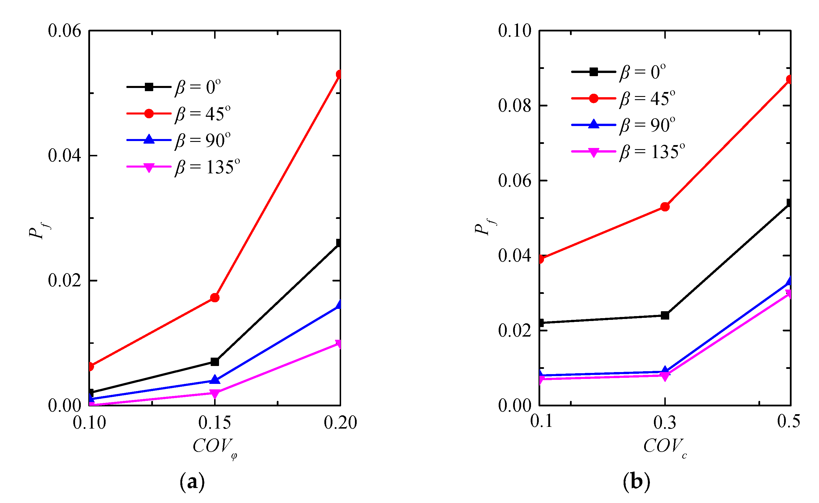
6.4. Effect of the Coefficient of Variation

Figure 18 depicts the effects of the two shear strength parameters (cohesion and friction angle) COV (COV_c and COV_φ) on the failure probability with four random field rotation angles (0°, 45°, 90°, 135°). The COV values of the friction angle and cohesion are respectively in the range of [0.1,0.2] and [0.1,0.5] [22].

It can be noted that COV had a significant influence on the failure probability, and the value of P_f increased with the increase of COV. This is because a larger value of COV led to more varied shear strength, which increased further the variability of safety factors. Taking the COV_φ as an example, it can be observed from Figure 19 that the PDF curve was wider with the increase of the COV_φ. Similar to the cross-correlation discussion, the rotation angle has a more important effect on the failure probability with the increase of the coefficient of variation.

Table 7. Probabilistic results comparison with different values of coefficient of variation.

COV	Pf	Mean	Std	SC	Sφ
COVc = 0.3
COVφ = 0.1	0.006	1.204	0.079	0.417	0.583
0.15	0.017	1.206	0.098	0.136	0.864
0.2	0.053	1.190	0.124	0.020	0.980
COVφ = 0.2
COVc = 0.1	0.039	1.216	0.120	0.011	0.989
0.3	0.053	1.190	0.124	0.020	0.980
0.5	0.087	1.196	0.134	0.225	0.775

provides the probabilistic analysis results with different values of coefficient of variation for the β = 45° case. It was found that the Sobol indices were strongly influenced by the COV values. Moreover, as presented in Figure 18 and Table 7, the value of COV_φ had more significant effects on the probabilistic results compared to the COV_c. For example, the Sobol index of friction angle increased from 0.583 to 0.980 with COV_φ varying from 0.1 to 0.2, whereas the difference was smaller with the variation of COV_c.

7. Conclusions

This paper presents a probabilistic analysis of slopes considering the rotated anisotropy within a random field framework. The proposed procedure DSG–MG, coupling the discretization kinematic approach (DKA), Sparse Polynomial Chaos Expansion (SPCE), Global Sensitivity Analysis (GSA), and Monte Carlo Simulation (MCS), is efficient and can provide accurate estimations for the probabilistic analysis. The analysis results are validated and some discussions are carried out. The conclusions drawn from this study are listed as follows:

(1)

The proposed procedure DSG–MG provides a good insight for the probabilistic stability analyses of slopes by the fact that the analytical method DKA can capture accurately the spatially varied parameters within the random field generation and can give rational results efficiently compared to the FELA ones (5 s and 60 s, respectively, for one deterministic calculation with the two methods); the metamodel constructed using SPCE/GSA can reduce the problem dimension and also the number of deterministic simulations by comparing with the direct MCS; several interesting results (the failure probability, probability density function, statistical moments of the model response, and sensitivity index of each variable) can also be obtained effectively.

(2)

The rotation of the anisotropic soil fabric pattern has a significant effect on slope stability. The failure probability is increased drastically when the rotation angle approaches the slope inclination. Using the traditional horizontal random field will then overestimate greatly the slope reliability, particularly for the cases with larger values of autocorrelation length, cross-correlation, and coefficient of variation. Conversely, the slope is safer when the rotated stratification is perpendicular to the slope inclination.

(3)

The failure probability is increased with the increase of autocorrelation lengths, coefficient of variation, and cross-correlation coefficient, and the effects of these parameters are more significant when the soil stratification rotation angle is close to the slope inclination, which should be determined with caution.

(4)

The rotation of soil stratification and autocorrelation length have almost no influence on the sensitivity index of the cohesion and friction angle, and the influence of the friction angle on the model response variance is higher than the cohesion angle. Conversely, the cross-correlation coefficient and coefficient of variation influence significantly the sensitivity indices, and the Sobol index of cohesion is increased with the cross-correlation coefficient r and coefficient of variation of cohesion COV_c increase. The friction angle case presents an opposite trend.

References

1. Ji, J.; Liao, H.J.; Low, B.K. Modeling 2-D spatial variation in slope reliability analysis using interpolated autocorrelations. Comput. Geotech. 2012, 40, 135–146. [Google Scholar] [CrossRef]
2. Jiang, S.H.; Li, D.Q.; Zhang, L.M.; Zhou, C.B. Slope reliability analysis considering spatially variable shear strength parameters using a non-intrusive stochastic finite element method. Eng. Geol. 2014, 168, 120–128. [Google Scholar] [CrossRef]
3. Li, X.Y.; Zhang, L.M.; Gao, L.; Zhu, H. Simplified slope reliability analysis considering spatial soil variability. Eng. Geol. 2017, 216, 90–97. [Google Scholar] [CrossRef]
4. Griffiths, D.V.; Huang, J. Probabilistic slope stability analysis using RFEM with non-stationary random fields. In Proceedings of the Geotechnical Safety and Risk V, Rotterdam, The Netherlands, 13–16 October 2015; pp. 1–7. [Google Scholar]
5. Ji, J.; Chan, C.L. Long embankment failure accounting for longitudinal spatial variation—A probabilistic study. Comput. Geotech. 2014, 61, 50–56. [Google Scholar] [CrossRef]
6. Zhu, H.; Zhang, L.M.; Xiao, T. Evaluating stability of anisotropically deposited soil slopes. Can. Geotech. J. 2019, 56, 753–760. [Google Scholar] [CrossRef]
7. Griffiths, D.V.; Fenton, G. Influence of anisotropy and rotation on probabilistic slope stability analysis by RFEM. In Proceedings of the 62nd Canadian Geotechnical Conference, Halifax, NS, Canada, 20–24 September 2009; pp. 542–546. [Google Scholar]
8. Huang, L.; Cheng, Y.M.; Leung, Y.F.; Li, L. Influence of rotated anisotropy on slope reliability evaluation using conditional random field. Comput. Geotech. 2019, 115, 103133. [Google Scholar] [CrossRef]
9. Leshchinsky, B.; Ambauen, S. Limit Equilibrium and Limit Analysis: Comparison of Benchmark Slope Stability Problems. J. Geotech. Geoenviron. Eng. 2015, 141, 04015043. [Google Scholar] [CrossRef]
10. Hou, C.; Zhang, T.; Sun, Z.; Dias, D.; Shang, M. Seismic Analysis of Nonhomogeneous Slopes with Cracks Using a Discretization Kinematic Approach. Int. J. Geomech. 2019, 19, 1–14. [Google Scholar] [CrossRef]
11. Mollon, G.; Dias, D.; Soubra, A. Two new limit analysis mechanisms for the computation of the collapse pressures of circular tunnels driven by a pressurized shield. In Proceedings of the 2nd International Conference on Computational Methods in Tunnelling, Bochum, Germany, 9–11 September 2009; pp. 849–856. [Google Scholar]
12. Du, D.; Zhuang, Y.; Sun, Q.; Yang, X.; Dias, D. Bearing capacity evaluation for shallow foundations on unsaturated soils using discretization technique. Comput. Geotech. 2021, 137, 104309. [Google Scholar] [CrossRef]
13. Budetta, P. Some remarks on the use of deterministic and probabilistic approaches in the evaluation of rock slope stability. Geosciences 2020, 10, 163. [Google Scholar] [CrossRef]
14. Ji, J.; Zhang, C.; Gao, Y.; Kodikara, J. Effect of 2D spatial variability on slope reliability: A simplified FORM analysis. Geosci. Front. 2018, 9, 1631–1638. [Google Scholar] [CrossRef]
15. Marelli, S.; Sudret, B. UQLab: A framework for Uncertainty Quantification in MATLAB. In Proceedings of the 2nd International Conference on Vulnerability, Risk Analysis and Management (ICVRAM2014), Liverpool, UK, 13–16 July 2014; pp. 2554–2563. [Google Scholar]
16. Zhou, S.; Guo, X.; Zhang, Q.; Dias, D.; Pan, Q. Influence of a weak layer on the tunnel face stability—Reliability and sensitivity analysis. Comput. Geotech. 2020, 122, 103507. [Google Scholar] [CrossRef]
17. Schöbi, R.; Sudret, B.; Marelli, S. Rare Event Estimation Using Polynomial-Chaos Kriging. ASCE-ASME J. Risk Uncertain. Eng. Syst. Part A Civ. Eng. 2017, 3, 1–12. [Google Scholar] [CrossRef] [Green Version]
18. Pan, Q.; Dias, D. Probabilistic evaluation of tunnel face stability in spatially random soils using sparse polynomial chaos expansion with global sensitivity analysis. Acta Geotech. 2017, 12, 1415–1429. [Google Scholar] [CrossRef]
19. Guo, X.; Dias, D.; Carvajal, C.; Peyras, L.; Breul, P. A comparative study of different reliability methods for high dimensional stochastic problems related to earth dam stability analyses. Eng. Struct. 2019, 188, 591–602. [Google Scholar] [CrossRef]
20. Kordjazi, A.; Pooya Nejad, F.; Jaksa, M.B. Prediction of ultimate axial load-carrying capacity of piles using a support vector machine based on CPT data. Comput. Geotech. 2014, 55, 91–102. [Google Scholar] [CrossRef]
21. Pan, Q.; Dias, D. An efficient reliability method combining adaptive Support Vector Machine and Monte Carlo Simulation. Struct. Saf. 2017, 67, 85–95. [Google Scholar] [CrossRef]
22. Guo, X.; Dias, D.; Pan, Q. Probabilistic stability analysis of an embankment dam considering soil spatial variability. Comput. Geotech. 2019, 113, 103093. [Google Scholar] [CrossRef]
23. Cho, S.E. Probabilistic assessment of slope stability that considers the spatial variability of soil properties. J. Geotech. Geoenviron. Eng. 2010, 136, 975–984. [Google Scholar] [CrossRef]
24. Liao, W.; Ji, J. Time-dependent reliability analysis of rainfall-induced shallow landslides considering spatial variability of soil permeability. Comput. Geotech. 2021, 129, 103903. [Google Scholar] [CrossRef]
25. Krabbenhoft, K.; Lyamin, A.; Krabbenhoft, J. OptumG2: Theory; Optum Computational Engineering: København, Denmark, 2016. [Google Scholar]
26. Sun, Z.; Li, J.; Pan, Q.; Dias, D.; Li, S.; Hou, C. Discrete kinematic mechanism for nonhomogeneous slopes and its application. Int. J. Geomech. 2018, 18, 04018171. [Google Scholar] [CrossRef]
27. Zhang, T.; Baroth, J.; Dias, D. Probabilistic basal heave stability analyses of supported circular shafts in non-homogeneous clayey soils. Comput. Geotech. 2021, 140, 104457. [Google Scholar] [CrossRef]
28. Pan, Q.; Qu, X.; Liu, L.; Dias, D. A sequential sparse polynomial chaos expansion using Bayesian regression for geotechnical reliability estimations. Int. J. Numer. Anal. Methods Geomech. 2020, 44, 874–889. [Google Scholar] [CrossRef]
29. Zhang, T.; Guo, X.; Dias, D.; Sun, Z. Dynamic probabilistic analysis of non-homogeneous slopes based on a simplified deterministic model. Soil Dyn. Earthq. Eng. 2021, 142, 106563. [Google Scholar] [CrossRef]
30. Sudret, B. Global sensitivity analysis using polynomial chaos expansions. Reliab. Eng. Syst. Saf. 2008, 93, 964–979. [Google Scholar] [CrossRef]
31. Guo, X.; Dias, D. A Practical Framework for Probabilistic Analysis of Embankment Dams. In Dam Engineering Recent Advances in Design and Analysis; IntechOpen: London, UK, 2021. [Google Scholar] [CrossRef]
32. Li, D.Q.; Zheng, D.; Cao, Z.J.; Tang, X.S.; Phoon, K.K. Response surface methods for slope reliability analysis: Review and comparison. Eng. Geol. 2016, 203, 3–14. [Google Scholar] [CrossRef]
33. Wang, Y.; Akeju, O.V. Quantifying the cross-correlation between effective cohesion and friction angle of soil from limited site-specific data. Soils Found. 2016, 56, 1055–1070. [Google Scholar] [CrossRef]
34. Wu, X.Z. Modelling dependence structures of soil shear strength data with bivariate copulas and applications to geotechnical reliability analysis. Soils Found. 2015, 55, 1243–1258. [Google Scholar] [CrossRef] [Green Version]
35. Di Matteo, L.; Valigi, D.; Ricco, R. Laboratory shear strength parameters of cohesive soils: Variability and potential effects on slope stability. Bull. Eng. Geol. Environ. 2013, 72, 101–106. [Google Scholar] [CrossRef]
Figure 1. Soil deposition with spatial anisotropy. (a) Horizontal anisotropy; (b) Rotated anisotropy.
Geosciences 11 00465 g001
Figure 2. Principle of the discretized failure mechanism of DKA.
Geosciences 11 00465 g002
Figure 3. FELA model with adaptive mesh refinement.
Geosciences 11 00465 g003
Figure 4. Flowchart of the analysis procedure D(F)SG–MG.
Geosciences 11 00465 g004
Figure 5. Geological profile of the reference case.
Geosciences 11 00465 g005
Figure 6. Realizations of random fields of cohesion and friction angle with r = −0.5; lh = 40 m, lv = 3 m. (a) β = 0°; (b) β = 45°; (c) β = 90°; (d) β = 135°.
Geosciences 11 00465 g006
Figure 7. PDFs of the obtained safety factor based on two methods.
Geosciences 11 00465 g007
Figure 8. Sensitivity analysis results.
Geosciences 11 00465 g008
Figure 9. Comparison of deterministic models with different values of random field rotation angle. (a) β = 0°; (b) β = 45°; (c) β = 90°; (d) β = 135°.
Geosciences 11 00465 g009aGeosciences 11 00465 g009b
Figure 10. PDFs of the FS obtained by DSG–MG and MCS.
Geosciences 11 00465 g010
Figure 11. Failure probability with different random field rotation angles.
Geosciences 11 00465 g011
Figure 12. Comparison of the slip surface with different random field rotation angles. (a) β = 45°; (b) β = 135°.
Geosciences 11 00465 g012
Figure 13. PDFs for different random field rotation angles.
Geosciences 11 00465 g013
Figure 14. Failure probability with different autocorrelation lengths and random field rotation angles.
Geosciences 11 00465 g014
Figure 15. PDFs for different autocorrelation lengths.
Geosciences 11 00465 g015
Figure 16. Failure probability with different cross-correlation coefficients and random field rotation angles.
Geosciences 11 00465 g016
Figure 17. PDFs for different cross-correlation coefficients.
Geosciences 11 00465 g017
Figure 18. Failure probability with different coefficients of variation and random field rotation angles. (a) coefficient of variation for friction angle; (b) coefficient of variation for cohesion.
Geosciences 11 00465 g018
Figure 19. PDFs for different coefficients of variation.
Geosciences 11 00465 g019