
Effective Continuum Approximations for Permeability in Brown-Coal and Other Large-Scale Fractured Media

Civil Engineering, Monash University, Clayton, VIC 3800, Australia
*
Author to whom correspondence should be addressed.
†
These authors contributed equally to this work.
Geosciences 2021, 11(12), 511; https://0-doi-org.brum.beds.ac.uk/10.3390/geosciences11120511
Submission received: 12 October 2021
/
Revised: 9 December 2021
/
Accepted: 10 December 2021
/
Published: 14 December 2021
(This article belongs to the Collection Early Career Scientists’ (ECS) Contributions to Geosciences)
Abstract
:The stability of open-pit brown-coal mines is affected by the manner in which water is transmitted or retained within their slopes. This in turn is a function of the in-situ fracture network at those mines. Fracture networks in real mines exhibit significant degrees of heterogeneity; encompassing a wide range of apertures, inter-fracture separations, and orientations. While each of these factors plays a role in determining fluid movement, over the scale of a mine it is often impractical to precisely measure, let alone simulate, the behaviour of each fracture. Accordingly, effective continuum models capable of representing the bulk effects of the fracture network are needed to understand the movement of fluid within these slopes. This article presents an analysis of the fracture distribution within the slopes of a brown coal mine and outlines a model to capture the effects on the bulk permeability. A stress-dependent effective-fracture-permeability model is introduced that captures the effects of the fracture apertures, spacing, and orientation. We discuss how this model captures the fracture heterogeneity and the effects of changing stress conditions on fluid flow. The fracture network data and the results from the effective permeability model demonstrate that in many cases slope permeability is dominated by highly permeable but low-probability fractures. These results highlight the need for models capable of capturing the effects of heterogeneity and uncertainty on the slope behaviour.
1. Introduction
The stability of an open-cut mine is strongly influenced by water flow within the in-situ fracture network. This is particularly true of brown coal mines: while solid coal is relatively impermeable e.g., [1,2], it contains numerous fractures that permit water to flow into the mine slopes. Excessive water retention within a slope may decrease the effective strength of the rock and lead to slope failure [3]. The effects of water can be represented as an overall reduction of shear strength in the rock [4,5,6]. However, this fails to account for the effects of fractures and its heterogeneity in the slope.
Numerical models are needed to predict the effect of fractures on the fluid retention in mine slopes. Discrete fracture models, which involve the explicit simulation of individual fractures, are often used to represent flow in fractured media [7,8,9,10,11]. These discrete fracture models often require extensive knowledge and data of the fracture network to explicitly simulate the fracture [12,13,14]. However, they are too numerically intensive to accurately represent large-scale simulations over long time frames, as required for mine slope stability [15,16,17]. A less numerically intensive approach is offered by effective continuum models. Effective-continuum-fracture models represent fracture permeability using estimates from the bulk material [18,19,20]. Such effective-continuum-fracture models are faster compared to discrete-fracture-permeability models that track the flow within each individual fracture.
Several of these continuum fracture models assume representative fracture properties for the entire fracture domain [16,21,22,23,24]. However, the heterogeneity of fracture networks strongly influences fluid flow trajectories [25,26,27] and may result in conditions that lead to slope failure, e.g., [28,29,30], or may dramatically affect transport properties within those networks, e.g., [31,32,33]. Nevertheless, attempts to capture heterogeneity with effective continuum models often still use average values for the model [34,35,36]. An average value for fractures may be accurate when there is a high fracture density and a narrow aperture distribution but may not properly account for the effects of material heterogeneity [37]. Hence, care must be taken when representing fractured media using continuous fields.
In this article, we discuss how best to represent the effect of the fracture network on the slope permeability using effective continuum models. We introduce probability-density-distribution functions that capture the variations in the fracture orientation, aperture, and spacing. These distributions are fitted to data obtained from a working brown-coal mine, AGL Loy Yang, in Victoria, Australia. Each distribution is evaluated by comparing their predictions of the fracture permeability with those from the original data.
We compare the results from the model with other representations of the fracture network and discuss the implications for slope permeability and transport properties and how it differs from models based on averaged values alone. By incorporating the fracture distribution in the numerical model, we are able to capture the effects of fracture heterogeneity. This model can then be applied in other contexts such as slope stability to highlight areas of high fluid retention that may cause slope failure e.g., [30]. The method used here to capture fracture heterogeneity in open-cut mines can also be applied in other fields such as underground tunnelling and shale gas where heterogeneous fractures often dictate the fluid or gas flow [38,39,40,41].
2. Model Description
In this section, we outline the theoretical basis for the fracture network model. We first introduce the basic effective continuum model representing the joint-set permeability and describe how that model can be expanded to account for variations in the joint properties. Next, we introduce different methods to capture the distributions in both the joint orientation and the aperture and spacing of the fractures. These models are then tested against data obtained from the fracture network distribution in a brown coal slope from the AGL Loy Yang mine in the following section.
2.1. Effective Fracture-Set Permeability
The effective continuum model introduced here assumes that the permeability of a mine slope can be determined from the expected transmissibility of its in situ fracture network [42]. Each individual fracture’s permeability is estimated based on a parallel plate approximation:
where is the permeability of the fracture and h is the hydraulic aperture [43,44,45,46,47]. As perfectly smooth fractures do not exist in nature, the permeability is affected by the fracture roughness and other geometric properties. Due to this, the hydraulic aperture is not equal to the mechanical aperture of the fracture, and this estimate should be viewed as an upper bound of the fracture permeability [48]. Nevertheless, the mechanical aperture and the hydraulic aperture are approximately equivalent for fractures with large apertures [49,50]. Assuming there exists a set of fractures separated by a spacing d, the three-dimensional permeability becomes:
where is the Kronecker delta and is the fracture normal calculated from the dip and strike [51,52].
The hydraulic aperture, h, is sensitive to changes in the in situ stress conditions. Several models have been proposed to capture this relationship, for example: Seidle et al. [53], Liu & Rutqvist [54], Chen et al. [55] and Yan et al. [56] employ the following equation:
where is the fracture compressibility, is the initial hydraulic aperture, and is the effective stress. The effective stress is defined as the stress acting perpendicular to the fracture less the pore pressure. The fracture compressibility measures the change in aperture as a function of the change in applied stress:
where is the fracture porosity [55,57,58]. Fracture compressibility is difficult to measure; however, an extensive review by Tan [59] reports a range of values up to 0.2 MPa for brown coal.
Multiple joint sets are represented in the effective continuum model as a superposition of their individual contributions:
where N is the number of joint sets and is the permeability of the nth joint set. Note, however, that the effective stress on each joint set will differ due to differences in the orientations of the fractures.
No real-world fracture network matches the idealized description outlined above. Fractures are not uniformly spaced, their orientations and apertures vary, and their measurement is prone to error and uncertainties. The variability in fracture properties makes it difficult to represent the heterogeneity in the fracture network explicitly. Thus, there is a need to adopt effective averaging procedures that capture the essential physics of the fracture system.
Under the simplest approach—one typically adopted in effective continuum models—it is assumed that the fracture network can be represented by a given number of principal joint sets. The number and orientation of joint-sets is determined using the median dip, the dip direction, and the fracture separation. However, within those joint sets there are additional variations in fracture aperture, spacing, and orientation. In the following sections, we introduce different functions and methods that we use to describe these distributions. Later, in Section 3, we consider how well these methods capture the characteristics of the fracture network from the AGL-Loy Yang mine.
2.2. Representing Joint Aperture and Separation
The distribution of fracture apertures and spacings is often described using log-normal probability distributions. Here, we also consider a second distribution function, the log-beta distribution. In Section 3, we compare the ability of both functions to describe an actual fracture data set.
The log-normal distribution is fitted by calculating the cumulative probability for each spacing or aperture and minimising the combined difference with the cumulative probability from the original data set. For a log-normal distribution, the Cumulative Distribution Function (CDF) is:
where is the log-normal cumulative distribution function of x, is the error function, is the log-mean, and is the log-standard deviation.
Here the log-normal distributions are fitted to both the fracture aperture and the inter-fracture separation (i.e., the distance between each fracture less the fracture aperture). Fitting to the inter-fracture separation, rather than the fracture separation, ensures that the fracture aperture is never greater than the separation between fractures.
The log-normal distribution has a disadvantage, however, in that it is unbounded. There is always a small but finite probability of generating an unphysically large value. To overcome this deficit, the fracture properties were also fitted with log-beta distributions.
The log-beta function is similar to log-normal distributions in that it fits a probability distribution to the natural log of the underlying data. The standard beta distribution is restricted to , and thus an adjustment must be made for the range of values in the log-beta function.
The CDF of the log-beta function is:
where, and the limits of the integral are given by ; is the gamma function with and as the two shape parameters.
2.3. Representing the Distribution of Joint Orientation
Given a set of fracture data that include the joint orientation, the aperture, and the spacing, the stress-dependent permeability of the entire system can be estimated from the equations given in Section 2.1.
A probability-density distribution based on the phi-theta grid can be produced to represent the distribution and uncertainty of a single joint set. Here, a weighted Gaussian distribution is used to show how the fractures in the joints vary about their average orientation.
The probability-density-distribution function for a single joint set is assumed to be symmetric about a principal direction with an approximately Gaussian distribution, whose orientation is defined by a second vector that lies perpendicular to :
where describes a probability density function for finding a fracture with normal in a joint set described by a principal direction , and and are the standard deviations along and , respectively.
We find the values of , , , and that best match the observed distribution of fractures by comparing the discrete set of fractures with the probability-density distribution of the joint set. This is accomplished by introducing a weighting function that maps a specific fracture orientation to all other orientations. For the discrete fracture network, this is given as:
where the sum is over the discrete set of fractures. In this way, the discrete fracture set is converted to a continuous representation that we can compare to the probability-density-distribution function for the joint set once it has been similarly weighted:
where here the integral is taken over all possible fracture orientations.
The misfit between our target function and the weighted probability-density distribution function is given by
To fit the probability-density distribution to the fracture set, we searched for the values of , , , and that minimized this misfit. The integral is evaluated using a quadrature rule:
where are quadrature weights, and i and j refer to grid indices in the azimuthal () and the polar () axes, respectively.
3. Fracture Network Representation
The previous section introduced several methods to represent the distribution of properties in the fracture set. Here, we evaluate these methods by testing their ability to match the distribution of fracture data obtained in a real-world fracture network, from surveys taken at the AGL Loy Yang brown-coal mine. The separate distributions are assessed with regard to their ability to represent not only the distribution of fracture properties but also their ability to reproduce fracture networks with similar permeability distributions.
3.1. Fracture Network
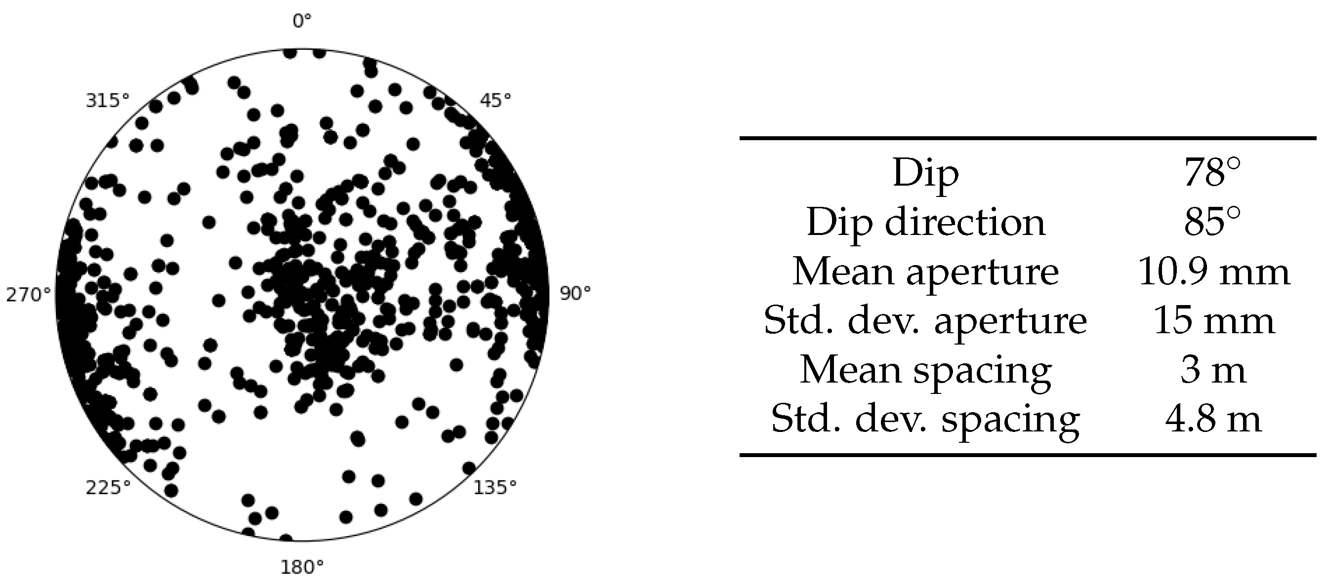
As an example, data from the fractures in the AGL Loy Yang coal mine are plotted on a stereonet given in Figure 1. The fractures have a median dip of 78 and a dip direction of 85. The fracture apertures have a mean value of 10.9 mm with a standard deviation of 15 mm, while the fracture spacing has a mean of 3 m with a standard deviation of 4.8 m (as noted in Figure 1).
We apply the equations in Section 2.2 and Section 2.3 to determine a probability distribution that accurately represents the fracture network. Firstly, the distributions of the fitted fracture apertures and spacings are described in Section 3.2. Following this, Gaussian distributions are applied to the fracture orientations as described in Section 3.3.
3.2. Fracture Spacing and Aperture
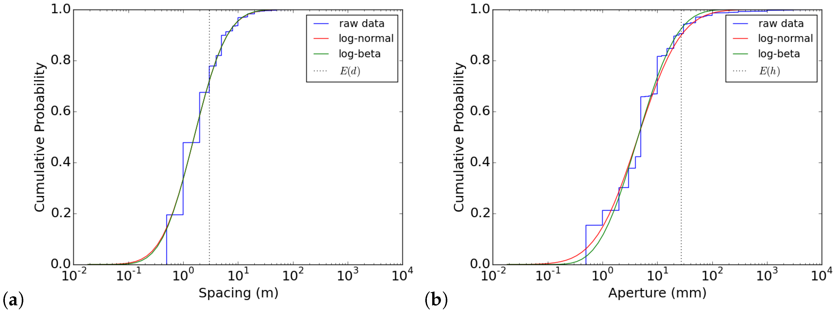
We apply the log-normal and log-beta distributions described in Section 2.2 to represent the fracture spacing and apertures in the raw data. The cumulative-distribution functions of the raw data and the fitted log-normal and log-beta functions of the fracture apertures and separations introduced in Equations (6) and (7) are shown in Figure 2. Both the standard log-normal distribution and the log-beta distributions demonstrate an excellent fit for the underlying raw data of apertures and separations, similar to reported distributions for other fracture sets [60,61].
For the purpose of this study, the range of the log-beta function was set to three log-standard deviations on either side of the log-mean of the data (i.e., ). This resulted in a distribution that captures the bulk of the data but eliminates the effect of the long-tail found in the log-normal distribution. The two shape parameters ( and ) for the log-beta distributions were found by minimizing the misfit between the raw cumulative distribution function from the data and that given by the fitted log-beta function.
The mean permeability of the fractures, , from the raw data ( m) was over two orders of magnitude greater than the permeability determined from the mean spacing and aperture (e.g., m). In comparison, the expected permeability from the log-normal fits was determined to be m, whereas the expected permeability of the log-beta distribution was m.
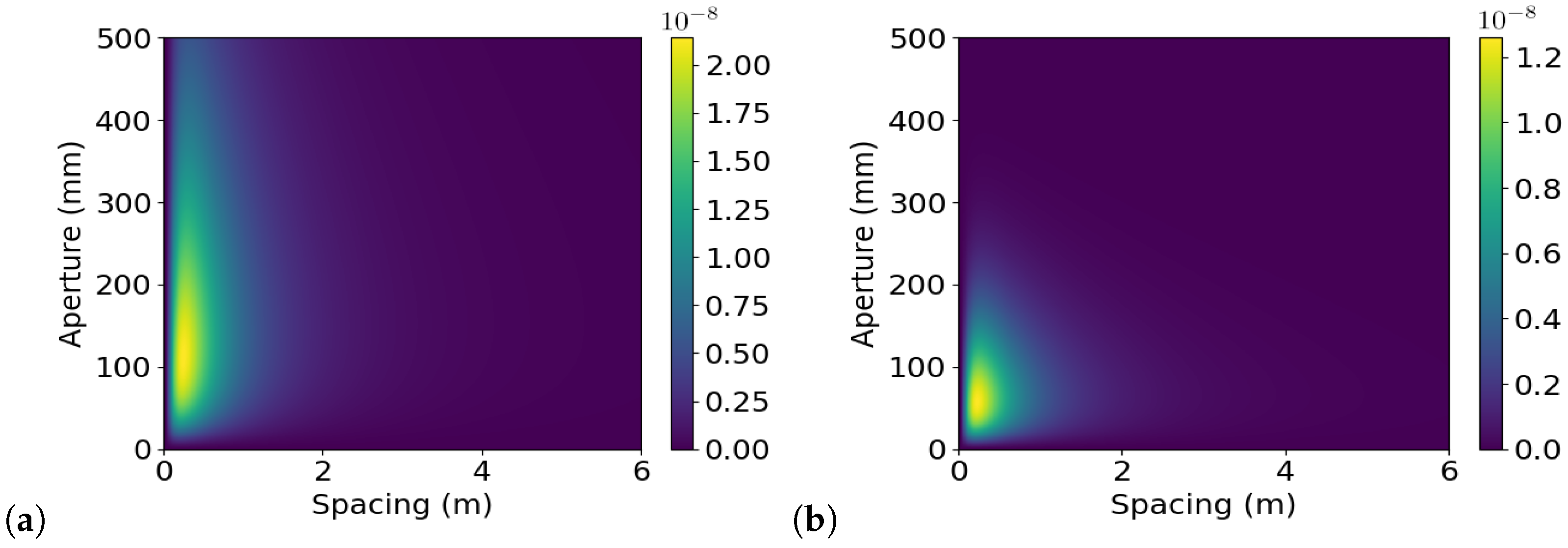
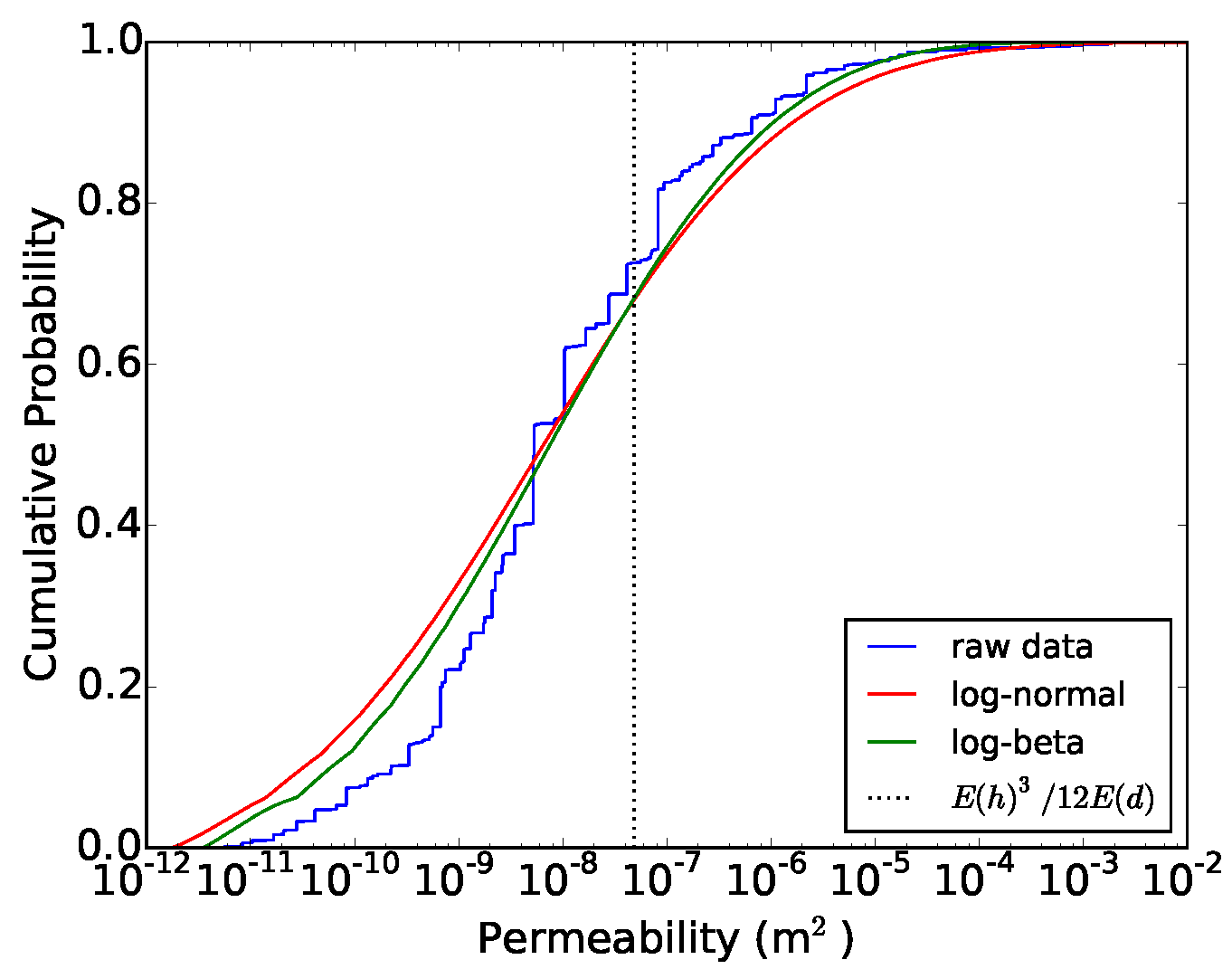
The major contribution to the permeability for both the log-normal and log-beta distributions arises from relatively large apertures (10–20 cm) with a small fracture separation (less than one meter) (Figure 3). Although fractures in this range are extremely rare, the cubic dependence on the aperture exaggerates their influence on the expected permeability. Compared to the raw data, the log-normal distribution over-estimates the permeability, whereas the beta distribution gives an under-estimate—as it limits the range and lowers the probability of large fractures. Nevertheless, both functions yield similar distributions to that given by the raw fracture data (Figure 4).
The small number of fractures with large permeabilities result in highly variable average permeabilities that are sensitive to the sample size. This results in difficulty when making a direct comparison between the mean permeabilities of the raw data and the fitted probability distributions.
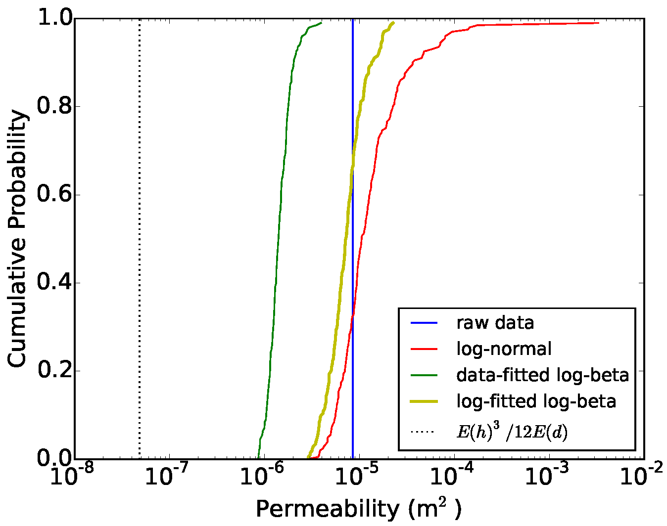
Figure 5 plots the distributions of average permeability obtained from random samples from the log-normal and log-beta distributions equal in size to the number of fractures in the raw data. The average permeability of the raw data (vertical blue line) and and the permeability obtained from the average fracture aperture and spacing (vertical dashed line) are also included for the purpose of comparison.
Comparing the mean fracture permeabilities of the raw data and random samples from the fitted probability distributions shows that the sub-sampled permeabilities of the fitted distributions are generally lower than their means. This is due to the tendency to not sample the high-permeability but low-probability fractures. For this reason, although the log-beta function arguably provides a better fit to the raw fracture distribution, it fails to match the raw permeability for any of the sample realisations (demonstrated by the green and blue lines in Figure 5).
Conversely, sub-samples from the log-normal distribution produce higher mean permeabilities. As a result, the raw data permeability is within the range of values produced by sampling from the log-normal distribution (demonstrated by the red and blue lines in Figure 5). On average, subsamples from the log-normal distribution predict a lower average permeability to that of the raw data that are sampled approximately 30% of the time. However, the unbounded nature of the log-permeability means that subsamples from the log-normal distribution often significantly over-estimate the observed permeability.
Fitting the beta function directly to the sample data fails to represent the probability of the larger aperture fractures and hence skews the permeability calculation. On the other hand, while the log-normal permeability produces a range that better captures the observed permeability, its unbounded nature results in unrealistically high permeabilities in many cases. However, these deficits may be overcome by fitting the beta function to the log-normal distribution of the apertures. This new log-beta fit has the advantage of being able to capture the effects of the high-permeability samples while removing the possibility of excessively large fractures that the log-normal distribution includes. This produces a sub-sampled distribution that includes the observed expected permeability but excludes extremely large fracture apertures (Figure 5 yellow line).
3.3. Fracture Orientation
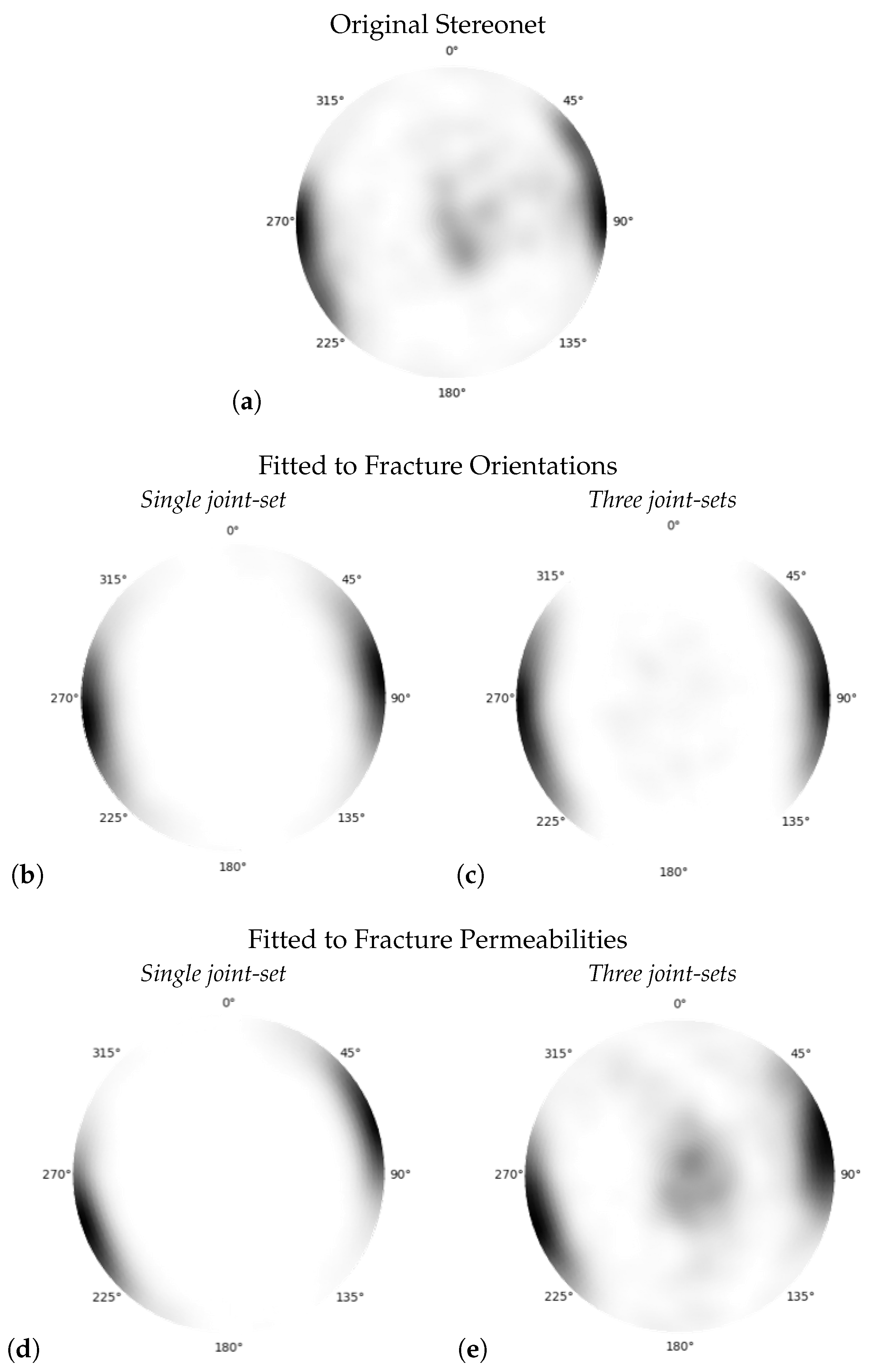
In this section, we consider how best to match the distribution of the fracture orientations. We apply the equations in Section 2.3 to determine a suitable fit to the data provided by AGL Loy Yang. Figure 6a is generated by applying the weighting function in Equation (9) to a sample of 1000 fracture observations from the original data.
Figure 6b,c are generated by fitting the distribution to the given in Equation (9) to discrete fracture density using the method outlined in Equations (11) and (12). Figure 6b applies a single Gaussian distribution and can only capture a single joint set. Thus, it overemphasises the dominant vertical fractures. Figure 6c applied three Gaussian distributions and captures some of the horizontal fractures in the stereonet. However, it still overemphasises the dominant vertical fractures and underperforms when capturing the horizontal joint set.
The fits to the probability distribution of the fracture sets provide an accurate representation of the overall joint orientations. However, because the fit tries to match the fracture density rather than the permeability, the effect of the main joint set are overemphasized, and the minor joint sets are not adequately captured.
In an effort to maintain an accurate representation but generate a fracture distribution that more faithfully reproduces the permeability, we also considered a second approach in which the joint set is instead fitted to the permeability distribution. Similar to fitting the probability-density distribution, we also searched for the values of , , , and to fit the permeability distribution to the permeability of the fracture data set. However, instead of minimising the cumulative difference between fracture densities, we compared the cumulative probability distribution of the raw and fitted permeabilities.
To isolate the effect of the fracture orientation as opposed to the other fracture properties, we considered how the permeability distributions of the original fracture set compare with the fitted distributions under the assumption of constant fracture apertures and spacing.
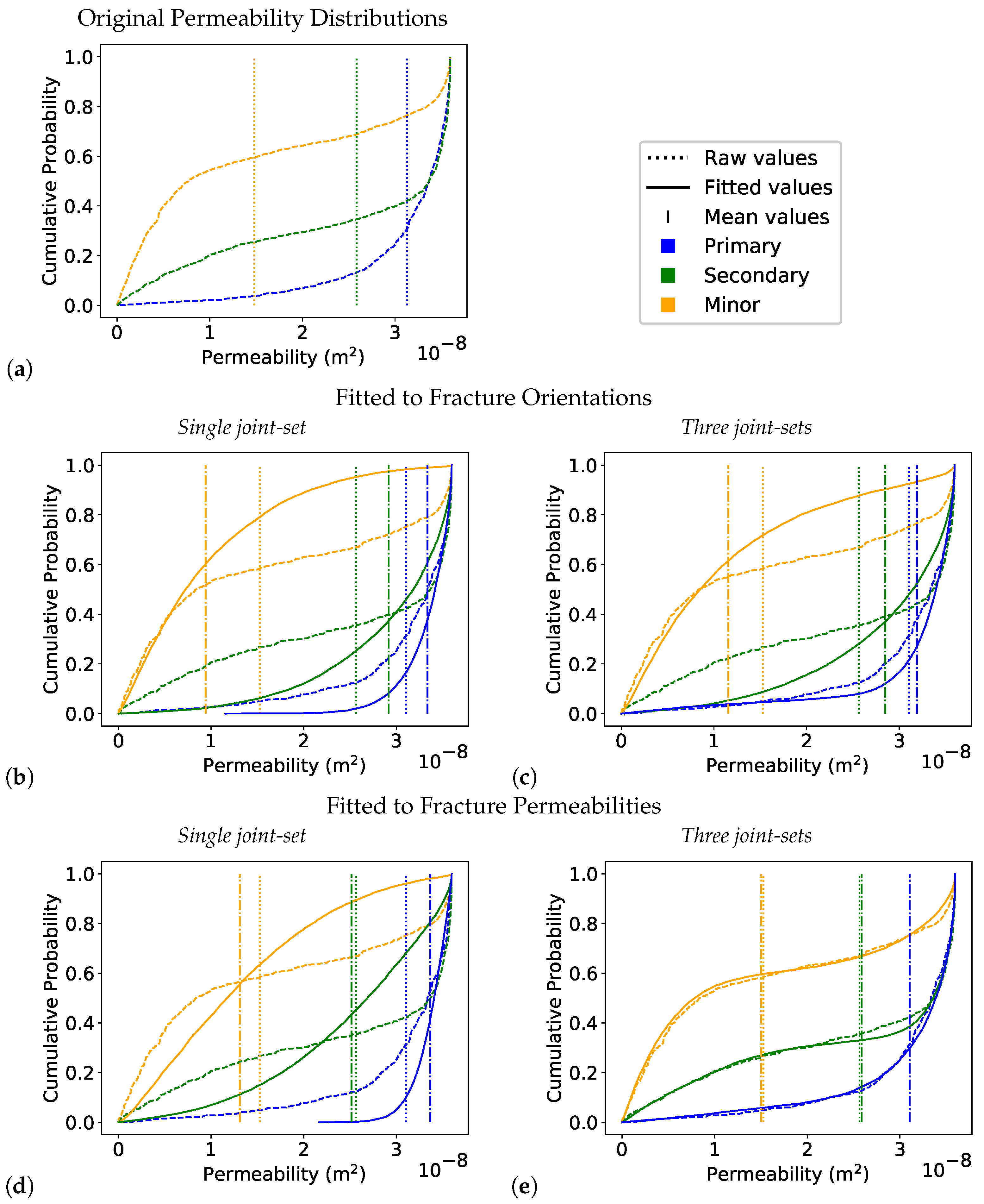
Cumulative distribution plots of the permeability for the original data and each of the fitted distributions are given in Figure 7. The permeabilities along three axes were considered (), corresponding to the principal axes of the expected permeability for the raw data. To create the cumulative permeability distributions in the plots, we randomly generated 10,000 fractures from the fitted orientation distributions and calculated their permeabilities along the principal directions from
where is the permeability of each individual fracture along the “nth” principal direction, . These values were then collected for each of the randomly generated fractures and sorted to produce the cumulative distribution plots in Figure 7.
Figure 7a shows the cumulative distributions of the permeabilities for the raw fracture data. Two of the the principal axes showed very similar permeabilities due to the preferential orientation of the fractures shown in Figure 6a. Nevertheless, the average permeability along the minor axis was more than half that of the major and secondary axes, due to the scatter in the fracture orientations.
The permeability distributions for the normal fits to the fracture orientations are shown in Figure 7b,c. The single normal fit to the fracture orientations (Figure 7b) is able to match the maximum and minimum permeability (e.g., the range) and has features that make it qualitatively similar to the raw distribution. However, the expected permeabilities fails to match those from the raw data. Because the single distribution only captures the dominant direction, the principal and secondary axes are too close to the maximum values. Likewise, the expected permeability along the minor axis is significantly less than the actual expected value. As a result, the model would grossly underestimate transverse flow within the fracture network. Increasing the number of distributions in Figure 7c improves the fit slightly, but the expected values remain underestimated for the minor axis and overestimated for the major and secondary axis.
To address the mismatch in the mean permeabilities observed in Figure 7b,c, we fit the fracture orientations by minimising the least-squared difference with the continuous permeability directly. As might be expected, fitting the distributions to the permeabilities themselves results in a significantly better fit, even for only one joint set (Figure 7d). The expected permeabilities along each of the principal axes (vertical lines) are much closer to those from the original data than even the three-joint set fit to the fracture distribution (Figure 7c). When three distributions are used to the match the permeability, the fit is excellent, especially for the expected permeabilities along each axis (Figure 7e). Moreover, even though the permeability is fitted rather than the fracture orientations, the fit nevertheless does a better job of capturing the the off-axis fracture orientations (Figure 6e).
4. Results and Discussion
To illustrate the effects of the different fracture-permeability distributions on the fluid flow, the numerical model was implemented within the Multiphysics Object-Oriented Simulation Environment (MOOSE) produced by the Idaho National Laboratory. MOOSE simulations have been used to couple multiple physics processes—in particular, coupling between solid mechanics, fluid flow, and heat conduction [62,63]. Here, we used a modified version of the Porous Flow module for our hydromechanical coupling [64]. Under this model, each cell in the finite-element simulation is assigned a permeability determined by sampling the fitted fracture-aperture distributions and orientations described in Section 3 and then calculating the effect on the permeability using the process outlined in Section 2.1. The sampled values are recorded and—in the case of the fracture apertures—updated in each timestep to capture changes to the permeability in response to changing effective stress conditions. By tracking the fractures in this manner, we are able to capture the effects of fracture heterogeneity and anisotropy on the fluid flow.
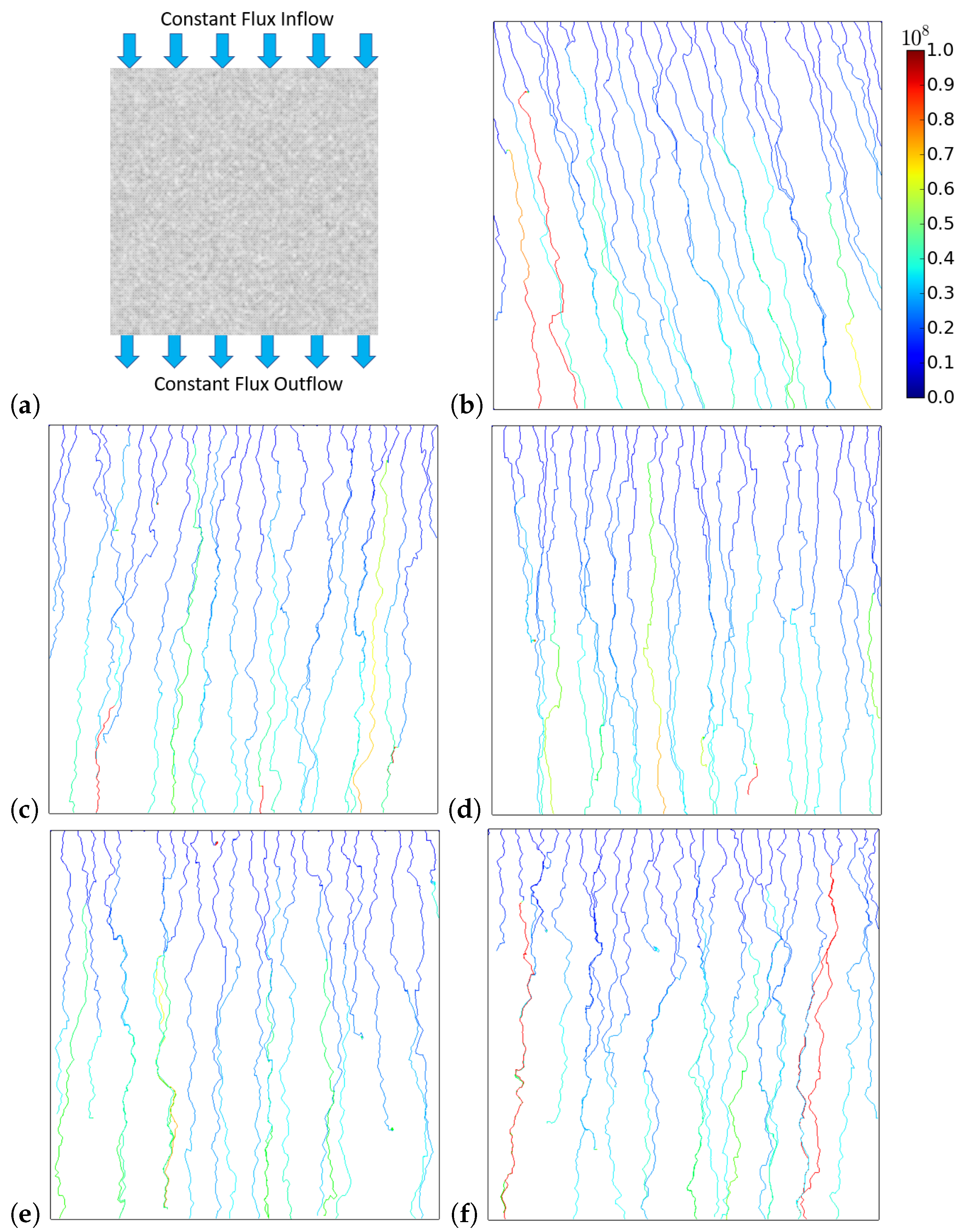
In Figure 8 and Figure 9, we show the effect of the different fracture orientations on the regional fluid flow. To illustrate the effect of the distributions on the flow profile, we compared simulations of the horizontal and vertical flows through a rectangular region. The plots compare the fluid flow streamlines and retention time of each of the fracture distribution models. The same variable aperture field was kept for each simulation. Constant flux-inflow and -outflow boundary conditions were applied on each boundary in the direction of flow, while periodic boundary conditions were applied in the transverse direction.
In the case of the vertical flow, which is roughly in line with the dominant fracture plane, all of the simulations produced flow paths with similar geometries. Comparing the streamlines of the different permeability distributions there was little effect on the direction of flow. However, with three Gaussian fits to the permeability (Figure 8f), there were more streamlines with a longer retention time, indicating lower vertical permeability. Each of the permeability distributions had significantly higher permeability in the vertical axis and showed little difference in the streamline geometries despite variations in retention time (Figure 10).
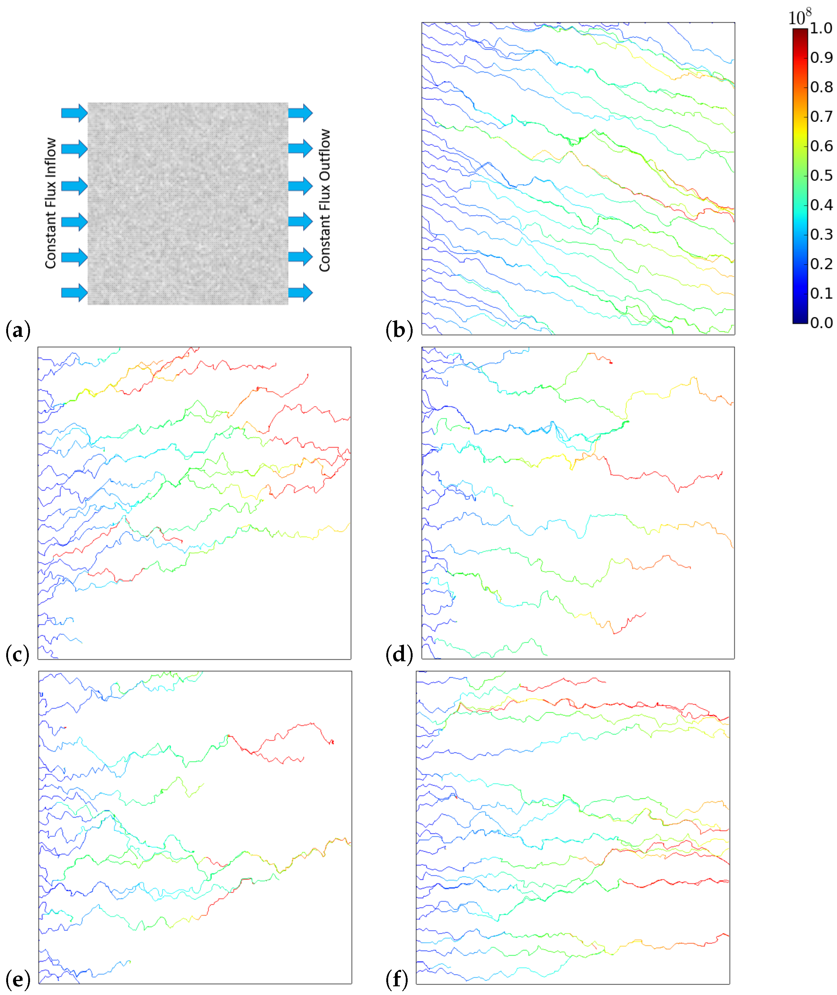
However, the differences in the streamline geometries are more pronounced when horizontal flows were considered (Figure 9). The constant fracture orientation results in a highly preferred flow direction as seen in Figure 9b. The streamlines in Figure 9d and e have limited horizontal flow as there are many areas of stagnation. This occurs as those models under-represent the horizontal connectivity of the fracture network. In contrast, Figure 9f uses the sampled data from three Gaussian distributions to the raw permeability. As a result, it contains areas of higher horizontal permeability that allow for more direct fluid flow. Using fracture orientation values taken from a single fit to the fracture density also produces more flow paths as seen in Figure 9c. However, these streamlines deviate upwards and have longer residence times due to the significantly higher vertical permeability and the low horizontal permeability. This is compounded with increasing compressive stresses with depth and hence smaller aperture sizes and permeability. These results suggest that average approximations are likely to overestimate (and also miscalculate) transport properties and dispersion within fractured slopes, while models fitted to the fracture network (rather than the permeability) will underestimate transport and overestimate dispersion, particularly in transverse flows.
5. Conclusions
Here, we presented an effective joint-permeability model that captures the influence of fracture orientation, separation, and aperture on fracture networks. The model uses a parallel-plate approximation, combined with distributions associated with each of the fracture network parameters, to capture the variability of the fracture characteristics and the effects of stress acting on the fracture network.
Probability distributions are used to represent the heterogeneity in the system. Here, this was illustrated by fitting fracture data obtained from the AGL Loy Yang brown-coal mine in Victoria, Australia. More specifically, log-normal and log-beta distributions were fitted to the fracture apertures and separations, while Gaussian distributions were used for the fracture orientations. Particular emphasis was placed on fitting the distribution of the fracture permeabilities rather than the distributions within the individual fractures themselves. This focus resulted in a more accurate match to the overall permeability due to the non-linearities associated with both the fracture orientation and the fracture aperture and spacing. It was found that applying three Gaussian distributions to the permeability distribution yielded the best results. With a single Gaussian distribution or fitting the fracture density, the fit overemphasises the predominant joint set, resulting in a far higher permeability in that direction.
Introducing probability distributions to represent the fracture properties allows the effects of the fracture heterogeneity to be simulated. This is important for the fracture distributions in brown coal because a mean orientation fails to accurately capture fluid flow in non-dominant directions. The fracture model was implemented in the MOOSE multiphysics solver. Results from the simulation demonstrate that the mean orientation tensor resulted in a more consistent and uniform flow rate compared to a permeability sampled from the fracture orientation distributions. Not only does this result in a different flow path but it also greatly affects the flow rate and hence the retention time of fluid within mine slopes.
Author Contributions
Conceptualization, R.H. and S.D.C.W.; methodology, R.H. and S.D.C.W.; software, R.H.; validation, R.H.; formal analysis, R.H.; investigation, R.H.; resources, S.D.C.W.; data curation, R.H.; writing—original draft preparation, R.H. and S.D.C.W.; writing—review and editing, R.H. and S.D.C.W.; visualization, R.H.; supervision, S.D.C.W.; project administration, S.D.C.W.; funding acquisition, S.D.C.W. All authors have read and agreed to the published version of the manuscript.
Funding
Roger Hu was funded by a grant from AGL Loy Yang.
Institutional Review Board Statement
Not applicable.
Informed Consent Statement
Not applicable.
Acknowledgments
We gratefully acknowledge the support for this project provided by AGL Loy Yang and the continuing advice and collaboration of Jon Missen and Nicole Anderson.
Conflicts of Interest
The authors declare no conflict of interest.
References
- Pan, Z.; Connell, L.D. Modelling permeability for coal reservoirs: A review of analytical models and testing data. Int. J. Coal Geol. 2012, 92, 1–44. [Google Scholar] [CrossRef]
- Zhang, G.; Ranjith, P.; Liang, W.; Haque, A.; Perera, M.; Li, D. Stress-dependent fracture porosity and permeability of fractured coal: An in-situ X-ray tomography study. Int. J. Coal Geol. 2019, 213, 103279. [Google Scholar] [CrossRef]
- Cai, F.; Ugai, K. Numerical analysis of rainfall effects on slope stability. Int. J. Geomech. 2004, 4, 69–78. [Google Scholar] [CrossRef]
- Cheng-Gang, B. Behavior of unsaturated soil and stability of expansive soil slope. Chin. J. Geotech. Eng. 2004, 26, 1–15. [Google Scholar]
- Osman, N.; Barakbah, S. Parameters to predict slope stability—soil water and root profiles. Ecol. Eng. 2006, 28, 90–95. [Google Scholar] [CrossRef]
- Nguyen, T.S.; Likitlersuang, S. Reliability analysis of unsaturated soil slope stability under infiltration considering hydraulic and shear strength parameters. Bull. Eng. Geol. Environ. 2019, 78, 5727–5743. [Google Scholar] [CrossRef]
- Kim, J.G.; Deo, M.D. Finite element, discrete-fracture model for multiphase flow in porous media. AIChE J. 2000, 46, 1120–1130. [Google Scholar] [CrossRef]
- Maillot, J.; Davy, P.; Le Goc, R.; Darcel, C.; De Dreuzy, J.R. Connectivity, permeability, and channeling in randomly distributed and kinematically defined discrete fracture network models. Water Resour. Res. 2016, 52, 8526–8545. [Google Scholar] [CrossRef] [Green Version]
- Huang, N.; Jiang, Y.; Liu, R.; Li, B. Estimation of permeability of 3-D discrete fracture networks: An alternative possibility based on trace map analysis. Eng. Geol. 2017, 226, 12–19. [Google Scholar] [CrossRef]
- Liu, R.; Li, B.; Yu, L.; Jiang, Y.; Jing, H. A discrete-fracture-network fault model revealing permeability and aperture evolutions of a fault after earthquakes. Int. J. Rock Mech. Min. Sci. 2018, 107, 19–24. [Google Scholar] [CrossRef]
- Huang, N.; Liu, R.; Jiang, Y.; Cheng, Y.; Li, B. Shear-flow coupling characteristics of a three-dimensional discrete fracture network-fault model considering stress-induced aperture variations. J. Hydrol. 2019, 571, 416–424. [Google Scholar] [CrossRef]
- Tavakkoli, M.; Mohammadsadeghi, M.; Shahrabadi, A.; Khajoee, S.; Malakooti, R.; Beidokhti, M.S. Deterministic versus stochastic discrete fracture network (DFN) modeling, application in a heterogeneous naturally fractured reservoir. In Proceedings of the Kuwait International Petroleum Conference and Exhibition, Kuwait City, Kuwait, 14–16 December 2009. [Google Scholar]
- Merrien-Soukatchoff, V.; Korini, T.; Thoraval, A. Use of an integrated discrete fracture network code for stochastic stability analyses of fractured rock masses. Rock Mech. Rock Eng. 2012, 45, 159–181. [Google Scholar] [CrossRef]
- Li, L.; Jiang, H.; Li, J.; Wu, K.; Meng, F.; Xu, Q.; Chen, Z. An analysis of stochastic discrete fracture networks on shale gas recovery. J. Pet. Sci. Eng. 2018, 167, 78–87. [Google Scholar] [CrossRef]
- Styles, T.; Coggan, J.; Pine, R. Stability analysis of a large fractured rock slope using a DFN-based mass strength approach. In Proceedings of the International Symposium on Rock Slope Stability in Open Pit Mining and Civil Engineering, Vancouver, BC, Canada, 18 September 2011; Volume 21, p. 2011. [Google Scholar]
- Leung, C.; Hoch, A.; Zimmerman, R. Comparison of discrete fracture network and equivalent continuum simulations of fluid flow through two-dimensional fracture networks for the DECOVALEX–2011 project. Mineral. Mag. 2012, 76. [Google Scholar] [CrossRef]
- Elmouttie, M.; Krähenbühl, G.; Soliman, A. A new excavation analysis method for slope design using discrete fracture network based polyhedral modelling. Comput. Geotech. 2016, 76, 93–104. [Google Scholar] [CrossRef]
- Meng, Z.; Zhang, J.; Wang, R. In-situ stress, pore pressure and stress-dependent permeability in the Southern Qinshui Basin. Int. J. Rock Mech. Min. Sci. 2011, 48, 122–131. [Google Scholar] [CrossRef]
- Adhikary, D.; Wilkins, A.; Reducing the impact of longwall extraction on groundwater systems. ACARP Report C18016 2012. Available online: https://www.acarp.com.au/abstracts.aspx?repId=C18016 (accessed on 10 October 2021).
- Wilkins, A.; Qu, Q. A formalism to compute permeability changes in anisotropic fractured rocks due to arbitrary deformations. Int. J. Rock Mech. Min. Sci. 2020, 125, 104159. [Google Scholar] [CrossRef]
- Peters, R.; Klavetter, E.A. A continuum model for water movement in an unsaturated fractured rock mass. Water Resour. Res. 1988, 24, 416–430. [Google Scholar] [CrossRef]
- Wang, J.G.; Kabir, A.; Liu, J.; Chen, Z. Effects of non-Darcy flow on the performance of coal seam gas wells. Int. J. Coal Geol. 2012, 93, 62–74. [Google Scholar] [CrossRef]
- Suresh Kumar, G. Mathematical modeling of groundwater flow and solute transport in saturated fractured rock using a dual-porosity approach. J. Hydrol. Eng. 2014, 19, 04014033. [Google Scholar] [CrossRef]
- Cao, P.; Liu, J.; Leong, Y.K. A fully coupled multiscale shale deformation-gas transport model for the evaluation of shale gas extraction. Fuel 2016, 178, 103–117. [Google Scholar] [CrossRef]
- Pruess, K. On water seepage and fast preferential flow in heterogeneous, unsaturated rock fractures. J. Contam. Hydrol. 1998, 30, 333–362. [Google Scholar] [CrossRef] [Green Version]
- De Dreuzy, J.R.; Méheust, Y.; Pichot, G. Influence of fracture scale heterogeneity on the flow properties of three-dimensional discrete fracture networks (DFN). J. Geophys. Res. Solid Earth 2012, 117. [Google Scholar] [CrossRef] [Green Version]
- Santillán, D.; Mosquera, J.C.; Cueto-Felgueroso, L. Fluid-driven fracture propagation in heterogeneous media: Probability distributions of fracture trajectories. Phys. Rev. E 2017, 96, 053002. [Google Scholar] [CrossRef] [PubMed]
- Li, L.; Tang, C.; Zhu, W.; Liang, Z. Numerical analysis of slope stability based on the gravity increase method. Comput. Geotech. 2009, 36, 1246–1258. [Google Scholar] [CrossRef]
- Srivastava, A.; Babu, G.S.; Haldar, S. Influence of spatial variability of permeability property on steady state seepage flow and slope stability analysis. Eng. Geol. 2010, 110, 93–101. [Google Scholar] [CrossRef]
- Kumar, A.; Hu, R.; Walsh, S.D. Development of Reduced Order Hydro-mechanical Models of Fractured Media. Rock Mech. Rock Eng. 2021, 1–14. [Google Scholar] [CrossRef]
- Berkowitz, B.; Scher, H. Anomalous transport in random fracture networks. Phys. Rev. Lett. 1997, 79, 4038. [Google Scholar] [CrossRef]
- Fu, P.; Hao, Y.; Walsh, S.D.; Carrigan, C.R. Thermal drawdown-induced flow channeling in fractured geothermal reservoirs. Rock Mech. Rock Eng. 2016, 49, 1001–1024. [Google Scholar] [CrossRef]
- Kang, P.K.; Lei, Q.; Dentz, M.; Juanes, R. Stress-induced anomalous transport in natural fracture networks. Water Resour. Res. 2019, 55, 4163–4185. [Google Scholar] [CrossRef] [Green Version]
- N∄tinger, B. The effective permeability of a heterogeneous porous medium. Transp. Porous Media 1994, 15, 99–127. [Google Scholar]
- Baek, S.H.; Kim, C.Y.; Kim, K.Y.; Hong, S.W.; Moon, H.K. A numerical study on the effect of heterogeneous/anisotropic nature of rock masses on displacement behavior of tunnel. Tunn. Undergr. Space Technol. 2006, 21, 391. [Google Scholar] [CrossRef]
- Kong, P.; Jiang, L.; Shu, J.; Sainoki, A.; Wang, Q. Effect of fracture heterogeneity on rock mass stability in a highly heterogeneous underground roadway. Rock Mech. Rock Eng. 2019, 52, 4547–4564. [Google Scholar] [CrossRef]
- Long, J.C.S.; Remer, J.S.; Wilson, C.R.; Witherspoon, P.A. Porous media equivalents for networks of discontinuous fractures. Water Resour. Res. 1982, 18, 645–658. [Google Scholar] [CrossRef] [Green Version]
- Cesano, D.; Bagtzoglou, A.C.; Olofsson, B. Quantifying fractured rock hydraulic heterogeneity and groundwater inflow prediction in underground excavations: The heterogeneity index. Tunn. Undergr. Space Technol. 2003, 18, 19–34. [Google Scholar] [CrossRef]
- Farhadian, H.; Katibeh, H.; Huggenberger, P. Empirical model for estimating groundwater flow into tunnel in discontinuous rock masses. Environ. Earth Sci. 2016, 75, 471. [Google Scholar] [CrossRef]
- Zeng, J.; Wang, X.; Guo, J.; Zeng, F. Composite linear flow model for multi-fractured horizontal wells in heterogeneous shale reservoir. J. Nat. Gas Sci. Eng. 2017, 38, 527–548. [Google Scholar] [CrossRef]
- You, X.T.; Liu, J.Y.; Jia, C.S.; Li, J.; Liao, X.Y.; Zheng, A.W. Production data analysis of shale gas using fractal model and fuzzy theory: Evaluating fracturing heterogeneity. Appl. Energy 2019, 250, 1246–1259. [Google Scholar] [CrossRef]
- Pruess, K.; Wang, J.; Tsang, Y. On thermohydrologic conditions near high-level nuclear wastes emplaced in partially saturated fractured tuff: 2. Effective continuum approximation. Water Resour. Res. 1990, 26, 1249–1261. [Google Scholar]
- Witherspoon, P.A.; Wang, J.S.; Iwai, K.; Gale, J.E. Validity of cubic law for fluid flow in a deformable rock fracture. Water Resour. Res. 1980, 16, 1016–1024. [Google Scholar] [CrossRef] [Green Version]
- Zimmerman, R.W.; Bodvarsson, G.S. Hydraulic conductivity of rock fractures. Transp. Porous Media 1996, 23, 1–30. [Google Scholar] [CrossRef] [Green Version]
- Waite, M.E.; Ge, S.; Spetzler, H.; Bahr, D.B. The effect of surface geometry on fracture permeability: A case study using a sinusoidal fracture. Geophys. Res. Lett. 1998, 25, 813–816. [Google Scholar] [CrossRef]
- Teng, T.; Gao, F.; Ju, Y.; Xue, Y. How moisture loss affects coal porosity and permeability during gas recovery in wet reservoirs? Int. J. Min. Sci. Technol. 2017, 27, 899–906. [Google Scholar] [CrossRef]
- Wang, K.; Liu, A.; Zhou, A. Theoretical analysis of influencing factors on resistance in the process of gas migration in coal seams. Int. J. Min. Sci. Technol. 2017, 27, 315–319. [Google Scholar] [CrossRef]
- Javanmard, H.; Ebigbo, A.; Walsh, S.D.; Saar, M.O.; Vogler, D. No-Flow Fraction (NFF) permeability model for rough fractures under normal stress. Water Resour. Res. 2021, 57, e2020WR029080. [Google Scholar] [CrossRef]
- Iwai, K. Fundamental Studies of Fluid Flow through a Single Fracture. Ph.D. Thesis, University of California, Berkeley, CA, USA, 1976. [Google Scholar]
- Barton, N.; Bandis, S.; Bakhtar, K. Strength, deformation and conductivity coupling of rock joints. In International Journal of Rock Mechanics and Mining Sciences & Geomechanics Abstracts; Elsevier: Amsterdam, The Netherlands, 1985; Volume 22, pp. 121–140. [Google Scholar]
- Chen, M.; Bai, M.; Roegiers, J.C. Permeability tensors of anisotropic fracture networks. Math. Geol. 1999, 31, 335–373. [Google Scholar] [CrossRef]
- Snow, D.T. Anisotropie permeability of fractured media. Water Resour. Res. 1969, 5, 1273–1289. [Google Scholar] [CrossRef]
- Seidle, J.; Jeansonne, M.; Erickson, D. Application of matchstick geometry to stress dependent permeability in coals. In Proceedings of the SPE Rocky Mountain Regional Meeting. Society of Petroleum Engineers, Casper, Wyoming, 18–21 May 1992. [Google Scholar]
- Liu, H.H.; Rutqvist, J. A new coal-permeability model: Internal swelling stress and fracture–matrix interaction. Transp. Porous Media 2010, 82, 157–171. [Google Scholar] [CrossRef] [Green Version]
- Chen, D.; Pan, Z.; Ye, Z. Dependence of gas shale fracture permeability on effective stress and reservoir pressure: Model match and insights. Fuel 2015, 139, 383–392. [Google Scholar] [CrossRef]
- Yan, Z.; Wang, K.; Zang, J.; Wang, C.; Liu, A. Anisotropic coal permeability and its stress sensitivity. Int. J. Min. Sci. Technol. 2019, 29, 507–511. [Google Scholar] [CrossRef]
- Zheng, G.; Pan, Z.; Chen, Z.; Tang, S.; Connell, L.D.; Zhang, S.; Wang, B. Laboratory study of gas permeability and cleat compressibility for CBM/ECBM in Chinese coals. Energy Explor. Exploit. 2012, 30, 451–476. [Google Scholar] [CrossRef] [Green Version]
- Lei, G.; Cao, N.; McPherson, B.J.; Liao, Q.; Chen, W. A novel Analytical Model for pore Volume compressibility of fractal porous Media. Sci. Rep. 2019, 9, 1–11. [Google Scholar]
- Tan, Y.; Pan, Z.; Feng, X.T.; Zhang, D.; Connell, L.D.; Li, S. Laboratory characterisation of fracture compressibility for coal and shale gas reservoir rocks: A review. Int. J. Coal Geol. 2019, 204, 1–7. [Google Scholar] [CrossRef]
- Renshaw, C.E. On the relationship between mechanical and hydraulic apertures in rough-walled fractures. J. Geophys. Res. Solid Earth 1995, 100, 24629–24636. [Google Scholar] [CrossRef]
- Monsalve, J.J.; Baggett, J.; Bishop, R.; Ripepi, N. Application of laser scanning for rock mass characterization and discrete fracture network generation in an underground limestone mine. Int. J. Min. Sci. Technol. 2019, 29, 131–137. [Google Scholar] [CrossRef]
- Tonks, M.R.; Gaston, D.; Millett, P.C.; Andrs, D.; Talbot, P. An object-oriented finite element framework for multiphysics phase field simulations. Comput. Mater. Sci. 2012, 51, 20–29. [Google Scholar] [CrossRef]
- Podgorney, R.; Huang, H.; Gaston, D. Massively Parallel Fully Coupled Implicit Modeling of Coupled Thermal-Hydrological-Mechanical Processes for Enhanced Geothermal System Reservoirs; Stanford Geothermal Workshop: Stanford, CA, USA, 2010. [Google Scholar]
- Wilkins, A.; Green, C.P.; Ennis-King, J. PorousFlow: A multiphysics simulation code for coupled problems in porous media. J. Open Source Softw. 2020, 5, 2176. [Google Scholar] [CrossRef]
Figure 1.
Stereonet and associated statistical properties of the fracture network recorded at the AGL Loy Yang coal mine.
Figure 1.
Stereonet and associated statistical properties of the fracture network recorded at the AGL Loy Yang coal mine.

Figure 2.
Raw and fitted cumulative distributions for (a) the fracture spacing and (b) the fracture aperture.
Figure 2.
Raw and fitted cumulative distributions for (a) the fracture spacing and (b) the fracture aperture.

Figure 3.
Contributions to the expected permeability as a function of the fracture aperture and spacing for (a) the log-normal and (b) the log-beta distributions. Both plots illustrate that the largest contribution to the average permeability comes from large-aperture and tightly spaced fractures. However, the long tail of the log-normal aperture distribution in (a) over-represents the contribution from large apertures.

Figure 4.
Semi-log plots of cumulative distributions of the (log) permeability for the raw data (blue), log-normal distribution (red), and log-beta distribution (green). Vertical dashed line shows the permeability determined from the mean aperture and spacing.
Figure 4.
Semi-log plots of cumulative distributions of the (log) permeability for the raw data (blue), log-normal distribution (red), and log-beta distribution (green). Vertical dashed line shows the permeability determined from the mean aperture and spacing.

Figure 5.
Semilog plots comparing the distribution of mean permeabilities of random samples with the same size as the raw data. The plots show the range of permeabilities calculated from a log-normal (red), a log-beta (green), and a log-beta function fitted to the log-normal distribution (yellow) distributions with that of the raw data).

Figure 6.
Stereonets after convolution with the weighting function: (a) the original discrete fracture distribution; (b) a single normal distribution fitted to the fracture orientations captures the dominant vertical joint set; (c) three normal distributions fitted to the fracture orientations captures some of the horizontal fractures but fails to improve on (b) substantially; (d) a single normal distribution fitted to the permeability distribution again captures the dominant vertical joint set; and (e) three normal distributions fitted to the permeability distribution provide an excellent fit to the permeability and more accurately represent the fracture orientations.

Figure 7.
Cumulative distribution plots of the permeability along the principal directions of the fracture-network’s permeability tensor: (a) the original permeability distributions; (b) fitting a single distribution to the fracture orientations underestimates horizontal fracture contributions; (c) three distributions fitted to the fracture orientations provide a better fit but still overestimate the dominant fracture permeability; (d) a single distribution fitted to the permeability still underestimates the minor horizontal fracture permeability; and (e) three joint-set distributions fitted to the permeabilities show an excellent match to the raw data.

Figure 8.
Plots showing (a) the boundary conditions and the log aperture field for vertical flow simulations; (b) the flow streamlines with a constant orientation; (c) the flow streamlines with orientation samples taken from a single Gaussian distribution fitted to the fracture density; (d) the flow streamlines with orientation samples taken from three Gaussian distributions fitted to the fracture density; (e) the flow streamlines with orientation samples taken from a single Gaussian distribution fitted to the fracture permeability; and (f) the flow streamlines with orientation samples taken from three Gaussian distributions fitted to the fracture permeability.

Figure 9.
Plots showing (a) the boundary conditions and the log aperture field for horizontal flow simulations; (b) the flow streamlines with a constant orientation; (c) the flow streamlines with orientation samples taken from a single Gaussian distribution fitted to the fracture density; (d) the flow streamlines with orientation samples taken from three Gaussian distributions fitted to the fracture density; (e) the flow streamlines with orientation samples taken from a single Gaussian distribution fitted to the fracture permeability; and (f) the flow streamlines with orientation samples taken from three Gaussian distributions fitted to the fracture permeability.

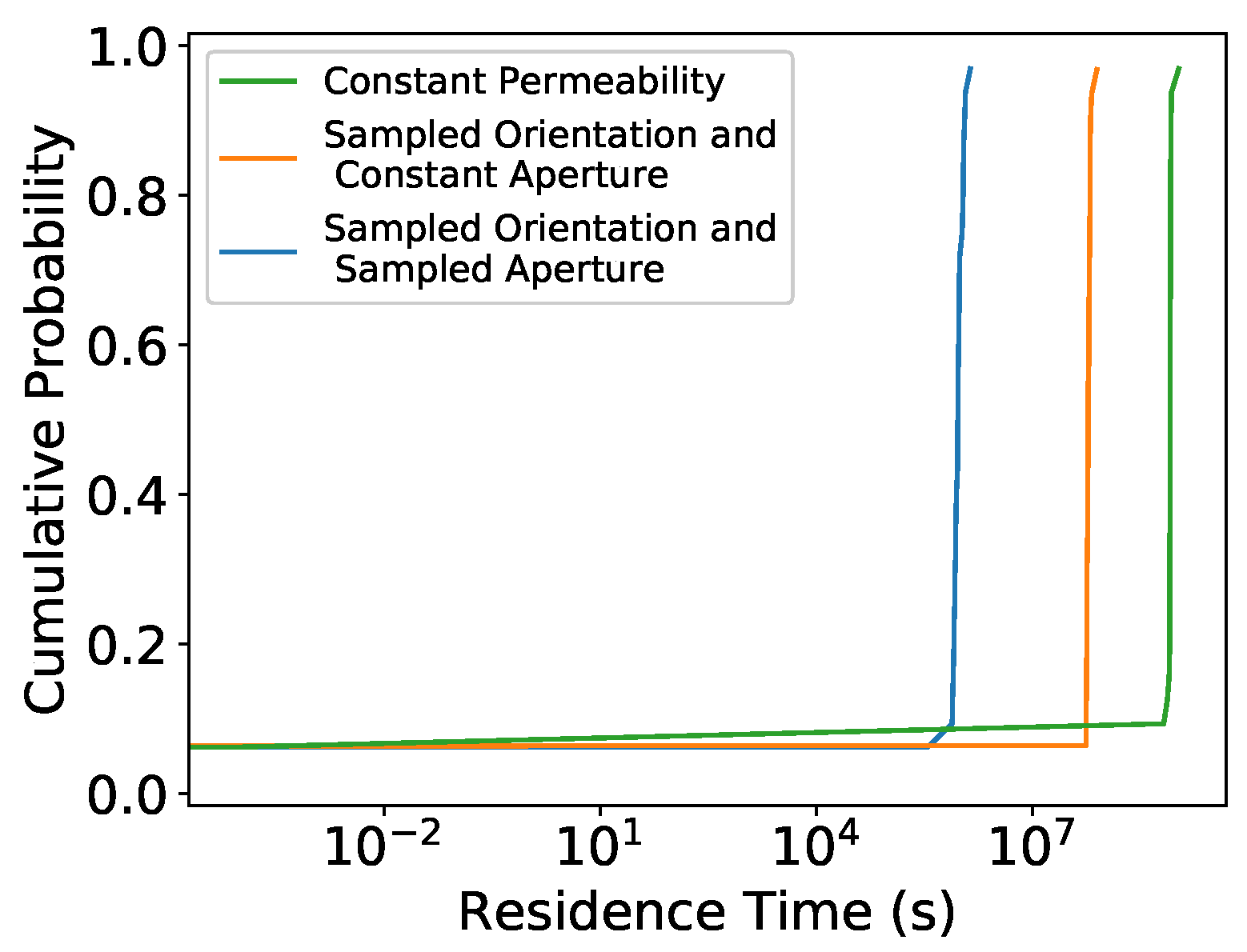
Figure 10.
The cumulative distribution of the fluid residence time based on the seepage velocity distribution for the constant permeability, constant aperture, and sampled aperture cases shown in Figure 8. Preferential flow paths arising from the fracture heterogeneity greatly impact the fluid residence times—significantly reducing them compared to the assumption of an average permeability.

Publisher’s Note: MDPI stays neutral with regard to jurisdictional claims in published maps and institutional affiliations. |
© 2021 by the authors. Licensee MDPI, Basel, Switzerland. This article is an open access article distributed under the terms and conditions of the Creative Commons Attribution (CC BY) license (https://creativecommons.org/licenses/by/4.0/).
Share and Cite
MDPI and ACS Style
Hu, R.; Walsh, S.D.C. Effective Continuum Approximations for Permeability in Brown-Coal and Other Large-Scale Fractured Media. Geosciences 2021, 11, 511. https://0-doi-org.brum.beds.ac.uk/10.3390/geosciences11120511
AMA Style
Hu R, Walsh SDC. Effective Continuum Approximations for Permeability in Brown-Coal and Other Large-Scale Fractured Media. Geosciences. 2021; 11(12):511. https://0-doi-org.brum.beds.ac.uk/10.3390/geosciences11120511
Chicago/Turabian StyleHu, Roger, and Stuart D. C. Walsh. 2021. "Effective Continuum Approximations for Permeability in Brown-Coal and Other Large-Scale Fractured Media" Geosciences 11, no. 12: 511. https://0-doi-org.brum.beds.ac.uk/10.3390/geosciences11120511
Note that from the first issue of 2016, this journal uses article numbers instead of page numbers. See further details here.