
An Open-Source Code for Fluid Flow Simulations in Unconventional Fractured Reservoirs


1
Craft and Hawkins Department of Petroleum Engineering, Louisiana State University, Baton Rouge, LA 70803, USA
2
Dipartimento di Ingegneria dell’Innovazione, Università del Salento, 73100 Lecce, Italy
*
Author to whom correspondence should be addressed.
Geosciences 2021, 11(2), 106; https://0-doi-org.brum.beds.ac.uk/10.3390/geosciences11020106
Submission received: 5 January 2021
/
Revised: 4 February 2021
/
Accepted: 12 February 2021
/
Published: 22 February 2021
(This article belongs to the Special Issue Quantitative Fractured Rock Hydrology)
Abstract
:In this article, an open-source code for the simulation of fluid flow, including adsorption, transport, and indirect hydromechanical coupling in unconventional fractured reservoirs is described. The code leverages cutting-edge numerical modeling capabilities like automatic differentiation, stochastic fracture modeling, multicontinuum modeling, and discrete fracture models. In the fluid mass balance equation, specific physical mechanisms, unique to organic-rich source rocks, are included, like an adsorption isotherm, a dynamic permeability-correction function, and an Embedded Discrete Fracture Model (EDFM) with fracture-to-well connectivity. The code is validated against an industrial simulator and applied for a study of the performance of the Barnett shale reservoir, where adsorption, gas slippage, diffusion, indirect hydromechanical coupling, and propped fractures are considered. It is the first open-source code available to facilitate the modeling and production optimization of fractured shale-gas reservoirs. The modular design also facilitates rapid prototyping and demonstration of new models. This article also contains a quantitative analysis of the accuracy and limitations of EDFM for gas production simulation in unconventional fractured reservoirs.
1. Introduction
Unconventional gas reservoirs are gaining interest as decades of oil and natural gas production have resulted in extensive use of conventional resources. As a consequence, new technologies, like horizontal well drilling and hydraulic fracturing, are constantly being introduced, driving substantial growth of the production of these unconventional resources [1].
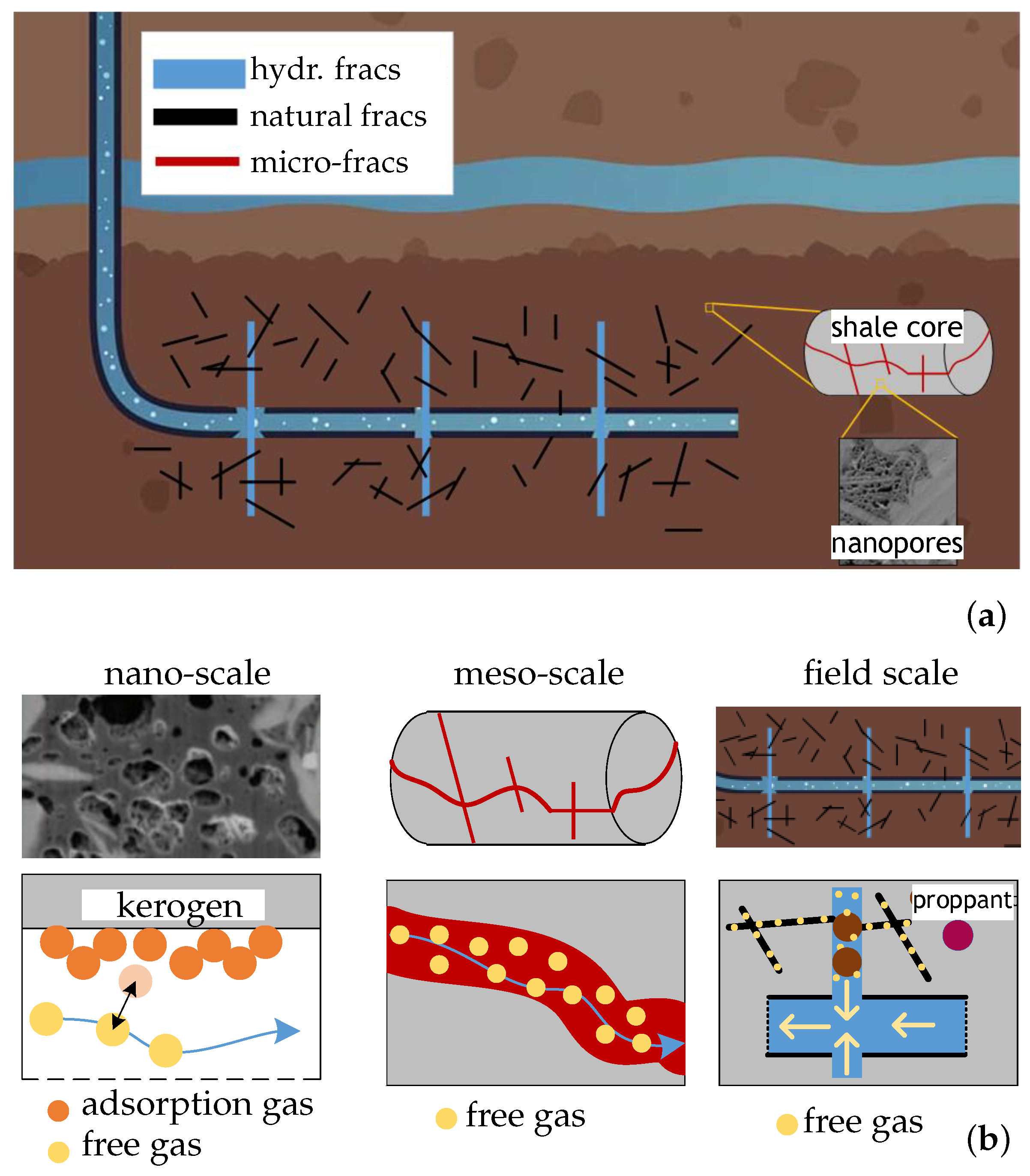
The exploitation of such resources is technologically demanding and expensive. There is a need for high-quality predictive models for more efficient and economic design and management of the production process. Unlike the conventional reservoirs, unconventional reservoirs are characterized by complex transport mechanism and the occurrence of multiscale fractures [2], therefore, the well-established models for flow and transport in porous media are not usable [3]. In fact, with specific reference to fractured shale, the rock mass is comprised of a matrix of dense, tiny pores of sizes down to a few nanometers, cracks, and microfractures, giving intrinsic heterogeneity and anisotropy [2,4], and superposed natural/artificial long or relatively long fractures; given these features, an accurate and reliable prediction of a well’s performance is challenging (Figure 1).
The methods proposed in the scientific literature for the prediction of gas flow in such reservoirs can be categorized into analytical, semianalytical, and numerical. The analytical methods date back to the 70s; solutions of the linearized real-gas equation were derived for simple fracture geometries [5,6]. The semianalytical methods were based on the Boundary Element Method (BEM) and found to be effective for more complex fracture networks and shale gas storage, including adsorption [7,8,9,10,11,12,13,14,15]. Although the analytical or semianalytical methods are, when applicable, fast and accurate, the numerical methods are generally preferred [15,16]. Discrete Fracture Networks (DFNs) are frequently used as geometrical/hydromechanical input for simulations of fluid flow in fractured rock masses that have multiscale fractures [17]. Usually, the DFN is limited to the larger features and is embedded into a continuum of given hydraulic properties, condensing the matrix and the network of cracks and tiny fractures [18,19].
The coupling of the DFN mesh with the continuum mesh is crucial, and unstructured meshing/gridding with Local Grid Refinement (LGR) is generally used, however, the operation is challenging, especially when dealing with intricate DFNs. With a conforming mesh, it may be difficult to efficiently simulate the sharp pressure gradients around the fractures [20]. In order to resolve such a problem, the Embedded Discrete Fracture Model (EDFM) has been recently proposed. In an EDFM, the DFN is embedded into the continuum (matrix, cracks and tiny fractures) without conforming the meshes. A structured mesh/grid is employed for the continuum; the required precision can be comfortably reached by reducing the element size. In addition, an EDFM can be easily incorporated in existing, well-established reservoir simulators [15]. In Table 1, the EDFM is compared to other methods for the simulation of gas transport in unconventional reservoirs. EDFM has been widely adopted for gas production simulation in unconventional fractured reservoirs by considering various flow mechanisms and models [21,22,23,24,25].
To the authors’ knowledge, almost all the existing codes for shale gas reservoirs are implemented in in-house simulators or commercial simulators [2]. As a better understanding of the flow mechanisms in unconventional reservoirs is gained, many emerging flow models and technologies will be developed for the effective development of unconventional reservoirs [26,27,28,29]. However, the prediction of gas transport in shale is still a hard task considering the complexity of the involved phenomena, specifically with reference to the well performance; in this respect, more flexible and open-source tools may be useful to the scientific collective for better understanding and rapid prototyping and demonstration of new simulation models. Further, although EDFM is an efficient method to solve the fluid flow problem in fractured reservoirs, Tene et al. [30] show that it may introduce large errors when dealing with low conductivity or sealing faults/fractures. The effect of such errors on the prediction of well performance is hard to define.
In this note, a numerical code (ShOpen) for the simulation of nonlinear gas flow in unconventional reservoirs with multiscale fractures is described. It is an efficient and flexible framework (ShOpen) including the MATLAB Reservoir Simulation Toolbox (MRST), an open-source reservoir simulation toolkit, and an EDFM. ShOpen can handle discrete hydraulic fractures of arbitrary geometry and location. The code also encompasses the geomechanical effects on the fractures of the DFN. The typical results of the code are compared to those of a commercial simulator and of an in-house reservoir simulator, employing unstructured grids to simulate gas desorption, gas slippage, and diffusion in shale with nonplanar hydraulic fractures. The advantages and limitations of EDFM in predicting the well performance of unconventional reservoirs are then discussed. Finally, some practical applications are reported.
The note is structured as follows: the physicomathematical statements underpinning the code and the numerical model are described in Section 2 and Section 3, respectively. In Section 4, the validation of the code is reported; in Section 5, the practical examples of application are illustrated; in Section 6, concluding remarks are provided.
2. Physicomathematical Statements
A domain dense of a porous matrix is crossed by fractures of a domain . In two dimensions (plane flow), the equations ruling the isothermal single-component single-phase gas flow in both and is as follows [31]:
where is equal to ‘m’ or ‘f’ for matrix and fracture, respectively; t is time; b is inverse formation volume factor, equal to the ratio , with , gas densities at the reservoir conditions and at standard conditions, respectively; is porosity; is gas mass adsorption (negligible for the fracture); is the permeability correction factor for the i-th gas transport mechanism; is the absolute permeability; is the gas dynamic viscosity; is pressure; q is gas volumetric sink/source; and is the leakage term between the two domains (). The permeability derives from the initial absolute permeability after correction by using factors , , , (i.e., ), condensing, respectively, the effects of slippage and diffusion, deviation from Darcy law and indirect hydromechanical coupling, and for micro/meso-cracks/fractures embedded into , for discrete fractures.
Note that in Equation (1), the gravity is neglected.
In what follows, the terms of Equation (1) are explicated.
2.1. Gas Density
For the density of a natural gas, modified ideal gas law applies:
where p is gas pressure (irrespective of the domain); M is the gas molar mass; R is the ideal gas constant (8.314 JKmol); T is the reservoir temperature; and Z is the compressibility factor, a function of p and T.
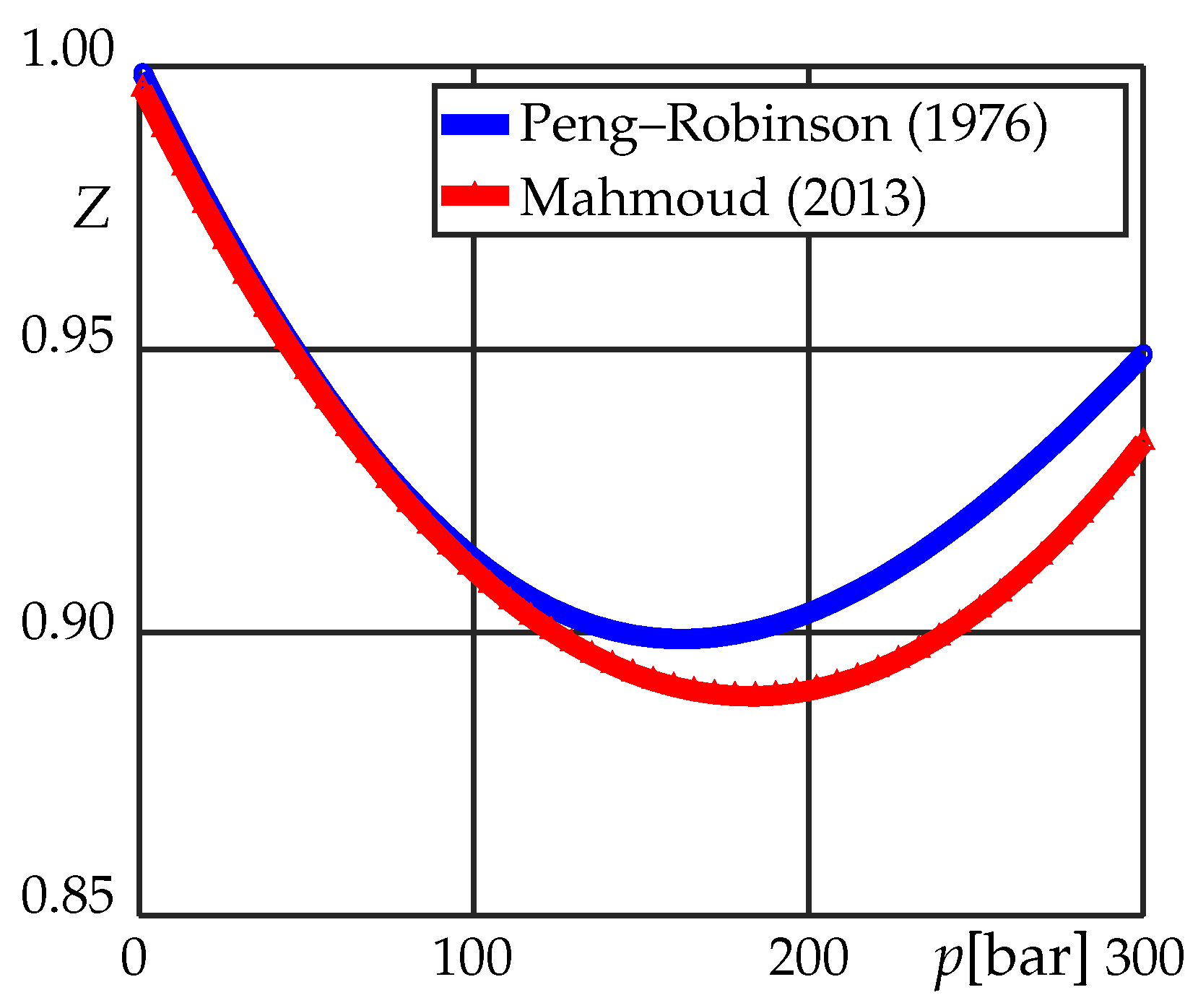
For factor Z, the implicit Peng–Robinson Equation-Of-State (PR-EOS) [32] can be used, or, alternatively, empirical explicit equations can be applied. Elliot and Lira [33] propose for Z a cubic equation:
whose coefficients are as follows: , , , with and , where is the acentric factor for the species; is the pseudo-reduced pressure; and is the pseudo-reduced temperature, respectively, equal to and , where and are the pseudo-critical pressure and pseudo-critical temperature of a natural gas. The pseudo-critical values are weighted averages (by considering the molar fractions) of the critical values of the gases constituting the mixture.
Mahmoud (2013) [34] instead provides the following equation:
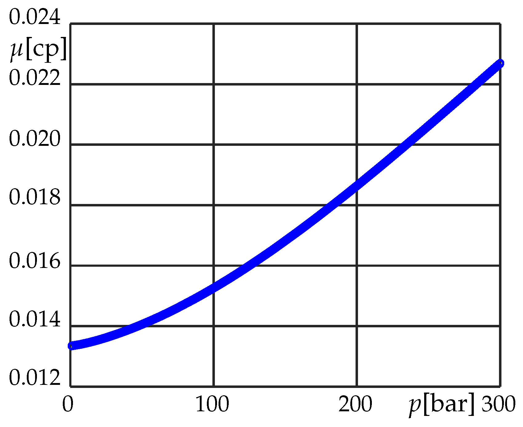
2.2. Gas Viscosity
2.3. Adsorption and Transport
With the development of unconventional tight reservoirs in recent years, enormous effort has been spent to simulate gas adsorption and transport in shale (Figure 1). The related mechanisms and corresponding models [36,37,38,39,40,41] are summarized in Table 2, with indications of the relative domain of application (matrix or fracture).
In ShOpen, all the adsorption and transport models of Table 2 can be easily implemented by introducing the corresponding formulations for the nonlinear gas adsorption and the permeability correction functions . In what follows, examples of the models implemented in ShOpen are described.
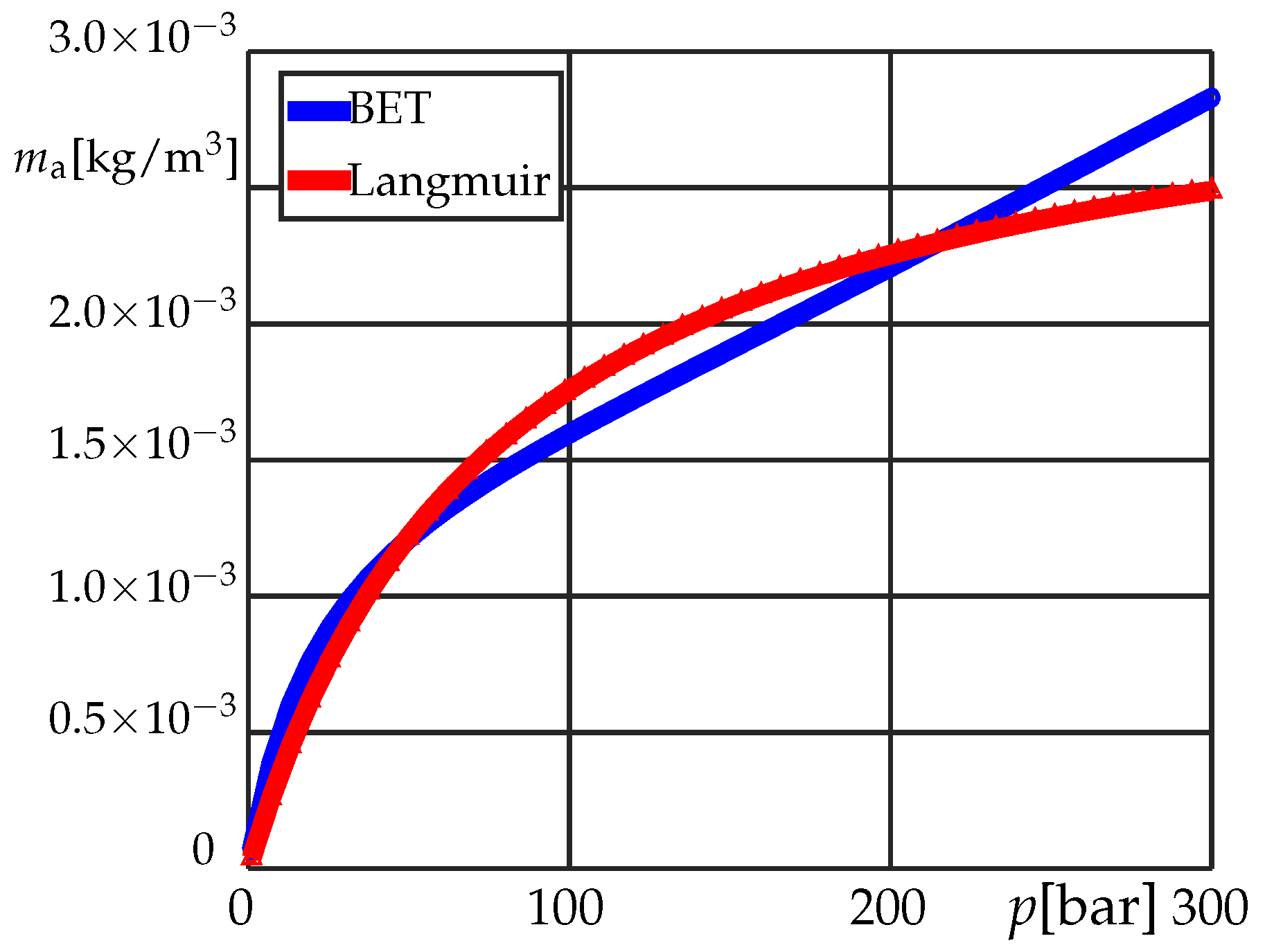
For the adsorption, the amount of gas molecules adsorbed in the pore wall of Kerogen in shale reservoir can be estimated by using a monolayer Langmuir isotherm and a multilayer BET isotherm. In formula, respectively [40]:
where is the Langmuir volume, i.e., the maximum adsorbed gas volume at a given temperature for an infinite pressure; is the Langmuir pressure, i.e., the pressure at which the adsorbed gas volume is equal to /2; is the bulk density of the rock matrix (rock density in what follows); is the BET adsorption volume; C is the BET adsorption constant; n is the number of adsorption layers; is the reduced pressure, equal to ; and is the BET pseudo-saturation pressure, equal to .
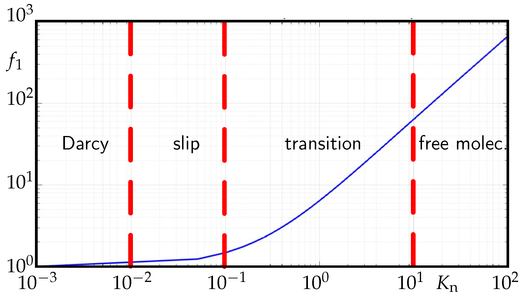
For the effect of slippage flow and diffusion, the permeability in the low-pressure regions around the fractures increases. In ShOpen, the correction factor of Florence et al. [37] is implemented. In formula:
where is the Knudsen number, equal to
and is the rarefaction parameter, equal to
2.4. Indirect Hydromechanical Coupling
As shown in Figure 1b, a shale reservoir may have multiscale fractures. The fracture conductivity may decrease/increase with the production time for the closing/opening of the fracture in the near field of a well. The effect descends from the so-called indirect hydromechanical coupling. Specifically, the pumping/injection-induced pressure change in a fracture gives rise to a corresponding normal effective stress change that, in turn, drives to a normal deformation of the fracture and a change of the conductivity [2,45,46,47,48]. The effect can be properly estimated by resorting to full simulations of the hydromechanical coupling, where both fluid flow and stress/strain regime are included [49,50]. However, under the assumption of total stresses unchanged (), the decoupling can be applied, thus, and relations for the correction of the fracture permeability can be easily applied. So, a fully hydromechanically coupled solution is not pursued, rather, these relations are introduced to incorporate the effect of effective stress changes on the fluid flow.
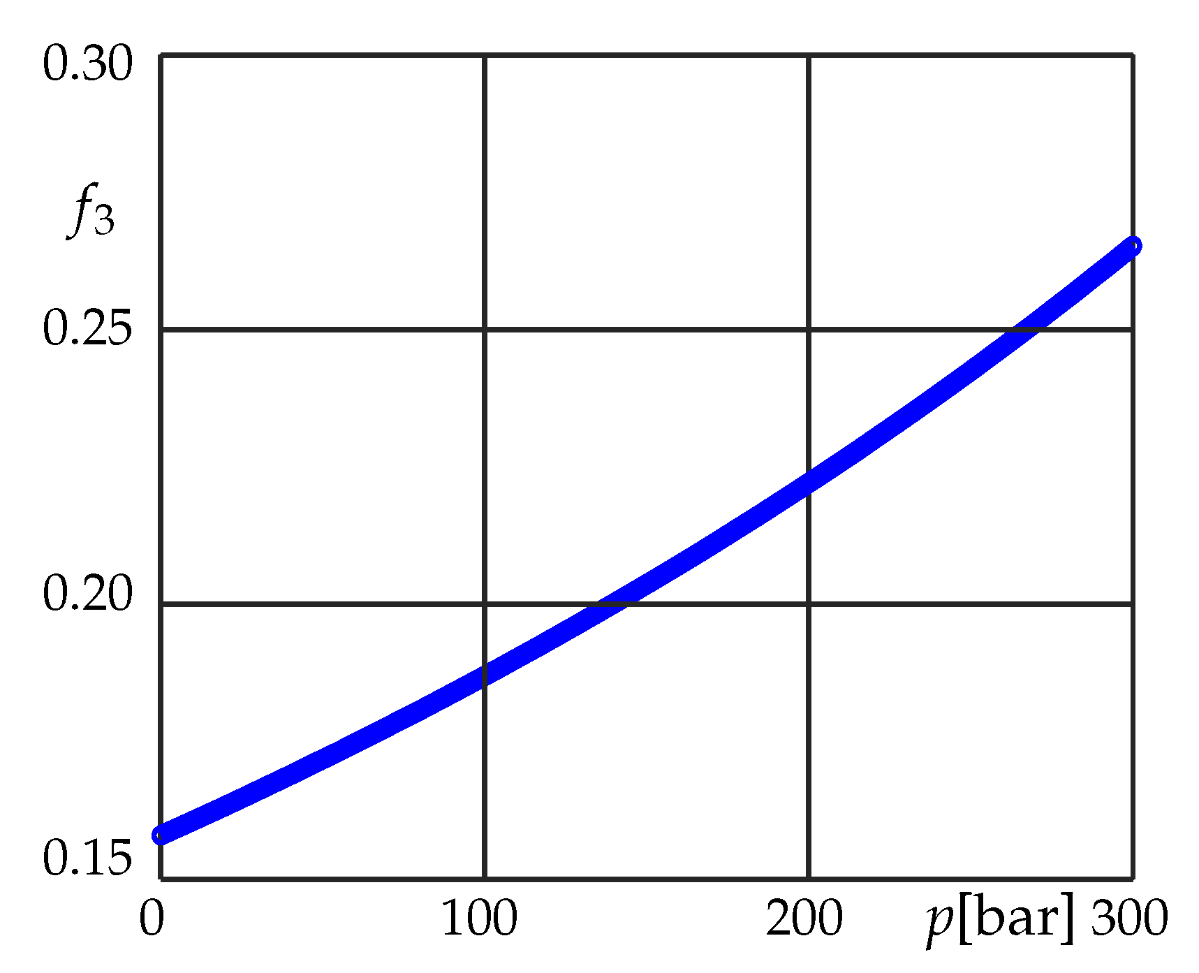
For micro/meso-cracks/fractures, a correction factor is furnished by Gangi [51]:
where is the normal (with respect to the mean plane of the fracture) effective stress; is the effective modulus of the asperities, which is equal to the rock modulus multiplied by the ratio of the area of the asperities and fracture area (from one-tenth to one-hundredth of the rock bulk modulus); and m is related to roughness of the fracture walls. The stress is defined as , where is the total normal stress and is the Biot coefficient for a fracture. In this work, we assume the vertical overburden stress is the total normal stress applied to fractured rocks.
In Figure 6, an estimation of by using Equation (13) is reported using the value suggested by [52] for unconventional rock samples.
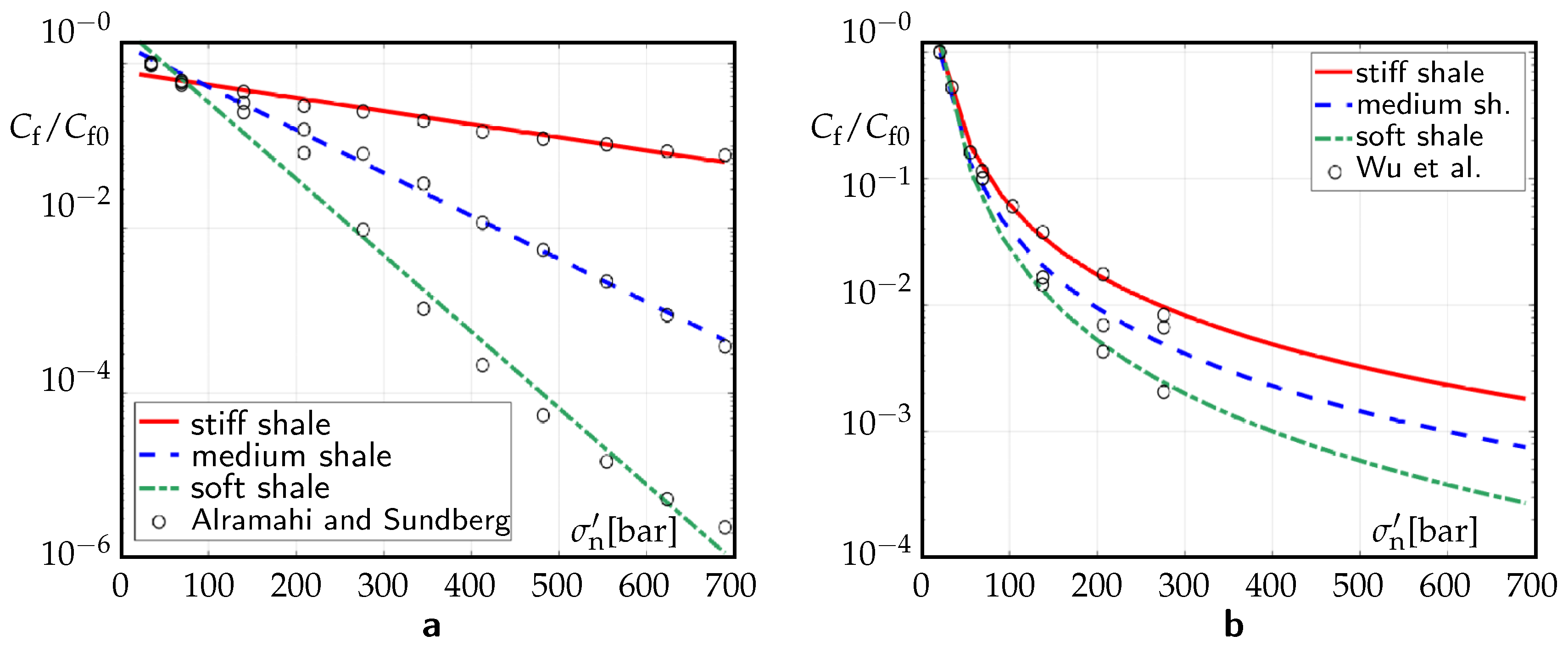
For propped fractures, Alramahi and Sundberg (2012) [53] performed a series of experiments to measure the effect of the normal (to the fracture plane) effective stress on the conductivity of fractures in shale having different stiffness (fracture conductivity is the product of the fracture permeability with the fracture width w, unit md-ft). The authors reported an empirical relationship of the type:
where the units of , are md-ft and psia, respectively, and , are coefficients related to the stiffness of the shale as follows: stiff shale: −0.00011, −0.0971; medium shale: −0.00035, 0.2396; soft shale: −0.00064, −0.4585.
Wu et al. (2019) [54] performed similar experiments on unpropped fractures. The type of the derived relations is
where the units of , are again md-ft and psia, respectively, and coefficients , are as follows: stiff shale: −0.793, 4.5618; medium shale: −0.89, 5.0725; soft shale: −1.04, 6.0216.
In Figure 7, , normalized to the initial value of , is plotted against for propped and unpropped fractures.
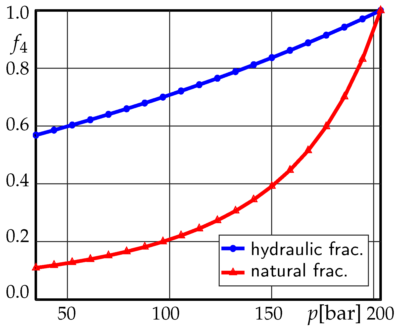
In case of an artificial (hydraulic, H) fracture, the direction of propagation is normal to the minimum total horizontal stress . The orientations of a natural (N) fracture is instead random, even though they cluster around the mean values pertaining to the fracture sets. The total normal stress on a fracture can be approximated by the average total normal stress. Therefore, can be defined as follows, respectively:
where may coincide with horizontal stresses at the site if the fractures are supposed to be oriented sub-vertically. Note that is set to 1.
In ShOpen, a dynamical correction factor for H and N fracture permeabilities is introduced:
where is the initial reservoir pressure.
Typical trends of the correction factor versus p for both H and N fractures are reported in Figure 8.
In ShOpen, the three categories of fractures, i.e., micro/meso-cracks/fractures, N fractures, and H fractures, are defined according to length and aperture as follows, respectively: /2 < 1 m, < 0.1 mm; /2 = 1–20 m, = 0.1–1 mm; /2 = 20–100 m, > 1 mm.
3. The Numerical Model
ShOpen includes the following modules: the automatic differentiation module (ad-core, ad-props), the black-oil module (ad-blackoil), and the hierarchical fracture model (hfm), implemented into the open-source MATLAB Reservoir Simulation Toolbox (MRST) [55]. The Two-Point-Flux Approximated Finite Volume Method (TPFA-FVM) is applied for the solution of the governing Equations (1). A fully implicit first-order backward scheme is applied for the time discretization, in which the Jacobian matrix of the nonlinear system is calculated by the automatic differentiation modules. All the nonlinear functions for adsorption, transport, and hydromechanically coupled effects are separately handled. The large H and N fractures are explicitly modeled. The micro/meso-crack/fractures are embedded into the matrix.
3.1. Numerical Discretization
By using an implicit scheme and backward finite differences, and by subdividing in cells of volume V, Equation (1) can be expressed as follows:
where there is no mechanical storage and is factored out of the temporal derivative. In a two-dimensional Cartesian mesh with uniform formation thickness h, the cell volume is defined as , with A cell area.
The leakage terms are coupling terms (as illustrated later), therefore, for both domains in Equation (18), and coexists. The matrix form of Equation (18) is as follows:
where and condense the gas volumetric sources/sinks.
Note that the correction factors all depend on . In order to handle the nonlinearities of Equation (19), Newton’s iteration method is used. The residual function of variables at each iteration n can be expressed as follows:
where the Jacobian matrix , equal to , is calculated by automatic differentiation in MRST.
3.2. EDFM
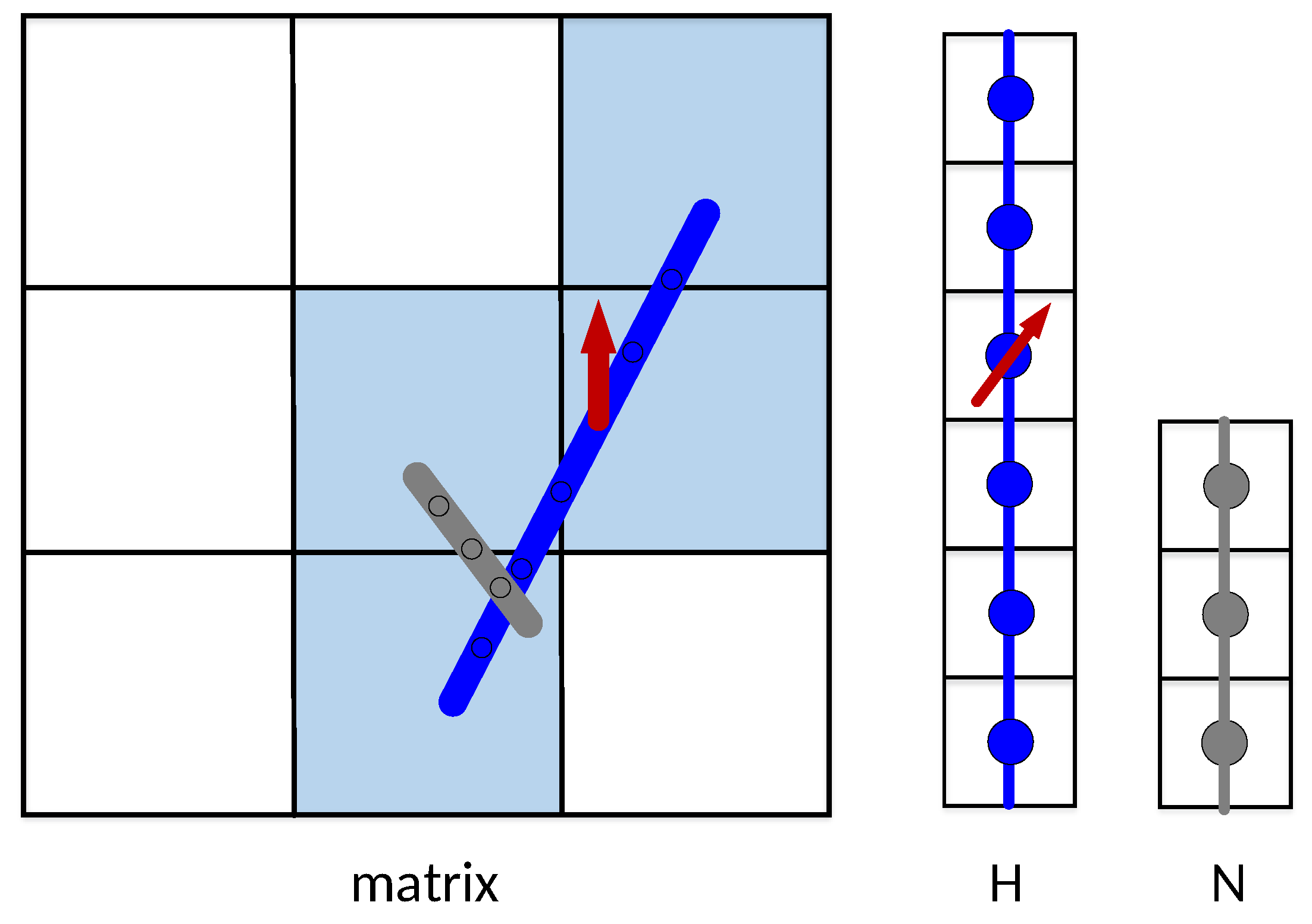
As shown in Figure 9, in an EFDM, the matrix mesh is not necessarily conforming with the fracture elements. There are three Non-Neighbor Connections (NNCs) in an EDFM: (1) fracture–matrix, (2) fracture–fracture, (3) fracture–well. For a fracture–matrix NNC, the following equation applies [56]:
where is a fracture-to-matrix transfer coefficient. Being that i is a node of the matrix mesh/grid and k is a neighbor node of a fracture intersecting the cell of i, the transfer coefficient is
where is the area of the intersection between the fracture and grid cell. For a 2D grid, is the product of the linear intersection with the uniform formation thickness . Note that the harmonic average and upwind scheme are used for the permeability and viscosity, respectively. The quantity is the volumetric averaging normal distance between matrix cell and fracture plane, which can be calculated as follows:
For two-dimensional structured grids, an analytical solution is available for [57].
For fracture–fracture NNC, star–delta transformation is used to compute the fracture–fracture transfer coefficient for a fracture intersection [58]:
where is a transfer coefficient for a fracture cell m in a fracture intersection; is the cross-section area of the fracture in m, which can be calculated by multiplying the fracture aperture with the formation thickness ; is the fracture cell length in m; and is the total number of fracture–fracture connections.
For a fracture–well NNC, the effective wellbore index between a fracture cell and a well and the equivalent radius can be expressed, respectively, as follows [56]:
where s is the wellbore skin factor.
4. Validation
For the validation of ShOpen, the results of numerical simulations for a methane (CH) reservoir are compared to the results furnished by the CMG© simulator (Computer Modelling Group Ltd., Calgary, AB, Canada, www.cmgl.ca (accessed on 23 February 2021)) (validation examples VE1A, VE1B, VE1C) and an in-house simulator with unstructured mesh (validation example VE2) [59]. For the simulations, the following data are fixed: rock density 2500 kg/m; CH molecular weight, critical pressure, critical temperature, acentric factor are, respectively, 0.01604 kg/mol, 4.60 MPa, 190.6 K, 0.01142, well radius 0.1 m.
4.1. Comparison with the Commercial Simulator
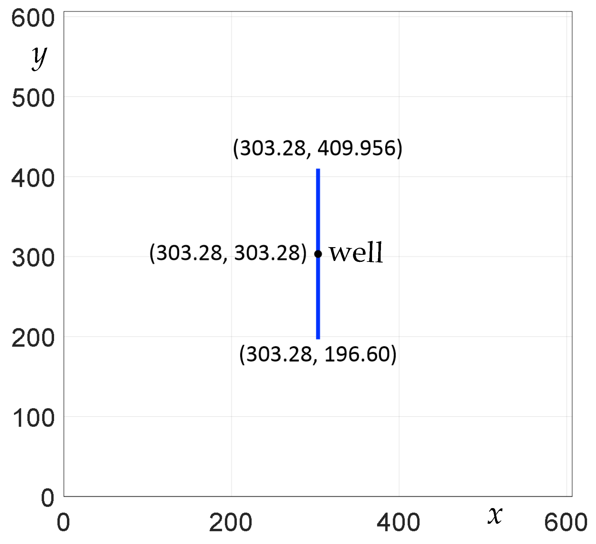
With reference to Figure 10, the size of the reservoir domain is 606.6 × 606.6 m. A well is located at the center of a 200 m-long hydraulic fracture parallel to the y axis. As the commercial simulator does not support all the physics presented in Section 2, only the Langmuir adsorption (Equation (6)) is considered. Compressibility factor Z and natural gas viscosity values are derived through interpolation of the values suggested in CMG©. Specific input data are reported in Table 3. For the well, the bottom-hole pressure (BHP) is given. The production time is 30 years. The domain is discretized with 201 and 65 cells.
EDFM is an efficient method to solve fluid flow problem in fractured reservoirs, however, Tene et al. [30] show that it may introduce large errors when dealing with low-conductivity or sealing faults/fractures. Additionally, LGR is usually required to capture the sharp pressure gradients near the fractures. To evaluate the performance of EDFM method for practical shale gas production problem, three simulation scenarios (VE1A, VE1B, and VE1C) are performed.
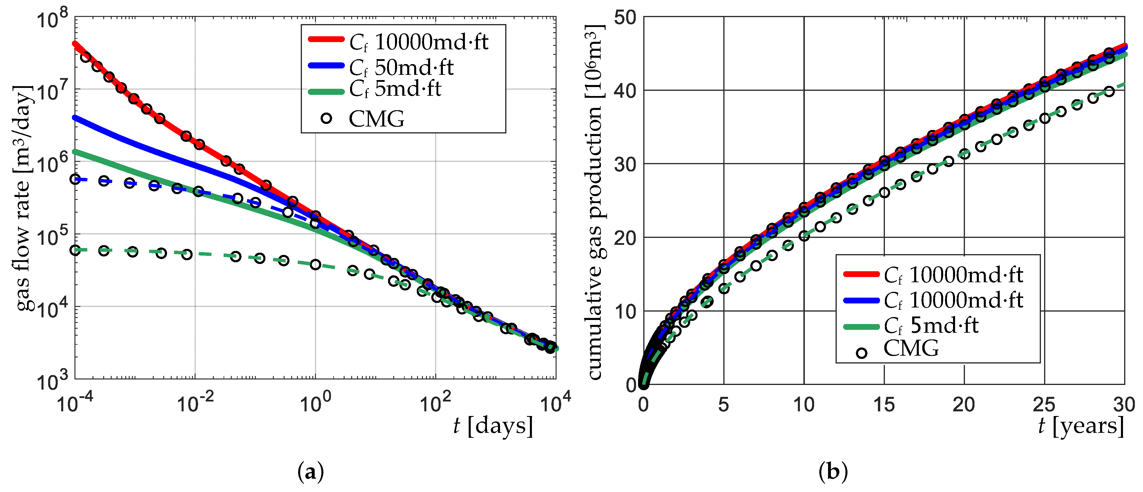
In VE1A, three scenarios with fracture conductivity equal to 10,000 mD-ft, 50 mD-ft, and 5 mD-ft, respectively, are simulated. In Figure 11, the results in terms of gas flow rate and cumulative production are plotted against time for ShOpen (EDFM and explicit EFM) and CMG.
The results of ShOpen/EFM are in good agreement with the results provided by CMG, whereas the results of ShOpen/EDFM consistently deviate with a significant difference of even 11%. It is apparent that the production in a reservoir with fractures of low to medium permeability cannot be efficiently simulated with EDFM, as previously stated by Tene et al. (2017) [30].
For unconventional reservoir simulations, LGR is usually required to capture the sharp pressure gradients near the fractures. In VE1B, the sensitivity of the solution provided by both ShOpen/EDFM and ShOpen/EFM to the type of grid is explored.
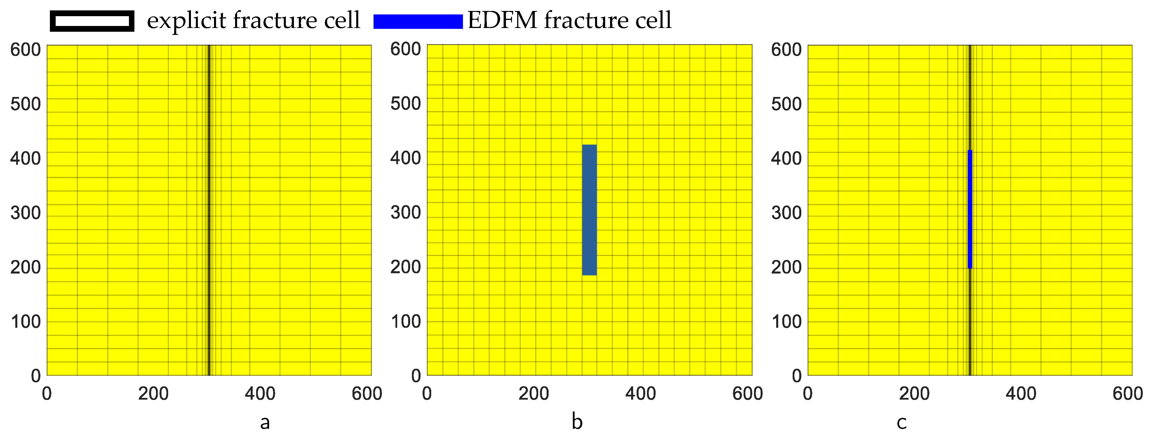
With reference to Figure 12, the three grid types are LGR with logarithmic refinement; a standard uniform EDFM grid [30]; and a combined EDFM + LGR grid, with an additional EDFM fracture cell superposed to the LGR grid. Note that the number of all cells is equal for all the grids (499 × 61).
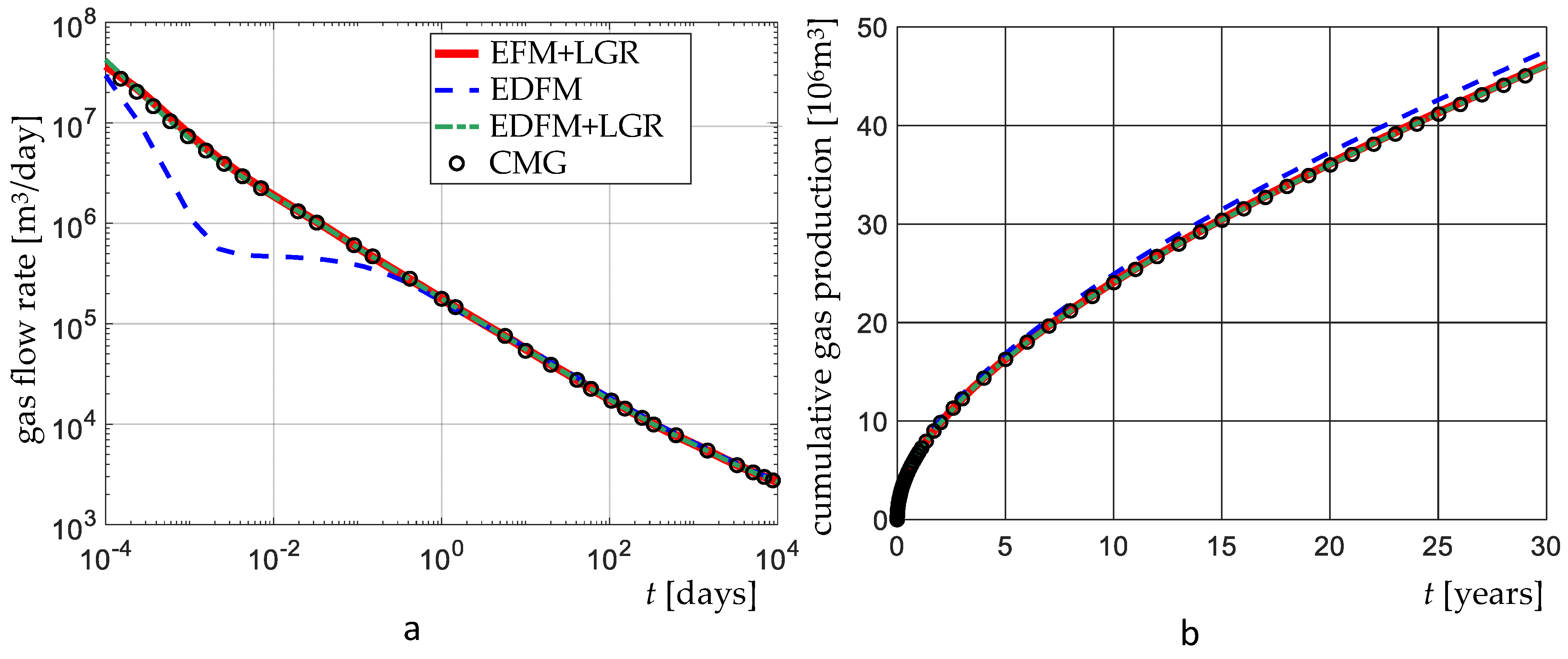
Fracture conductivity is set to 10,000 mD-ft. All other parameters are maintained equal to VE1A. The results are compared to the results offered by CMG. In Figure 13 and Figure 14, it is shown that the results in terms of gas flow rate and cumulative gas production provided by ShOpen are in good agreement with the results of CMG. Again, with ShOpen/EFM, the obtained results match with those of CMG, whereas with ShOpen/EDFM, a 3.3% difference for the cumulative gas production is experienced. It is demonstrated therefore that EDFM can capture the sharp pressure gradient near a fracture only when LGR is applied.
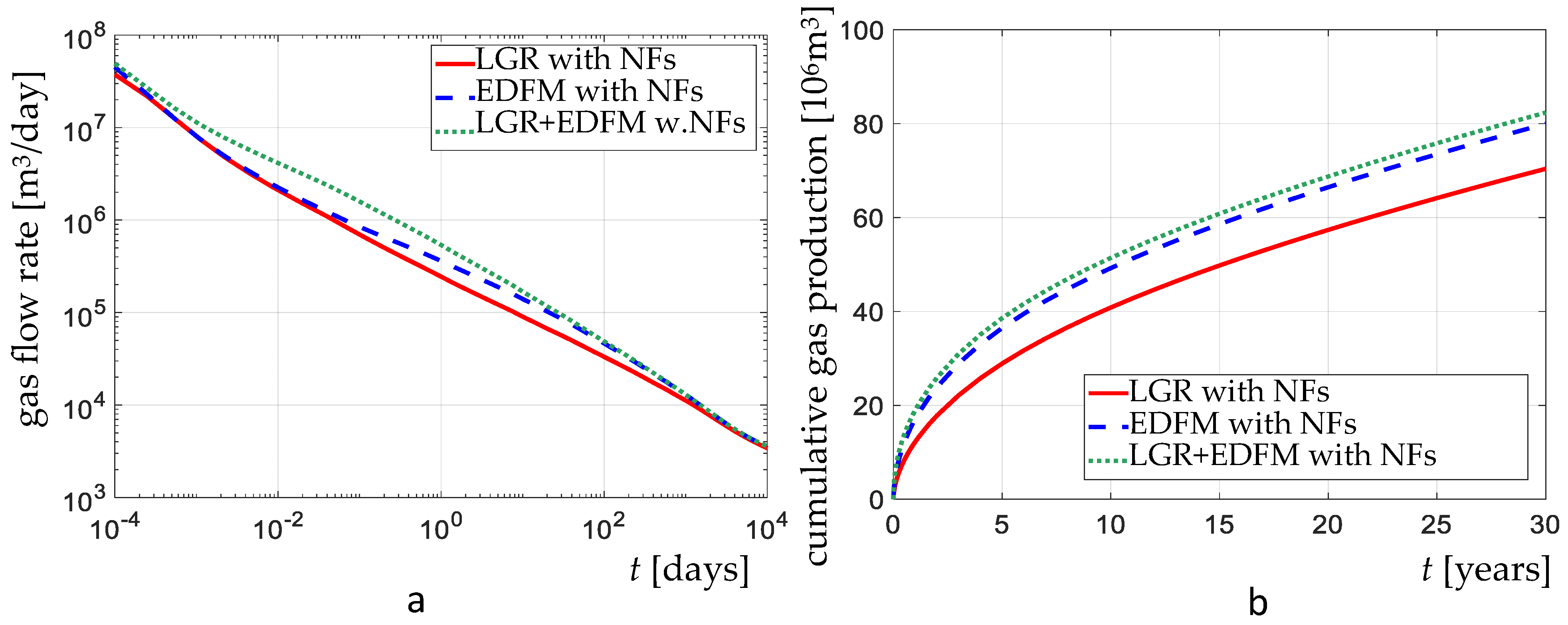
In consideration of the abovementioned, in VE1C, the effect of grid refinement of fractures on the accuracy of the solution for ShOpen/EDFM is also investigated. With reference to Figure 15, six 116.74 m-long natural fractures are added in the domain; the grids of the fractures are built with and without resorting to LGR. The fracture conductivity of these fractures is 5 mD-ft, whereas it is kept to 10,000 mD-ft in one of the hydraulic fractures.
In Figure 16, it is shown that by using ShOpen/EDFM, a significant difference (almost 17%) with respect to CMG results is obtained. Furthermore, an underestimation of the well performance by using EDFM without LGR is experienced (3.4% difference). Again, it is further demonstrated that EDFM without LGR is not adequate for modeling reservoir models with low-permeability fractures.
To sum up, EDFM, without LGR, converges to the reference solution only when fracture conductivities are very high. In practical cases, it could be misleading to assume that all the natural fractures or faults have high permeability values, given that many of these features may be no longer active under the existing stress state in the rock of the reservoir. The use of LGR and an improved EDFM algorithm [30] for handling low-permeability fractures in the context of EDFM are all but mandatory. To relieve the limitations of EDFM in the following simulations, an empirical skin-factor and uniform grid refinement are adopted.
4.2. Comparison with an In-House Simulator
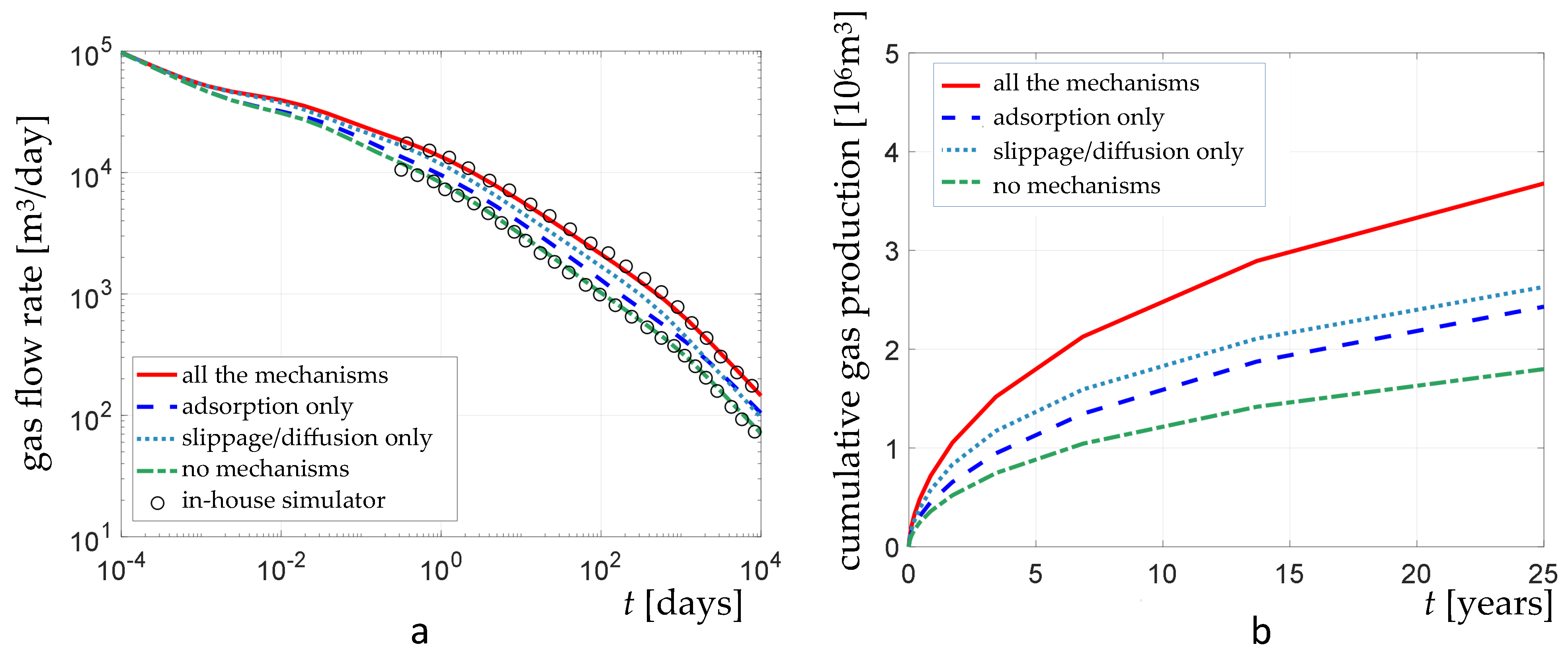
ShOpen is further validated by comparing the results with those provided by an in-house simulator [59], with reference to a reservoir with a complex networks of embedded fractures (simulation VE2). For the simulation, an unstructured mesh with LGR is used for capturing the sharp pressure gradients near the fractures. The performance of a well is considered in a reservoir with a simple “regular” fracture network (Figure 17). To reproduce the results in [59], adsorption (Equation (6)) and slippage/diffusion effects (Equation (8)) are considered in this example. With reference to the adsorption and transport mechanisms, four scenarios are considered: with adsorption and slippage/diffusion, adsorption only, slippage/diffusion only, and no mechanisms. The input data for VE2 are reported in Table 4. The production time is 10,000 days.
In Figure 18, the simulated gas flow rate and cumulative gas production are reported for both ShOpen and the in-house simulator, and for the considered scenarios. The results provided by the two codes match almost perfectly.
5. Application Examples
In order to illustrate the applicability of ShOpen to practical problems, two of the unconventional reservoirs with complex fracture networks are simulated (simulations AE1 and AE2) and the relative results presented.
5.1. Barnett Shale Reservoir
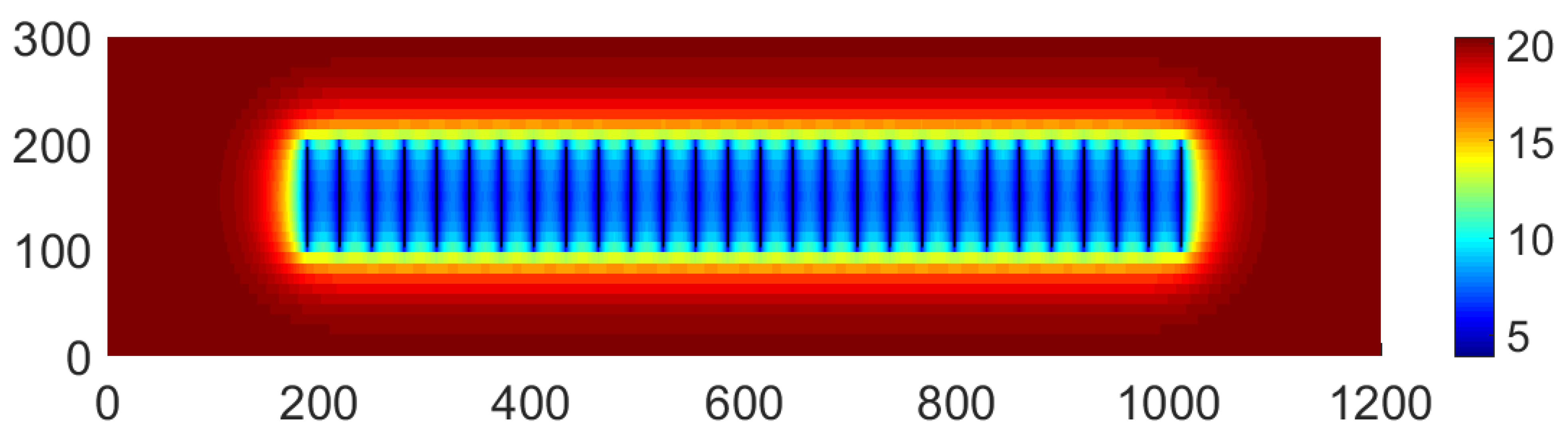
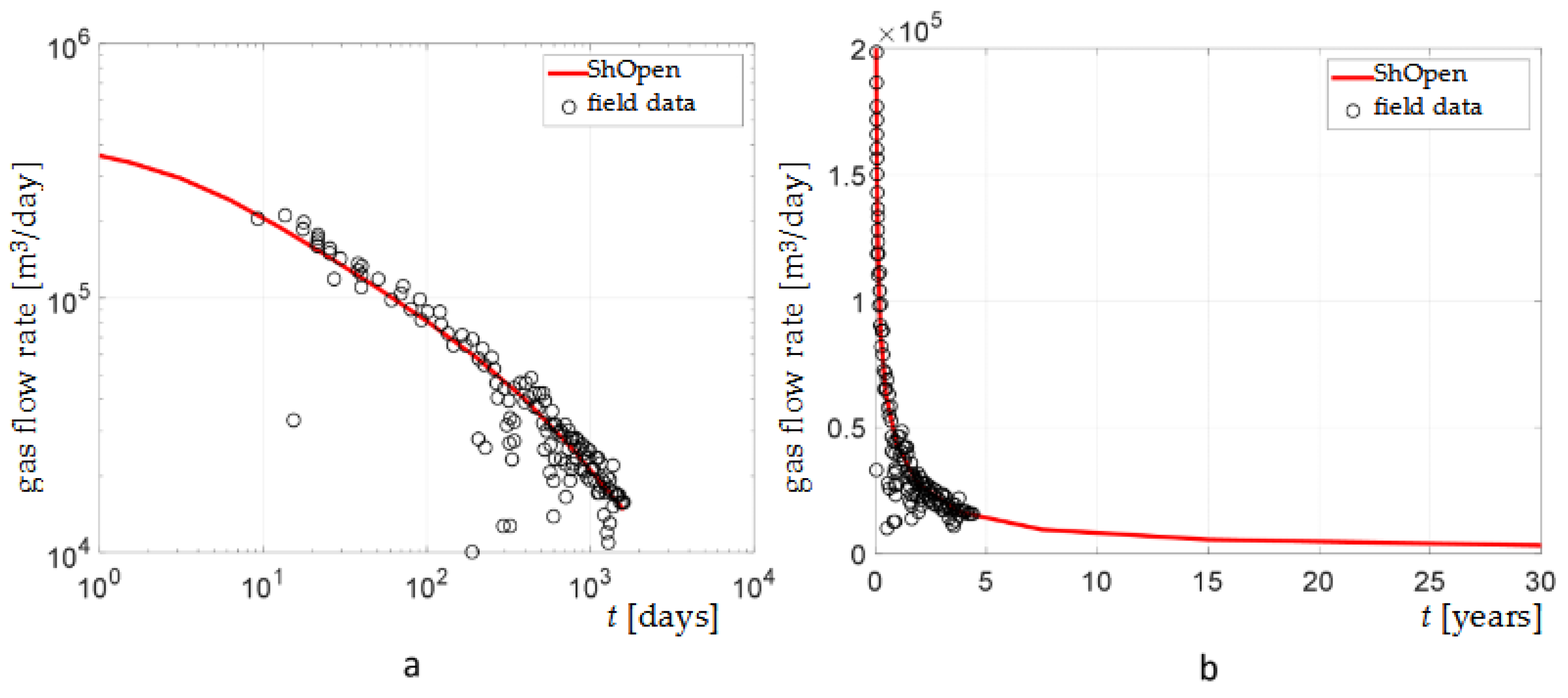
The history of the field production data of the Barnett shale reservoir is simulated with Shopen (simulation AE1). The input data are excerpted from the literature [60] and reported in Table 5. The scheme of the simulation and the mesh are shown in Figure 19. A 1100 × 290 m rectangular reservoir with a thickness of 90 m is discretized by using 148 × 39 cells. Twenty-eight 94.4 m-long parallel H fractures are situated in the middle. The mutual spacing is 30.5 m. The fractures all have an aperture of 0.003 m and a permeability of 100 mD. Langmuir adsorption (Equation (6)) is considered. The depth of the reservoir is 5463 m.
In Figure 20, the pressure contours, derived from the ShOpen simulation, after 1600 days are shown.
5.2. Reservoir with a Stochastic DFN
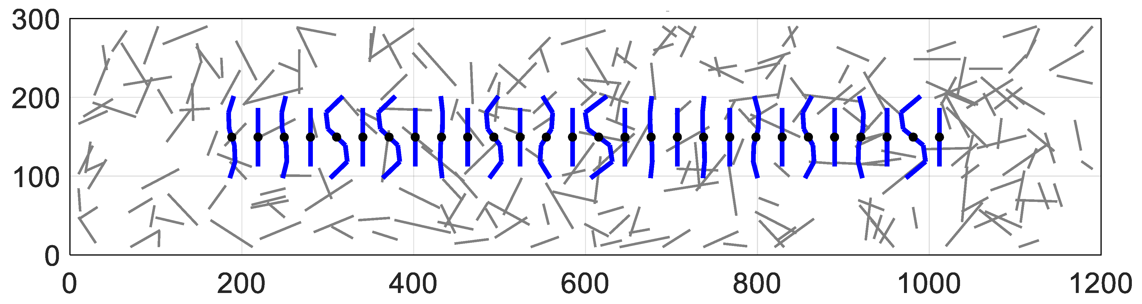
To illustrate the ShOpen capability of modular design and fast prototyping, a simulation of a reservoir having the geometry and properties of the Barnett shale reservoir, also including a 248-N-fractures stochastic DFN, is described (simulation AE2, see Figure 22). The DFN is generated by resorting to the open-source fracture generator ADFNE [61]. In addition, some of the H fractures are curvilinear. The indirect hydromechanical coupling is assumed (Equations (16)–(18)). The geomechanical parameters for shale reservoir are reported in Table 6. The remaining input data refers to Table 2 and Table 5.
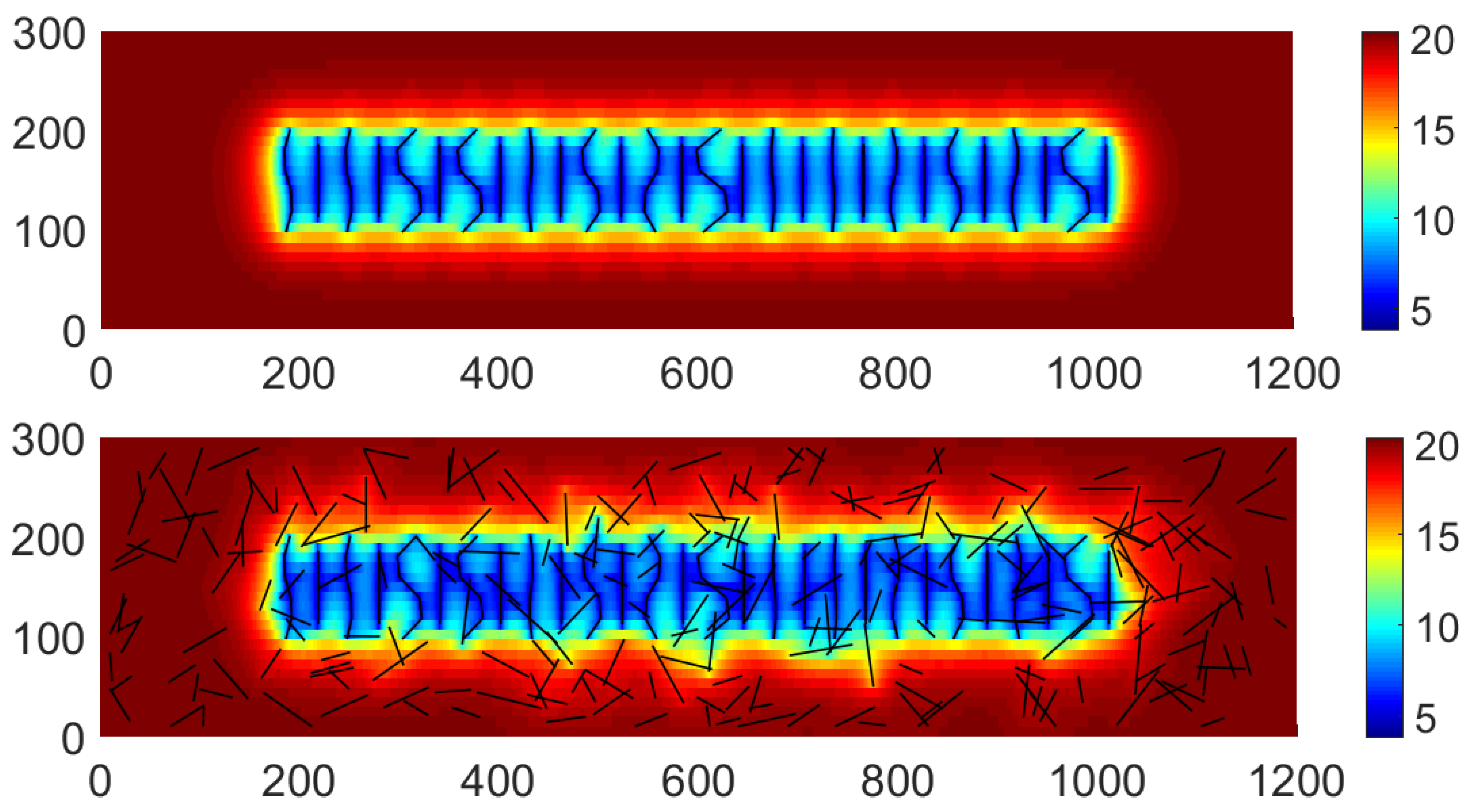
To evaluate the run-time performance of our code, the domain is discretized by using 5001 × 31 cells. For a computer with a Core I9-9820X CPU, the EDFM preprocessing time and computational time of this case required 405 s and 361 s, respectively. The results of a first simulation for a scenario with the H fractures are only compared to those for a scenario including the DFN. In Figure 23, the pressure contours after 3.75 years for the two scenarios are reported. As expected, with the inclusion of the DFN, a larger Stimulated Reservoir Volume (SRV) is experienced.
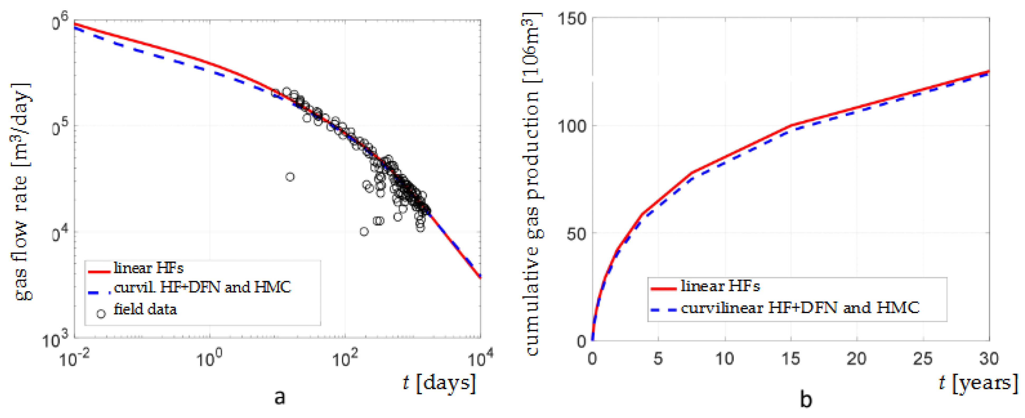
The effect of the HM coupling on well performance is investigated by implementing Equations (16)–(18). In Figure 24, a comparison is given between the results of a scenario with curvilinear HFs, DFN, and HM coupling and those of the scenario with linear HFs only. In the short term, the occurrence of HM coupling leads to a reduction in gas production; however, in the long term, the discrepancy between the two scenarios is negligible. Thus, the proper consideration of the HM coupling is relevant when dealing with the short-term performance.
6. Conclusions
In this work, a numerical code and an open-source framework ShOpen for simulations of unconventional gas reservoirs are described. The model encompasses up-to-date algorithms for fluid flow and transport mechanisms. Comparisons with the results provided by a commercial simulator and an in-house simulator are also reported for the validation of the code. Application examples are also illustrated. Some statements follow:
- the algorithms of the code refer to gas adsorption, gas slippage and diffusion, non-Darcy flow, and hydromechanical coupling;
- with the aid of EDFM, automatic differentiation, and a modular-designed framework, the use of ShOpen can be extended to shale gas reservoirs with embedded natural and/or artificial fractures of arbitrary fracture geometries and mutual connections;
- EDFM algorithms, implemented in ShOpen, can efficiently and accurately model stochastic DFNs, however, when dealing with low-permeability (natural) fractures and hydraulic fractures with strong gradients in the near-field, substantial errors are experienced, thus, the resort to LGR and an improved EDFM algorithm [30] are recommended;
- shale gas adsorption and transport mechanisms have a significant impact on well performance; less dramatic is the impact of HM coupling and the complexity of the DFN;
- ShOpen is an efficient and flexible tool for research investigations and practical applications for the implementation of nonlinearities and the fast handling of fracture networks.
Author Contributions
B.W.: conceptualization, code implementation, numerical analyses; C.F.: conceptualization (revision), editing. All authors have read and agreed to the published version of the manuscript.
Funding
This research received no external funding.
Acknowledgments
We would like to acknowledge discussions with Olufemi Olorode for the assistance in the implementation of EDFM. Source code and example cases are available at https://github.com/BinWang0213/MRST_Shale/tree/ShOpen (accessed on 23 February 2021).
Conflicts of Interest
The authors declare no conflict of interest.
References
- Bowker, K. Barnett Shale gas production, Fort Worth Basin: Issues and discussion. AAPG Bull. 2007, 91, 523–533. [Google Scholar] [CrossRef]
- Akkutlu, I.Y.; Efendiev, Y.; Vasilyeva, M.; Wang, Y. Multiscale model reduction for shale gas transport in poroelastic fractured media. J. Comput. Phys. 2018, 353, 356–376. [Google Scholar] [CrossRef]
- Gensterblum, Y.; Ghanizadeh, A.; Cuss, R.J.; Amann-Hildenbrand, A.; Krooss, B.M.; Clarkson, C.R.; Harrington, J.F.; Zoback, M.D. Gas transport and storage capacity in shale gas reservoirs—A review. Part A: Transport processes. J. Unconv. Oil Gas Resour. 2015, 12, 87–122. [Google Scholar] [CrossRef]
- Chen, L.; Jiang, Z.; Liu, K.; Gao, F. Quantitative characterization of micropore structure for organic-rich Lower Silurian shale in the Upper Yangtze Platform, South China: Implications for shale gas adsorption capacity. Adv. Geo-Energy Res. 2017, 1, 112–123. [Google Scholar] [CrossRef] [Green Version]
- Gringarten, A.C.; Ramey, H.J.; Raghavan, R. Unsteady-state pressure distributions created by a well with a single infinite-conductivity vertical fracture. Soc. Pet. Eng. J. 1974, 14, 347–360. [Google Scholar] [CrossRef] [Green Version]
- Cinco Ley, H.; Samaniego, F.; Dominguez, A.N. Transient pressure behavior for a well with a finite-conductivity vertical fracture. Soc. Pet. Eng. J. 1976, 18, 253–264. [Google Scholar] [CrossRef] [Green Version]
- Zuo, L.; Yu, W.; Wu, K. A fractional decline curve analysis model for shale gas reservoirs. Int. J. Coal Geol. 2016, 163, 140–148. [Google Scholar] [CrossRef]
- Yu, W.; Wu, K.; Sepehrnoori, K.; Xu, W. A comprehensive model for simulation of gas transport in shale formation with complex hydraulic-fracture geometry. Soc. Pet. Eng. J. 2017, 20. [Google Scholar] [CrossRef]
- Chen, Z.; Liao, X.; Sepehrnoori, K.; Yu, W. A semianalytical model for pressure-transient analysis of fractured wells in unconventional plays with arbitrarily distributed discrete fractures. Soc. Pet. Eng. J. 2018, 23. [Google Scholar] [CrossRef]
- Li, Y.; Zuo, L.; Yu, W.; Chen, Y. A fully three dimensional semi-analytical model for shale gas reservoirs with hydraulic fractures. Energies 2018, 11, 436. [Google Scholar] [CrossRef] [Green Version]
- Wang, B.; Feng, Y.; Du, J.; Wang, Y.; Wang, S.; Yang, R. An embedded grid-free approach for near-wellbore streamline simulation. SPE J. 2018, 23, 567–588. [Google Scholar] [CrossRef]
- Wang, B.; Feng, Y.; Pieraccini, S.; Scialò, S.; Fidelibus, C. Iterative coupling algorithms for large multidomain problems with the boundary element method. Int. J. Numer. Methods Eng. 2019, 117, 1–14. [Google Scholar] [CrossRef] [Green Version]
- Chen, Z.; Liao, X.; Zhao, X.; Dou, X.; Zhu, L. Performance of horizontal wells with fracture networks in shale gas formation. J. Pet. Sci. Eng. 2015, 133, 646–664. [Google Scholar] [CrossRef]
- Chen, Z.; Liao, X.; Zhao, X.; Lv, S.; Zhu, L. A semianalytical approach for obtaining type curves of multiple-fractured horizontal wells with secondary-fracture networks. SPE J. 2016, 21, 538–549. [Google Scholar] [CrossRef]
- Olorode, O.M.; Akkutlu, I.Y.; Efendiev, Y. Compositional reservoir-flow simulation for organic-rich gas shale. Soc. Pet. Eng. J. 2017, 22. [Google Scholar] [CrossRef]
- Cipolla, C.; Lolon, E.; Erdle, J.; Rubin, B. Reservoir modeling in shale-gas reservoirs. SPE Reserv. Eval. Eng. 2013, 13, 638–653. [Google Scholar] [CrossRef]
- de Dreuzy, J.R.; Davy, P.; Bour, O. Hydraulic properties of two-dimensional random fracture networks following power-law distributions of length and aperture. Water Resour. Res. 2002, 38, 12-1–12-9. [Google Scholar] [CrossRef]
- Lee, S.H.; Lough, M.F.; Jensen, C.L. Hierarchical modeling of flow in naturally fractured formations with multiple length scales. Water Resour. Res. 2001, 37, 443–455. [Google Scholar] [CrossRef]
- Karimi-Fard, M.; Gong, B.; Durlofsky, L.J. Generation of coarse-scale continuum flow models from detailed fracture characterizations. Water Resour. Res. 2006, 42. [Google Scholar] [CrossRef]
- Karimi-Fard, M.; Durlofsky, L. A general gridding, discretization, and coarsening methodology for modeling flow in porous formations with discrete geological features. Adv. Water Resour. 2016, 96, 354–372. [Google Scholar] [CrossRef]
- Miao, J.; Yu, W.; Xia, Z.; Zhao, W.; Xu, Y.; Sepehrnoori, K. An Easy and Fast EDFM Method for Production Simulation in Shale Reservoirs with Complex Fracture Geometry. In Proceedings of the 2nd International Discrete Fracture Network Engineering Conference, Seattle, WA, USA, 20–22 June 2018; American Rock Mechanics Association: Richardson, TX, USA, 2018. [Google Scholar]
- Xu, J.; Chen, B.; Sun, B.; Jiang, R. Flow behavior of hydraulic fractured tight formations considering Pre-Darcy flow using EDFM. Fuel 2019, 241, 1145–1163. [Google Scholar] [CrossRef]
- Xue, X.; Yang, C.; Onishi, T.; King, M.J.; Datta-Gupta, A. Modeling Hydraulically Fractured Shale Wells Using the Fast-Marching Method With Local Grid Refinements and an Embedded Discrete Fracture Model. SPE J. 2019, 24, 2590–2608. [Google Scholar] [CrossRef]
- Wan, X.; Rasouli, V.; Damjanac, B.; Yu, W.; Xie, H.; Li, N.; Rabiei, M.; Miao, J.; Liu, M. Coupling of fracture model with reservoir simulation to simulate shale gas production with complex fractures and nanopores. J. Pet. Sci. Eng. 2020, 193, 107422. [Google Scholar] [CrossRef]
- Bai, Y.; Liu, L.; Fan, W.; Sun, H.; Huang, Z.; Yao, J. Coupled compositional flow and geomechanics modeling of fractured shale oil reservoir with confined phase behavior. J. Pet. Sci. Eng. 2021, 196, 107608. [Google Scholar] [CrossRef]
- Cai, J.; Lin, D.; Singh, H.; Wei, W.; Zhou, S. Shale gas transport model in 3D fractal porous media with variable pore sizes. Mar. Pet. Geol. 2018, 98, 437–447. [Google Scholar] [CrossRef]
- Cai, J.; Lin, D.; Singh, H.; Zhou, S.; Meng, Q.; Zhang, Q. A simple permeability model for shale gas and key insights on relative importance of various transport mechanisms. Fuel 2019, 252, 210–219. [Google Scholar] [CrossRef]
- Zhang, T.; Sun, S.; Song, H. Flow mechanism and simulation approaches for shale gas reservoirs: A review. Transp. Porous Media 2019, 126, 655–681. [Google Scholar] [CrossRef] [Green Version]
- Ning, X.; Feng, Y.; Wang, B. Numerical simulation of channel fracturing technology in developing shale gas reservoirs. J. Nat. Gas Sci. Eng. 2020, 83, 103515. [Google Scholar] [CrossRef]
- Ţene, M.; Bosma, S.B.; Al Kobaisi, M.S.; Hajibeygi, H. Projection-based Embedded Discrete Fracture Model (pEDFM). Adv. Water Resour. 2017, 105, 205–216. [Google Scholar] [CrossRef]
- Yang, R.; Huang, Z.; Yu, W.; Li, G.; Ren, W.; Zuo, L.; Tan, X.; Sepehrnoori, K.; Tian, S.; Sheng, M. A comprehensive model for real gas transport in shale formations with complex non-planar fracture networks. Sci. Rep. 2016, 6, 36673. [Google Scholar] [CrossRef] [Green Version]
- Peng, D.Y.; Robinson, D.B. A new two-constant equation of state. Ind. Eng. Chem. Fundam. 1976, 15, 59–64. [Google Scholar] [CrossRef]
- Elliott, J.R.; Lira, C.T. Introductory Chemical Engineering Thermodynamics; Prentice-Hall International Series in the Physical and Chemical Engineering Sciences; Prentice Hall: Upper Saddle River, NJ, USA, 2012. [Google Scholar]
- Mahmoud, M. Development of a new correlation of gas compressibility factor (Z-factor) for high pressure gas reservoir. J. Energy Resour. Technol. 2013, 136, 012903. [Google Scholar] [CrossRef]
- Lee, A.L.; Gonzalez, M.H.; Eakin, B.E. The viscosity of natural gases. J. Pet. Technol. 1966, 18, 997–1000. [Google Scholar] [CrossRef]
- Klinkenberg, L.J. The permeability of porous media to liquids and gases. In Drilling and Production Practice; American Petroleum Institute: New York, NY, USA, 1941. [Google Scholar]
- Florence, F.A.; Rushing, J.; Newsham, K.E.; Blasingame, T.A. Improved permeability prediction relations for low permeability sands. In Proceedings of the SPE Rocky Mountain Oil & Gas Technology Symposium, Denver, CO, USA, 16–18 April 2007; Society of Petroleum Engineers: Tyler, TX, USA, 2007. [Google Scholar]
- Javadpour, F.; Fisher, D.; Unsworth, M. Nanoscale gas flow in shale gas sediments. J. Can. Pet. Technol. 2007, 46. [Google Scholar] [CrossRef]
- Civan, F. Effective correlation of apparent gas permeability in tight porous media. Transp. Porous Media 2010, 82, 375–384. [Google Scholar] [CrossRef]
- Yu, W.; Sepehrnoori, K.; Patzek, T.W. Modeling gas adsorption in Marcellus shale with Langmuir and BET isotherms. Soc. Pet. Eng. J. 2016, 21, 589–600. [Google Scholar] [CrossRef] [Green Version]
- Shen, W.; Li, X.; Cihan, A.; Lu, X.; Liu, X. Experimental and numerical simulation of water adsorption and diffusion in shale gas reservoir rocks. Adv. Geo-Energy Res. 2019, 3, 165–174. [Google Scholar] [CrossRef]
- Zeng, Z.; Grigg, R. A criterion for non-Darcy flow in porous media. Transp. Porous Media 2006, 63, 57–69. [Google Scholar] [CrossRef]
- Barree, R.D.; Conway, M.W. Beyond beta factors: A complete model for Darcy, Forchheimer, and trans-Forchheimer flow in porous media. In Proceedings of the SPE Annual Technical Conference and Exhibition, Houston, TX, USA, 26–29 September 2004; Society of Petroleum Engineers: Tyler, TX, USA, 2004. [Google Scholar]
- Rubin, B. Accurate simulation of non-Darcy flow in stimulated fractured shale reservoirs. In Proceedings of the SPE Western Regional Meeting, Anaheim, CA, USA, 27–29 May 2010; Society of Petroleum Engineers: Tyler, TX, USA, 2010. [Google Scholar]
- Hu, X.; Wu, K.; Li, G.; Tang, J.; Shen, Z. Effect of proppant addition schedule on the proppant distribution in a straight fracture for slickwater treatment. J. Pet. Sci. Eng. 2018, 167, 110–119. [Google Scholar] [CrossRef]
- Wang, H.F. Theory of Linear Poroelasticity; Princeton University Press: Princeton, NJ, USA, 2000. [Google Scholar]
- Rutqvist, J.; Stephansson, O. The role of hydromechanical coupling in fractured rock engineering. Hydrogeol. J. 2003, 11, 7–40. [Google Scholar] [CrossRef] [Green Version]
- Cammarata, G.; Fidelibus, C.; Cravero, M.; Barla, G. The hydro-mechanically coupled response of rock fractures. Rock Mech. Rock Eng. 2007, 40, 41–61. [Google Scholar] [CrossRef]
- Fidelibus, C. The 2D hydro-mechanically coupled response of a rock mass with fractures via a mixed BEM–FEM technique. Int. J. Numer. Anal. Methods Geomech. 2007, 31, 1329–1348. [Google Scholar] [CrossRef]
- Hu, M.; Wang, Y.; Rutqvist, J. Fully coupled hydro-mechanical numerical manifold modeling of porous rock with dominant fractures. Acta Geotech. 2017, 12, 231–252. [Google Scholar] [CrossRef] [Green Version]
- Gangi, A.F. Variation of whole and fractured porous rock permeability with confining pressure. Int. J. Rock Mech. Min. Sci. Geomech. Abstr. 1978, 15, 249–257. [Google Scholar] [CrossRef]
- Shi, J.Q.; Durucan, S. Near-exponential relationship between effective stress and permeability of porous rocks revealed in Gangi’s phenomenological models and application to gas shales. Int. J. Coal Geol. 2016, 154, 111–122. [Google Scholar] [CrossRef] [Green Version]
- Alramahi, B.; Sundberg, M.I. Proppant embedment and conductivity of hydraulic fractures in shales. In Proceedings of the 46th ARMA US Rock Mechanics/Geomechanics Symposium, Chicago, IL, USA, 24–27 June 2012; Society of Petroleum Engineers: Tyler, TX, USA, 2012. [Google Scholar]
- Wu, W.; Zhou, J.; Kakkar, P.; Russell, R.; Sharma, M.M. An experimental study on conductivity of unpropped fractures in preserved shales. Soc. Pet. Eng. J. 2019, 34, 280–296. [Google Scholar] [CrossRef]
- Lie, K.; Krogstad, S.; Ligaarden, I.S.; Natvig, J.R.; Nilsen, H.M.; Skaflestad, B. Open-source MATLAB implementation of consistent discretisations on complex grids. Comput. Geosci. 2012, 16, 297–322. [Google Scholar] [CrossRef] [Green Version]
- Xu, Y. Implementation and application of the Embedded Discrete Fracture Model (EDFM) for Reservoir Simulation in Fractured Reservoirs. Master’s Thesis, The University of Texas at Austin, Austin, TX, USA, 2015. [Google Scholar]
- Ţene, M.; Al Kobaisi, M.S.; Hajibeygi, H. Algebraic multiscale method for flow in heterogeneous porous media with embedded discrete fractures (F-AMS). J. Comput. Phys. 2016, 321, 819–845. [Google Scholar] [CrossRef] [Green Version]
- Karimi-Fard, M.; Durlofsky, L.J.; Aziz, K. An efficient discrete fracture model applicable for general purpose reservoir simulators. In Proceedings of the SPE Reservoir Simulation Symposium, Houston, TX, USA, 3–5 February 2003; Society of Petroleum Engineers: Tyler, TX, USA, 2003. [Google Scholar]
- Jiang, J.; Younis, R.M. Numerical study of complex fracture geometries for unconventional gas reservoirs using a discrete fracture-matrix model. J. Nat. Gas Sci. Eng. 2015, 26, 1174–1186. [Google Scholar] [CrossRef]
- Cao, P.; Liu, J.; Leong, Y.K. A fully coupled multiscale shale deformation-gas transport model for the evaluation of shale gas extraction. Fuel 2016, 178, 103–117. [Google Scholar] [CrossRef]
- Fadakar Alghalandis, Y. ADFNE: Open source software for discrete fracture network engineering, two and three dimensional applications. Comput. Geosci. 2017, 102, 1–11. [Google Scholar] [CrossRef]
Figure 1.
Shale gas production: (a) gas transport, (b) multiscale features.

Figure 2.
Natural gas Z-factor for methane estimated by Peng–Robinson Equation-Of-State (PR-EOS) [32] and empirical equation [34]; T = 352 K, = 191 K, = 4.64 MPa, R = 8.314 JKmol.

Figure 3.
Methane viscosity (in cp, 1 cp = 1 mPa·s) estimated by the Lee–Gonzalez–Eakin empirical correlation [35] with M = 16.04 g/mol and T = 633.6 R.
Figure 3.
Methane viscosity (in cp, 1 cp = 1 mPa·s) estimated by the Lee–Gonzalez–Eakin empirical correlation [35] with M = 16.04 g/mol and T = 633.6 R.

Figure 4.
Langmuir and BET isotherms for = 0.0031 m/kg, = 7.89 MPa, T = 327.59 K, = 53.45 MPa, = 0.0015 m/kg, C = 24.56, and n = 4.46.
Figure 4.
Langmuir and BET isotherms for = 0.0031 m/kg, = 7.89 MPa, T = 327.59 K, = 53.45 MPa, = 0.0015 m/kg, C = 24.56, and n = 4.46.

Figure 5.
Permeability correction factor plotted against the Knudesen number for methane (T = 191 K, = m, = 0.1) with flow fields.
Figure 5.
Permeability correction factor plotted against the Knudesen number for methane (T = 191 K, = m, = 0.1) with flow fields.

Figure 6.
Permeability correction factor versus gas pressure with m = 0.5, = 0.5, = 180 MPa, = 38 MPa, and = 0.5.
Figure 6.
Permeability correction factor versus gas pressure with m = 0.5, = 0.5, = 180 MPa, = 38 MPa, and = 0.5.

Figure 7.
Normalized fracture conductivity plotted against the effective normal stress on a fracture for (a) propped fractures and (b) unpropped fractures.
Figure 7.
Normalized fracture conductivity plotted against the effective normal stress on a fracture for (a) propped fractures and (b) unpropped fractures.

Figure 8.
Permeability correction factor for hydraulic fractures and natural fractures with pressure = 34.5 MPa, = 29 MPa, and = 34 MPa.
Figure 8.
Permeability correction factor for hydraulic fractures and natural fractures with pressure = 34.5 MPa, = 29 MPa, and = 34 MPa.

Figure 9.
Nodes in an EDFM for the matrix, a hydraulic fracture, and a natural fracture.

Figure 10.
Scheme for the comparison with the CMG (Computer Modelling Group Ltd.) simulator (simulations VE1A, VE1B).
Figure 10.
Scheme for the comparison with the CMG (Computer Modelling Group Ltd.) simulator (simulations VE1A, VE1B).

Figure 11.
Results of the VE1A simulation: (a) gas flow rate and (b) cumulative gas production versus time t for fracture conductivity equal to 5 (green lines), 50 (blue lines) and 10,000 (red lines) mD-ft. Solid lines—ShOpen/EDFM; dashed lines—ShOpen/EFM; circles—CMG.
Figure 11.
Results of the VE1A simulation: (a) gas flow rate and (b) cumulative gas production versus time t for fracture conductivity equal to 5 (green lines), 50 (blue lines) and 10,000 (red lines) mD-ft. Solid lines—ShOpen/EDFM; dashed lines—ShOpen/EFM; circles—CMG.

Figure 12.
Grids for VE1B sensitivity analysis simulations: (a) Local Grid Refinement (LGR), (b) EDFM, (c) LGR+EDFM; the fracture cell is magnified 10 times.
Figure 12.
Grids for VE1B sensitivity analysis simulations: (a) Local Grid Refinement (LGR), (b) EDFM, (c) LGR+EDFM; the fracture cell is magnified 10 times.

Figure 13.
Comparison of the results provided by ShOpen and CMG in terms of (a) gas flow rate and (b) cumulative production, for VE1B with 10,000 mD-ft.
Figure 13.
Comparison of the results provided by ShOpen and CMG in terms of (a) gas flow rate and (b) cumulative production, for VE1B with 10,000 mD-ft.

Figure 14.
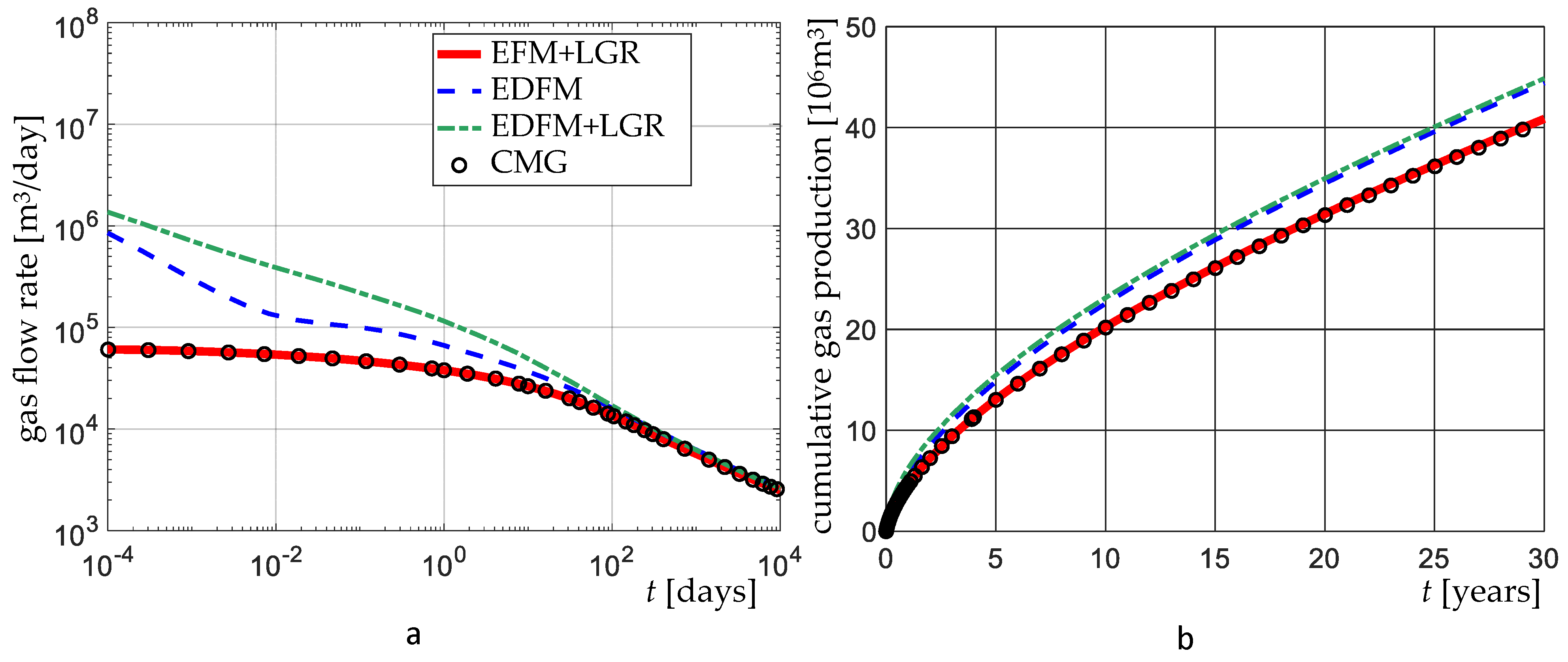
Comparison of the results provided by ShOpen and CMG in terms of (a) gas flow rate and (b) cumulative production, for VE1B with 5 mD-ft.
Figure 14.
Comparison of the results provided by ShOpen and CMG in terms of (a) gas flow rate and (b) cumulative production, for VE1B with 5 mD-ft.

Figure 15.
Grids for VE1C simulation: (a) LGR, (b) EDFM, (c) LGR+EDFM.

Figure 16.
Comparison of the results provided by using the different grids in terms of (a) gas flow rate and (b) normalized cumulative gas production, for VE1C.
Figure 16.
Comparison of the results provided by using the different grids in terms of (a) gas flow rate and (b) normalized cumulative gas production, for VE1C.

Figure 17.
Scheme for the comparison with the in-house simulator (simulation VE2).

Figure 18.
Gas flow rate (a) of VE2 and cumulative gas production (b) for adsorption and slippage/diffusion, adsorption only, slippage/diffusion only, and no mechanisms; comparison between ShOpen and the in-house simulator [59].
Figure 18.
Gas flow rate (a) of VE2 and cumulative gas production (b) for adsorption and slippage/diffusion, adsorption only, slippage/diffusion only, and no mechanisms; comparison between ShOpen and the in-house simulator [59].

Figure 19.
AE1 simulation scheme (top) and relative EDFM grid with 28 linear HFs (bottom).

Figure 20.
Pressure contours after 1600 days for the Barnett shale reservoir (simulation AE1).

Figure 21.
History matching (a) and prediction (b) of the gas production rate in the Barnett shale reservoir (simulation AE1).
Figure 21.
History matching (a) and prediction (b) of the gas production rate in the Barnett shale reservoir (simulation AE1).

Figure 22.
Scheme of simulation AE2 showing the 28 HFs and the 248 NFs.

Figure 23.
Pressure contours at 3.75 years for the Barnett shale reservoir (simulation AE2) for the scenario with curvilinear HFs (top) and for the scenario with the DFN added (bottom).
Figure 23.
Pressure contours at 3.75 years for the Barnett shale reservoir (simulation AE2) for the scenario with curvilinear HFs (top) and for the scenario with the DFN added (bottom).

Figure 24.
Comparison of gas flow rate (a) and cumulative production (b) between the scenario with linear HFs and the scenario with curvilinear HFs and DFN and, in addition, consideration of HMC (simulation AE2).
Figure 24.
Comparison of gas flow rate (a) and cumulative production (b) between the scenario with linear HFs and the scenario with curvilinear HFs and DFN and, in addition, consideration of HMC (simulation AE2).


Table 1.
Comparison of methods for the prediction of gas transport in unconventional reservoirs; : nonlinear gas transport and storage, multiphase and multicomponent flow. DFN—Discrete Fracture Networks, EDFM—Embedded Discrete Fracture Model.
Table 1.
Comparison of methods for the prediction of gas transport in unconventional reservoirs; : nonlinear gas transport and storage, multiphase and multicomponent flow. DFN—Discrete Fracture Networks, EDFM—Embedded Discrete Fracture Model.
| Analytical | Semianalytical | Structured Grid | Unstructured Grid | EDFM | |
|---|---|---|---|---|---|
| accuracy | ++ | ++ | +++ | +++ | ++ |
| handling nonlinear mechanisms | + | + | +++ | +++ | +++ |
| handling rock heterogeneity | + | + | +++ | +++ | +++ |
| quality of DFN mesh | +++ | +++ | + | + | +++ |
| preprocessing efficiency | +++ | +++ | +++ | +++ | ++ |
| computational efficiency | +++ | +++ | + | ++ | ++ |
Table 2.
Adsorption and transport, corresponding models and domain for the gas flow; A—adsorption, T—transport.
Table 2.
Adsorption and transport, corresponding models and domain for the gas flow; A—adsorption, T—transport.
| Mechanism | Model | Type | Domain |
|---|---|---|---|
| adsorption | Langmuir, BET | A | matrix |
| slip flow/diffusion | Klinkenberg [36], Florence et al. [37], Javadpour et al. [38], Civan [39] | T | matrix |
| non-Darcy flow | Darcy–Forchheimer | T | fracture |
Table 3.
Input data of the simulations for the comparison with CMG. BHP—bottom-hole pressure.
| Property | Unit | Value |
|---|---|---|
| domain dimensions | m | 606.6 × 606.6 |
| formation thickness | m | 45.72 |
| initial reservoir pressure | MPa | 34.47 |
| reservoir temperature T | K | 327.60 |
| Langmuir pressure | MPa | 8.96 |
| Langmuir volume | m/kg | 0.0041 |
| matrix porosity | - | 0.07 |
| matrix compressibility | 1/Pa | 1.45 × 10 |
| matrix permeability | nD | 500 |
| fracture permeability | mD | 0.5–1000 |
| fracture width w | m | 0.003 |
| fracture half-length ½ | m | 106.68 |
| fracture conductivity | mD-ft | 5–10,000 |
| well BHP | MPa | 3.45 |
Table 4.
Key reservoir and simulation parameters of VE2.
| Property | Unit | Value |
|---|---|---|
| domain dimensions | m | 200,140 |
| formation thickness | m | 10 |
| initial reservoir pressure | MPa | 16 |
| reservoir temperature T | K | 343.15 |
| Langmuir pressure | MPa | 4 |
| Langmuir volume | m/kg | 0.018 |
| matrix porosity | - | 0.1 |
| matrix compressibility | 1/Pa | 1.0 × |
| matrix permeability | nD | 100 |
| fracture porosity | - | 1.0 |
| fracture permeability | D | 1 |
| fracture width w | m | 1× |
| well BHP | MPa | 4 |
| wellbore skin factor s | - | 43 |
| Property | Unit | Value |
|---|---|---|
| domain dimensions | m | 1200,300 |
| formation thickness | m | 90 |
| initial reservoir pressure | MPa | 20.34 |
| reservoir temperature T | K | 352 |
| rock density | kg/m | 2500 |
| Langmuir pressure | MPa | 4.47 |
| Langmuir volume | m/kg | 0.00272 |
| matrix porosity | - | 0.1 |
| matrix compressibility | 1/Pa | 1.0 × |
| matrix permeability | nD | 200 |
| fracture porosity | - | 0.03 |
| fracture permeability | D | 1.0 × |
| fracture width w | m | 0.003 |
| fracture half-length ½ | m | 47.2 |
| fracture conductivity | mD-ft | 1 |
| well bottom-hole pressure BHP | MPa | 3.69 |
| wellbore skin factor s | - | 19 |
Table 6.
Geomechanical parameters of Barnett shale for simulation AE2; the other input data are shown in Table 2 and Table 5.
| Property | Unit | Value |
|---|---|---|
| Biot coefficient | - | 0.5 |
| overburden stress | MPa | 38 |
| maximum horizontal stress | MPa | 34 |
| minimum horizontal stress | MPa | 29 |
| effective modulus of the asperities | MPa | 180 |
| Gangi exponential constant m | - | 0.5 |
| N fracture permeability | mD | 10 |
Publisher’s Note: MDPI stays neutral with regard to jurisdictional claims in published maps and institutional affiliations. |
© 2021 by the authors. Licensee MDPI, Basel, Switzerland. This article is an open access article distributed under the terms and conditions of the Creative Commons Attribution (CC BY) license (http://creativecommons.org/licenses/by/4.0/).
Share and Cite
MDPI and ACS Style
Wang, B.; Fidelibus, C. An Open-Source Code for Fluid Flow Simulations in Unconventional Fractured Reservoirs. Geosciences 2021, 11, 106. https://0-doi-org.brum.beds.ac.uk/10.3390/geosciences11020106
AMA Style
Wang B, Fidelibus C. An Open-Source Code for Fluid Flow Simulations in Unconventional Fractured Reservoirs. Geosciences. 2021; 11(2):106. https://0-doi-org.brum.beds.ac.uk/10.3390/geosciences11020106
Chicago/Turabian StyleWang, Bin, and Corrado Fidelibus. 2021. "An Open-Source Code for Fluid Flow Simulations in Unconventional Fractured Reservoirs" Geosciences 11, no. 2: 106. https://0-doi-org.brum.beds.ac.uk/10.3390/geosciences11020106
Note that from the first issue of 2016, this journal uses article numbers instead of page numbers. See further details here.