
3D Probabilistic Modelling and Uncertainty Analysis of Glacial and Post-Glacial Deposits of the City of Saguenay, Canada


Abstract
:1. Introduction
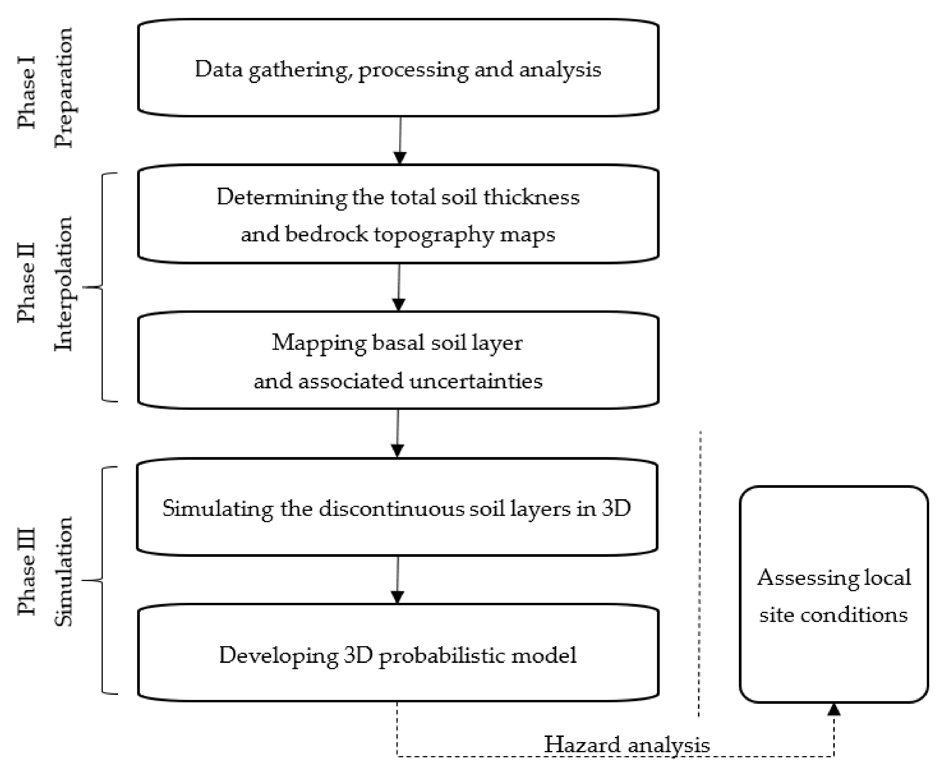
2. Methodology
3. Applied Geostatistical Methods
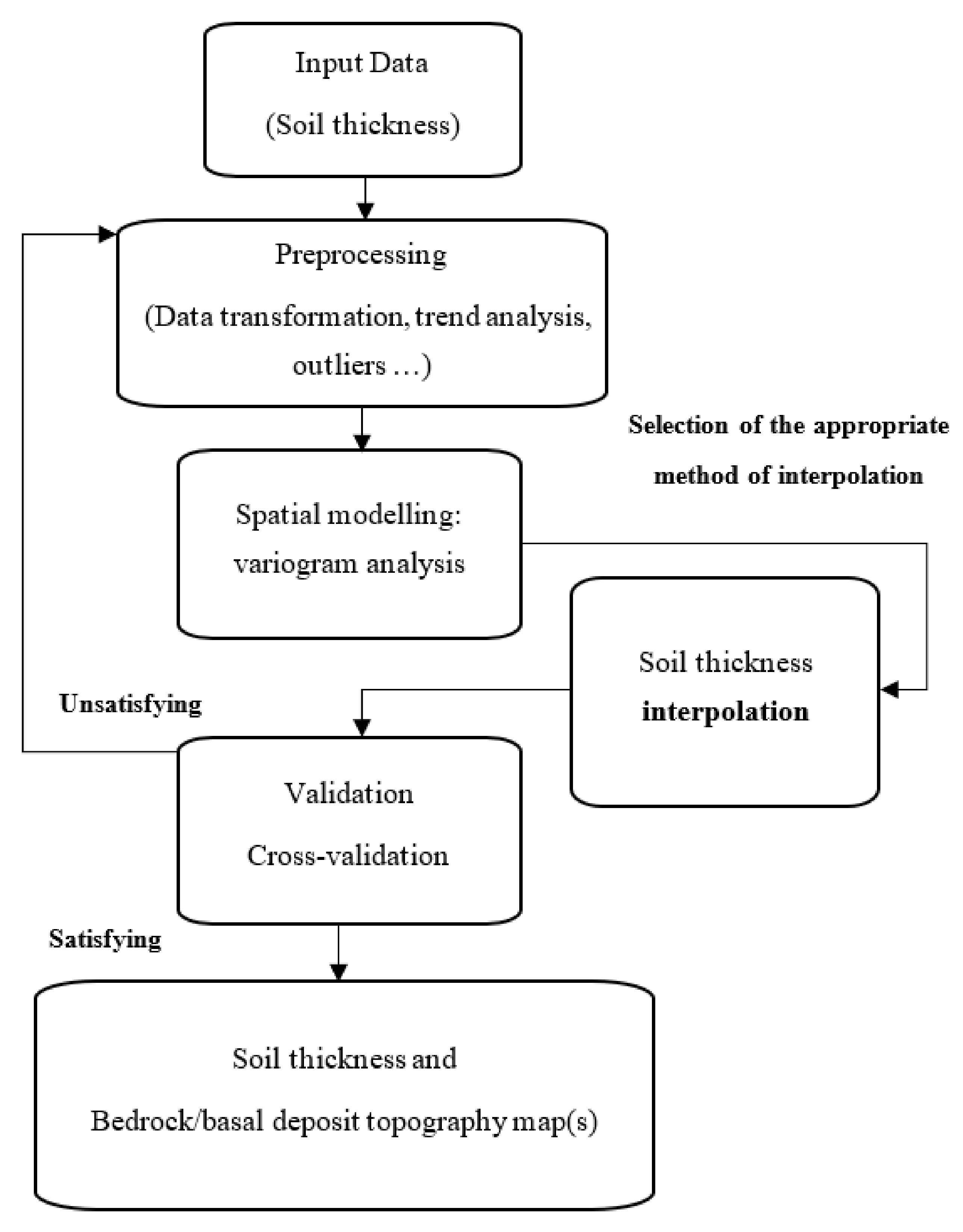
3.1. Spatial Interpolation
3.2. Spatial Variation
3.3. Uncertainty of Spatial Interpolation
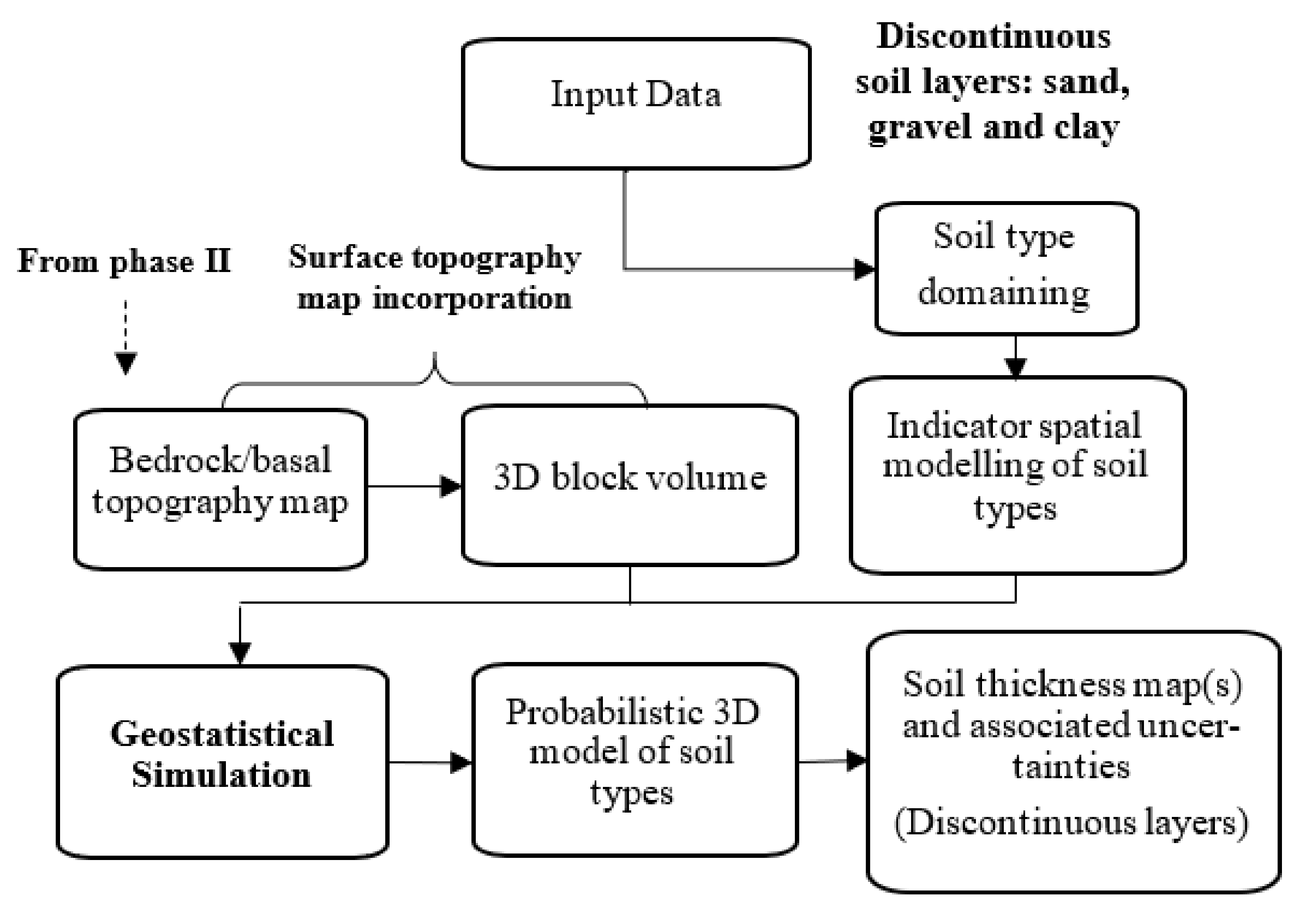
3.4. Stochastic Simulation
- (i)
- Transformation of soil types to K indicator variablesIndicator transformation facilitates classical statistical analyses to infer representative proportions of the indicator variables;
- (ii)
- Determination of indicator variograms to model the spatial continuity of the indicator soil types;
- (iii)
- Simulation of the soil types honouring field observation at sampled locations (conditional simulation) in a sequential and reproducible manner.
4. Saguenay City DatPreparation and Analysis
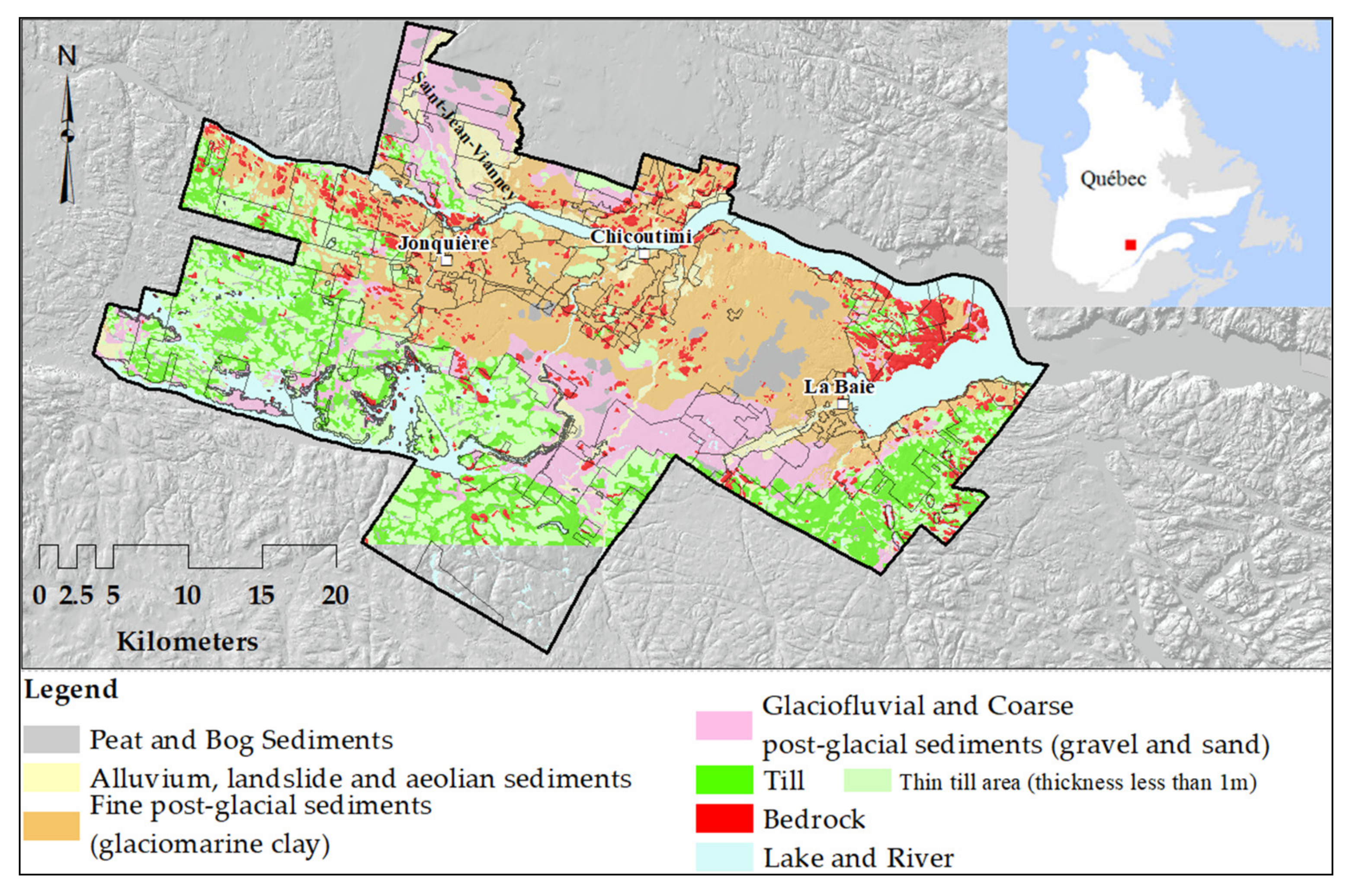
4.1. Geologic Framework of the Study Area
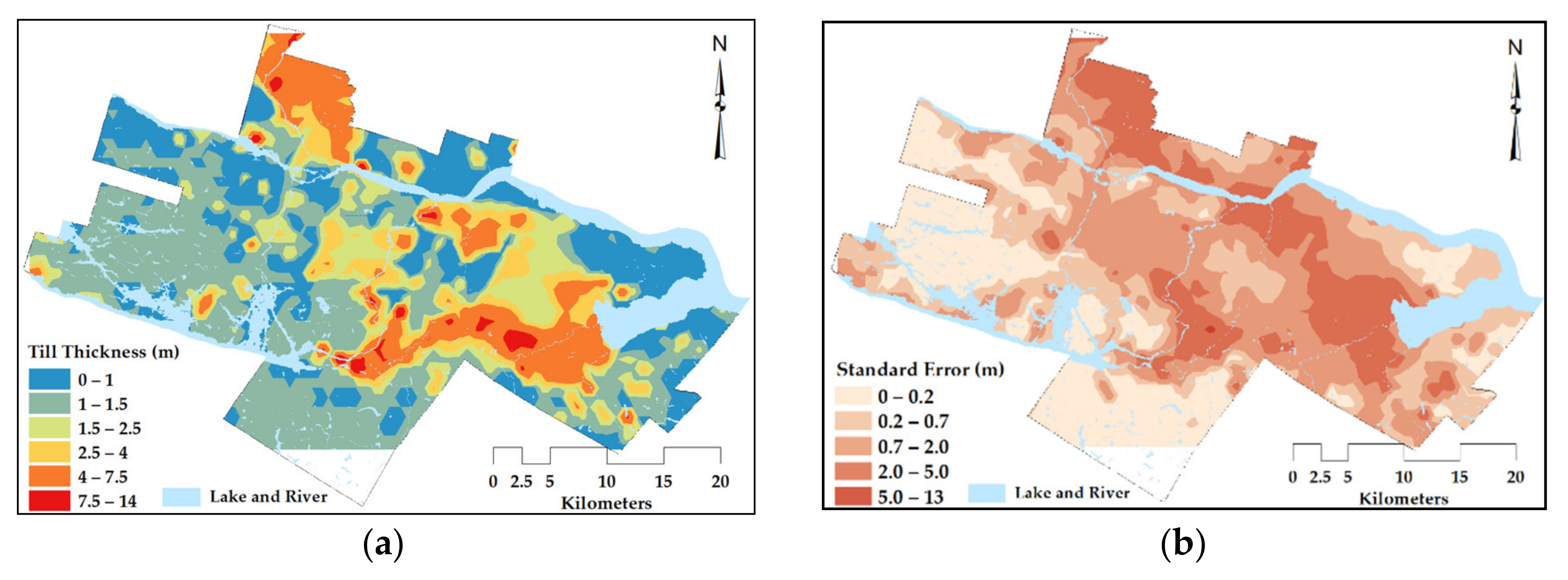
- Till: This glacial sediment is located at the base of the stratigraphic soil column; it is compact and semiconsolidated. Till is the most widespread soil unit in the study area and ranges in thickness from a few meters to >10 m at certain locations. In the highlands, the till veneer is frequently discontinuous and results in areas of rock outcrops. Most of the till outcrops are assumed to be less than 1 m thick on the geological map [33]. With the exception of rock outcrops, till continuously covers the bedrock elsewhere, representing an important assumption in the 3D modelling approach.
- Gravel: This coarse sediment is mainly of glaciofluvial and alluvial origin; it consists of gravel, sand and sometimes till. This unit is occasional in the region, often in contact with till or sand units.
- Clays: These fine post-glacial sediments are the most present soil type by volume in the study area. They are composed mainly of silt, silty clays and clay. They have a thickness of up to 10 m and may attain a maximum thickness of >100 m in the lowlands.
- Sand: This group consists mainly of coarse glaciomarine deltaic and prodeltaic sediments and alluvial sands composed of sand and gravely sands.
- Other sediments: This extremely heterogeneous category comprises all the remaining sediments; it mainly includes loose post-glacial sediments consisting of alluvium, floodplain sediments, organic sediments and occasional landslide colluvium that can be classified into sand, clay and gravel on the basis of grain size distribution.

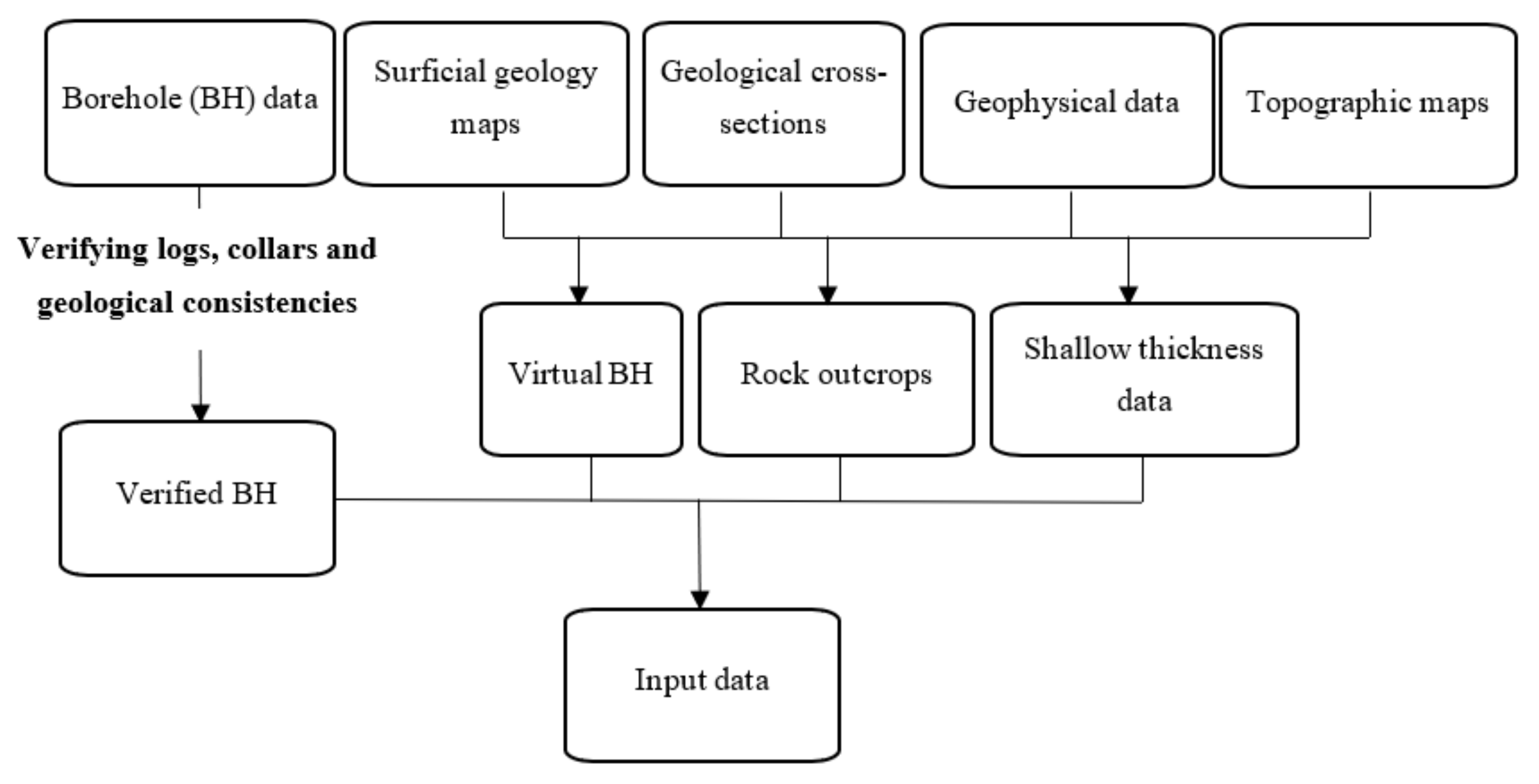
4.2. Input Data and Analysis
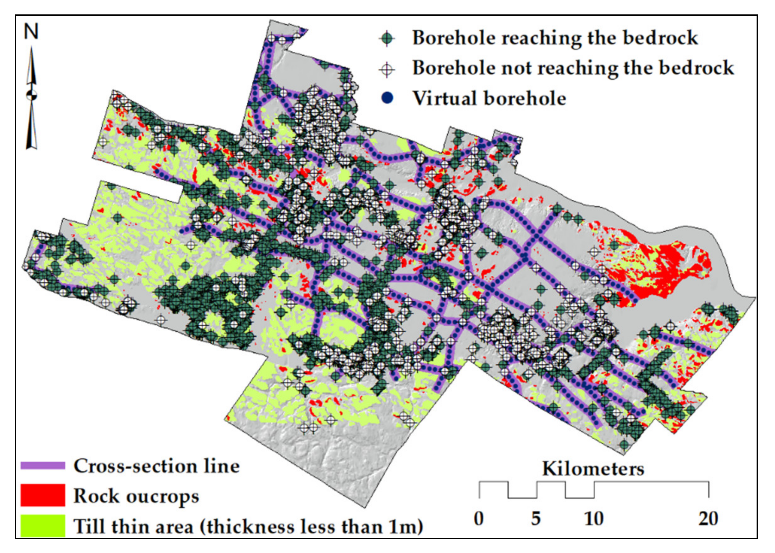
- Borehole logs: The database contains 3524 borehole logs distributed over the study area [34]. A total of 2402 boreholes are sufficiently deep to reach the bedrock. The remaining 1122 boreholes that do not reach the bedrock indicate that the bedrock is deeper than the borehole depth, and a groundwater-bearing layer is possibly encountered in the coarse soil deposits.
- Virtual logs: A total of 26 geological cross-sections distributed over the region were developed on the basis of expert opinion in previous geological studies [34]. These cross-sections include 973 virtual logs distributed in a regular spatial pattern at a distance of ~500 m to improve the data coverage mainly in the lowland areas (Figure 6).
- Rock outcrops: During the geographic information system processing of the surficial geology map, additional 1033 data points were introduced to indicate rock outcrops. Located within the bedrock polygons, they improve the realistic spatial variability of the sediment thickness.
- Till veneer: Till sediments cover most of the study area. Till outcropping areas, with a thickness equal to or less than 1.0 m, are located in the highlands and are referred to as a till veneer. In these areas, the till thickness is fixed to 1 m, and the till outcrop polygons are modelled with a mesh of 75 m, generating an additional 42,649 points with a known thickness.

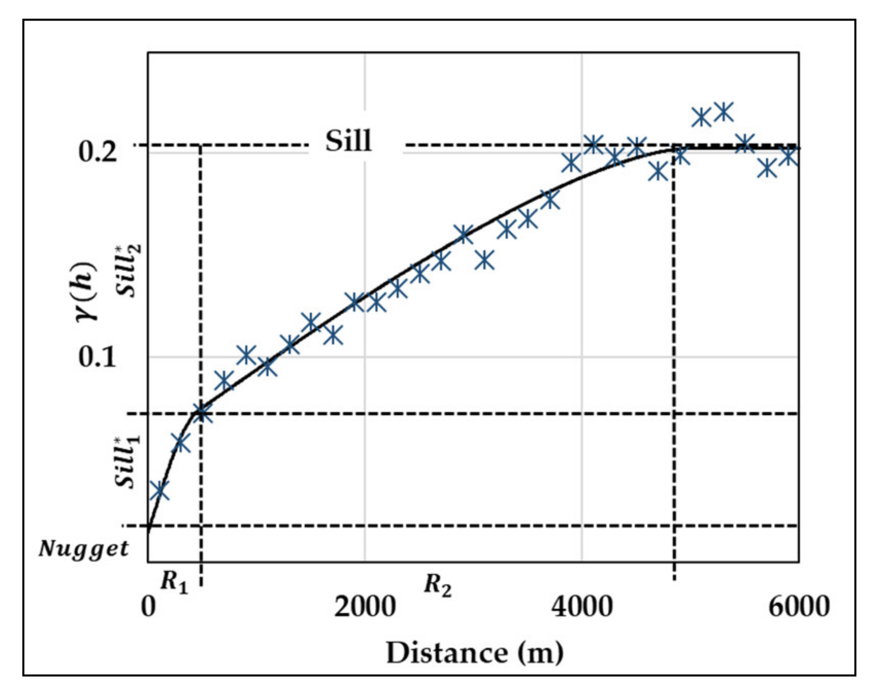
4.3. Modelling Spatial Variation: Variogram Analysis
5. Results
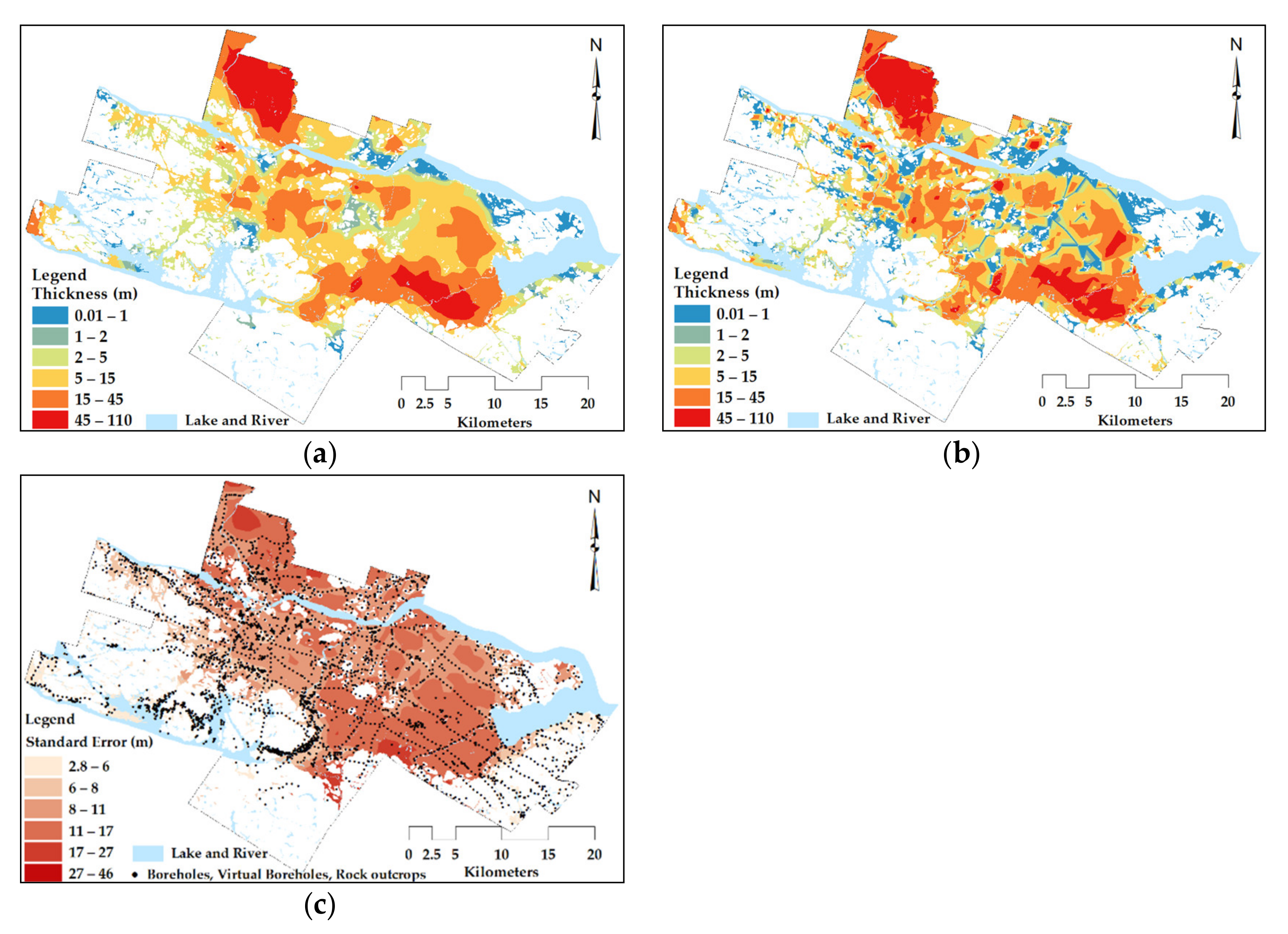
5.1. Construction of the Total Soil Thickness Map (Depth to Bedrock)
5.1.1. Spatial Interpolation
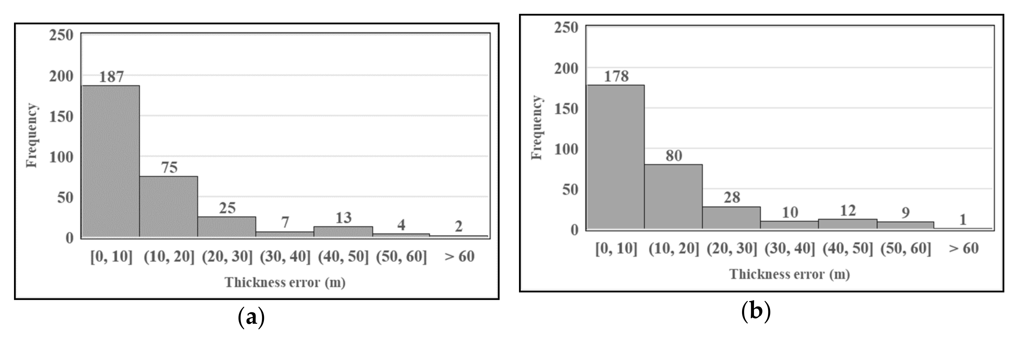
5.1.2. Validation
5.2. Determination of the Till Thickness Map
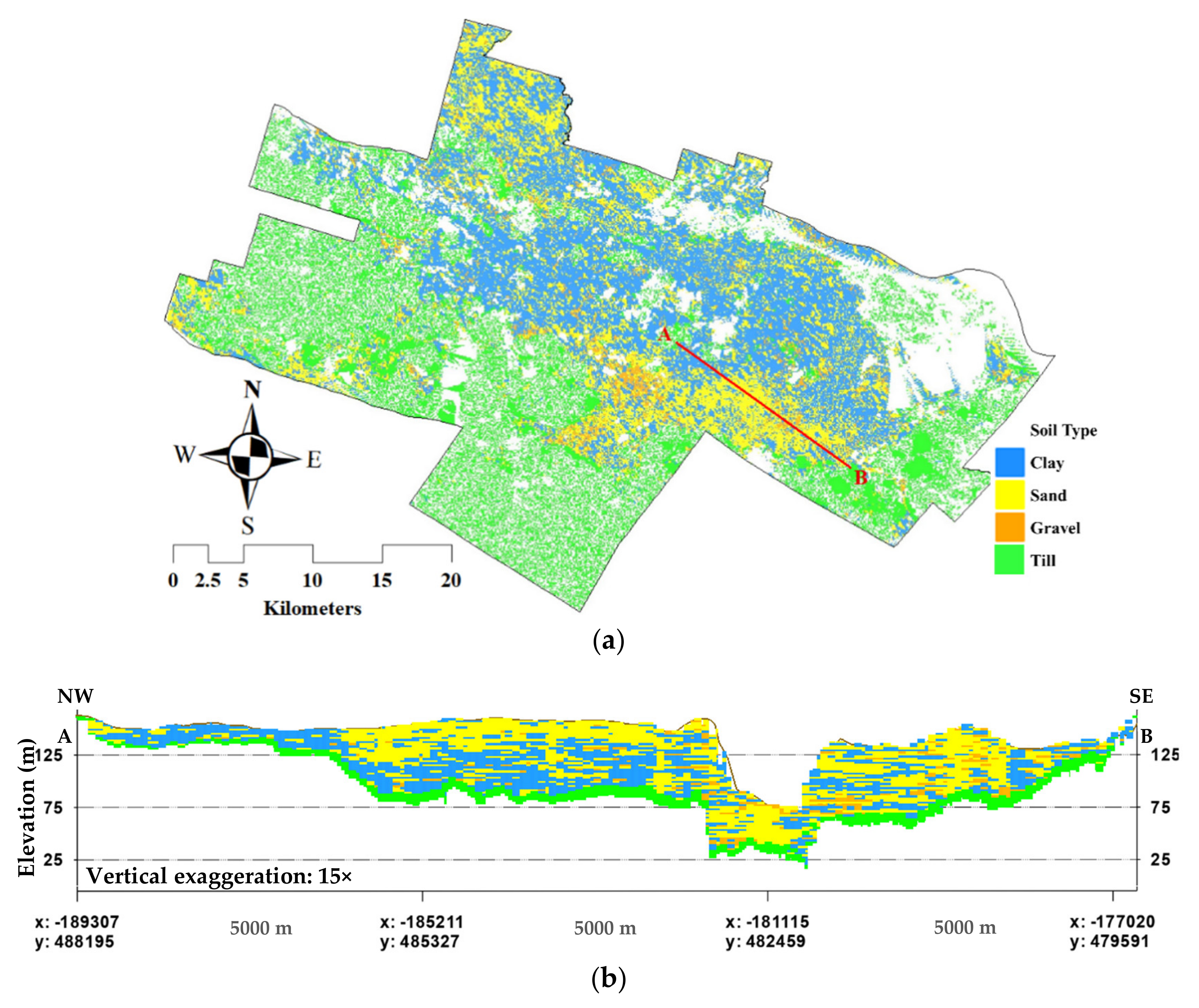
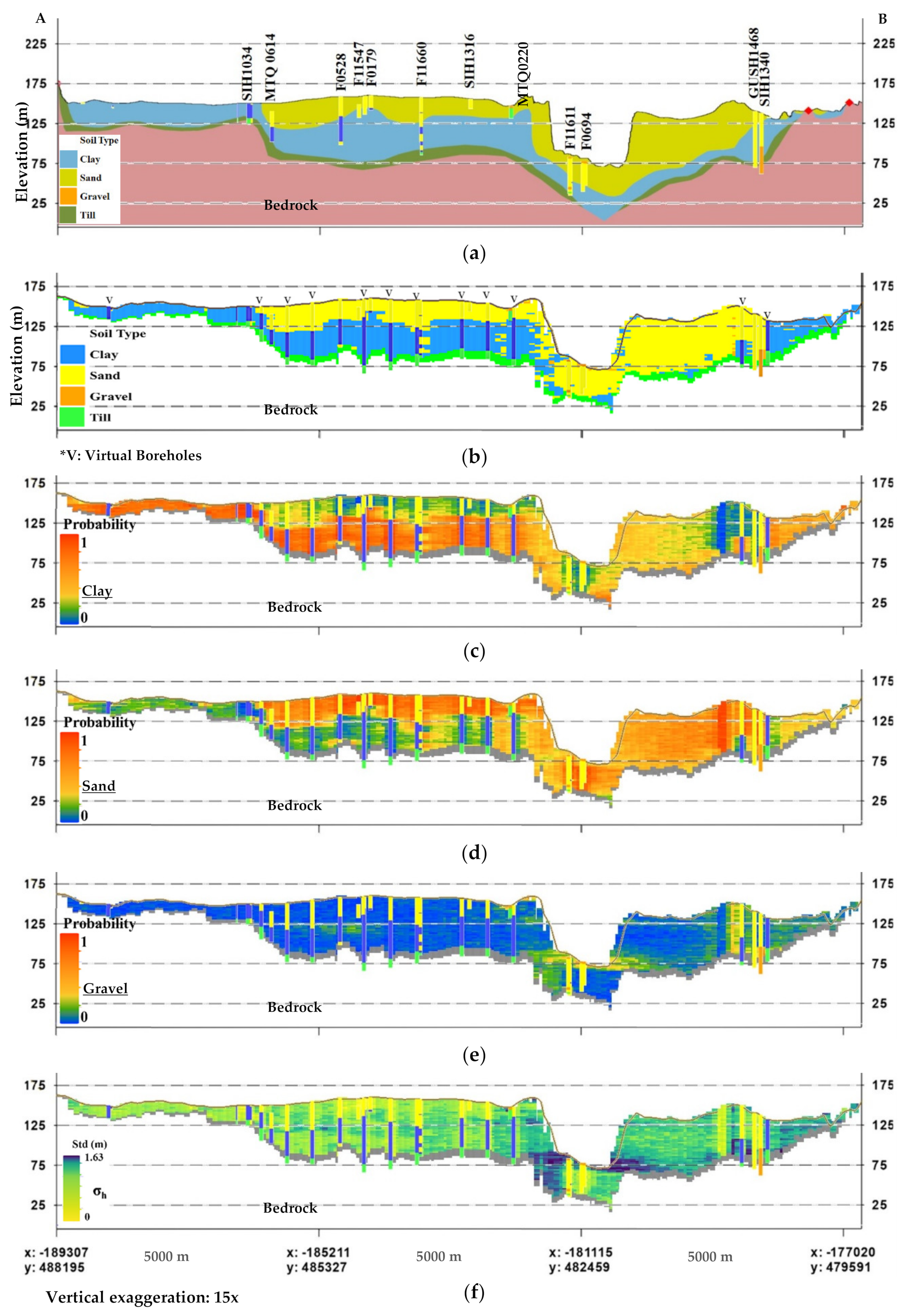
5.3. 3D Modelling of Discontinuous Soil Layers
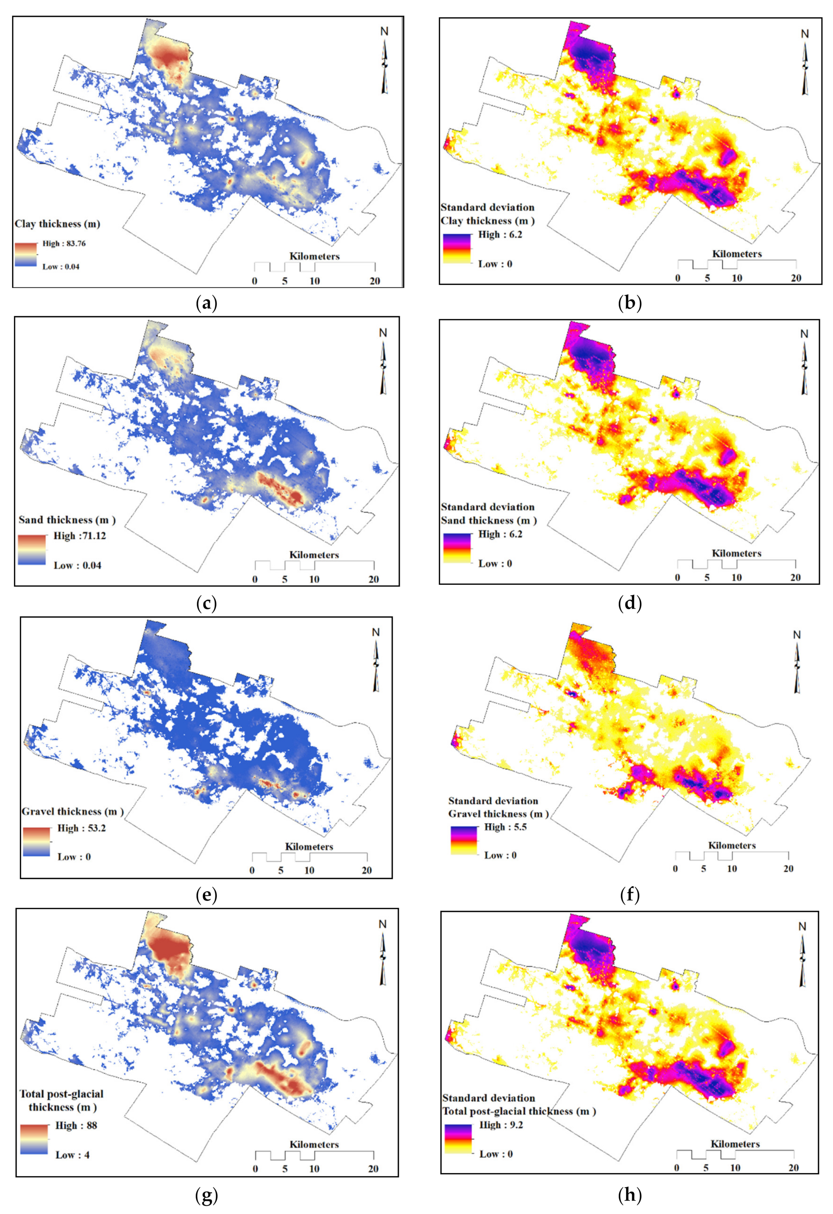
5.4. Thickness Maps of Discontinuous Soil Layers
6. Conclusions
Author Contributions
Funding
Acknowledgments
Conflicts of Interest
Nomenclature
| Variance of point values | |
| Covariance between measured samples | |
| Covariance between measured and unknown values | |
| EBK | Empirical Bayesian Kriging |
| fo | Fundamental site frequency of vibration |
| Binary indicator value at location and for category k | |
| Mean error | |
| Mean standardised error | |
| Mean square standardised error | |
| Root mean square error | |
| SIS | Sequential indicator simulation |
| TIN | Triangulated irregular network |
| To | Fundamental site period of vibration |
| u | Coordinates vector |
| Shear wave velocity | |
| Average shear wave velocity of the top 30 m | |
| Average shear wave velocity of the entire soil deposit | |
| Kriging weights | |
| Z() | Random variable at location |
| Experimental variogram | |
| Indicator variogram for category k | |
| Error variance of kriging |
References
- Elkateb, T.; Chalaturnyk, R.; Robertson, P.K. An overview of soil heterogeneity: Quantification and implications on geotechnical field problems. Can. Geotech. J. 2003, 40, 1–15. [Google Scholar] [CrossRef]
- Fenton, G.A. Estimation for Stochastic Soil Models. J. Geotech. Geoenviron. Eng. 1999, 125, 470–485. [Google Scholar] [CrossRef]
- Phoon, K.-K.; Kulhawy, F.H. Characterization of geotechnical variability. Can. Geotech. J. 1999, 36, 612–624. [Google Scholar] [CrossRef]
- Fenton, G.A.; Griffiths, D.V. Bearing-capacity prediction of spatially random c–ϕ soils. Can. Geotech. J. 2003, 40, 54–65. [Google Scholar] [CrossRef]
- Uzielli, M.; Vannucchi, G.; Phoon, K.K. Random field characterisation of stress-nomalised cone penetration testing parameters. Géotechnique 2005, 55, 3–20. [Google Scholar] [CrossRef]
- Wang, Y.; Zhao, T.; Phoon, K.-K. Direct simulation of random field samples from sparsely measured geotechnical data with consideration of uncertainty in interpretation. Can. Geotech. J. 2018, 55, 862–880. [Google Scholar] [CrossRef]
- Zhao, T.; Wang, Y. Non-parametric simulation of non-stationary non-gaussian 3D random field samples directly from sparse measurements using signal decomposition and Markov Chain Monte Carlo (MCMC) simulation. Reliab. Eng. Syst. Saf. 2020, 203, 107087. [Google Scholar] [CrossRef]
- Ferrari, F.; Apuani, T.; Giani, G. Rock Mass Rating spatial estimation by geostatistical analysis. Int. J. Rock Mech. Min. Sci. 2014, 70, 162–176. [Google Scholar] [CrossRef] [Green Version]
- Pinheiro, M.; Vallejos, J.; Miranda, T.; Emery, X. Geostatistical simulation to map the spatial heterogeneity of geomechanical parameters: A case study with rock mass rating. Eng. Geol. 2016, 205, 93–103. [Google Scholar] [CrossRef]
- Kring, K.; Chatterjee, S. Uncertainty quantification of structural and geotechnical parameter by geostatistical simulations applied to a stability analysis case study with limited exploration data. Int. J. Rock Mech. Min. Sci. 2020, 125, 104157. [Google Scholar] [CrossRef]
- Vessia, G.; Di Curzio, D.; Castrignanò, A. Modeling 3D soil lithotypes variability through geostatistical data fusion of CPT parameters. Sci. Total. Environ. 2020, 698, 134340. [Google Scholar] [CrossRef]
- Lee, R.L.; Bradley, B.A.; Ghisetti, F.C.; Thomson, E.M. Development of a 3D Velocity Model of the Canterbury, New Zealand, Region for Broadband Ground-Motion Simulation. Bull. Seism. Soc. Am. 2017, 107, 2131–2150. [Google Scholar] [CrossRef]
- Rohmer, O.; Bertrand, E.; Mercerat, E.; Régnier, J.; Pernoud, M.; Langlaude, P.; Alvarez, M. Combining borehole log-stratigraphies and ambient vibration data to build a 3D Model of the Lower Var Valley, Nice (France). Eng. Geol. 2020, 270, 105588. [Google Scholar] [CrossRef]
- Hallal, M.M.; Cox, B.R. An H/V geostatistical approach for building pseudo-3D Vs models to account for spatial variability in ground response analyses Part I: Model development. Earthq. Spectra 2021. [Google Scholar] [CrossRef]
- Rosset, P.; Bour-Belvaux, M.; Chouinard, L. Microzonation models for Montreal with respect to VS30. Bull. Earthq. Eng. 2014, 13, 2225–2239. [Google Scholar] [CrossRef]
- Nastev, M.; Parent, M.; Ross, M.; Howlett, D.; Benoit, N. Geospatial modelling of shear-wave velocity and fundamental site period of Quaternary marine and glacial sediments in the Ottawa and St. Lawrence Valleys, Canada. Soil Dyn. Earthq. Eng. 2016, 85, 103–116. [Google Scholar] [CrossRef]
- Foulon, T.; Saeidi, A.; Chesnaux, R.; Nastev, M.; Rouleau, A. Spatial distribution of soil shear-wave velocity and the fundamental period of vibration—A case study of the Saguenay region, Canada. Georisk Assess. Manag. Risk Eng. Syst. Geohazards 2017, 12, 74–86. [Google Scholar] [CrossRef]
- Myers, D.E. Spatial interpolation: An overview. Geoderma 1994, 62, 17–28. [Google Scholar] [CrossRef]
- Li, J.; Heap, A.D. Spatial interpolation methods applied in the environmental sciences: A review. Environ. Model. Softw. 2014, 53, 173–189. [Google Scholar] [CrossRef]
- Isaaks, E.H.; Srivastava, M.R. Applied Geostatistics; Oxford University Press: New York, NY, USA, 1989. [Google Scholar]
- Chiles, J.-P.; Delfiner, P. Geostatistics: Modeling Spatial Uncertainty; John Wiley & Sons: Hoboken, NJ, USA, 2009; Volume 497. [Google Scholar]
- Krivoruchko, K.; Gribov, A. Evaluation of empirical Bayesian kriging. Spat. Stat. 2019, 32, 100368. [Google Scholar] [CrossRef]
- Mirzaei, R.; Sakizadeh, M. Comparison of interpolation methods for the estimation of groundwater contamination in Andimeshk-Shush Plain, Southwest of Iran. Environ. Sci. Pollut. Res. 2015, 23, 2758–2769. [Google Scholar] [CrossRef]
- Giustini, F.; Ciotoli, G.; Rinaldini, A.; Ruggiero, L.; Voltaggio, M. Mapping the geogenic radon potential and radon risk by using Empirical Bayesian Kriging regression: A case study from a volcanic area of central Italy. Sci. Total. Environ. 2019, 661, 449–464. [Google Scholar] [CrossRef]
- Chesnaux, R.; Lambert, M.; Walter, J.; Dugrain, V.; Rouleau, A.; Daigneault, R. A simplified geographical information systems (GIS)-based methodology for modeling the topography of bedrock: Illustration using the Canadian Shield. Appl. Geomat. 2017, 9, 61–78. [Google Scholar] [CrossRef]
- Goovaerts, P. Geostatistics in soil science: State-of-the-art and perspectives. Geoderma 1999, 89, 1–45. [Google Scholar] [CrossRef]
- Deutsch, C.V. A sequential indicator simulation program for categorical variables with point and block data: BlockSIS. Comput. Geosci. 2006, 32, 1669–1681. [Google Scholar] [CrossRef]
- Deutsch, C.V.; Journel, A.G. GSLIB Geostatistical Software Library and User’s Guide, 2nd ed.; Oxford University Press: New York, NY, USA, 1997; 369p. [Google Scholar]
- Du Berger, R.; Roy, D.W.; Lamontagne, M.; Woussen, G.; North, R.G.; Wetmiller, R.J. The Saguenay (Quebec) earthquake of November 25, 1988: Seismologic data and geologic setting. Tectonophysics 1991, 186, 59–74. [Google Scholar] [CrossRef]
- Lamontagne, M. An Overview of Some Significant Eastern Canadian Earthquakes and Their Impacts on the Geological Environment, Buildings and the Public. Nat. Hazards 2002, 26, 55–68. [Google Scholar] [CrossRef]
- Davidson, A. Geological Map of the Grenville Province: Canada and Adjacent Parts of the United States of America. Map 1947A; Geological Survey of Canada: Quebec City, QC, Canada, 1998. [Google Scholar]
- LaSalle, P.; Tremblay, G. Dépôts Meubles Saguenay Lac Saint-Jean. Rapport 191; Ministère des Richesses naturelles du Québec: Quebec City, QC, USA, 1978; 61p. [Google Scholar]
- Daigneault, R.-A.; Cousineau, P.; Leduc, E.; Beaudoin, G.; Millette, S.; Horth, N.; Allard, G. Rapport Final sur les Travaux de Cartographie des Formations Superficielles Réalisés dans le Territoire Municipalisé du Saguenay-Lac-Saint-Jean; Ministère des Ressources naturelles et de la Faune du Québec: Quebec City, QC, Canada, 2011. [Google Scholar]
- CERM-PACES. Résultat du Programme d’Acquisition de Connaissances sur les Eaux Souterraines de la Région Saguenay-Lac-Saint-Jean. Chicoutimi: Centre d’Études sur les Ressources Minérales, Université du Québec à Chicoutimi. 2013. Available online: http://paces.uqac.ca/programme.html (accessed on 29 April 2021).
- Walter, J.; Rouleau, A.; Chesnaux, R.; Lambert, M.; Daigneault, R. Characterization of general and singular features of major aquifer systems in the Saguenay-Lac-Saint-Jean region. Can. Water Resour. J. 2017, 43, 75–91. [Google Scholar] [CrossRef]
- Liang, M.; Marcotte, D.; Benoit, N. A comparison of approaches to include outcrop information in overburden thickness estimation. Stoch. Environ. Res. Risk Assess. 2013, 28, 1733–1741. [Google Scholar] [CrossRef]
- Wu, C.; Wu, J.; Luo, Y.; Zhang, H.; Teng, Y.; DeGloria, S.D. Spatial interpolation of severely skewed data with several peak values by the approach integrating kriging and triangular irregular network interpolation. Environ. Earth Sci. 2011, 63, 1093–1103. [Google Scholar] [CrossRef]
- Remy, N.; Boucher, A.; Wu, J. Applied Geostatistics with SGeMS: A User’s Guide; Cambridge University Press: Cambridge, UK, 2009. [Google Scholar]
- Pilz, J.; Spöck, G. Why do we need and how should we implement Bayesian kriging methods. Stoch. Environ. Res. Risk Assess. 2007, 22, 621–632. [Google Scholar] [CrossRef]
- Krivoruchko, K. Empirical Bayesian Kriging; ESRI: Redlands, CA, USA, 2012; Available online: http://www.Esri.Com/News/Arcuser/1012/Empirical-Byesian-Kriging (accessed on 29 April 2021).


| Geological Unit | Real Borehole Data (%) | Virtual Logs (%) |
|---|---|---|
| Clay | 53.60% | 58.54% |
| Gravel | 6.80% | 2.06% |
| Sand | 35.66% | 18.37% |
| Till | 3.94% | 21.03% |
| Variables | Number of Structures | Model Properties Structure 1 | Model Properties Structure 2 | ||||
|---|---|---|---|---|---|---|---|
| Model Type | Anisotropy Axis (amax, amed, amin) | Model Parameters | Model Type | Anisotropy Axis (amax, amed, amin) | Model Parameters | ||
| Clay | 2 | Sp. | (135°,45°,90°) | Nugget: 0.01 R1: (375,212.5,75) Sill1 *: 0.18 | Ex. | (135°,45°,90°) | R2: (12825,4275,75) Sill2 *: 0.05 |
| Sand | 2 | Sp. | (135°,45°,90°) | Nugget: 0.02 R1: (412.5187.5,62.5) Sill1 *: 0.17 | Sp. | (0°,0°,90°) | R2: (12375,12375,62.5) Sill2 *: 0.03 |
| Gravel | 2 | Sp. | - | Nugget: 0.01 R1: (150,150,150) Sill1 *: 0.026 | Ga. | (0°,0°,90°) | R2: (4600,4600,150) Sill2 *: 0.015 |
| ME (m) | RMSE (m) | MSE | MSSE |
|---|---|---|---|
| 0.05 | 8.94 | 0.01 | 0.94 |
| Thickness Error | TIN | EBK |
|---|---|---|
| Mean (m) | 12.2 | 11.8 |
| Sum (m) | 3889.8 | 3682.6 |
| Error count (boreholes) | 318 | 313 |
Publisher’s Note: MDPI stays neutral with regard to jurisdictional claims in published maps and institutional affiliations. |
© 2021 by the authors. Licensee MDPI, Basel, Switzerland. This article is an open access article distributed under the terms and conditions of the Creative Commons Attribution (CC BY) license (https://creativecommons.org/licenses/by/4.0/).
Share and Cite
Salsabili, M.; Saeidi, A.; Rouleau, A.; Nastev, M. 3D Probabilistic Modelling and Uncertainty Analysis of Glacial and Post-Glacial Deposits of the City of Saguenay, Canada. Geosciences 2021, 11, 204. https://0-doi-org.brum.beds.ac.uk/10.3390/geosciences11050204
Salsabili M, Saeidi A, Rouleau A, Nastev M. 3D Probabilistic Modelling and Uncertainty Analysis of Glacial and Post-Glacial Deposits of the City of Saguenay, Canada. Geosciences. 2021; 11(5):204. https://0-doi-org.brum.beds.ac.uk/10.3390/geosciences11050204
Chicago/Turabian StyleSalsabili, Mohammad, Ali Saeidi, Alain Rouleau, and Miroslav Nastev. 2021. "3D Probabilistic Modelling and Uncertainty Analysis of Glacial and Post-Glacial Deposits of the City of Saguenay, Canada" Geosciences 11, no. 5: 204. https://0-doi-org.brum.beds.ac.uk/10.3390/geosciences11050204