
Laboratory Investigation of Hydraulic Fracture Behavior of Unconventional Reservoir Rocks

 , , ,
, , ,
Abstract
:1. Introduction
2. Materials and Methods
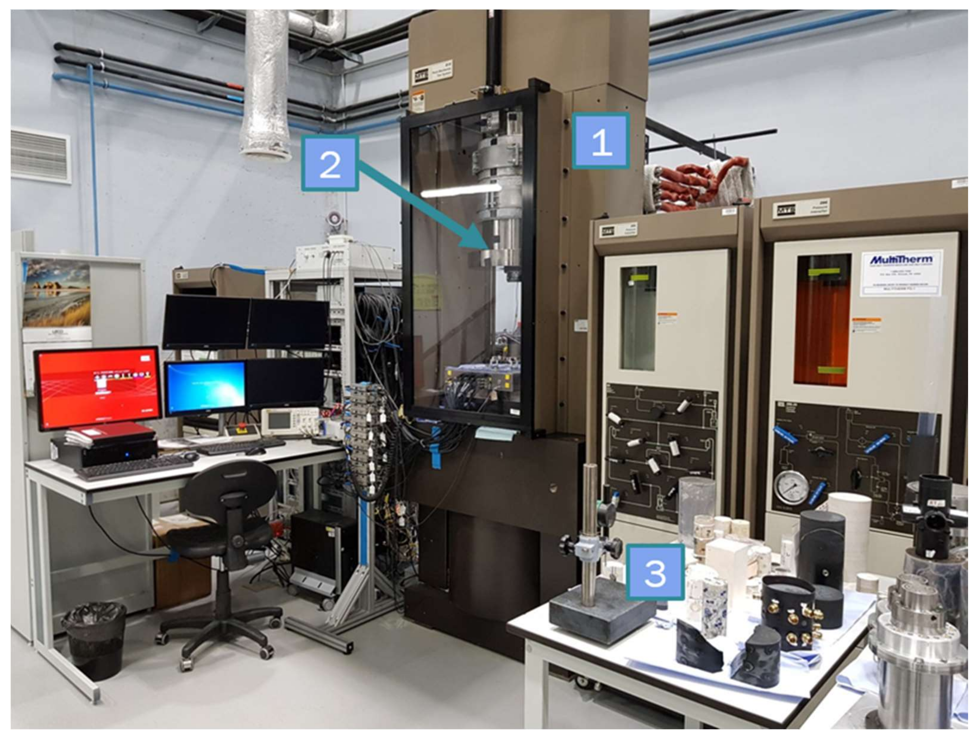
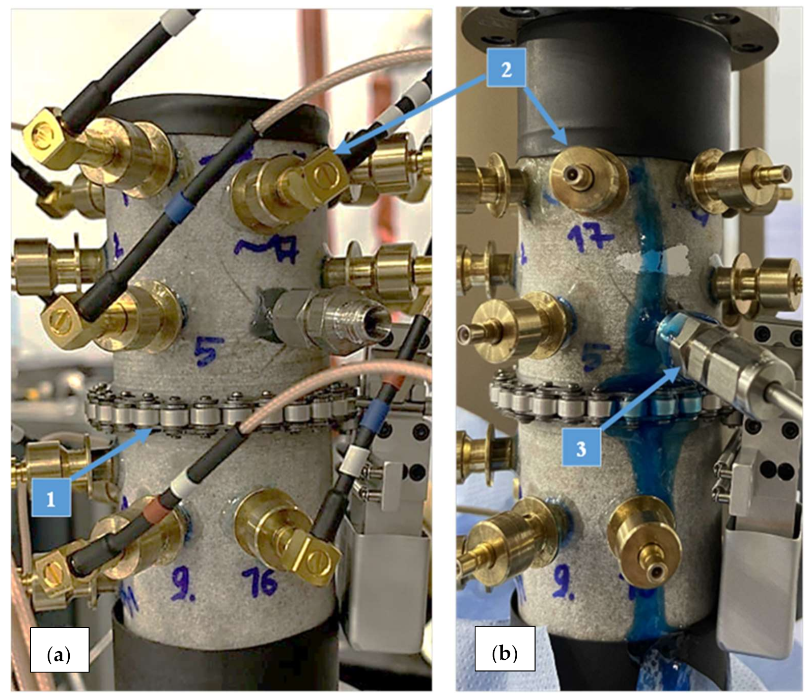
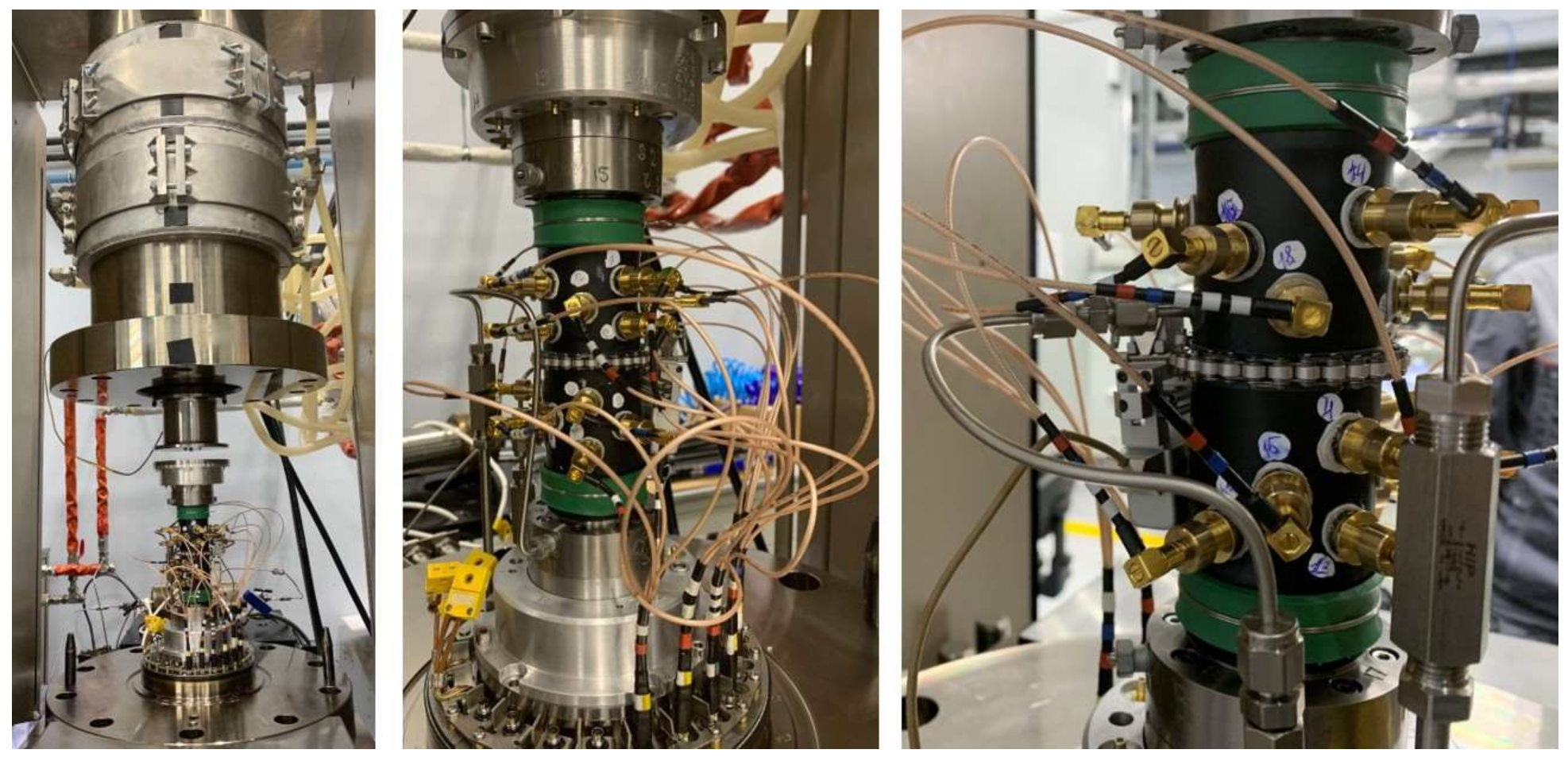
2.1. Experimental Setup
2.2. Experimental Method and Specimen Preparation
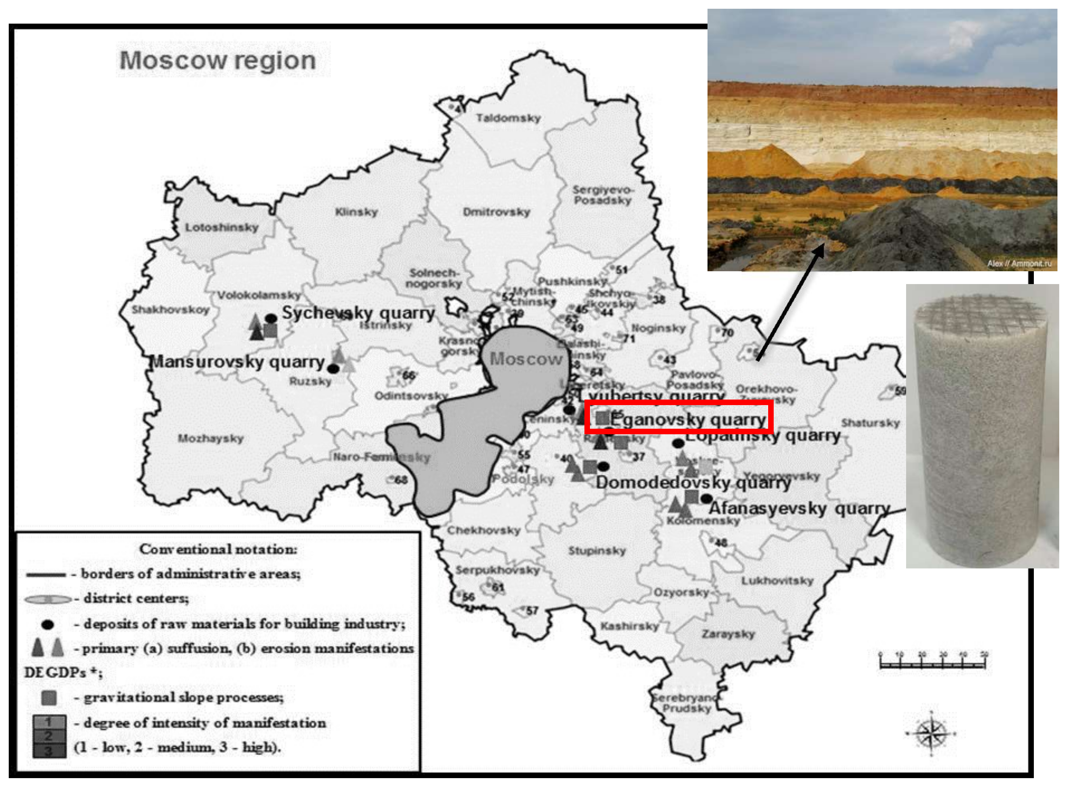
2.2.1. Characterization of a Sandstone Sample and Preparation for Testing
2.2.2. Characterization of Shale-Like Rock Samples and Preparation for Testing
3. Results
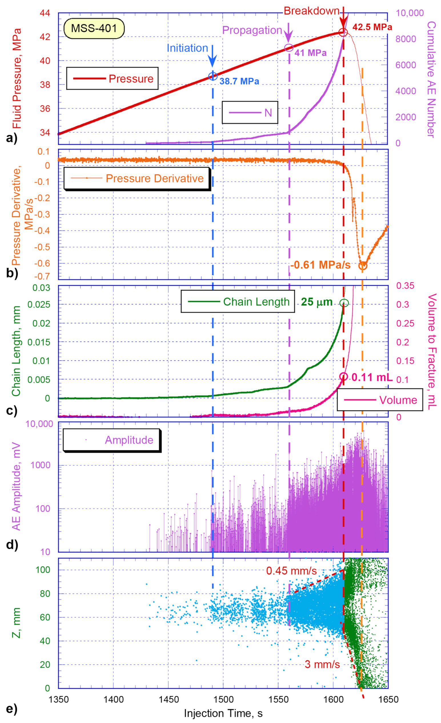
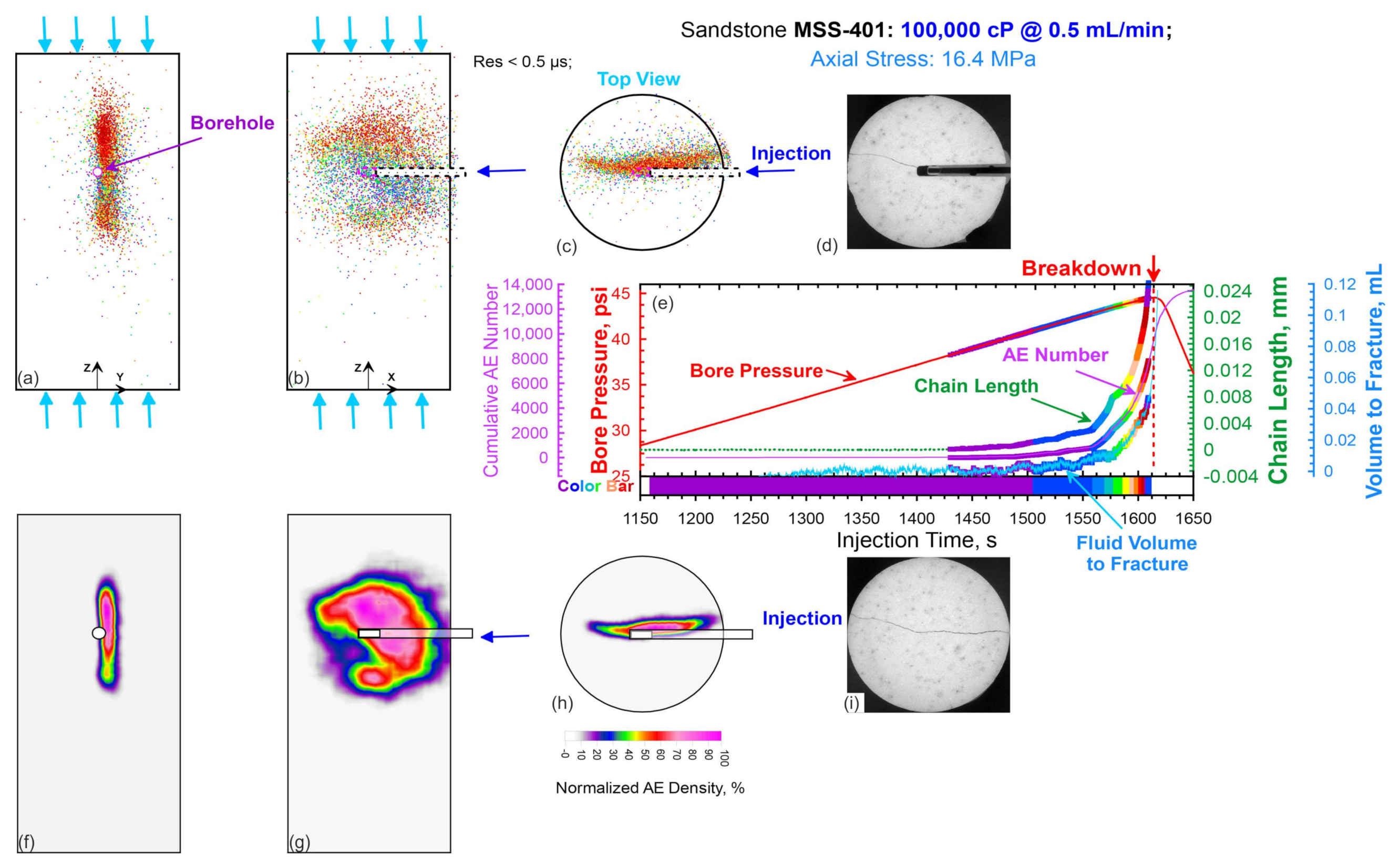
3.1. Propagation of Hydraulic Fracture in Sandstone
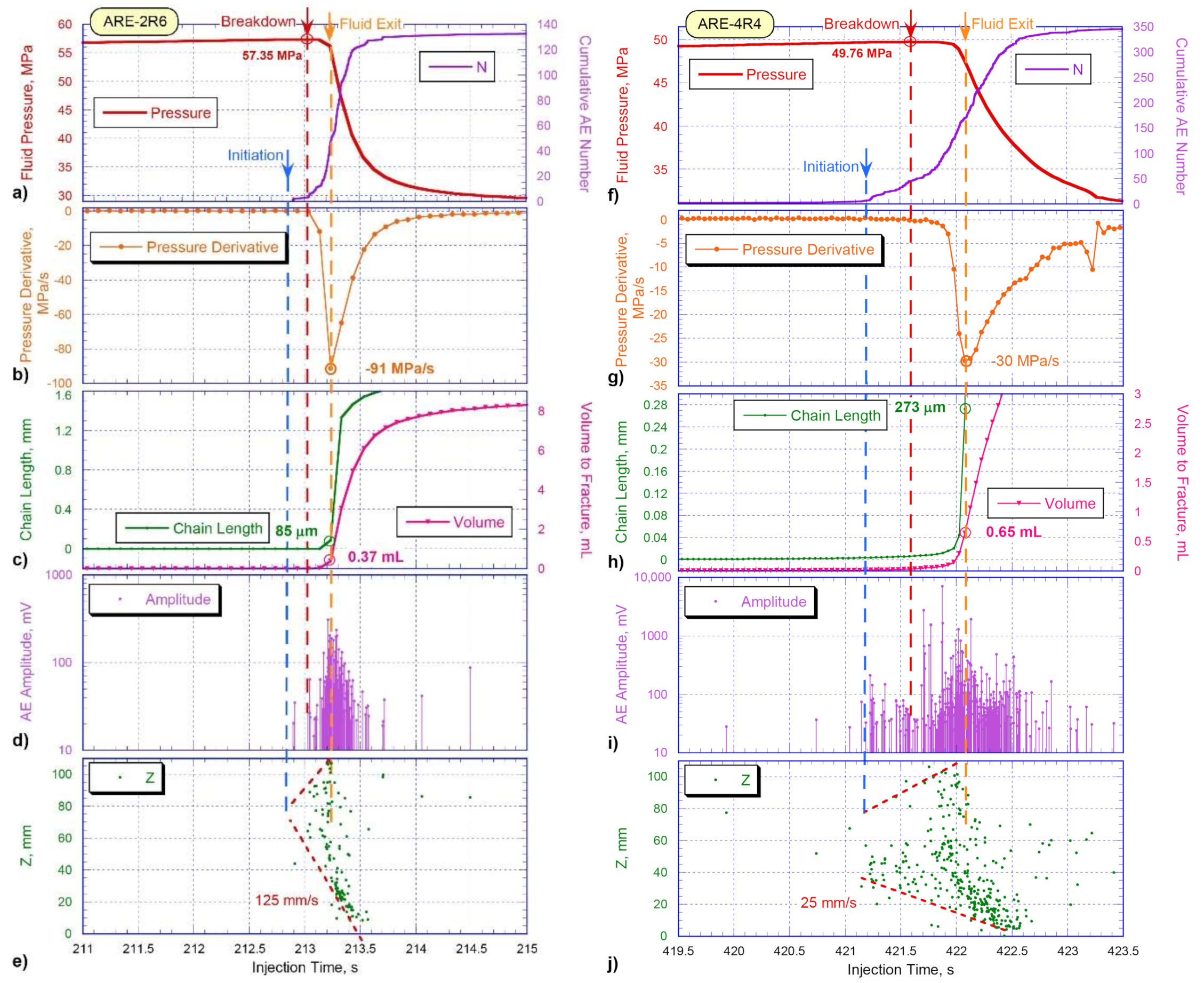
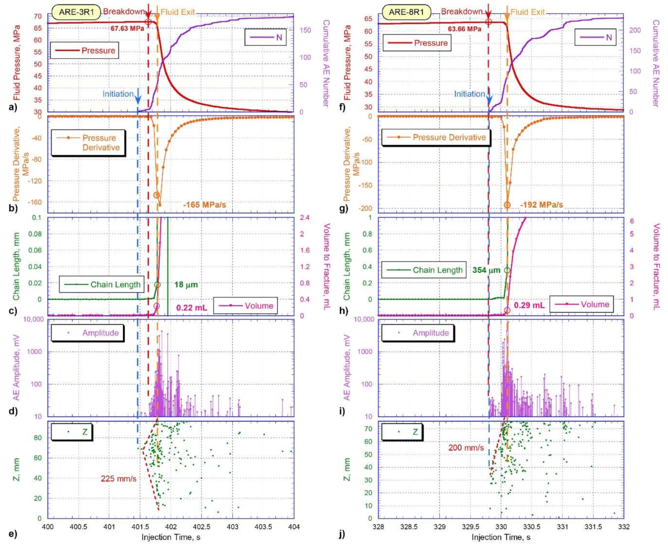
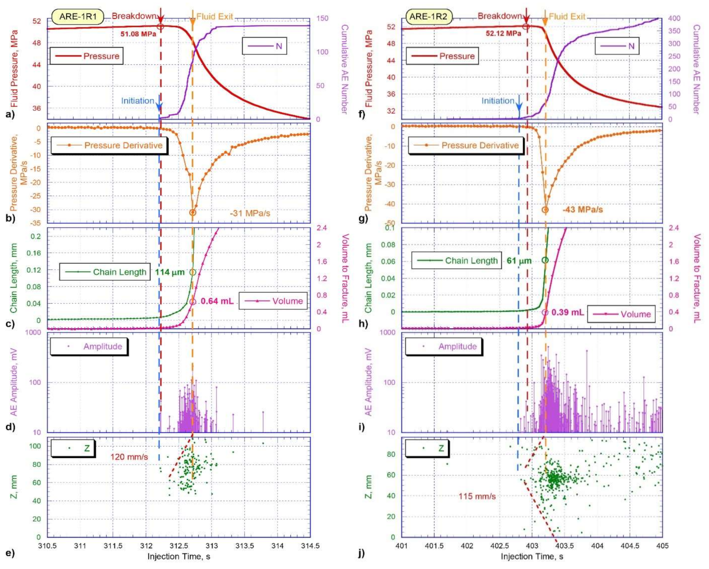
3.2. Comparison of Geomechanical and Acoustic Parameters of Testing Samples of Shale-Like Rocks
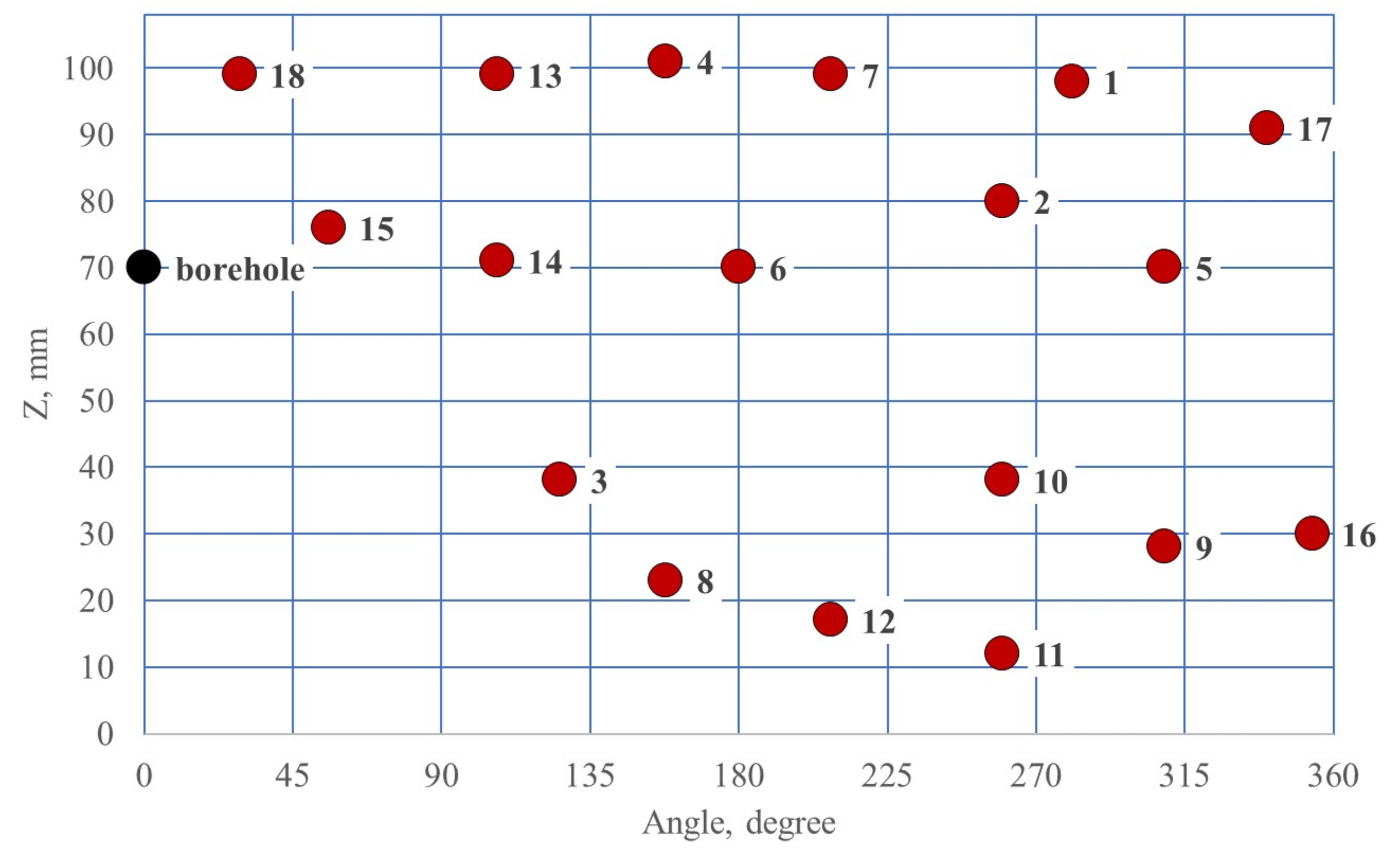
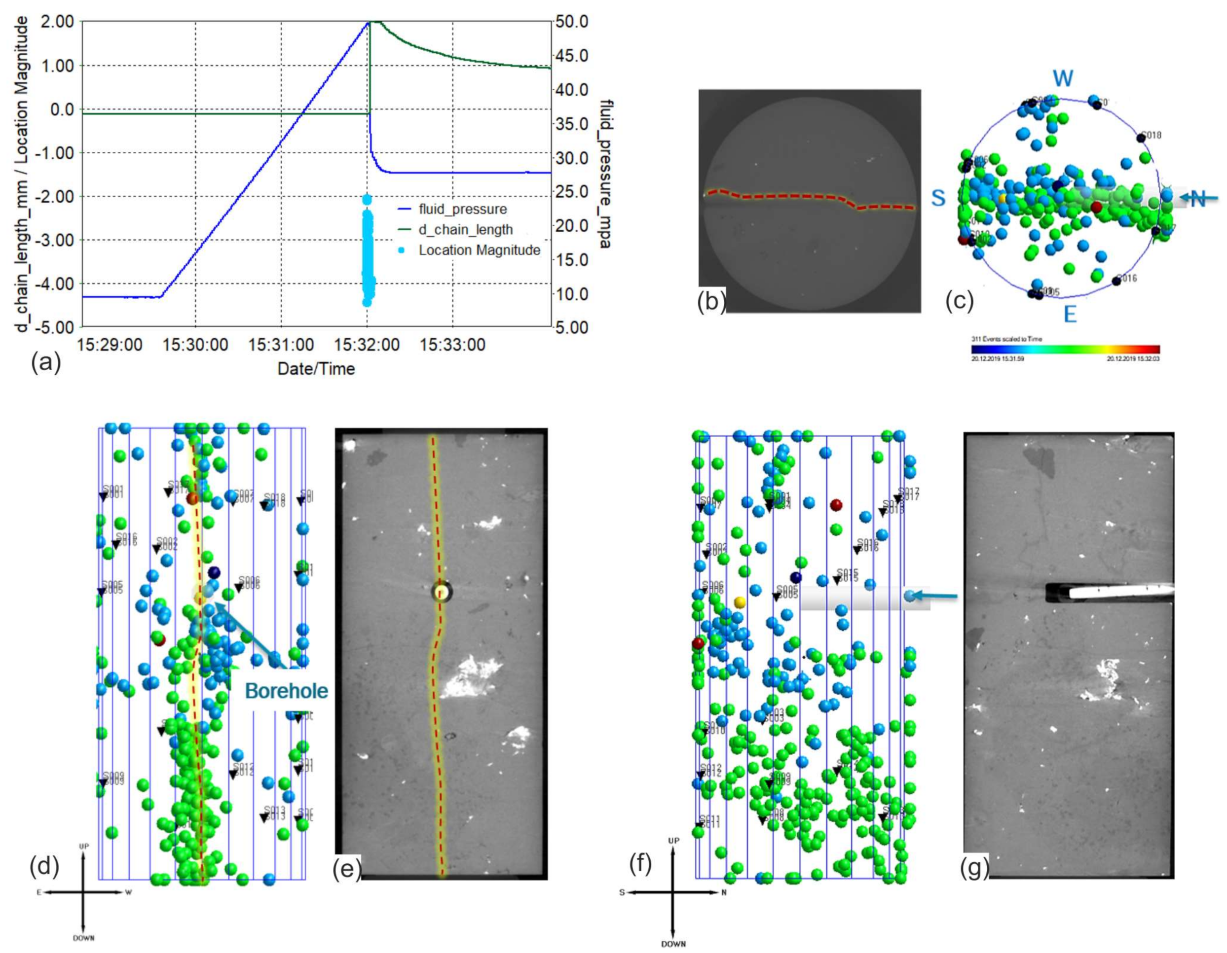
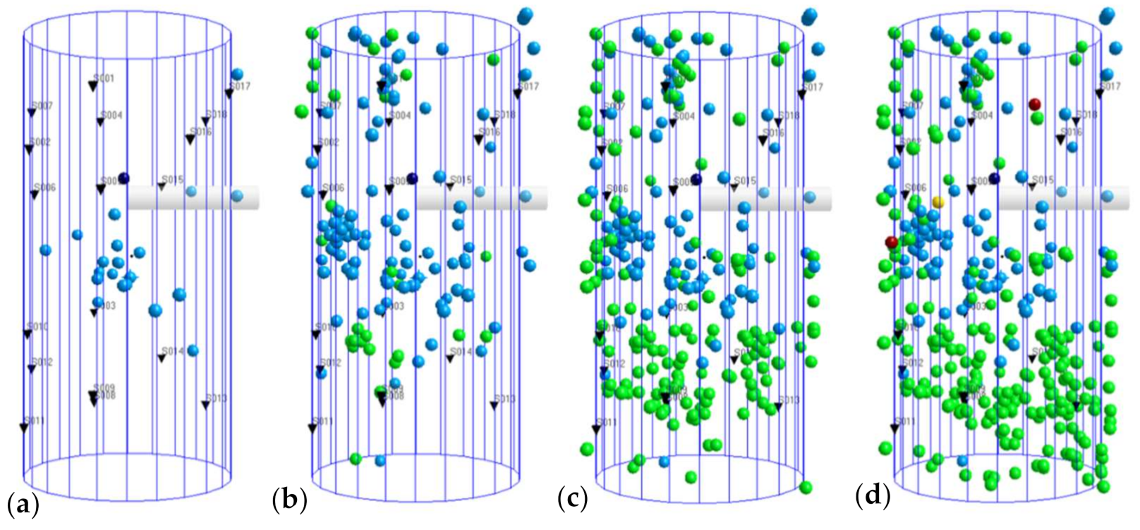
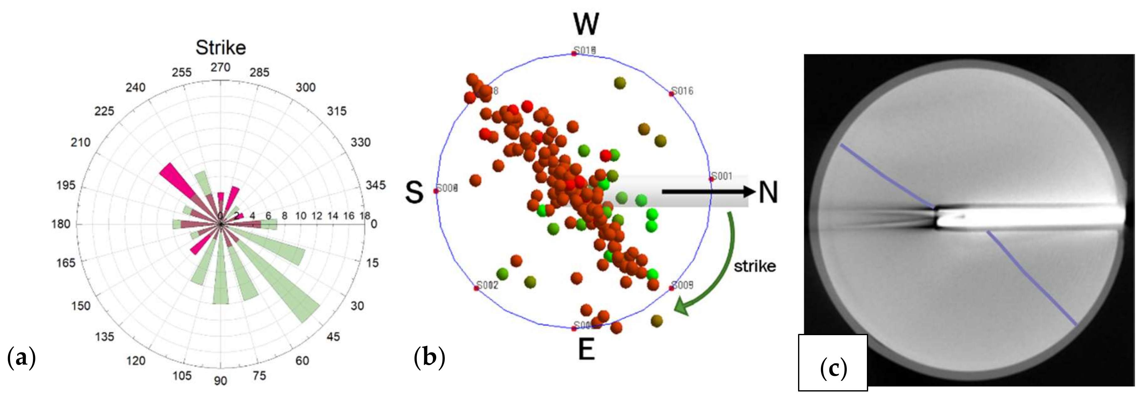
3.3. Three-Dimensional Localization of AE Events of Shale-Like Rocks
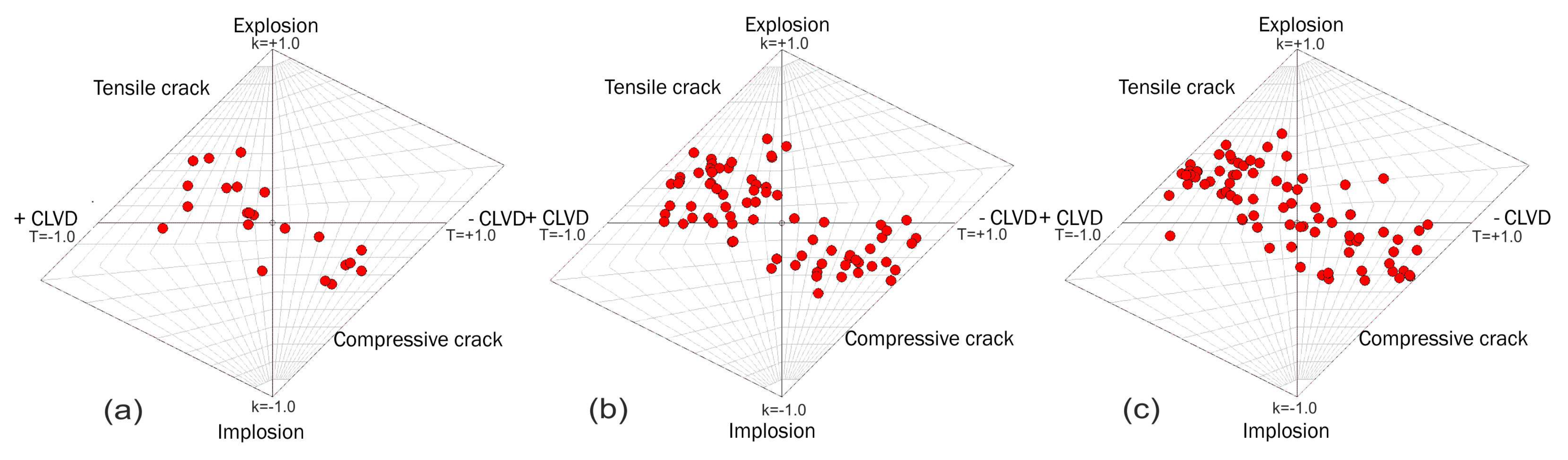
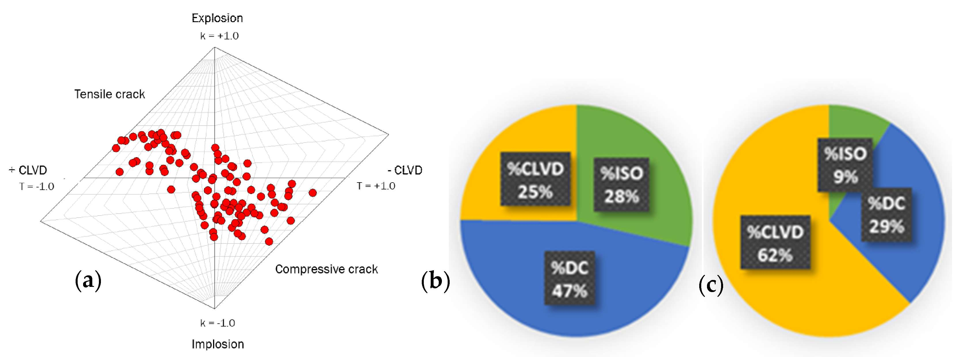
3.4. Analysis of Moment Tensor Inversion of Shale-Like Rocks
4. Discussion
5. Conclusions
Author Contributions
Funding
Data Availability Statement
Acknowledgments
Conflicts of Interest
References
- Soeder, D.J. The successful development of gas and oil resources from shales in North America. J. Pet. Sci. Eng. 2018, 163, 399–420. [Google Scholar] [CrossRef]
- Henderson, J. Tight Oil Developments in Russia; Oxford Institute for Energy Studies: Oxford, UK, 2013. [Google Scholar]
- Denney, D. Thirty Years of Gas-Shale Fracturing: What Have We Learned? J. Pet. Technol. 2010, 62, 88–90. [Google Scholar] [CrossRef]
- Yi, P.; Haifeng, F.; Mingyue, C.; Yunzhi, L.; Yun, X.; Yongjun, L.; Xing, W.; Yonghui, W. What Do Hydraulic Fractures Look Like in Different Types of Reservoirs: Implications from a Series of Large-Scale Polyaxial Hydraulic Fracturing Experiments from Conventional to Unconventional. In Proceedings of the 7th Unconventional Resources Technology Conference, Denver, CO, USA, 22–24 July 2019; pp. 1–14. [Google Scholar] [CrossRef]
- Heng, S.; Li, X.; Zhang, X.; Li, Z. Mechanisms for the control of the complex propagation behaviour of hydraulic fractures in shale. J. Pet. Sci. Eng. 2021, 200, 108417. [Google Scholar] [CrossRef]
- Strpić, K.; Miličević, M.; Kurevija, T. Development of Tight Oil Resources in USA: Profitability of Exploitation and Effect of Macroeconomic Indicators in Volatile Oil Price Environment. Rud. Geološko Naft. Zb. 2017, 32, 23–33. [Google Scholar] [CrossRef] [Green Version]
- Guo, F.; Morgenstern, N.; Scott, J. An experimental investigation into hydraulic fracture propagation—Part 2. Single well tests. Int. J. Rock Mech. Min. Sci. Géoméch. Abstr. 1993, 30, 189–202. [Google Scholar] [CrossRef]
- Zoback, M.; Rummel, F.; Jung, R.; Raleigh, C. Laboratory hydraulic fracturing experiments in intact and pre-fractured rock. Int. J. Rock Mech. Min. Sci. Géoméch. Abstr. 1977, 14, 49–58. [Google Scholar] [CrossRef]
- Patel, S.; Sondergeld, C.; Rai, C. Laboratory studies of hydraulic fracturing by cyclic injection. Int. J. Rock Mech. Min. Sci. 2017, 95, 8–15. [Google Scholar] [CrossRef]
- Akrad, O.M.; Miskimins, J.L.; Prasad, M. The Effects of Fracturing Fluids on Shale Rock Mechanical Properties and Proppant Embedment. Days 2011, 3, 2245–2256. [Google Scholar] [CrossRef] [Green Version]
- Zhang, J.; Kamenov, A.; Zhu, D.; Hill, A.D. Laboratory Measurement of Hydraulic-Fracture Conductivities in the Barnett Shale. SPE Prod. Oper. 2014, 29, 216–227. [Google Scholar] [CrossRef]
- Fisher, K.; Warpinski, N. Hydraulic-Fracture-Height Growth: Real Data. SPE Prod. Oper. 2012, 27, 8–19. [Google Scholar] [CrossRef]
- Liang, Y.; Cheng, Y.; Zou, Q.; Wang, W.; Ma, Y.; Li, Q. Response characteristics of coal subjected to hydraulic fracturing: An evaluation based on real-time monitoring of borehole strain and acoustic emission. J. Nat. Gas Sci. Eng. 2017, 38, 402–411. [Google Scholar] [CrossRef]
- Stanchits, S.; Burghardt, J.; Surdi, A. Hydraulic Fracturing of Heterogeneous Rock Monitored by Acoustic Emission. Rock Mech. Rock Eng. 2015, 48, 2513–2527. [Google Scholar] [CrossRef]
- Chen, Y.; Nagaya, Y.; Ishida, T. Observations of Fractures Induced by Hydraulic Fracturing in Anisotropic Granite. Rock Mech. Rock Eng. 2015, 48, 1455–1461. [Google Scholar] [CrossRef]
- Stoeckhert, F.; Molenda, M.; Brenne, S.; Alber, M. Fracture propagation in sandstone and slate–Laboratory experiments, acoustic emissions and fracture mechanics. J. Rock Mech. Geotech. Eng. 2015, 7, 237–249. [Google Scholar] [CrossRef] [Green Version]
- Kolawole, O.; Ispas, I. Interaction between hydraulic fractures and natural fractures: Current status and prospective directions. J. Pet. Explor. Prod. Technol. 2020, 10, 1613–1634. [Google Scholar] [CrossRef] [Green Version]
- Li, Q.; Xing, H.; Liu, J.; Liu, X. A review on hydraulic fracturing of unconventional reservoir. Petroleum 2015, 1, 8–15. [Google Scholar] [CrossRef] [Green Version]
- Stanchits, S.; Surdi, A.; Gathogo, P.; Edelman, E.; Suarez-Rivera, R. Onset of Hydraulic Fracture Initiation Monitored by Acoustic Emission and Volumetric Deformation Measurements. Rock Mech. Rock Eng. 2014, 47, 1521–1532. [Google Scholar] [CrossRef]
- Wasantha, P.L.P.; Ranjith, P.; Zhang, Q.; Xu, T. Do joint geometrical properties influence the fracturing behaviour of jointed rock? An investigation through joint orientation. Géoméch. Geophys. Geo-energy Geo-resour. 2015, 1, 3–14. [Google Scholar] [CrossRef] [Green Version]
- Huang, B.; Li, P. Experimental Investigation on the Basic Law of the Fracture Spatial Morphology for Water Pressure Blasting in a Drillhole Under True Triaxial Stress. Rock Mech. Rock Eng. 2015, 48, 1699–1709. [Google Scholar] [CrossRef]
- Zhu, Q.; Feng, Y.; Cai, M.; Liu, J.; Wang, H. Interpretation of the extent of hydraulic fracturing for rockburst prevention using microseismic monitoring data. J. Nat. Gas Sci. Eng. 2017, 38, 107–119. [Google Scholar] [CrossRef]
- Chen, L.-H.; Chen, W.-C.; Chen, Y.-C.; Benyamin, L.; Li, A.-J. Investigation of Hydraulic Fracture Propagation Using a Post-Peak Control System Coupled with Acoustic Emission. Rock Mech. Rock Eng. 2014, 48, 1233–1248. [Google Scholar] [CrossRef]
- Li, B.Q.; da Silva, B.G.; Einstein, H. Laboratory hydraulic fracturing of granite: Acoustic emission observations and interpretation. Eng. Fract. Mech. 2019, 209, 200–220. [Google Scholar] [CrossRef]
- Zhai, H.; Chang, X.; Wang, Y.; Lei, X.; Xue, Z. Analysis of acoustic emission events induced during stress unloading of a hydraulic fractured Longmaxi shale sample. J. Pet. Sci. Eng. 2020, 189, 106990. [Google Scholar] [CrossRef]
- Lavrusevich, A.; Abene, A.; Lavrusevich, I. Geoecological aspects of technogenic impact on the territory of raw materials production for construction. MATEC Web Conf. 2019, 265, 06013. [Google Scholar] [CrossRef]
- Stanchits, S.A. Anisotropic Changes in P-Wave Velocity and Attenuation during Deformation and Fluid Infiltration of Granite. Bull. Seism. Soc. Am. 2003, 93, 1803–1822. [Google Scholar] [CrossRef]
- Stanchits, S.; Vinciguerra, S.; Dresen, G. Ultrasonic Velocities, Acoustic Emission Characteristics and Crack Damage of Basalt and Granite. Pure Appl. Geophys. PAGEOPH 2006, 163, 975–994. [Google Scholar] [CrossRef]
- Stanchits, S.; Mayr, S.; Shapiro, S.; Dresen, G. Fracturing of porous rock induced by fluid injection. Tectonophysics 2011, 503, 129–145. [Google Scholar] [CrossRef]
- Leonard, M.; Kennett, B. Multi-component autoregressive techniques for the analysis of seismograms. Phys. Earth Planet. Inter. 1999, 113, 247–263. [Google Scholar] [CrossRef]
- Nelder, J.A.; Mead, R. A Simplex Method for Function Minimization. Comput. J. 1965, 7, 308–313. [Google Scholar] [CrossRef]
- Punanova, S.A.; Chakhmakhchev, V.A.; Agafonova, Z.G.; Kukushkina, Z.P.; Gordadze, T.I. Oil Geochemistry of Subsalt Deposits of the Western Caspian Foundation, Geol. Oil Gas, No. 7, 1996. Available online: http://www.geolib.ru/OilGasGeo/1996/07/Stat/stat05.html (accessed on 14 July 2021). (In Russian).
- Ostroukhov, S.B.; Tsygankova, V.A.; Popova, P.F.; Kruk, P.N. On the genesis of oil and gas bearing subsalt lower artinskian deposits of the western Caspian. Subsurf. Resour. Volga Casp. Reg. 2019. [Google Scholar] [CrossRef]
- Mikhal’kova, V.N.; Brazhnikov, O.G.; Beresfetskaya, A.M. Selecting the Trends of Searching for Oil and Gas Deposits within the Western Part of the Precaspian Depression, Geol. Oil Gas, No. 5, 1990. Available online: http://geolib.narod.ru/Journals/OilGasGeo/1990/05/Stat/03/stat03.html (accessed on 14 July 2021). (In Russian).
- Gabnasyrov, A.V.; Lyadova, N.A.; Putilov, I.S.; Solovyev, S.I. Domanik Shale Oil: Unlocking Potential. In Proceedings of the All Days, Moscow, Russia, 24–26 October 2016; Society of Petroleum Engineers (SPE): Moscow, Russia, 2016; pp. 622–637. [Google Scholar]
- Lockner, D.A.; Byerlee, J.D.; Kuksenko, V. Observations of quasistatic fault growth from acoustic emissions. In International Geophysics; Academic Press: Cambridge, MA, USA, 1992; Volume 51, pp. 3–31. [Google Scholar]
- Durney, D.W. An application of normal mode theory to the retrieval of structural parameters and source mechanisms from seismic spectra. Philos. Trans. R. Soc. London. Ser. A Math. Phys. Sci. 1975, 278, 187–269. [Google Scholar] [CrossRef]
- Jia, Q.S.; Wong, R.C.K.; Eaton, D.W.; Eyre, T.S. Investigating fracture growth and source mechanisms in shale using acoustic emission technique. Proceeding of the 52nd U.S. Rock Mechanics/Geomechanic Symposium, Seattle, WA, USA, 17–20 June 2018. [Google Scholar]
- InSite Seismic Processor: Technical Appendix, 2021, Applied Seismology Consultants. Available online: https://www.appliedseismology.co.uk/support/resources/ (accessed on 14 July 2021).
- Hudson, J.A.; Pearce, R.G.; Rogers, R.M. Source type plot for inversion of the moment tensor. J. Geophys. Res. Space Phys. 1989, 94, 765–774. [Google Scholar] [CrossRef] [Green Version]
- Chapman, C.H.; Leaney, W.S. A new moment-tensor decomposition for seismic events in anisotropic media. Geophys. J. Int. 2011, 188, 343–370. [Google Scholar] [CrossRef] [Green Version]
- Aki, K.; Richards, P.G. Quantitative Seismology, 2nd ed.; University Science Books: Sausalito, CA, USA, 2009. [Google Scholar]
- Stanchits, S.; Surdi, A.; Edelman, E.; Suarez-Rivera, R. Acoustic Emission and Ultrasonic Transmission Monitoring of Hydraulic Fracture Initiation and Growth in Rock Samples. In Proceeding of the 46th U.S. Rock Mechanics/Geomechanics Symposium, Chicago, IL, USA, 24–27 June 2012; pp. 12–15. [Google Scholar]


| Sample | Length, mm | Diameter, mm | Density, g/cm3 | Porosity, % | Gas Permeability, mD | Young’s Modulus E, GPa | Poisson’s Ratio |
|---|---|---|---|---|---|---|---|
| MSS-401 | 107.99 | 49.22 | 2.54 | 3.65 | 1.59 | 72.93 | 0.15 |
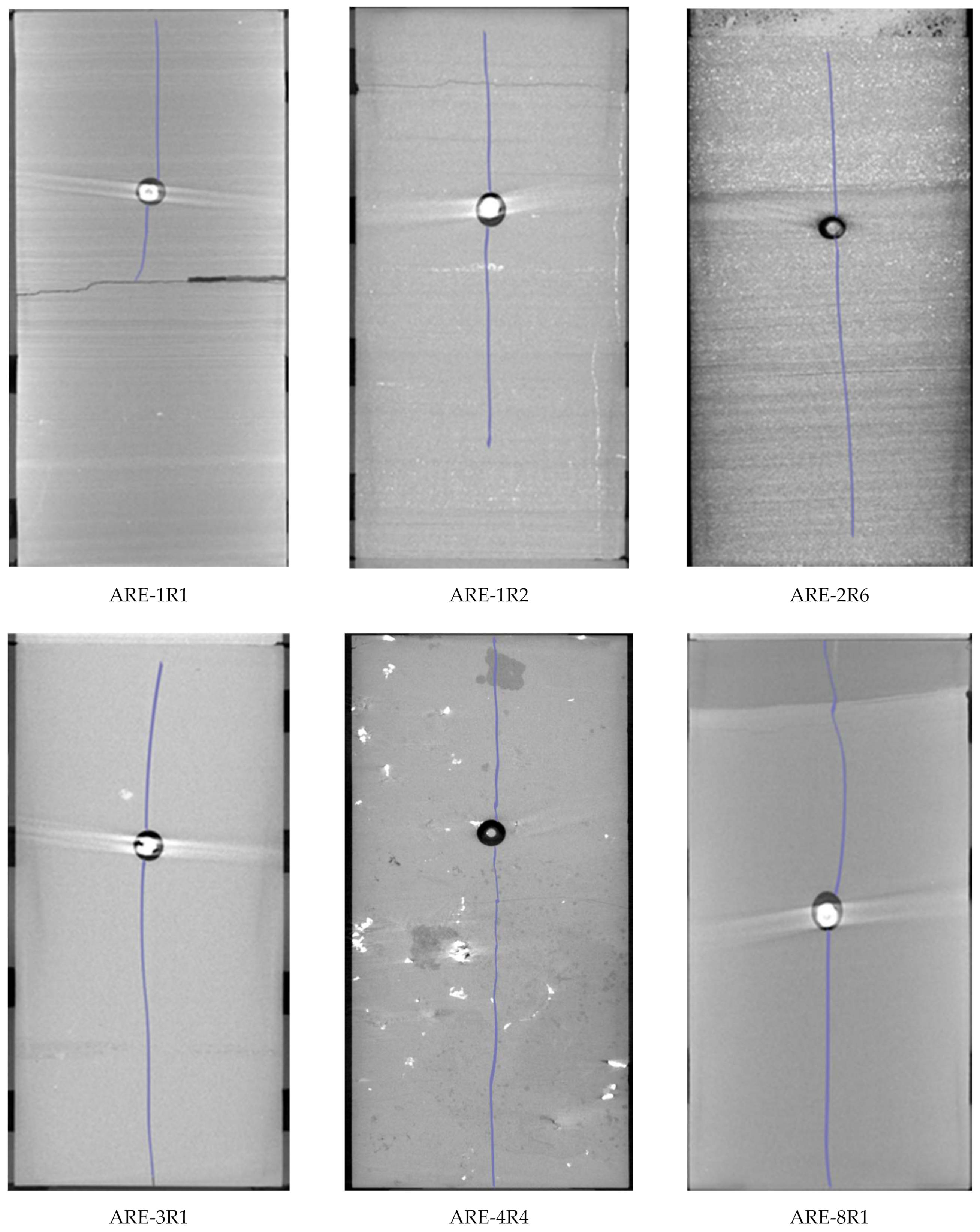
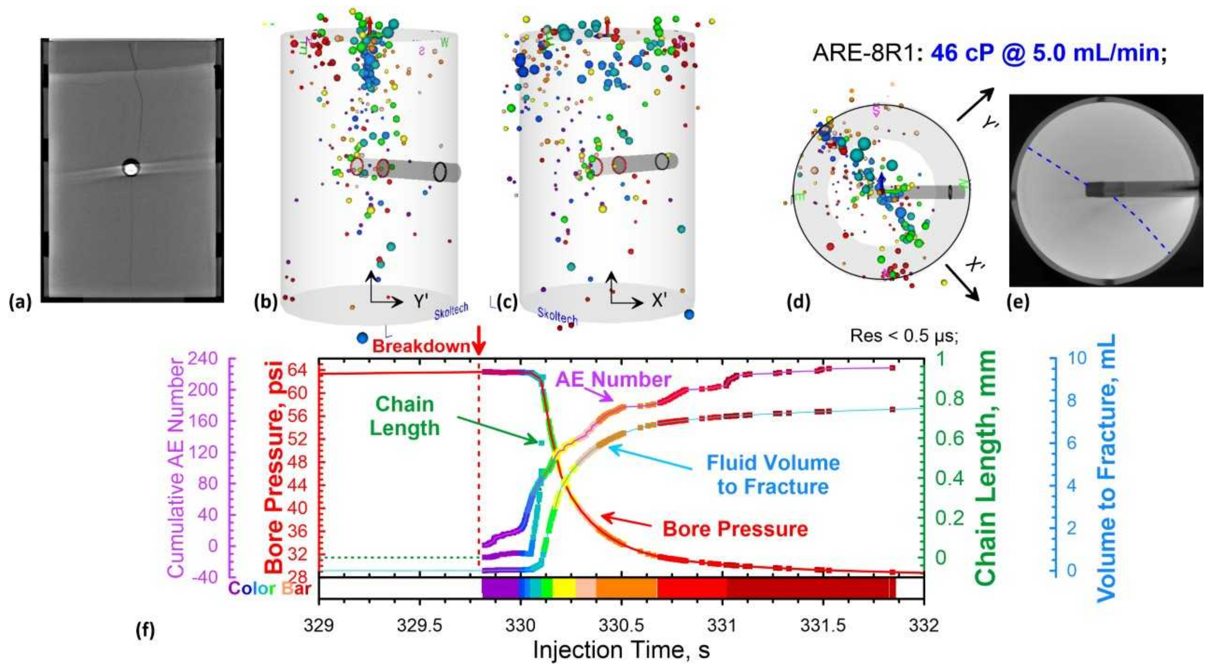
| Sample Number | ARE-1R1 | ARE-1R2 | ARE-2R6 | ARE-3R1 | ARE-4R4 | ARE-8R1 | |
|---|---|---|---|---|---|---|---|
| Sampling depth | m | 5781.28 | 5780.18 | 5787.06 | 5847.87 | 5861.1 | 5873.64 |
| Length | mm | 108.78 | 87.35 | 110.10 | 96.51 | 104.02 | 75.76 |
| Diameter | mm | 49.08 | 49.22 | 48.98 | 49.30 | 49.11 | 49.20 |
| Length/Diameter | 2.22 | 1.77 | 2.25 | 1.96 | 2.12 | 1.54 | |
| Weight | g | 560.23 | 447.60 | 538.60 | 508.10 | 532.70 | 387.24 |
| Volume | cm3 | 205.80 | 166.20 | 207.45 | 184.23 | 197.04 | 144.03 |
| Density | g/cm3 | 2.72 | 2.69 | 2.60 | 2.76 | 2.70 | 2.69 |
| Average effective gas permeability | mD | 4.85 | 4.85 | 0.43 | 0.61 | 0.83 | 0.42 |
| Average porosity | % | 1.95 | 1.95 | 3.45 | 1.98 | 2.05 | 2.13 |
| Uniaxial compressive strength (UCS) | MPa | 86.8 | 86.8 | 78.1 | 397.4 | 121.2 | 247.1 |
| Young’s modulus E | GPa | 51.14 | 51.14 | 46.48 | 79.00 | 52.76 | 55.15 |
| Poisson’s ratio ν | 0.25 | 0.25 | 0.22 | 0.17 | 0.13 | 0.10 |
| Sample | ARE-1R1 | ARE-1R2 | ARE-2R6 | ARE-3R1 | ARE-4R4 | ARE-8R1 |
|---|---|---|---|---|---|---|
| PV, m/s | 4574 | 5227 | 4374 | 5922 | 5928 | 5167 |
| PH, m/s | 5008 | 5241 | 4920 | 5572 | 5630 | 4973 |
| AP, % | −9.4 | −0.27 | −12.5 | 5.9 | 5 | 3.7 |
| Sample | ARE-1R1 | ARE-1R2 | ARE-2R6 | ARE-3R1 | ARE-4R4 | ARE-8R1 | MSS-401 |
|---|---|---|---|---|---|---|---|
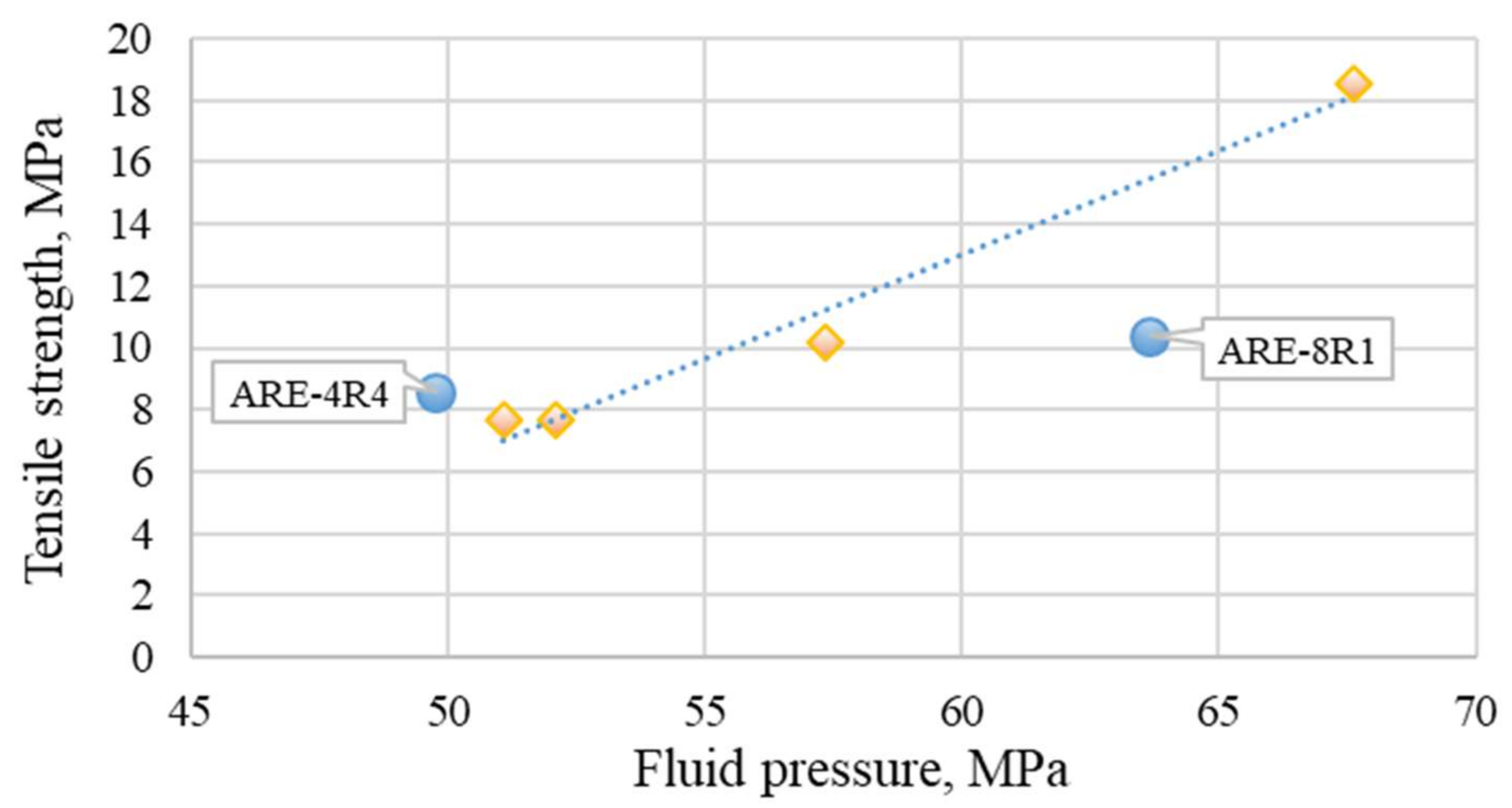
| Tensile strength (TXTR), MPa | 7.65 | 7.65 | 10.20 | 18.55 | 8.60 | 10.40 | − |
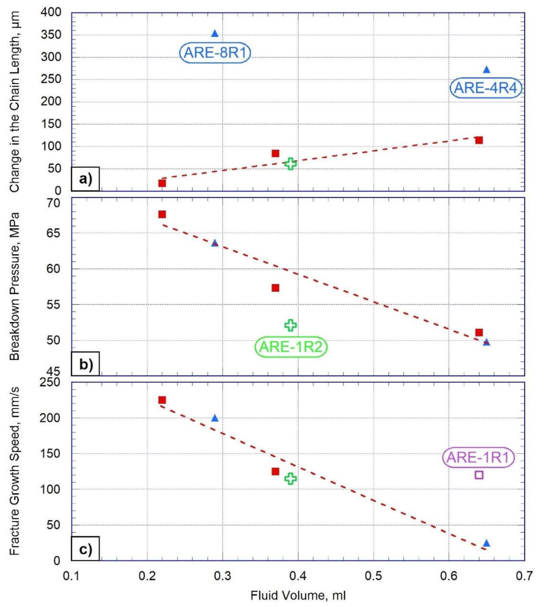
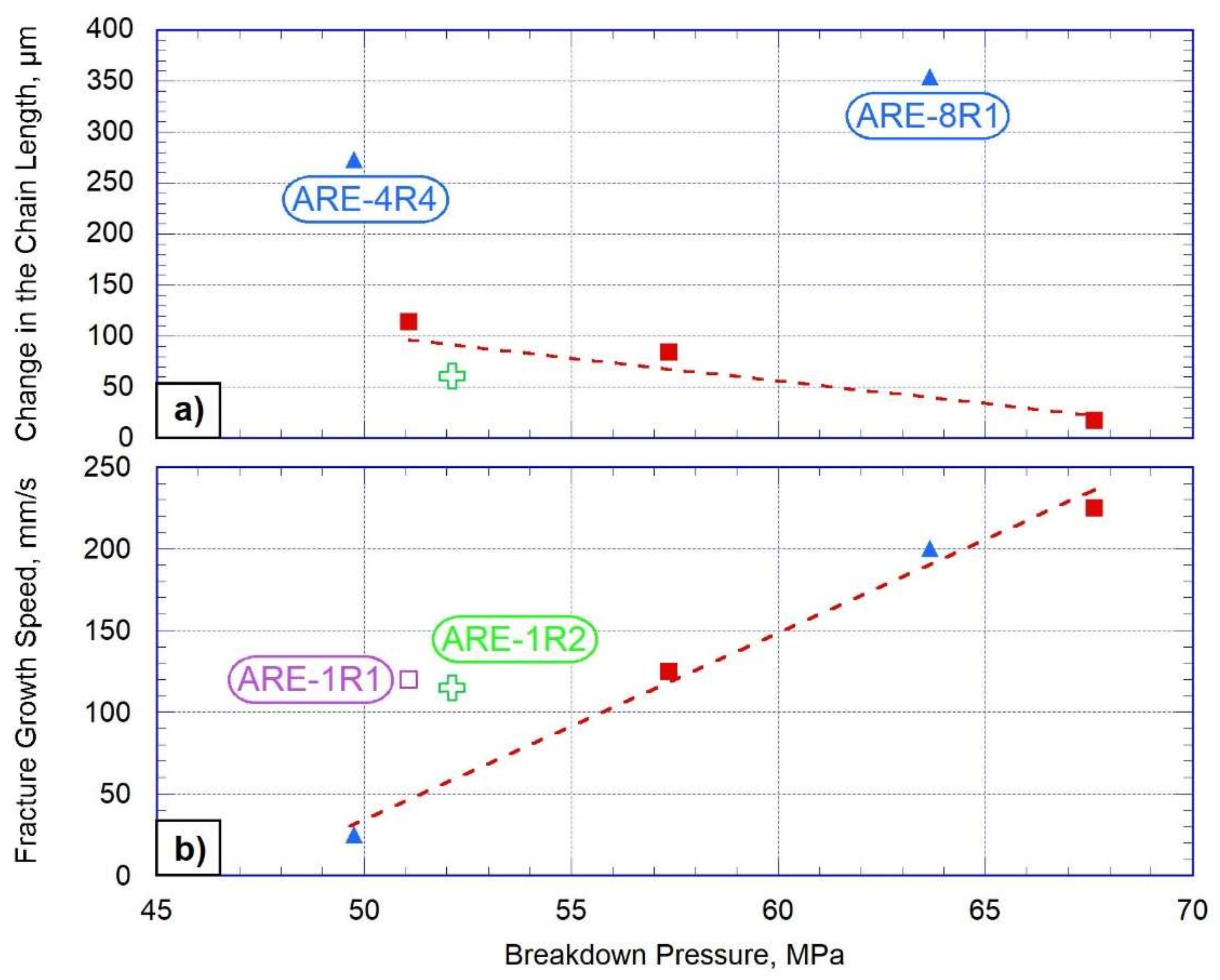
| Breakdown pressure, MPa | 51.08 | 52.12 | 57.35 | 67.63 | 49.76 | 63.66 | 42.50 |
| Change of the chain length at the time of fluid exit, μm | 114 | 61 | 85 | 18 | 273 | 354 | 25 |
| Fluid volume entered into the fracture, mL | 0.64 | 0.39 | 0.37 | 0.22 | 0.65 | 0.29 | 0.11 |
| Fracture propagation speed, mm/s | 120 | 115 | 125 | 225 | 25 | 200 | 0.45–3 |
| Fluid injection rate, mL/min | 5 | 5 | 5 | 5 | 5 | 5 | 0.5 |
| Rate of wellbore pressure drop, MPa/s | −31 | −43 | −91 | −165 | −30 | −192 | −0.61 |
| Fluid viscosity, cP | 46 | 46 | 46 | 46 | 46 | 46 | 100,000 |
| Z coordinate of the wellbore, mm | 73.5 | 55 | 71 | 60 | 70 | 38.5 | 70 |
| Sigma 1, MPa | 54.80 | 54.80 | 54.80 | 54.80 | 54.80 | 54.80 | 16.60 |
| Sigma 3, MPa | 27.38 | 27.38 | 27.38 | 27.38 | 27.38 | 27.38 | 0.27 |
Publisher’s Note: MDPI stays neutral with regard to jurisdictional claims in published maps and institutional affiliations. |
© 2021 by the authors. Licensee MDPI, Basel, Switzerland. This article is an open access article distributed under the terms and conditions of the Creative Commons Attribution (CC BY) license (https://creativecommons.org/licenses/by/4.0/).
Share and Cite
Bobrova, M.; Stanchits, S.; Shevtsova, A.; Filev, E.; Stukachev, V.; Shayahmetov, T. Laboratory Investigation of Hydraulic Fracture Behavior of Unconventional Reservoir Rocks. Geosciences 2021, 11, 292. https://0-doi-org.brum.beds.ac.uk/10.3390/geosciences11070292
Bobrova M, Stanchits S, Shevtsova A, Filev E, Stukachev V, Shayahmetov T. Laboratory Investigation of Hydraulic Fracture Behavior of Unconventional Reservoir Rocks. Geosciences. 2021; 11(7):292. https://0-doi-org.brum.beds.ac.uk/10.3390/geosciences11070292
Chicago/Turabian StyleBobrova, Maria, Sergey Stanchits, Anna Shevtsova, Egor Filev, Vladimir Stukachev, and Tagir Shayahmetov. 2021. "Laboratory Investigation of Hydraulic Fracture Behavior of Unconventional Reservoir Rocks" Geosciences 11, no. 7: 292. https://0-doi-org.brum.beds.ac.uk/10.3390/geosciences11070292