
Fast Directional Changes during Geomagnetic Transitions: Global Reversals or Local Fluctuations?


Abstract
:1. Introduction
2. Methodology
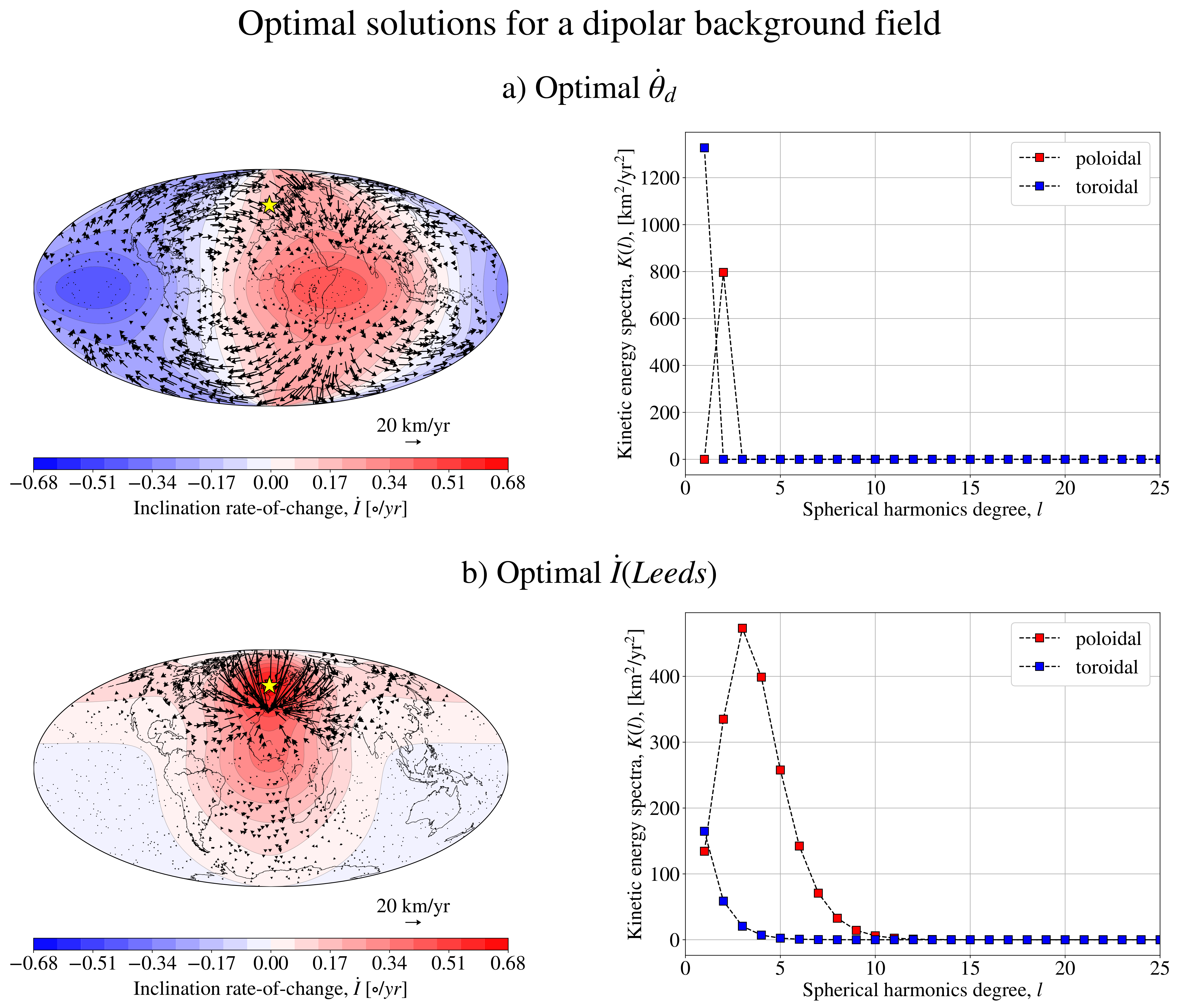
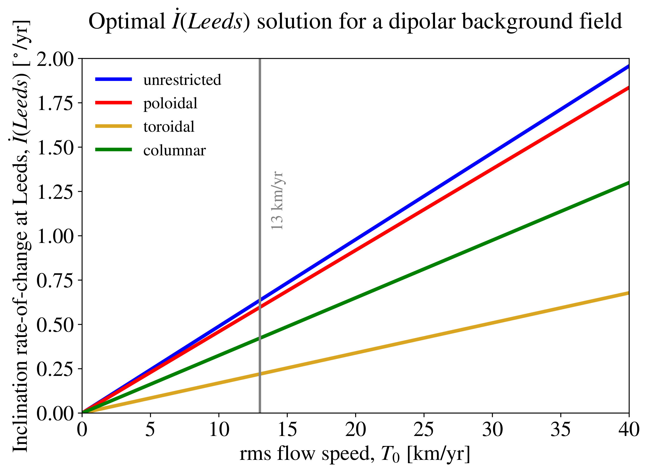
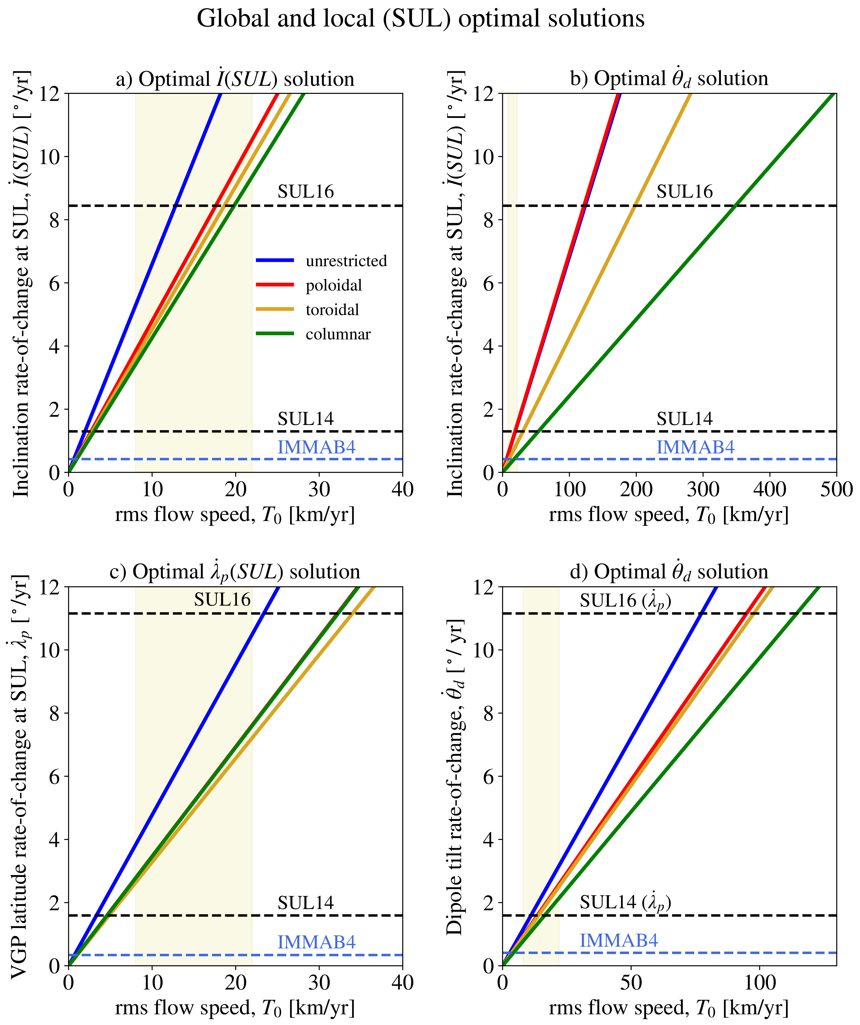
- Unrestricted: no restriction is imposed on the coefficients , and both toroidal and poloidal components are present;
- Poloidal: obtained by setting the toroidal flows to zero, i.e., . A distinguishing feature of purely poloidal flows is the presence of regions of flow downwelling and upwelling, which have been considered as a proxy for enhanced magnetic diffusion [59] and have been connected to the formation of reverse flux patches at the CMB [60], both potentially important features in the interpretation of rapid geomagnetic field variations;
- Toroidal: obtained by setting the poloidal flow to zero, i.e., . A purely toroidal flow allows no upwelling/downwelling since . The physical motivation for a purely toroidal flow derives from the widespread agreement among core flow inversion studies that the toroidal kinetic energy dominates the poloidal kinetic energy at the CMB (see for example [61]). This observation has been considered to confirm the presence of a stratified layer at the top of the outer core [62]. Note however that various studies (e.g., [63,64,65]) suggested that a small poloidal component is necessary to explain the observed SV;
- Columnar: obtained by constraining the flows at the CMB to be the surface expression of columnar flows in the interior of the core and obtained by setting to zero the poloidal coefficients for which is odd and the toroidal coefficients for which is even [66,67]. This representation, encoding equatorial symmetry, is motivated by the evidence for a quasigeostrophic force balance within the outer core [68,69]. The significance of the columnar flows’ approximation to the present study lies in its expected validity over interannual to decadal timescales [68,70]. The columnar flows’ approximation can therefore be considered appropriate for subcentennial field variations, such us the ones presented in SUL14, SUL16, and [16].
Geomagnetic Directional Quantities
3. Pedagogical Examples
3.1. Global vs. Local Quantities
3.2. Influence of Flow Geometry
4. Comparison with Geodynamo Results
4.1. Extreme Directional Changes
4.2. Influence of Truncation
5. Paleomagnetic Calculations
6. Discussion
7. Conclusions
Author Contributions
Funding
Institutional Review Board Statement
Informed Consent Statement
Data Availability Statement
Conflicts of Interest
Abbreviations
| CMB | core-mantle boundary |
| M-B | Matuyama-Brunhes |
| SUL | Sulmona |
| SV | secular variation |
Appendix A. Comparison with the Green Functions Formalism
Appendix B. Analytical Calculation of Simple Optimal Solutions
Appendix B.1. Optimisation of

Appendix B.2. Optimisation of
Appendix B.3. Optimisation of
Appendix C. Maximal Variations for Different Flow Geometries


| Flow Geometry/Model | |||
|---|---|---|---|
| Unrestricted | 1.87 | 8.57 | 6.21 |
| Poloidal | 1.53 | 6.23 | 4.51 |
| Toroidal | 1.40 | 5.88 | 4.27 |
| Columnar | 1.27 | 5.54 | 4.50 |
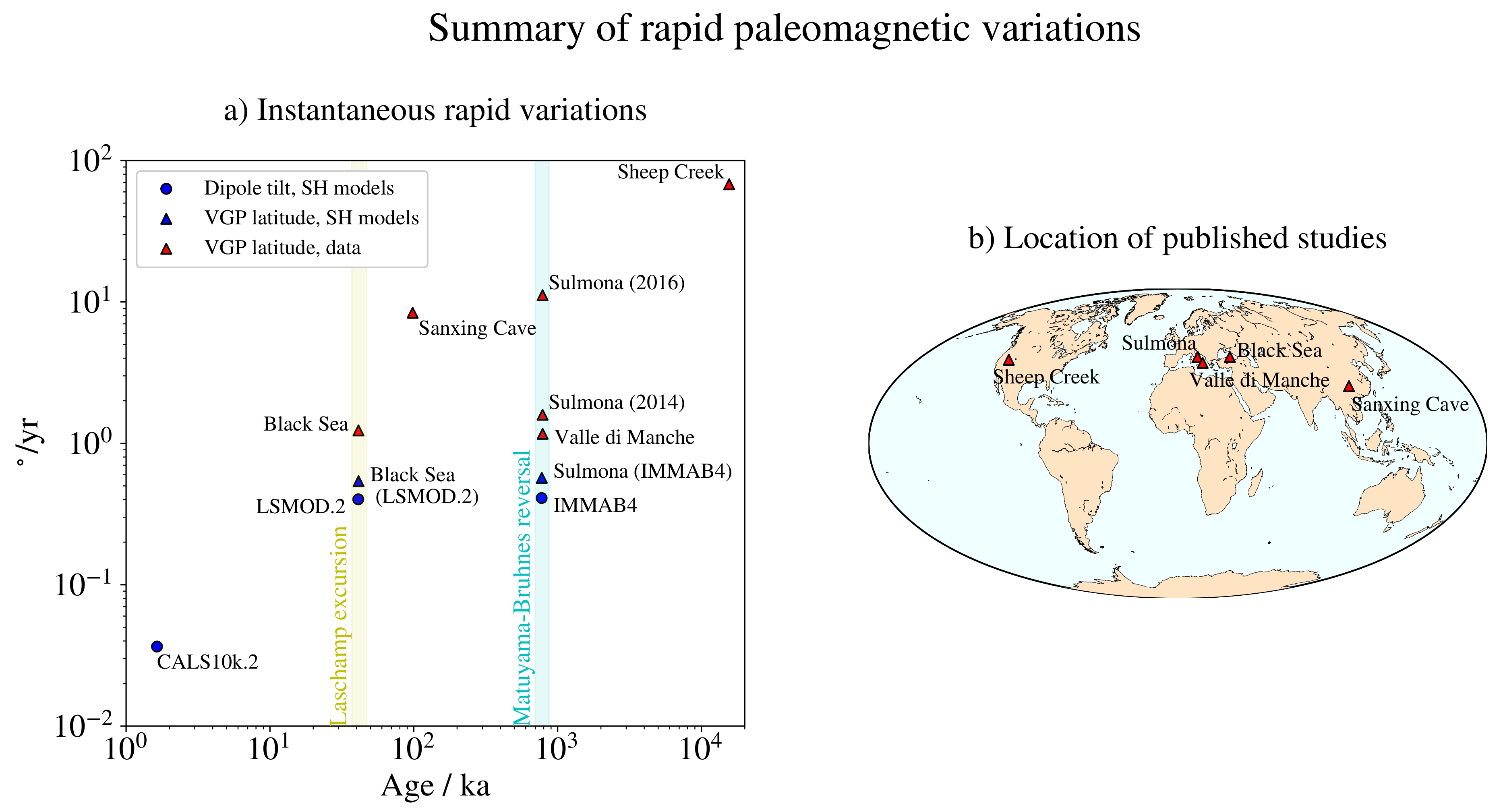
| SUL14 | - | 1.30 | 1.65 |
| SUL16 | - | 8.44 | 11.16 |
| IMMAB4, M-B avg | 0.074 | 0.039 | 0.054 |
| IMMAB4, max | 0.41 | 0.43 | 0.57 |
References
- Gauss, C.F. Allgemeine theorie des erdmagnetismus. In Werke; Springer: Berlin/Heidelberg, Germany, 1877; pp. 119–193. [Google Scholar]
- Gubbins, D.; Jones, A.L.; Finlay, C.C. Fall in Earth’s magnetic field is erratic. Science 2006, 312, 900–902. [Google Scholar] [CrossRef] [PubMed]
- Jackson, A.; Jonkers, A.R.; Walker, M.R. Four centuries of geomagnetic secular variation from historical records. Philos. Trans. R. Soc. Lond. Ser. Math. Phys. Eng. Sci. 2000, 358, 957–990. [Google Scholar] [CrossRef]
- Usui, Y.; Tarduno, J.A.; Watkeys, M.; Hofmann, A.; Cottrell, R.D. Evidence for a 3.45-billion-year-old magnetic remanence: Hints of an ancient geodynamo from conglomerates of South Africa. Geochem. Geophys. Geosyst. 2009, 10, Q09Z07. [Google Scholar] [CrossRef]
- Tarduno, J.A.; Cottrell, R.D.; Watkeys, M.K.; Hofmann, A.; Doubrovine, P.V.; Mamajek, E.E.; Liu, D.; Sibeck, D.G.; Neukirch, L.P.; Usui, Y. Geodynamo, solar wind, and magnetopause 3.4 to 3.45 billion years ago. Science 2010, 327, 1238–1240. [Google Scholar] [CrossRef] [Green Version]
- Tang, F.; Taylor, R.J.; Einsle, J.F.; Borlina, C.S.; Fu, R.R.; Weiss, B.P.; Williams, H.M.; Williams, W.; Nagy, L.; Midgley, P.A.; et al. Secondary magnetite in ancient zircon precludes analysis of a Hadean geodynamo. Proc. Natl. Acad. Sci. USA 2019, 116, 407–412. [Google Scholar] [CrossRef] [PubMed] [Green Version]
- Tarduno, J.A.; Cottrell, R.D.; Bono, R.K.; Oda, H.; Davis, W.J.; Fayek, M.; van’t Erve, O.; Nimmo, F.; Huang, W.; Thern, E.R.; et al. Paleomagnetism indicates that primary magnetite in zircon records a strong Hadean geodynamo. Proc. Natl. Acad. Sci. USA 2020, 117, 2309–2318. [Google Scholar] [CrossRef] [PubMed] [Green Version]
- Johnson, C.; McFadden, P. 5.11.—Time-Averaged Field and Paleosecular Variation. In Treatise on Geophysics, 2nd ed.; Schubert, G., Ed.; Elsevier: Oxford, UK, 2015; pp. 385–417. [Google Scholar] [CrossRef]
- Tauxe, L.; Yamazaki, T. 5.13—Paleointensities. In Treatise on Geophysics, 2nd ed.; Schubert, G., Ed.; Elsevier: Oxford, UK, 2015; pp. 461–509. [Google Scholar] [CrossRef]
- Bogue, S.W.; Glen, J.M. Very rapid geomagnetic field change recorded by the partial remagnetization of a lava flow. Geophys. Res. Lett. 2010, 37, L21308. [Google Scholar] [CrossRef] [Green Version]
- Constable, C.; Korte, M.; Panovska, S. Persistent high paleosecular variation activity in southern hemisphere for at least 10,000 years. Earth Planet. Sci. Lett. 2016, 453, 78–86. [Google Scholar] [CrossRef] [Green Version]
- Okada, M.; Niitsuma, N. Detailed paleomagnetic records during the Brunhes-Matuyama geomagnetic reversal, and a direct determination of depth lag for magnetization in marine sediments. Phys. Earth Planet. Inter. 1989, 56, 133–150. [Google Scholar] [CrossRef]
- Sagnotti, L.; Scardia, G.; Giaccio, B.; Liddicoat, J.C.; Nomade, S.; Renne, P.R.; Sprain, C.J. Extremely rapid directional change during Matuyama-Brunhes geomagnetic polarity reversal. Geophys. J. Int. 2014, 199, 1110–1124. [Google Scholar] [CrossRef]
- Sagnotti, L.; Giaccio, B.; Liddicoat, J.C.; Nomade, S.; Renne, P.R.; Scardia, G.; Sprain, C.J. How fast was the Matuyama-Brunhes geomagnetic reversal? A new subcentennial record from the Sulmona Basin, Central Italy. Geophys. J. Int. 2016, 204, 798–812. [Google Scholar] [CrossRef] [Green Version]
- Okada, M.; Suganuma, Y.; Haneda, Y.; Kazaoka, O. Paleomagnetic direction and paleointensity variations during the Matuyama-Brunhes polarity transition from a marine succession in the Chiba composite section of the Boso Peninsula, central Japan. Earth Planets Space 2017, 69, 45. [Google Scholar] [CrossRef] [Green Version]
- Macrì, P.; Capraro, L.; Ferretti, P.; Scarponi, D. A high-resolution record of the Matuyama-Brunhes transition from the Mediterranean region: The Valle di Manche section (Calabria, Southern Italy). Phys. Earth Planet. Inter. 2018, 278, 1–15. [Google Scholar] [CrossRef]
- Chou, Y.M.; Jiang, X.; Liu, Q.; Hu, H.M.; Wu, C.C.; Liu, J.; Jiang, Z.; Lee, T.Q.; Wang, C.C.; Song, Y.F.; et al. Multidecadally resolved polarity oscillations during a geomagnetic excursion. Proc. Natl. Acad. Sci. USA 2018, 115, 8913–8918. [Google Scholar] [CrossRef] [PubMed] [Green Version]
- Nowaczyk, N.; Arz, H.; Frank, U.; Kind, J.; Plessen, B. Dynamics of the Laschamp geomagnetic excursion from Black Sea sediments. Earth Planet. Sci. Lett. 2012, 351, 54–69. [Google Scholar] [CrossRef]
- Nowaczyk, N.; Frank, U.; Kind, J.; Arz, H. A high-resolution paleointensity stack of the past 14 to 68 ka from Black Sea sediments. Earth Planet. Sci. Lett. 2013, 384, 1–16. [Google Scholar] [CrossRef]
- Liu, J.; Nowaczyk, N.R.; Panovska, S.; Korte, M.; Arz, H.W. The Norwegian-Greenland Sea, the Laschamps, and the Mono Lake Excursions Recorded in a Black Sea Sedimentary Sequence Spanning From 68.9 to 14.5 ka. JGR Solid Earth 2020, 125, e2019JB019225. [Google Scholar] [CrossRef]
- Leonhardt, R.; Fabian, K. Paleomagnetic reconstruction of the global geomagnetic field evolution during the Matuyama/Brunhes transition: Iterative Bayesian inversion and independent verification. Earth Planet. Sci. Lett. 2007, 253, 172–195. [Google Scholar] [CrossRef]
- Korte, M.; Brown, M.C.; Panovska, S.; Wardinski, I. Robust characteristics of the laschamp and mono lake geomagnetic excursions: Results from global field models. Front. Earth Sci. 2019, 7, 86. [Google Scholar] [CrossRef] [Green Version]
- Evans, M.; Muxworthy, A. A re-appraisal of the proposed rapid Matuyama-Brunhes geomagnetic reversal in the Sulmona Basin, Italy. Geophys. J. Int. 2018, 213, 1744–1750. [Google Scholar] [CrossRef] [Green Version]
- Sagnotti, L.; Giaccio, B.; Liddicoat, J.C.; Caricchi, C.; Nomade, S.; Renne, P.R. On the reliability of the Matuyama-Brunhes record in the Sulmona Basin—Comment to ‘A reappraisal of the proposed rapid Matuyama-Brunhes geomagnetic reversal in the Sulmona Basin, Italy’ by Evans and Muxworthy (2018). Geophys. J. Int. 2019, 216, 296–301. [Google Scholar] [CrossRef]
- Finlay, C.C.; Olsen, N.; Kotsiaros, S.; Gillet, N.; Tøffner-Clausen, L. Recent geomagnetic secular variation from Swarm and ground observatories as estimated in the CHAOS-6 geomagnetic field model. Earth Planets Space 2016, 68, 112. [Google Scholar] [CrossRef] [Green Version]
- Davies, C.J.; Constable, C.G. Rapid geomagnetic changes inferred from Earth observations and numerical simulations. Nat. Commun. 2020, 11, 3371. [Google Scholar] [CrossRef] [PubMed]
- Aubert, J.; Labrosse, S.; Poitou, C. Modelling the palaeo-evolution of the geodynamo. Geophys. J. Int. 2009, 179, 1414–1428. [Google Scholar] [CrossRef] [Green Version]
- Glatzmaier, G.A. Geodynamo simulations—How realistic are they? Annu. Rev. Earth Planet. Sci. 2002, 30, 237–257. [Google Scholar] [CrossRef] [Green Version]
- Christensen, U.; Wicht, J. 8.10—Numerical Dynamo Simulations. In Treatise on Geophysics, 2nd ed.; Schubert, G., Ed.; Elsevier: Oxford, UK, 2015; pp. 245–277. [Google Scholar] [CrossRef]
- Sprain, C.J.; Biggin, A.J.; Davies, C.J.; Bono, R.K.; Meduri, D.G. An assessment of long duration geodynamo simulations using new paleomagnetic modeling criteria (QPM). Earth Planet. Sci. Lett. 2019, 526, 115758. [Google Scholar] [CrossRef]
- Meduri, D.G.; Biggin, A.J.; Davies, C.J.; Bono, R.K.; Sprain, C.J.; Wicht, J. Numerical Dynamo Simulations Reproduce Paleomagnetic Field Behavior. Geophys. Res. Lett. 2021, 48, e2020GL090544. [Google Scholar] [CrossRef]
- Glatzmaier, G.A.; Coe, R.S.; Hongre, L.; Roberts, P.H. The role of the Earth’s mantle in controlling the frequency of geomagnetic reversals. Nature 1999, 401, 885–890. [Google Scholar] [CrossRef]
- Kutzner, C.; Christensen, U.R. Simulated geomagnetic reversals and preferred virtual geomagnetic pole paths. Geophys. J. Int. 2004, 157, 1105–1118. [Google Scholar] [CrossRef] [Green Version]
- Olson, P.L.; Glatzmaier, G.A.; Coe, R.S. Complex polarity reversals in a geodynamo model. Earth Planet. Sci. Lett. 2011, 304, 168–179. [Google Scholar] [CrossRef]
- Shao, J.C.; Fuller, M.; Tanimoto, T.; Dunn, J.R.; Stone, D.B. Spherical harmonic analyses of paleomagnetic data: The time-averaged geomagnetic field for the past 5 Myr and the Brunhes-Matuyama reversal. J. Geophys. Res. Solid Earth 1999, 104, 5015–5030. [Google Scholar] [CrossRef] [Green Version]
- Ingham, M.; Turner, G. Behaviour of the geomagnetic field during the Matuyama-Brunhes polarity transition. Phys. Earth Planet. Inter. 2008, 168, 163–178. [Google Scholar] [CrossRef]
- Valet, J.P.; Fournier, A. Deciphering records of geomagnetic reversals. Rev. Geophys. 2016, 54, 410–446. [Google Scholar] [CrossRef]
- Singer, B.S.; Jicha, B.R.; Mochizuki, N.; Coe, R.S. Synchronizing volcanic, sedimentary, and ice core records of Earth’s last magnetic polarity reversal. Sci. Adv. 2019, 5, eaaw4621. [Google Scholar] [CrossRef] [PubMed] [Green Version]
- Just, J.; Sagnotti, L.; Nowaczyk, N.R.; Francke, A.; Wagner, B. Recordings of Fast Paleomagnetic Reversals in a 1.2 Ma Greigite-Rich Sediment Archive From Lake Ohrid, Balkans. J. Geophys. Res. Solid Earth 2019, 124, 12445–12464. [Google Scholar] [CrossRef]
- Backus, G.; Bullard, E.C. Kinematics of geomagnetic secular variation in a perfectly conducting core. Philos. Trans. R. Soc. Lond. Ser. A Math. Phys. Sci. 1968, 263, 239–266. [Google Scholar] [CrossRef]
- Jackson, A. Time-dependency of tangentially geostrophic core surface motions. Phys. Earth Planet. Inter. 1997, 103, 293–311. [Google Scholar] [CrossRef]
- Amit, H.; Olson, P. Time-average and time-dependent parts of core flow. Phys. Earth Planet. Inter. 2006, 155, 120–139. [Google Scholar] [CrossRef]
- Finlay, C.C.; Amit, H. On flow magnitude and field-flow alignment at Earth’s core surface. Geophys. J. Int. 2011, 186, 175–192. [Google Scholar] [CrossRef] [Green Version]
- Driscoll, P.; Olson, P. Effects of buoyancy and rotation on the polarity reversal frequency of gravitationally driven numerical dynamos. Geophys. J. Int. 2009, 178, 1337–1350. [Google Scholar] [CrossRef] [Green Version]
- Olson, P.; Driscoll, P.; Amit, H. Dipole collapse and reversal precursors in a numerical dynamo. Phys. Earth Planet. Inter. 2009, 173, 121–140. [Google Scholar] [CrossRef]
- Wicht, J.; Olson, P. A detailed study of the polarity reversal mechanism in a numerical dynamo model. Geochem. Geophys. Geosystems 2004, 5. [Google Scholar] [CrossRef] [Green Version]
- Olson, P. Gravitational dynamos and the low-frequency geomagnetic secular variation. Proc. Natl. Acad. Sci. USA 2007, 104, 20159–20166. [Google Scholar] [CrossRef] [PubMed] [Green Version]
- Livermore, P.W.; Fournier, A.; Gallet, Y. Core-flow constraints on extreme archeomagnetic intensity changes. Earth Planet. Sci. Lett. 2014, 387, 145–156. [Google Scholar] [CrossRef] [Green Version]
- Ben-Yosef, E.; Tauxe, L.; Levy, T.E.; Shaar, R.; Ron, H.; Najjar, M. Geomagnetic intensity spike recorded in high resolution slag deposit in Southern Jordan. Earth Planet. Sci. Lett. 2009, 287, 529–539. [Google Scholar] [CrossRef]
- Shaar, R.; Ben-Yosef, E.; Ron, H.; Tauxe, L.; Agnon, A.; Kessel, R. Geomagnetic field intensity: How high can it get? How fast can it change? Constraints from Iron Age copper slag. Earth Planet. Sci. Lett. 2011, 301, 297–306. [Google Scholar] [CrossRef]
- Shaar, R.; Tauxe, L.; Ron, H.; Ebert, Y.; Zuckerman, S.; Finkelstein, I.; Agnon, A. Large geomagnetic field anomalies revealed in Bronze to Iron Age archeomagnetic data from Tel Megiddo and Tel Hazor, Israel. Earth Planet. Sci. Lett. 2016, 442, 173–185. [Google Scholar] [CrossRef] [Green Version]
- Ben-Yosef, E.; Millman, M.; Shaar, R.; Tauxe, L.; Lipschits, O. Six centuries of geomagnetic intensity variations recorded by royal Judean stamped jar handles. Proc. Natl. Acad. Sci. USA 2017, 114, 2160–2165. [Google Scholar] [CrossRef] [PubMed] [Green Version]
- Livermore, P.W.; Gallet, Y.; Fournier, A. Archeomagnetic intensity variations during the era of geomagnetic spikes in the Levant. Phys. Earth Planet. Inter. 2021, 312, 106657. [Google Scholar] [CrossRef]
- Holme, R. 8.04—Large-Scale Flow in the Core. In Treatise on Geophysics, 2nd ed.; Schubert, G., Ed.; Elsevier: Oxford, UK, 2015; pp. 91–113. [Google Scholar] [CrossRef]
- Tauxe, L.; Banerjee, S.; Butler, R.; Van der Voo, R. Essentials of Paleomagnetism, 5th ed.; University of California Press: Oakland, CA, USA, 2018. [Google Scholar]
- Engdahl, E.R.; Johnson, L.E. Differential PcP Travel Times and the Radius of the Core. Geophys. J. Int. 1974, 39, 435–456. [Google Scholar] [CrossRef] [Green Version]
- Tilgner, A. 8.07—Rotational Dynamics of the Core. In Treatise on Geophysics, 2nd ed.; Schubert, G., Ed.; Elsevier: Oxford, UK, 2015; pp. 183–212. [Google Scholar] [CrossRef]
- Roberts, P.; Scott, S. On analysis of the secular variation. J. Geomagn. Geoelectr. 1965, 17, 137–151. [Google Scholar] [CrossRef]
- Amit, H.; Christensen, U.R. Accounting for magnetic diffusion in core flow inversions from geomagnetic secular variation. Geophys. J. Int. 2008, 175, 913–924. [Google Scholar] [CrossRef] [Green Version]
- Terra-Nova, F.; Amit, H.; Hartmann, G.A.; Trindade, R.I. Using archaeomagnetic field models to constrain the physics of the core: Robustness and preferred locations of reversed flux patches. Geophys. J. Int. 2016, 206, 1890–1913. [Google Scholar] [CrossRef] [Green Version]
- Baerenzung, J.; Holschneider, M.; Lesur, V. The flow at the Earth’s core-mantle boundary under weak prior constraints. J. Geophys. Res. Solid Earth 2016, 121, 1343–1364. [Google Scholar] [CrossRef] [Green Version]
- Whaler, K. Does the whole of the Earth’s core convect? Nature 1980, 287, 528–530. [Google Scholar] [CrossRef]
- Whaler, K. Geomagnetic evidence for fluid upwelling at the core-mantle boundary. Geophys. J. Int. 1986, 86, 563–588. [Google Scholar] [CrossRef]
- Amit, H. Can downwelling at the top of the Earth’s core be detected in the geomagnetic secular variation? Phys. Earth Planet. Inter. 2014, 229, 110–121. [Google Scholar] [CrossRef]
- Lesur, V.; Whaler, K.; Wardinski, I. Are geomagnetic data consistent with stably stratified flow at the core-mantle boundary? Geophys. J. Int. 2015, 201, 929–946. [Google Scholar] [CrossRef]
- Pais, M.; Jault, D. Quasi-geostrophic flows responsible for the secular variation of the Earth’s magnetic field. Geophys. J. Int. 2008, 173, 421–443. [Google Scholar] [CrossRef] [Green Version]
- Amit, H.; Pais, M.A. Differences between tangential geostrophy and columnar flow. Geophys. J. Int. 2013, 194, 145–157. [Google Scholar] [CrossRef] [Green Version]
- Gillet, N.; Schaeffer, N.; Jault, D. Rationale and geophysical evidence for quasi-geostrophic rapid dynamics within the Earth’s outer core. Phys. Earth Planet. Inter. 2011, 187, 380–390. [Google Scholar] [CrossRef] [Green Version]
- Aubert, J.; Gastine, T.; Fournier, A. Spherical convective dynamos in the rapidly rotating asymptotic regime. J. Fluid Mech. 2017, 813, 558–593. [Google Scholar] [CrossRef] [Green Version]
- Jault, D. Axial invariance of rapidly varying diffusionless motions in the Earth’s core interior. Phys. Earth Planet. Inter. 2008, 166, 67–76. [Google Scholar] [CrossRef] [Green Version]
- Gubbins, D.; Roberts, N. Use of the frozen flux approximation in the interpretation of archaeomagnetic and palaeomagnetic data. Geophys. J. Int. 1983, 73, 675–687. [Google Scholar] [CrossRef] [Green Version]
- Johnson, C.L.; Constable, C.G. The time-averaged geomagnetic field: Global and regional biases for 0–5 Ma. Geophys. J. Int. 1997, 131, 643–666. [Google Scholar] [CrossRef] [Green Version]
- Gubbins, D.; Herrero-Bervera, E. Encyclopedia of Geomagnetism and Paleomagnetism; Springer Science & Business Media: Dordrecht, The Netherlands, 2007. [Google Scholar]
- Finlay, C.C.; Kloss, C.; Olsen, N.; Hammer, M.D.; Tøffner-Clausen, L.; Grayver, A.; Kuvshinov, A. The CHAOS-7 geomagnetic field model and observed changes in the South Atlantic Anomaly. Earth Planets Space 2020, 72, 1–31. [Google Scholar] [CrossRef]
- Gillet, N.; Pais, M.; Jault, D. Ensemble inversion of time-dependent core flow models. Geochem. Geophys. Geosyst. 2009, 10, Q06004. [Google Scholar] [CrossRef] [Green Version]
- Baerenzung, J.; Holschneider, M.; Lesur, V. Bayesian inversion for the filtered flow at the Earth’s core-mantle boundary. J. Geophys. Res. Solid Earth 2014, 119, 2695–2720. [Google Scholar] [CrossRef] [Green Version]
- Gillet, N.; Barrois, O.; Finlay, C.C. Stochastic forecasting of the geomagnetic field from the COV-OBS. x1 geomagnetic field model, and candidate models for IGRF-12. Earth Planets Space 2015, 67, 71. [Google Scholar] [CrossRef] [Green Version]
- Barrois, O.; Gillet, N.; Aubert, J. Contributions to the geomagnetic secular variation from a reanalysis of core surface dynamics. Geophys. J. Int. 2017, 211, 50–68. [Google Scholar] [CrossRef]
- Schaeffer, N.; Jault, D.; Nataf, H.C.; Fournier, A. Turbulent geodynamo simulations: A leap towards Earth’s core. Geophys. J. Int. 2017, 211, 1–29. [Google Scholar] [CrossRef] [Green Version]
- Sheyko, A.; Finlay, C.; Favre, J.; Jackson, A. Scale separated low viscosity dynamos and dissipation within the Earth’s core. Sci. Rep. 2018, 8, 1–7. [Google Scholar] [CrossRef]
- Jackson, A.; Finlay, C. 5.05—Geomagnetic Secular Variation and Its Applications to the Core. In Treatise on Geophysics, 2nd ed.; Schubert, G., Ed.; Elsevier: Oxford, UK, 2015; pp. 137–184. [Google Scholar] [CrossRef]
- Brown, M.; Korte, M.; Holme, R.; Wardinski, I.; Gunnarson, S. Earth’s magnetic field is probably not reversing. Proc. Natl. Acad. Sci. USA 2018, 115, 5111–5116. [Google Scholar] [CrossRef] [Green Version]
- Clement, B.M.; Kent, D.V. Geomagnetic Polarity Transition Records from Five Hydraulic Piston Core Sites in the North Atlantic; Initial Reports of the Deep Sea Drilling Project 94; Columbia University Academic Commons: New York, NY, USA, 1987. [Google Scholar]
- McElhinny, M.W.; Lock, J. IAGA paleomagnetic databases with Access. Surv. Geophys. 1996, 17, 575–591. [Google Scholar] [CrossRef]
- Channell, J.; Lehman, B. The last two geomagnetic polarity reversals recorded in high-deposition-rate sediment drifts. Nature 1997, 389, 712–715. [Google Scholar] [CrossRef]
- Clement, B.M. Dependence of the duration of geomagnetic polarity reversals on site latitude. Nature 2004, 428, 637–640. [Google Scholar] [CrossRef] [PubMed]
- Clement, B.M.; Kent, D.V. Latitudinal dependency of geomagnetic polarity transition durations. Nature 1984, 310, 488–491. [Google Scholar] [CrossRef]
- Kadlec, J.; Chadima, M.; Pruner, P.; Schnabl, P. Paleomagnetické datování sedimentů v jeskyni “Za Hájovnou” v Javoříčku-předběžné vỳsledky. Přírodovědné Studie Muzea Prostějovska 2005, 8, 75–82. [Google Scholar]
- Kadlec, J.; Čížková, K.; Šlechta, S. New updated results of paleomagnetic dating of cave deposits exposed in the “Za Hájovnou” Cave, Javoříčko Karst. Acta Musei Natl. Pragae Ser. B Hist. Nat. 2014, 70, 27–34. [Google Scholar] [CrossRef] [Green Version]
- Pares, J.; Perez-Gonzalez, A. Paleomagnetic age for hominid fossils at Atapuerca archaeological site, Spain. Science 1995, 269, 830–832. [Google Scholar] [CrossRef]
- Moreno, D.; Falgueres, C.; Pérez-González, A.; Voinchet, P.; Ghaleb, B.; Despriée, J.; Bahain, J.J.; Sala, R.; Carbonell, E.; de Castro, J.M.B.; et al. New radiometric dates on the lowest stratigraphical section (TD1 to TD6) of Gran Dolina site (Atapuerca, Spain). Quat. Geochronol. 2015, 30, 535–540. [Google Scholar] [CrossRef]
- Parés, J.M.; Álvarez, C.; Sier, M.; Moreno, D.; Duval, M.; Woodhead, J.; Ortega, A.; Campaña, I.; Rosell, J.; de Castro, J.B.; et al. Chronology of the cave interior sediments at Gran Dolina archaeological site, Atapuerca (Spain). Quat. Sci. Rev. 2018, 186, 1–16. [Google Scholar] [CrossRef]
- Panovska, S.; Korte, M.; Constable, C.G. One Hundred Thousand Years of Geomagnetic Field Evolution. Rev. Geophys. 2019, 57, 1289–1337. [Google Scholar] [CrossRef] [Green Version]
- Panovska, S.; Constable, C.G.; Brown, M.C. Global and Regional Assessments of Paleosecular Variation Activity Over the Past 100 ka. Geochem. Geophys. Geosyst. 2018, 19, 1559–1580. [Google Scholar] [CrossRef]
- Bullard, E.C.; Gellman, H. Homogeneous dynamos and terrestrial magnetism. Philos. Trans. R. Soc. London. Ser. A Math. Phys. Sci. 1954, 247, 213–278. [Google Scholar]


Publisher’s Note: MDPI stays neutral with regard to jurisdictional claims in published maps and institutional affiliations. |
© 2021 by the authors. Licensee MDPI, Basel, Switzerland. This article is an open access article distributed under the terms and conditions of the Creative Commons Attribution (CC BY) license (https://creativecommons.org/licenses/by/4.0/).
Share and Cite
Maffei, S.; Livermore, P.W.; Mound, J.E.; Greenwood, S.; Davies, C.J. Fast Directional Changes during Geomagnetic Transitions: Global Reversals or Local Fluctuations? Geosciences 2021, 11, 318. https://0-doi-org.brum.beds.ac.uk/10.3390/geosciences11080318
Maffei S, Livermore PW, Mound JE, Greenwood S, Davies CJ. Fast Directional Changes during Geomagnetic Transitions: Global Reversals or Local Fluctuations? Geosciences. 2021; 11(8):318. https://0-doi-org.brum.beds.ac.uk/10.3390/geosciences11080318
Chicago/Turabian StyleMaffei, Stefano, Philip W. Livermore, Jon E. Mound, Sam Greenwood, and Christopher J. Davies. 2021. "Fast Directional Changes during Geomagnetic Transitions: Global Reversals or Local Fluctuations?" Geosciences 11, no. 8: 318. https://0-doi-org.brum.beds.ac.uk/10.3390/geosciences11080318