
Holocene Sea-Level Changes in Southern Brazil Based on High-Resolution Radar Stratigraphy

 ,
, 
Abstract
:1. Introduction

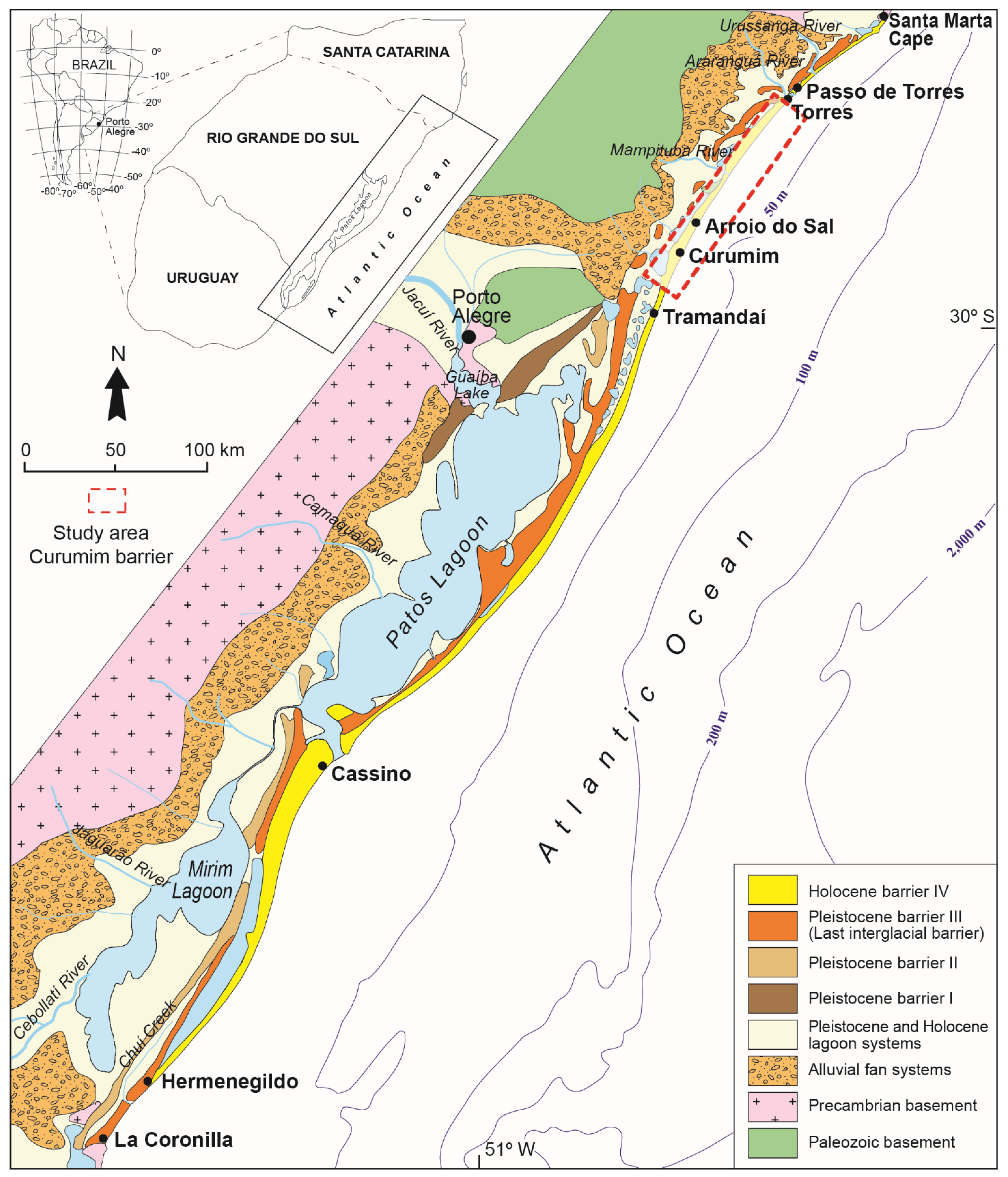
2. Regional Setting
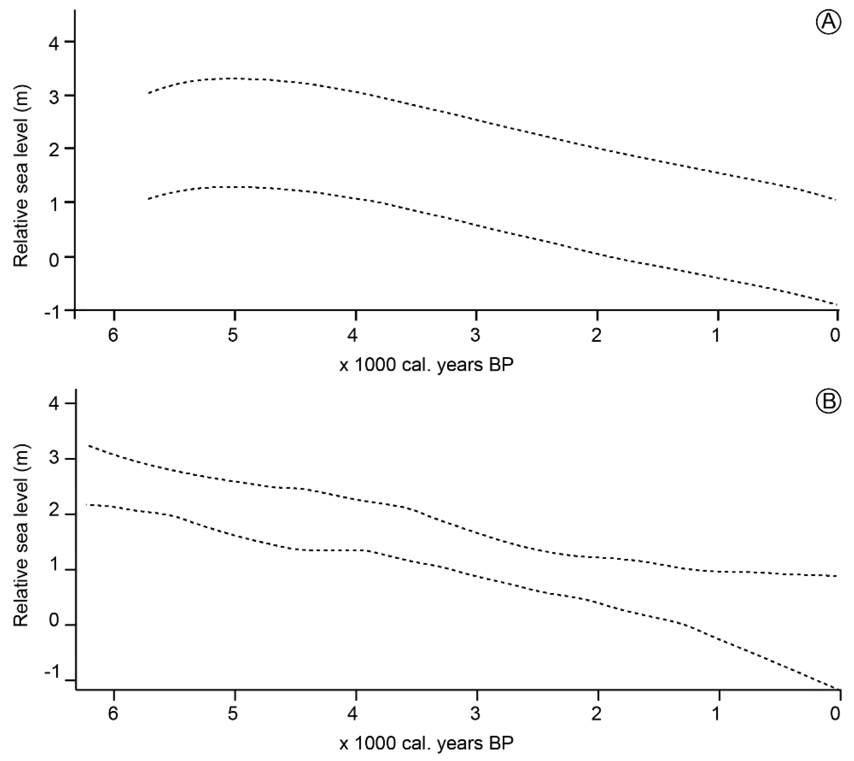
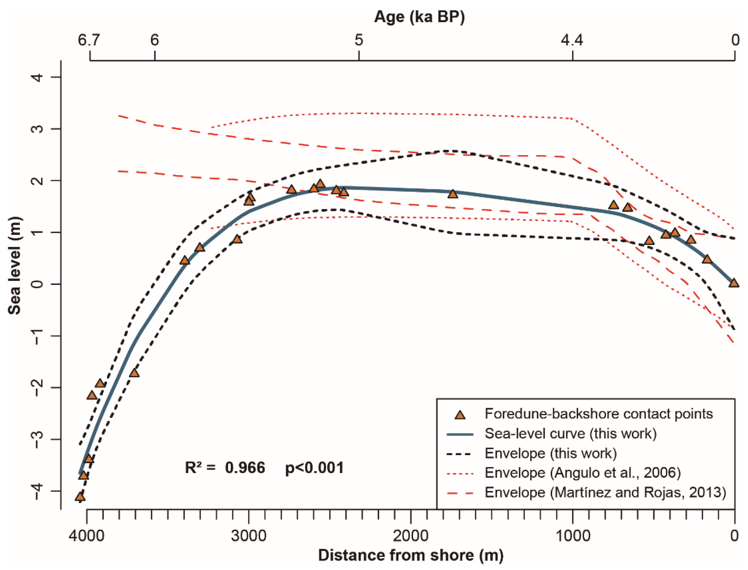
Sea-Level History
3. Materials and Methods
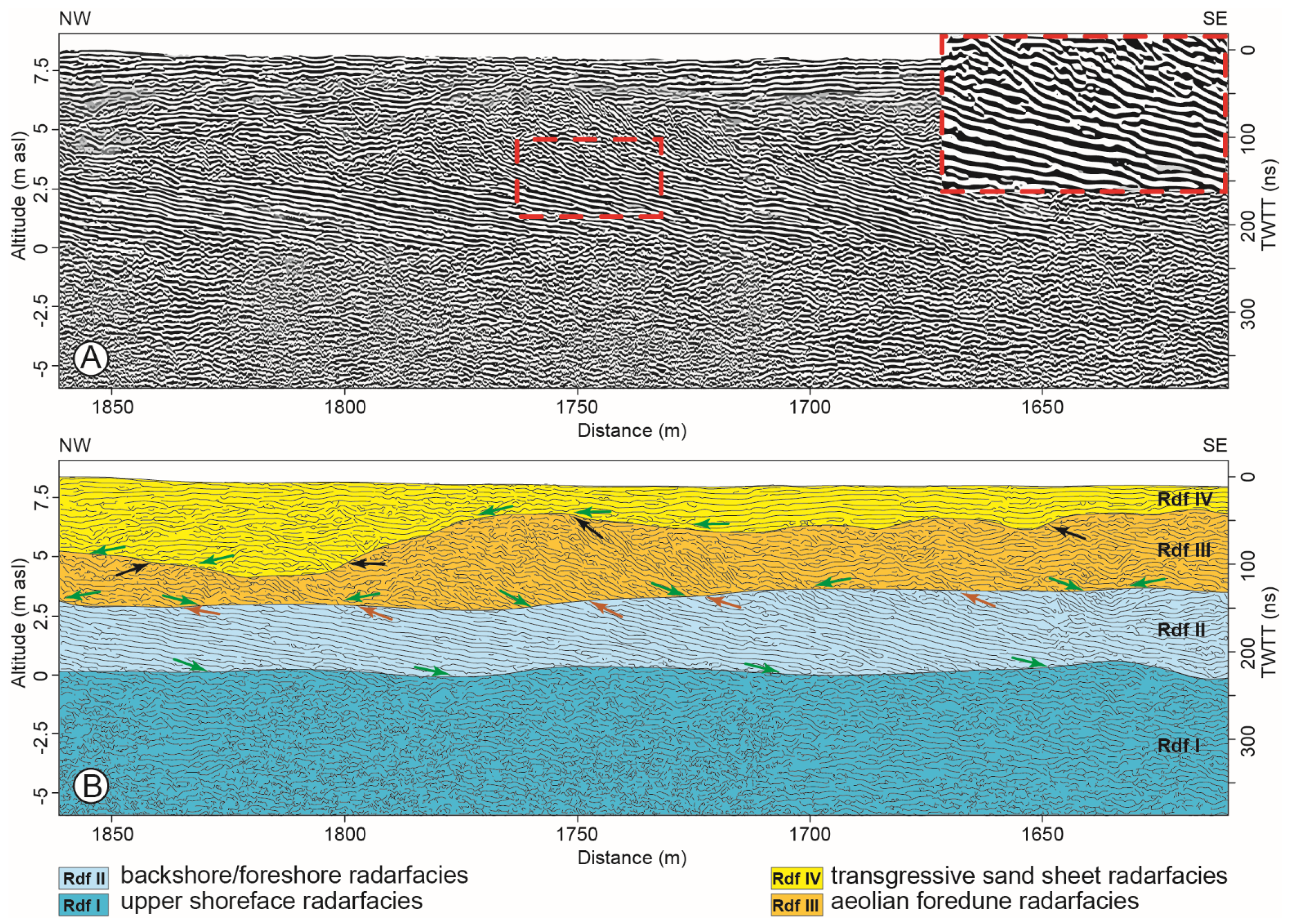
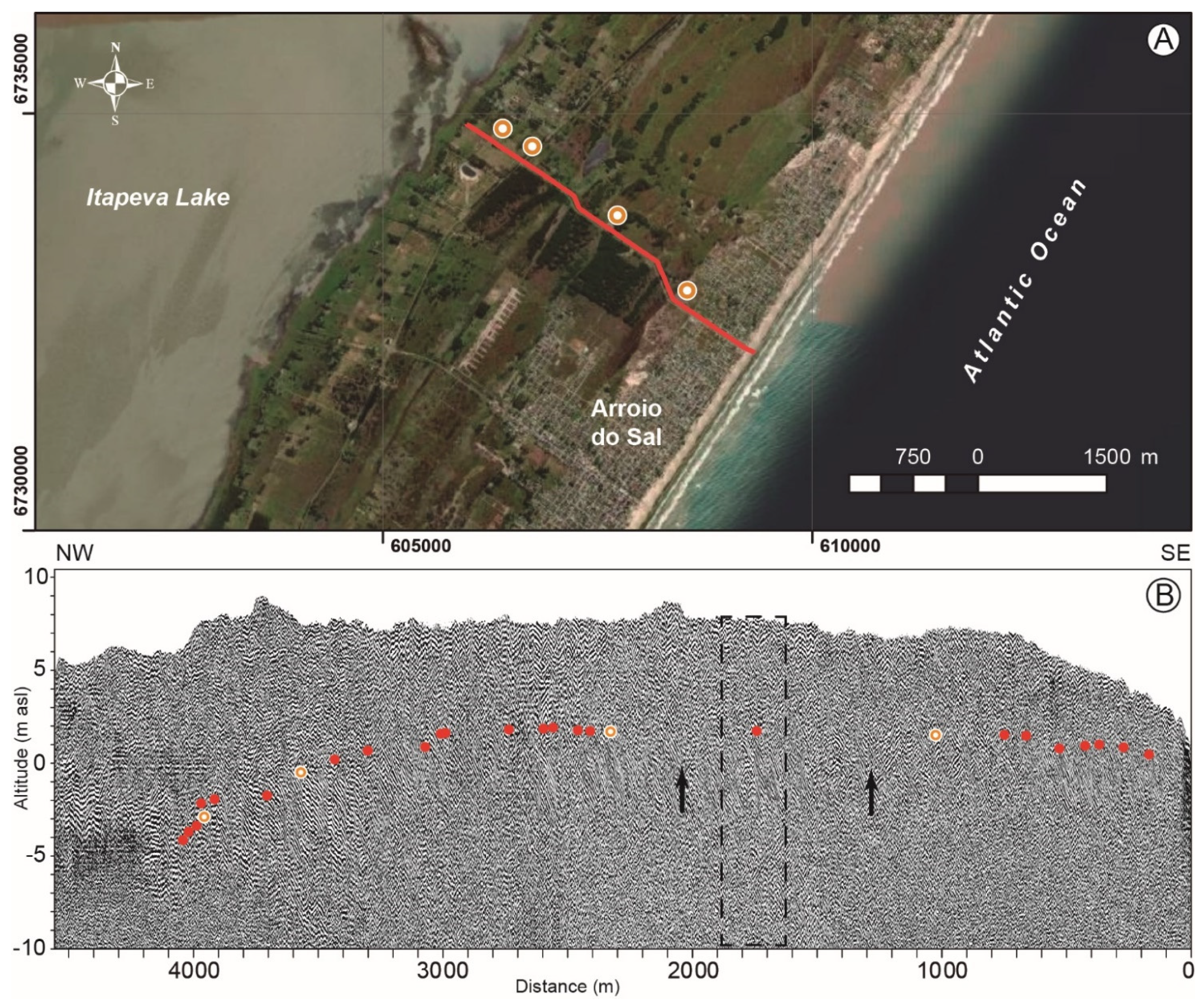
3.1. Ground Penetrating Radar (GPR) Profile
3.2. Global Navigation Satellite System (GNSS) Profile
3.3. OSL Ages
3.4. Geostatistic
4. Results
5. Discussion
6. Conclusions
Supplementary Materials
Author Contributions
Funding
Institutional Review Board Statement
Informed Consent Statement
Data Availability Statement
Acknowledgments
Conflicts of Interest
References
- Martin, L.; Flexor, J.M.; Vilas-Boas, G.S.; Bittencourt, A.C.S.P.; Guimarães, M.M.M. Courbe de variation du niveau relative de la mer au cours des 7000 dernie’res anne’es sur un secteur homoge’ne du littoral bre’ silien (nord de Salvador—Bahia). In Proceedings of the International Symposium on Coastal Evolution in the Quaternary, São Paulo, Brazil, 11–18 September 1978; Suguio, K., Fairchild, T.R., Martin, L., Flexor, J.M., Eds.; USP: São Paulo, Brasil, 1979; pp. 264–295. [Google Scholar]
- Angulo, R.J.; Lessa, G. The Brazilian sea level curves: A critical review with emphasis on the curves from Paranaguá’ and Cananéia regions. Mar. Geol. 1997, 140, 141–166. [Google Scholar] [CrossRef] [Green Version]
- Martin, L.; Dominguez, J.M.L.; Bittencourt, A.C.S.P. Fluctuating Holocene sea levels is eastern and southeastern Brazil: Evidence from a multiple fossil and geometric indicators. J. Coast. Res. 2003, 19, 101–124. [Google Scholar]
- Angulo, R.J.; Lessa, G.C.; Souza, M.C. A critical review of Mid- to Late-Holocene sea-level fluctuations on the eastern Brazilian coastline. Quat. Sci. Rev. 2006, 25, 486–506. [Google Scholar] [CrossRef]
- Tomazelli, L.J.; Villwock, J.A. Processos Erosivos na Costa do Rio Grande do Sul, Brasil: Evidências de uma Provável Tendência Contemporânea de Elevação do Nível Relativo do Mar. In Proceedings of the 2nd Congresso da Associação Brasileira de Estudos do Quaternário, Rio de Janeiro, Brazil, 10–16 July 1989; UFRJ: Rio de Janeiro, Brazil, 1989; p. 16. [Google Scholar]
- Barboza, E.G.; Tomazelli, L.J. Erosional features of the eastern margin of the Patos Lagoon, southern Brazil: Significance for Holocene history. J. Coast. Res. 2003, 35, 260–264. [Google Scholar]
- Dillenburg, S.R.; Tomazelli, L.J.; Hesp, P.A.; Barboza, E.G.; Clerot, L.C.P.; Silva, D.B. Stratigraphy and evolution of a prograded, transgressive dunefield barrier in southern Brazil. J. Coast. Res. 2006, 39, 132–135. [Google Scholar]
- Biancini da Silva, A. Mapeamento e Caracterização dos Depósitos em Subsuperfície do Setor Meridional da Planície Costeira sul de Santa Catarina. Master’s Thesis, PPGGEO/UFRGS, Porto Alegre, Brazil, 2009; 66p. Available online: http://hdl.handle.net/10183/220100 (accessed on 20 May 2021).
- Dillenburg, S.R.; Barboza, E.G.; Rosa, M.L.C.C.; Caron, F.; Sawakuchi, A. The complex prograded Cassino barrier in Southern Brazil: Geological and morphological evolution and records of climatic, oceanographic and sea-level changes in the last 7-6 ka. Mar. Geol. 2017, 390, 106–119. [Google Scholar] [CrossRef]
- van Heteren, S.; Huntley, D.J.; van de Plassche, O.; Lubberts, R.K. Optical dating of dune sand for the study of sea-level change. Geology 2000, 28, 411–414. [Google Scholar] [CrossRef]
- Brooke, B.P.; Huanga, Z.; Nicholas, W.A.; Oliver, T.S.N.; Tamura, T.; Woodroffe, C.D.; Nichol, S.L. Relative sea-level records preserved in Holocene beach-ridge strandplains–An example from tropical northeastern Australia. Mar. Geol. 2019, 411, 107–118. [Google Scholar] [CrossRef]
- Oliver, T.S.N.; Murray-Wallace, C.V.; Woodroffe, C.D. Holocene shoreline progradation and coastal evolution at Guichen and Rivoli Bays, southern Australia. Holocene 2020, 30, 106–124. [Google Scholar] [CrossRef]
- Costas, S.; Ferreira, O.; Plomaritis, T.A.; Leorri, E. Coastal barrier stratigraphy for Holocene high-resolution sea-level reconstruction. Sci. Rep. 2016, 6, 38726. [Google Scholar] [CrossRef] [Green Version]
- Dougherty, A.J. Extracting a record of Holocene storm erosion and deposition preserved in the morphostratigraphy of a prograded coastal barrier. Cont. Shelf Res. 2014, 86, 116–131. [Google Scholar] [CrossRef]
- Dillenburg, S.R.; Barboza, E.G. The Strike-Fed Sandy Coast of Southern Brazil. In Sedimentary Coastal Zones from High to Low Latitudes: Similarities and Differences; Martini, I.P., Wanless, H.R., Eds.; Geological Society: London, UK, 2014; Special Publications 388; pp. 333–352. [Google Scholar] [CrossRef]
- Fernandez, G.B.; Rocha, T.B.; Barboza, E.G.; Dillenburg, S.R.; Rosa, M.L.C.C.; Angulo, R.J.; Souza, M.C.; Oliveira, L.H.S.; Dominguez, J.M.L. Natural Landscapes Along Brazilian Coastline. In The Physical Geography of Brazil-Environment, Vegetation and Landscape; Salgado, A.A.R., Santos, L.J.C., Paisani, J.C., Eds.; Springer: Cham, Switzerland, 2019; pp. 199–218. [Google Scholar] [CrossRef]
- Rosa, M.L.C.C.; Tomazelli, L.J.; Costa, A.F.U.; Barboza, E.G. Integração de métodos potenciais (gravimetria e magnetometria) na caracterização do embasamento da região sudoeste da Bacia de Pelotas, sul do Brasil. Rev. Bras. Geofís. 2009, 27, 641–657. [Google Scholar] [CrossRef] [Green Version]
- Contreras, J.; Zühlke, R.; Bowman, S.; Bechstädt, T. Seismic stratigraphy and subsidence analysis of the southern Brazilian margin (Campos, Santos and Pelotas basins). Mar. Pet. Geol. 2010, 27, 1952–1980. [Google Scholar] [CrossRef]
- Dillenburg, S.R.; Barboza, E.G. Long and short term progradation of a regressive barrier in southern Brazil. J. Coast. Res. 2009, 56, 599–601. [Google Scholar]
- Hesp, P.A. Conceptual models of the evolution of transgressive dunefield systems. Geomorphology 2013, 199, 138–149. [Google Scholar] [CrossRef]
- Villwock, J.A.; Tomazelli, L.J.; Loss, E.L.; Dehnhardt, E.A.; Horn Filho, N.O.; Bachi, F.A.; Denhardt, B.A. Geology of the Rio Grande do Sul Coastal Province. In Quaternary of South America and Antarctic Peninsula; Rabassa, J., Balkema, A.A., Eds.; CRC Press: Rotterdam, The Netherlands, 1986; Volume 4, pp. 79–97. [Google Scholar] [CrossRef]
- Rosa, M.L.C.C.; Barboza, E.G.; Dillenburg, S.R.; Tomazelli, L.J.; Ayup-Zouain, R.N. The Rio Grande do Sul (southern Brazil) shoreline behavior during the Quaternary: A cyclostratigraphic analysis. J. Coast. Res. 2011, 64, 686–690. [Google Scholar]
- Rosa, M.L.C.C.; Barboza, E.G.; Abreu, V.S.; Tomazelli, L.J.; Dillenburg, S.R. High-frequency sequences in the Quaternary of Pelotas Basin (coastal plain): A record of degradational stacking as a function of longer-term base-level fall. Braz. J. Geol. 2017, 47, 183–207. [Google Scholar] [CrossRef] [Green Version]
- Andrade, M.M.; Toldo, E.E.; Nunes, J.C.R. Tidal and subtidal oscillations in a shallow water system in southern Brazil. Brazil. J. Oceanog. 2018, 66, 245–254. [Google Scholar] [CrossRef]
- Cecilio, R.O.; Dillenburg, S.R. An ocean wind-wave climatology for the Southern Brazilian Shelf. Part I: Problem presentation and model validation. Dyn. Atmos. Ocean 2020, 89, 101101. [Google Scholar] [CrossRef]
- Barletta, R.C.; Calliari, L.J. Determinação da intensidade das tempestades que atuam no litoral do Rio Grande do Sul, Brasil. Pesqui. Geociênc. 2001, 28, 117–124. [Google Scholar] [CrossRef] [Green Version]
- Alvares, C.A.; Stape, J.L.; Sentelhas, P.C.; Gonçalves, J.L.M.; Sparovek, G. Köppen’s climate classification map for Brazil. Meteorol. Z. 2014, 22, 711–728. [Google Scholar] [CrossRef]
- Martinho, C.T.; Hesp, P.A.; Dillenburg, S.R. Morphological and temporal variations of transgressive dunefields of the northern and mid-littoral Rio Grande do Sul coast, Southern Brazil. Geomorphology 2010, 117, 14–32. [Google Scholar] [CrossRef]
- Corrêa, I.C.S. Les variations du niveau de la merdurant les derniers 17.500 ans BP. L’exemple de la plateforme continentale du Rio Grande do Sul-Bresil. Mar. Geol. 1996, 130, 163–178. [Google Scholar] [CrossRef]
- Angulo, R.J.; Giannini, P.C.F.; Suguio, K.; Pessenda, L.C.R. The relative sea-level changes in the last 5500 years southern Brazil (Laguna-Imbituba region, Santa Catarina State) based on vermetid 14C ages. Mar. Geol. 1999, 159, 327–339. [Google Scholar] [CrossRef]
- Martínez, S.; Rojas, A. Relative sea level during the Holocene in Uruguay. Palaeogeogr. Palaeoclimatol. Palaeoecol. 2013, 374, 123–131. [Google Scholar] [CrossRef]
- Verocai, J.E.; Hagy, G.J.; Bidegain, M. Seal-level trends along freshwater and seawater mixing in the Uruguayan Rio de la Plata estuary and Atlantic Ocean coast. Int. J. Mar. Sci. 2016, 6, 1–18. [Google Scholar] [CrossRef]
- Leandro, C.G.; Barboza, E.G.; Caron, F.; Jesus, F.A.N. GPR trace analysis for coastal depositional environments of southern Brazil. J. Appl. Geophys. 2019, 162, 1–12. [Google Scholar] [CrossRef]
- Daniels, J.; Roberts, R.; Vendl, M. Ground penetrating radar for the detection of liquid contaminants. J. Appl. Geophys. 1995, 33, 195–207. [Google Scholar] [CrossRef]
- Martinez, A.; Byrnes, A.P. Modeling Dielectric-Constant Values of Geologic Materials: An Aid to Ground-Penetrating Radar Data Collection and Inter-pretation. Current Research in Earth Sciences, Kansas Geological Survey 2001, Bulletin 247, Part 1. Available online: http://www.kgs.ku.edu/Current/2001/martinez/martinez1.html (accessed on 22 May 2021).
- Lima, L.G.; Parise, C.K. Holocene coastal evolution of the transition from transgressive to regressive barrier in southern Brazil. Catena 2020, 185, 104263. [Google Scholar] [CrossRef]
- Barboza, E.G.; Dillenburg, S.R.; Lopes, R.P.; Rosa, M.L.C.C.; Caron, F.; Abreu, V.S.; Manzolli, R.P.; Nunes, J.C.R.; Weschenfelder, J.; Tomazelli, L.J. Geomorphological and Stratigraphic Evolution of a Fluvial Incision in the Coastal Plain and Inner Continental Shelf in Southern Brazil. Mar. Geol. 2021, 437, 106514. [Google Scholar] [CrossRef]
- Payton, C.E. Seismic Stratigraphy—Applications to Hydrocarbon Exploration; EUA: Tulsa, OK, USA, 1977; Volume 26, 516p. [Google Scholar] [CrossRef]
- Neal, A. Ground-penetrating radar and its use in sedimentology: Principles, problems and progress. Earth-Sci. Rev. 2004, 66, 261–330. [Google Scholar] [CrossRef]
- Mitchum, R.M.; Vail, P.R.; Sangree, J.B. Seismic Stratigraphy and Global Changes of Sea Level, Part 6: Stratigraphy interpretation of seismic reflection patterns in depositional sequences. In Seismic Stratigraphy—Applications to Hydrocarbon Exploration; Payton, C.E., Ed.; EUA: Tulsa, OK, USA, 1977; Volume 26, pp. 117–133. [Google Scholar] [CrossRef]
- Abreu, V.S.; Neal, J.; Vail, P.R. Integration of Sequence Stratigraphy concepts. In Sequence Stratigraphy of Siliciclastic Systems–The ExxonMobil Methodology: Atlas of Exercises; Abreu, V.S., Neal, J., Bohacs, K.M., Kalbas, J.L., Eds.; EUA: Houston, TX, USA, 2010; pp. 209–224. [Google Scholar]
- Barboza, E.G.; Rosa, M.L.C.C.; Dillenburg, S.R.; Biancini da Silva, A.; Tomazelli, L.J. Stratigraphic analysis applied on the recognition of the interface between marine and fluvial depositional systems. J. Coast. Res. 2014, 70, 205–210. [Google Scholar] [CrossRef]
- Neal, J.E.; Abreu, V.; Bohacs, K.M.; Feldman, H.R.; Pederson, K.H. Accommodation succession (δA/δS) sequence stratigraphy: Observational method, utility and insights into sequence boundary formation. J. Geol. Soc. 2016, 173, 803–816. [Google Scholar] [CrossRef]
- Aitken, M.J. An Introduction to Optical Dating; Oxford University Press: New York, NY, USA, 1998; 280p. [Google Scholar]
- Murray, A.S.; Wintle, A.G. The single aliquot regenerative dose protocol: Potential for improvements in reliability. Radiat. Meas. 2003, 37, 377–381. [Google Scholar] [CrossRef]
- Prescott, J.R.; Hutton, J.T. Cosmic ray contributions to dose rates for luminescence and ESR dating: Large depths and long-term time variations. Radiat. Meas. 1994, 23, 497–500. [Google Scholar] [CrossRef]
- R Core Team. R: A Language and Environment for Statistical Computing; R Foundation for Statistical Computing: Vienna, Austria, 2021; Available online: https://www.R.-project.org/ (accessed on 20 April 2021).
- Hesp, P.A.; Dillenburg, S.R.; Barboza, E.G.; Tomazelli, L.J.; Ayup-Zouain, R.N.; Esteves, L.S.; Gruber, N.L.S.; Toldo, E.E., Jr.; Tabajara, L.L.C.A.; Clerot, L.C.P. Beach Ridges, Foredunes or Transgressive Dunefields? Definitions and an Examination of the Torres to Tramandaí Barrier System, Southern Brazil. An. Acad. Bras. Ciênc. 2005, 77, 493–508. [Google Scholar] [CrossRef]
- Hesp, P.A.; Dillenburg, S.R.; Barboza, E.G.; Clerot, L.C.; Tomazelli, L.J.; Ayup-Zouain, R.N. Morphology of the Itapeva to Tramandaí transgressive dunefield barrier system and mid-to late Holocene sea level change. Earth Surf. Process. Landf. 2007, 32, 407–414. [Google Scholar] [CrossRef]
- Barboza, E.G.; Rosa, M.L.C.C.; Dillenburg, S.R.; Tomazelli, L.J. Preservation Potential of Foredunes in the Stratigraphic Record. J. Coast. Res. 2013, 65, 1265–1270. [Google Scholar] [CrossRef]
- Hesp, P.A. A 34 year record of foredune evolution, Dark Point, NSW, Australia. J. Coast. Res. 2013, 65, 1295–1300. [Google Scholar] [CrossRef]
- Dillenburg, S.R.; Hesp, P.A.; Keane, R.; Miot da Silva, G.; Sawakuchi, A.O.; Moffat, I.; Barboza, E.G.; Bitencourt, V.J.B. Geochronology and evolution of a complex barrier, Younghusband Peninsula, South Australia. Geomorphology 2020, 354, 107044. [Google Scholar] [CrossRef]
- Dougherty, A.J.; Choi, J.H.; Turney, C.S.M.; Dosseto, A. Optimizing the utility of combined GPR, OSL, and Lidar (GOaL) to extract paleoenvironmental records and decipher shoreline evolution. Clim. Past. 2019, 15, 389–404. [Google Scholar] [CrossRef] [Green Version]
- Jol, H. Ground Penetrating Radar: Theory and Applications; Elsevier: Amsterdam, The Netherlands, 2009; 544p. [Google Scholar]
- Venkateswarlu, B.; Tewari, V.C. Geotechnical Applications of Ground Penetrating Radar (GPR). J. Ind. Geol. Cong. 2014, 6, 35–46. [Google Scholar]
- Laborel, J. Fixed marine organisms as biological indicator for the study of recent sea level and climatic variations along the Brazilian tropical coast. In Proceedings of the International Symposium on Coastal Evolution in the Quaternary, São Paulo, Brasil, 11–18 September 1978; Suguio, K., Fairchild, T.R., Martin, L., Flexor, J.M., Eds.; USP: São Paulo, Brasil, 1979; pp. 193–211. [Google Scholar]
- Laborel, J. Vermetid gastropods as sea-level indicators. In Sea-Level Research: A Manual for the Collection and Evaluation of Data; Van de Plassche, O., Ed.; Geo Books: Norwich, UK, 1986; pp. 281–310. [Google Scholar]
- Toniolo, T.F.; Giannini, P.C.F.; Angulo, R.J.; Souza, M.C.; Pessenda, L.C.R.; Spotorno-Oliveira, P. Sea-level fall and coastal water cooling during the Late Holocene in Southeastern Brazil based on vermetid bioconstructions. Mar. Geol. 2020, 428, 106281. [Google Scholar] [CrossRef]
- Bracco, R.; García-Rodríguez, F.; Inda, H.; del Puerto, L.; Castiñeira, C.; Panario, D. Niveles relativos del mar durante el Pleistoceno final–Holoceno y las costas de Uruguay. In El Holoceno en la zona costera del Uruguay; García-Rodríguez, F., Ed.; CSIC-Universidad de la República, Facultad de Ciencias: Montevideo, Uruguay, 2011; pp. 65–92. [Google Scholar]
- Prieto, A.R.; Mourelle, D.; Peltier, W.R.; Drummond, R.; Vilanova, I.; Ricci, L. Relative sea-level changes during the Holocene in the Río de la Plata, Argentina and Uruguay: A review. Quat. Int. 2017, 442, 35–49. [Google Scholar] [CrossRef]
- Kuhn, L.A.; Souza, P.A.; Cancelli, R.R.; Silva, W.G.; Macedo, R.B. Paleoenvironmental evolution of the coastal plain of Southern Brazil: Palynological data from a Holocene core in Santa Catarina State. An. Acad. Bras. Ciênc. 2017, 89, 2581–2595. [Google Scholar] [CrossRef] [Green Version]
- Masetto, E.; Lorscheitter, M.L. Vegetation dynamics during the last 7500 years on the extreme southern Brazilian coastal plain. Quat. Int. 2019, 524, 48–56. [Google Scholar] [CrossRef]
- Esteves, L.S.; Dillenburg, S.R.; Toldo, E.E., Jr. Alongshore Patterns of Shoreline Movements in Southern Brazil. J. Coast. Res. 2006, 39, 215–219. [Google Scholar]
- Annan, A.P.; Davis, J.L. Impulse radar sounding in permafrost. Radio Sci. 1976, 11, 383–394. [Google Scholar] [CrossRef]
- Olhoeft, G.R. Applications and limitations of ground penetrating radar. In Proceedings of the 54th Annual International Meeting, Atlanta, GA, USA, 2–6 December 1984; Society of Exploration Geophysicists: Tulsa, OK, USA; pp. 147–148. [Google Scholar]


| Sample | Water Content δ 1 | U (μg/g) from 234Th | U (μg/g) 2 from 226Ra, 214Pb, 214Bi | U (μg/g) from 210Pb | Th (μg/g)2 from 208Tl, 212Pb, 228Ac | K (%) | dD/dt (Gy/ka) # | De (Gy) | OSL-Age (ka) |
|---|---|---|---|---|---|---|---|---|---|
| WLL380 | 1.083 | 0.30 ± 0.09 | 0.45 ± 0.01 | 0.29 ± 0.09 | 1.57 ± 0.03 | 0.62 ± 0.01 | 0.918 ± 0.029 | 6.14 ± 0.92 | 6.69 ± 1.02 |
| WLL381 | 1.161 | 0.35 ± 0.08 | 0.47 ± 0.01 | 0.51 ± 0.09 | 1.38 ± 0.03 | 0.35 ± 0.01 | 0.641 ± 0.031 | 3.84 ± 0.66 | 5.99 ± 1.07 |
| WLL383 | 1.194 | 0.26 ± 0.08 | 0.33 ± 0.01 | 0.37 ± 0.09 | 0.95 ± 0.03 | 0.38 ± 0.01 | 0.593 ± 0.034 | 2.98 ± 0.51 | 5.03 ± 0.91 |
| WLL404 | 1.192 | 0.27 ± 0.05 | 0.31 ± 0.01 | 0.42 ± 0.05 | 0.97 ± 0.02 | 0.32 ± 0.01 | 0.543 ± 0.030 | 2.38 ± 0.55 | 4.38 ± 1.04 |
| Distance (m) | Altitude (m asl) GNSS | 68% Accuracy HZ (m) | 68% Accuracy VT (m) | Altitude of Paleo Sea Levels (m asl) | Correlated OSL Age (ka BP) |
|---|---|---|---|---|---|
| 165.30 | 2.0 | 0.1 | 0.3 | 0.5 | |
| 265.80 | 2.3 | 0.1 | 0.3 | 0.8 | |
| 364.70 | 2.5 | 0.1 | 0.3 | 1.0 | |
| 420.80 | 2.4 | 0.1 | 0.3 | 0.9 | |
| 523.20 | 2.3 | 0.1 | 0.3 | 0.8 | |
| 657.30 | 3.0 | 0.1 | 0.3 | 1.5 | |
| 743.50 | 3.0 | 0.1 | 0.3 | 1.5 | |
| 1000.00 | 3.0 | 0.1 | 0.3 | 1.5 | 4.38 ± 1.04 |
| 1737.26 | 3.2 | 0.1 | 0.3 | 1.7 | |
| 2320.00 | 3.3 | 0.1 | 0.3 | 1.8 | 5.03 ± 0.91 |
| 2411.56 | 3.3 | 0.1 | 0.3 | 1.8 | |
| 2457.56 | 3.3 | 0.1 | 0.3 | 1.8 | |
| 2557.16 | 3.4 | 0.1 | 0.3 | 1.9 | |
| 2596.16 | 3.3 | 0.1 | 0.3 | 1.8 | |
| 2733.93 | 3.3 | 0.1 | 0.3 | 1.8 | |
| 2988.93 | 3.2 | 0.1 | 0.3 | 1.7 | |
| 2997.83 | 3.1 | 0.1 | 0.3 | 1.6 | |
| 3070.63 | 2.4 | 0.1 | 0.3 | 0.9 | |
| 3301.43 | 2.2 | 0.1 | 0.3 | 0.7 | |
| 3458.83 | 1.9 | 0.1 | 0.3 | 0.4 | |
| 3580.00 | 1.0 | 0.1 | 0.3 | −0.5 | 5.99 ± 1.07 |
| 3705.83 | −0.2 | 0.1 | 0.3 | −1.7 | |
| 3917.53 | −0.4 | 0.1 | 0.3 | −1.9 | |
| 3967.73 | −0.7 | 0.1 | 0.3 | −2.2 | |
| 3975.00 | −1.7 | 0.1 | 0.3 | −3.2 | 6.69 ± 1.02 |
| 3986.63 | −1.9 | 0.1 | 0.3 | −3.4 | |
| 4019.63 | −2.2 | 0.1 | 0.3 | −3.7 | |
| 4041.03 | −2.6 | 0.1 | 0.3 | −4.1 |
Publisher’s Note: MDPI stays neutral with regard to jurisdictional claims in published maps and institutional affiliations. |
© 2021 by the authors. Licensee MDPI, Basel, Switzerland. This article is an open access article distributed under the terms and conditions of the Creative Commons Attribution (CC BY) license (https://creativecommons.org/licenses/by/4.0/).
Share and Cite
Barboza, E.G.; Dillenburg, S.R.; do Nascimento Ritter, M.; Angulo, R.J.; da Silva, A.B.; da Camara Rosa, M.L.C.; Caron, F.; de Souza, M.C. Holocene Sea-Level Changes in Southern Brazil Based on High-Resolution Radar Stratigraphy. Geosciences 2021, 11, 326. https://0-doi-org.brum.beds.ac.uk/10.3390/geosciences11080326
Barboza EG, Dillenburg SR, do Nascimento Ritter M, Angulo RJ, da Silva AB, da Camara Rosa MLC, Caron F, de Souza MC. Holocene Sea-Level Changes in Southern Brazil Based on High-Resolution Radar Stratigraphy. Geosciences. 2021; 11(8):326. https://0-doi-org.brum.beds.ac.uk/10.3390/geosciences11080326
Chicago/Turabian StyleBarboza, Eduardo Guimarães, Sergio Rebello Dillenburg, Matias do Nascimento Ritter, Rodolfo José Angulo, Anderson Biancini da Silva, Maria Luiza Correaa da Camara Rosa, Felipe Caron, and Maria Cristina de Souza. 2021. "Holocene Sea-Level Changes in Southern Brazil Based on High-Resolution Radar Stratigraphy" Geosciences 11, no. 8: 326. https://0-doi-org.brum.beds.ac.uk/10.3390/geosciences11080326