Calculation of Potential Evapotranspiration and Calibration of the Hargreaves Equation Using Geostatistical Methods over the Last 10 Years in Central Italy

Abstract

Potential evapotranspiration (ET0) is an indicator of great interest for water budget analysis and the agricultural sector. Therefore, the purpose of this study was to make the calculation reliable even if only the temperature data were present. In this research, the ET0 was initially calculated for a limited number of weather stations (12) using the Penman–Monteith method. In some cases, the simplified Penman–Monteith formula was adopted, while in others, as in the case of mountain weather stations, the complete formula was employed to consider the differences in vegetation, deduced from satellite surveys. Subsequently, the ET0 was calculated with the Hargreaves–Samani (HS) formula, calibrating the Hargreaves coefficient, through the spatialization of ET0, by the geostatistical method. The results showed a high reliability of the HS method in comparison with simplified PM (PM) method, and complete Penman–Monteith (cPM) method, with a minimum calibration of the empirical Hargreaves coefficient. In particular, a very good correlation between the results obtained in the mountain environment with the uncalibrated HS method and the cPM method was also observed in this area, while PM showed discordant and much higher results than ET0 compared with the other methods. It follows that this procedure allowed a more accurate estimate of potential evapotranspiration with a view to territory management, both in terms of water resources and the irrigation needs of the vegetation.

1. Introduction

Aim of the Study and State of the Art

Evapotranspiration, as it is known, is the sum of evaporation and transpiration processes and is dependent by many weather parameters, vegetation factors, and environmental conditions [1]. This process is an indispensable part of the water cycle which inevitably affects every organism on planet Earth and has a great impact on a wide range of scientific sectors, from hydrology, to agriculture, to forestry, up to human life. Evapotranspiration is a very important parameter for agriculture, because it is linked to the well-being of crops. Very often specific analyses are carried out to assess evapotranspiration in relation to the crop requirements using crop coefficients (Kc) that are different for each crop and allow the evaluation of crop evapotranspiration (ETc) [1]. Many of these studies have been carried out to assess the optimal conditions for the growth of vines [2,3], as well as through the use of remote sensing [4], tomatoes [5], potatoes [6], quinoa [7], olive tree [8], etc. Likewise, a correct estimate of water loss by evapotranspiration is fundamental to other fields of research such as the development of hydrologic–hydraulic numerical models [9,10] and, in general, for a precise evaluation of water budgets in many fields of study also in relation to the ongoing climate change both in the world [11,12,13,14,15] and in Central Italy [16,17,18]. All these aspects are currently essential for our society, and it follows that evapotranspiration estimates must be as accurate as possible, since they are very sensitive to the climatic parameters of the study area and to the calculation method used. It is precisely the evidence of climate change that has led to the decision to analyze, in this study, a period of 10 years; although the World Meteorological Organization (WMO) prescriptions are used to obtain meaningful analyses, which would lead to 30 years of observations (WMO, 2008), but this would lead to underestimation of ET0 due to the ongoing climate change [19]. In this context, to allow uniformity and reliability in the calculation of evapotranspiration, FAO [1] has identified a method considered by the international scientific community as one of the most reliable. The method chosen by FAO, for calculation of the ET0, developed by Allen’s work in 1998, can be defined as a simplification through a parametrization of the Penman–Monteith (PM) equation [20,21]. The complete PM formula was developed, however, through successive steps, since the original version formulated in 1948 [22] and completed in 1965 [23]. The Penman–Monteith equation, although very reliable, requires for its estimation several meteorological parameters that are not always available. Subsequently, the need for further simplification led many researchers to find new equations to estimate the ET0 that could reduce the required meteorological parameters, also through the use of empirical coefficients. These methods include the Priestley–Taylor’s [24], Blaney Criddle’s [25], and Hargreaves–Samani’s [26], which allow good results to be obtained in relation to the few parameters required. Furthermore, there have been other attempts to obtain other formulas that would make it possible to use a few climatic parameters to obtain results comparable to the Penman–Monteith method, which have obtained good results such as that of Tegos et al. [27,28]. However, in this research, the Hargreaves–Samani (HS) method was chosen because it gives good performance and requires only the temperature parameter [29,30]. Numerous examples of calibration of the HS method with the PM are available for each specific territory [31,32]. The calibration is usually obtained modifying the HS equation by adjusting the empirical Hargreaves coefficient (HC) at a yearly or monthly scale [33,34]. In this context, however, research to date has been carried out in order to calibrate the method on individual weather stations, the same weather stations that have the parameters to calculate ET0 using the PM method. The innovativeness of this study consists precisely in this aspect, in fact it aims to calibrate the HC, on the single weather stations and to interpolate this coefficient on the whole territory of the study area by means of geostatistical methods. The spatial interpolation performed on a monthly and annual basis has the purpose of defining a specific HC for the weather stations added later, those having only the temperature parameter, in order to obtain a much more accurate and wider estimate of the ET0, based on the modified equation of HS [11]. Moreover, in order to make the estimate even more reliable, this study proposed evaluating the possible relations of ET0 with the morphology of the territory, in order to take them into account in interpolation. At the same time, the estimate of ET0 in mountain peaks, well sampled in this research, was performed in order to assess whether there is an overestimation of HS method in this environment, since it is a topic that is currently being debated [35]. Finally, it was important to evaluate, as always on mountain weather stations, the correctness of the simplified PM equation (with standard coefficients) in relation to the vegetation present, an aspect of great interest, not fully clarified by the scientific literature.

2. Materials and Methods

Daily data from weather stations, for the time span 2010–2020, were collected through the databases of two institutions, the “Experimental Geophysical Observatory of Macerata” (OGSM) and the “Multiple-Risk Functional Centre of the Civil Protection of the Marche Region”. In this context, only some weather stations allowed the preliminary calculation of ET0 according to the PM method, which required the sampling of variables at 2 m height such as: solar radiation (MJ m⁻² day⁻¹), relative humidity (%), mean wind speed (m/s), and mean, maximum, and minimum temperatures (°C). These variables have been collected from 12 automatic weather stations throughout the study area (Figure 1;

Table 1. Weather stations for the calculation of ET0 using the PM method.

Code	Weather Station	Elevation (m.a.s.l.)
W1	Ancona	91
W2	Camerino	581
W3	Colle di Montecarotto	350
W4	Macerata	303
W5	Monte Bove	1917
W6	Monte Prata	1813
W7	Pintura di Bolognola	1352
W8	Porto Sant’Elpidio	9
W9	San Benedetto del Tronto	6
W10	Tolentino	228
W11	Urbino	471
W12	Villa Fastiggi	22

).

The data were organized to obtain daily values and an accurate quality control has been set up for each individual variable. Three levels of daily data analysis have been established [36,37]:

• Gross error checking;
• Temporal consistency;
• Spatial consistency.

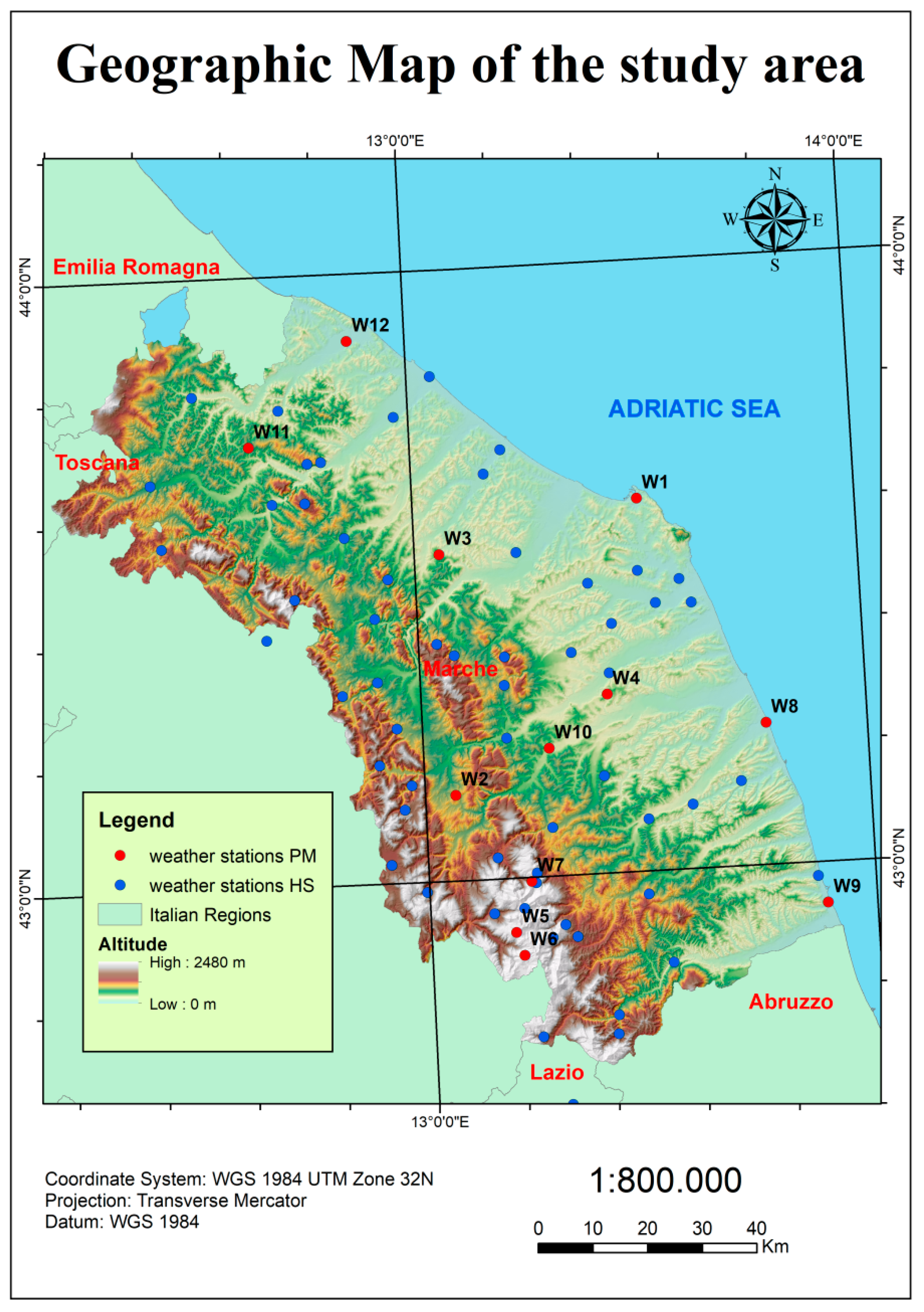
Furthermore, the homogeneity of the data was evaluated for all the variables investigated, since the sensors are very sensitive and a lack of calibration could produce relevant errors, solved by the homogeneity analysis. In some cases, it was also necessary to reconstruct the data.

2.1. Study Area

This study was carried out in the Adriatic side of Central Italy, specifically in the Marche region. This territory is not homogeneous, with a mountainous part (Appennine chain) to the west with peaks over 2000 m; moving eastwards, after a wide hilly belt, it comes to the Adriatic coast. This area is a transition point between the Mediterranean climate (Csa), typical of the southern part of Italy, and the humid subtropical (Cfa) or temperate oceanic climate (Cfb) or high-altitude climate (H) [36] one, widespread in most parts of the territory. The study area shows average temperatures of almost 14 °C, with a significant increase of 0.5 °C in the last 30 years on average, due to climate change. This has allowed the coastal areas and nearby territories of the region to reach, and in some cases exceed, 16 °C of average annual temperature [38]. In the same way, a certain historical trend towards a decrease in rainfall in the area has been highlighted, especially in the summer months; this change is determining an extension of the Mediterranean climate in the area [39]. In order to estimate the ET0 in the area, 12 weather stations with the necessary requirements for the calculation using the PM method and 58 for the calculation using the HS method after the calibration have been selected (Figure 1).

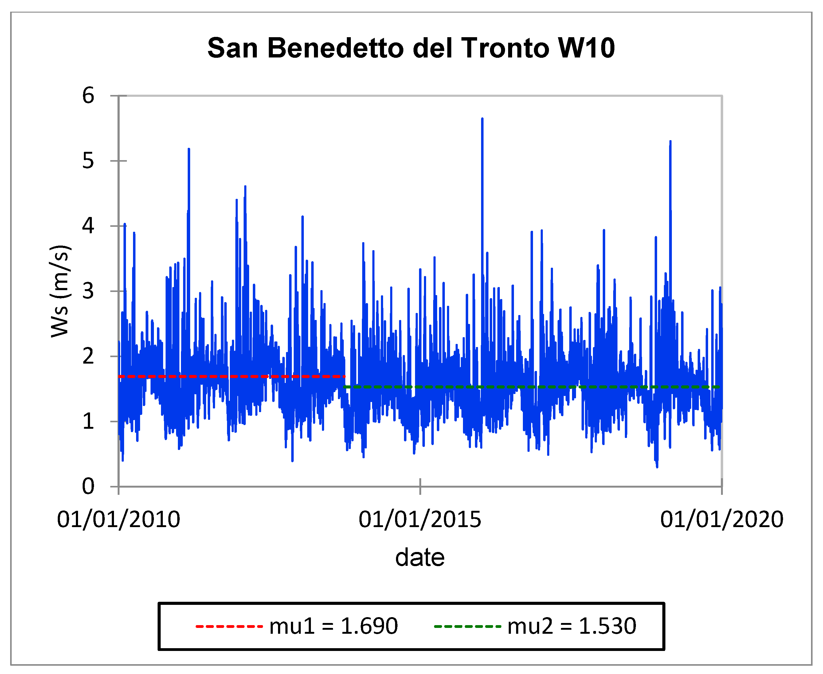
2.2. Quality Control, Homogenization and Reconstruction of Climate Data

The gross error checking test allowed us to remove all values outside the range of existence, including both values that are physically impossible and those that are impossible for the reference climate zone. The values identified at this stage are not flagged, but immediately removed. For the variables investigated the values chosen were the following:

• RH (Relative Humidity), from 1% to 100%;
• Ws (Wind speed), from 0.1 to 75 m/s [40];
• Rs (Global solar radiation), 0.03H0 < H < H0 [41,42];
• Tm (Mean temperature), from −40 to +50 [36,43].

The time consistency check analyzes the data of a historical time series, evaluating the maximum possible variability for a given parameter for continuous days or the minimum possible variability between continuous days (persistence) [44]. Thus, the time consistency check or temporal consistency check can be divided into two different controls:

• Persistence check;
• Maximum variability check.

All climate parameters were tested temporally in order to identify the persistence. A value that was repeated at least 3 times was considered a persistence [41].

After the persistence check, the maximum variability test was performed only for mean, maximum, and minimum temperatures. The reason is related to a poor relationship between contiguous days for humidity, solar radiation, and wind, which can have large variations that are difficult to identify as errors or correct values, as well as a spatial relationship that is not linear as in the case of temperature. The maximum variability test was performed on the basis of the relationship established by Zahumenský et al. [45] adapted for the daily period.

The spatial consistency check allowed possible malfunctions or systematic errors of the weather station under investigation (candidate) to be identified, according to some control weather stations located near the candidate one. In this case, linear regression was used as a method of evaluating spatial consistency, because of the speed of execution, as well as the precision of a method based on the mutual correlation of weather stations in respect to proximity relationships not always verified for variables such as relative humidity or wind [46]. For each candidate weather station, the five most correlated were chosen on the basis of the Pearson correlation coefficient. Subsequently, a linear regression was made taking into account the five weather stations acting as an independent variable, in order to reach the expected value for the dependent one. The predicted value of the dependent variable was compared with the real value by evaluating the residuals for each single daily value and evaluating it based on the arbitrarily chosen confidence interval with a level of significance of 99%. Only for solar radiation in addition to this method, due to some uncertainties in absolute measurements, was the spatial consistency evaluated by comparing the measured values with PVGIS (photovoltaic Geographic Information System)–SARAH (https://ec.europa.eu/jrc/en/PVGIS/downloads/SARAH (accessed on 12 February 2021)). The HELIOSAT-SARAH satellite is managed by the intergovernmental organization EUMETSAT and allows for the measurement of several parameters such as solar surface irradiance, surface direct irradiance (direct horizontal and direct normalized), sunshine duration, spectral information, and effective cloud albedo derived from satellite-observations of the visible channels of the MVIRI and the SEVIRI instruments, placed onboard the geostationary Meteosat satellites. Satellite data are available from 1983 to 2017 and monitor a range from ±65° north latitude to ±65° south latitude, with a resolution of 0.05° × 0.05°. In this study, data from 2010 to 2017 (last year of data availability) were compared and weather stations showing values exceeding 10% (significantly affecting the estimation of ET0) compared to SARAH model data were homogenized based on their historical ratios. A difference of more than 1 MJ/m² was considered too discordant and the values were modified by homogenizing them basing on their historical relationship with the SARAH data.

Annual calibrations of sensors should be usually performed, but sometimes this procedure is neglected and when the calibration is performed it may be necessary to homogenize most of the data collected. The homogeneity assessment was carried out not only for solar radiation, for which satellite data were used for homogenization, but also for the other variables which were homogenized by taking into account the ratios within the time series. The homogeneity analysis was performed with different tests: Pettitt, SNHT (Standard Normal Homogeneity Test), Buishand, and Von Neumann. At the end of the analysis, the Pettitt’s test was chosen because it is very versatile, accurate in identifying breakpoints, and because it does not require assumptions about data distribution as does a non-parametric test [47,48,49].

In order to solve any inhomogeneity, a reference time series was created to correct the candidate series based on their historical ratios. The reference series was calculated through a simple IDW (inverse distance weighted) interpolation [50].

Subsequently, the same ratio of the homogeneous period between the candidate time series and the reference one was applied to the inhomogeneous period of the candidate one, allowing the reconstruction. Concerning the “Ws” parameter, it required homogenization to ensure that all data were measured as required by the PM method at the height of 2 m above the ground level. In order to homogenize these data, the following formula was used [1,51]:

$$u_2=u_h\lfloor 4.87/\ln \left(67.8\mathrm{h}+5.42\right)\rfloor$$

(1)

• $u_2$ = wind speed 2 m above the ground m/s⁻¹;
• $u_h$ = measured wind speed h m above the ground m/s⁻¹;
• $h$ = height of the measurement above the ground.

All the parameters investigated highlighted some missing data, besides these “holes” increased after their validation. Therefore, it was necessary to reconstruct daily data using the same procedure adopted for the spatial consistency analysis, i.e., the multiple linear regression. This statistical technique has been used because in the case of parameters such as wind speed, solar radiation, and humidity the correlation is not strictly dependent on proximity. Therefore, through multiple linear regression, the reference weather stations most correlated with the candidate one were chosen for the reconstruction. As far as temperature was concerned, spatial relations were influenced due to the proximity with other weather stations and in relation to altitude, as observed in previous studies. These specific cases were satisfactorily reconstructed using the co-kriging method.

2.3. Methods for ET0 Calculation

There were some essential intermediate procedures and formulas required to solve the equation chosen to calculate ET0 based on the PM method [26,52,53,54,55,56,57,58,59]. Below is PM simplified (PM) equation presented in FAO-56 [1]:

$$E{T}_0=\frac{0.408\Delta \left(R_n-G\right)+\gamma \frac{C_n}{T+273}{u}_2\left(e_s-e_a\right)}{\Delta +\gamma \left(1+C_d{u}_2\right)}$$

(2)

• C_n = the numerator constant for the reference crop type and time step;
• C_d = the denominator constant for the reference crop type and time step;
• R_n = net radiation;
• u₂ = wind speed 2 m above the ground (m/s⁻¹);
• ∆ = slope of saturation vapor pressure curve at mean temperature (KPa °C⁻¹);
• γ = theoretical psychrometric constant;
• e_s = mean saturation vapour pressure at the air temperature T(KPa);
• e_a = actual vapour pressure derived from RH mean;
• G = soil heat flux (MJ m⁻² day⁻¹).

In addition, a standardized ET0 equation was performed [60] in order to obtain standardized values for low crops (0.12 m, such as grass in cold weather). Finally, standardized values were established for C_n and C_d:

$$E{T}_{0s}=\frac{0.408\Delta \left(R_n-G\right)+\gamma \frac{900}{T+273}{u}_2\left(e_s-e_a\right)}{\Delta +\gamma \left(1+0.34u_2\right)}$$

(3)

The original equation cPM was used in the case of mountain weather stations since remote sensing analyses showed an absence of vegetation for both Monte Bove (W5) and Monte Prata (W6); while in the case of Pintura di Bolognola (W8), the lack of vegetation was detected for the non-vegetable growing season. For this reason, the use of the standardized values for C_n and C_d, valid only for the presence of a 12 cm grass cover, would not have been correct. In order to also obtain a reliable ET0 calculation for mountain stations, the following equation was used [61,62,63,64,65]:

$$E{T}_0=\frac{\Delta \left(R_n-G\right)+\rho c_p\left(e_s-e_a\right)/r_a}{\Delta +\gamma \left(1+r_c/r_a\right)}$$

(4)

where:

$$\rho =\frac{1000\ast P}{T_{kv}\ast R}$$

(5)

• ρ = atmospheric density (Kg/m³);
• P = atmospheric pressure at elevation z (KPa);
• R = specific gas constant 287 (J Kg⁻¹ K⁻¹);
• T_kv = virtual temperature (K).

$$T_{kv}=T_k\left(1-0.378\frac{e_a}{P}\right)$$

(6)

• T_k = absolute temperature (K) 273 + Tmean (°C);
• P = atmospheric pressure at elevation z (KPa).

$$r_c=\frac{R_l}{0.5 LAI}$$

(7)

• R_l = average daily (24 h) stomata resistance of a single leaf (s m⁻¹);
• LAI = leaf area index.

$$LAI=24h_c$$

(8)

h_c = crop height (m) = 0.5–0.15.

$$r_a=\frac{ln\left(\frac{z_m-d}{z_{om}}\right)\ast ln\left(\frac{z_h-d}{z_{oh}}\right)}{k^2{U}_z}$$

(9)

• r_a = aerodynamic resistance (s m⁻¹);
• z_m = height measurement (m);
• z_h = height temperature and humidity measurements (m);
• k = Von Karman constant (0.41);
• U_z = wind speed measurements at height zm (m s⁻¹);
• d = zero plane displacement of wind profile (m).

$$d=\frac{2}{3}{h}_c$$

(10)

zom = roughness parameter for momentum (m).

$$z_{om}=0.123\ast h_c$$

(11)

zoh = roughness parameter for heat and water vapor (m).

$$z_{oh}=0.0123\ast h_c$$

(12)

Parallel to this calculation performed with the PM equation, the ET0 was also calculated through the HS equation, in order to calibrate the HS with the PM:

$$E{T}_0=0.0023\ast 0.408\ast R_a\ast \left(T_{mean daily}+17.8\right)\ast {\left(T_{Max daily}-T_{daily }\right)}^{0.5}$$

(13)

• 0.0023 = empirical Hargreaves coefficient (HC);
• 17.8 = empirical temperature Hargreaves constant (TH);
• 0.5 = empirical Hargreaves exponent.

2.4. Data Analysis and Interpolations

Initially, an analysis was performed on the data to assess the differences between the HS and PM methods. The 12 weather stations analyzed were compared by calculating the ET0 with both the HS and PM methods and evaluating the differences, in particular the difference in percentage over the decade 2010–2020. It was also calculated the annual confidence interval of each weather station, in order to assess the uncertainty in the inter-annual relationship between the two methods. Thus, for each year the differences in percentage were calculated and from these values a 95% confidence interval was obtained using the analysis of the standard deviation from the mean, in order to obtain an average difference value between the two methods, at least among the weather stations investigated. However, one of the most important steps of this study is that of the interpolation, which allows us to spatialize the data even where direct measurements are absent. Interpolation was performed to assess the distribution of both HC and ET0 after calibration; therefore, geostatistical methods were used to assess the error in estimating values. It follows that compared to deterministic methods there was a greater awareness and significant improvement in the efficiency of the model [66,67,68]. In this context, due to the excellent performance experienced over the years in many fields of application, the kriging method was chosen. All spatial interpolations were performed via GIS software, comparing iteratively three different methods for HC: ordinary kriging (OK), empirical Bayesian kriging (EBK), and ordinary cokriging (OCK) [69]. Instead, for the calculation of ET0 the methods were: simple kriging (SK), empirical Bayesian kriging (EBK), and simple cokriging (SCK). As the independent variable for SCK and OCK, altitude was chosen, while the simple method was preferred to ordinary when the number of samples was greater. The simple kriging is based on the assumption which considers the mean known over the whole area of study. It is also necessary to specify that the data were declustered by dividing the study area into square cells with a 17-km side. The results of the performance of the different predictive models were evaluated using cross-validation through some statistical indicators that allowed us to evaluate the correctness of the interpolation, with the procedure of leave-one-out: root mean square error (RMSE), mean standardized error (MSE), root mean square standardized error (RMSSE), and average standard error (ASE) [66]. In order to accurately assess the best performing methods, standardized indicators were taken into account: MSE represents the average of standardized errors and should be close to 0, in addition to RMSSE, which indicates how far the expected values deviate from the real value, the value 1 representing the perfect match between predicted and measured. The value with the lowest residual was considered the most reliable for interpolation purposes.

3. Results

3.1. Quality Control

Quality control prior to ET0 analysis allowed the removal of numerous incorrect data for each individual variable. In this case, a table with all the parameters investigated and all the weather station considered was reported (

Table 2. Summary of percentages of data deleted after quality checks (G. = gross error checking; T. = temporal consistency; S. = spatial consistency) and percentages of reconstructed data (R. = reconstructed data).

Check		Weather Stations
C. Par.	%	W1	W2	W3	W4	W5	W6	W7	W8	W9	W10	W11	W12
TMax	G.	0.0	0.0	0.0	0.0	0.0	0.0	0.0	0.0	0.0	0.0	0.0	0.0
TMax	T.	0.1	0.0	0.1	0.1	0.0	0.2	0.1	0.1	0.0	0.0	0.0	0.0
TMax	S.	0.5	1.9	0.6	0.4	1.8	0.4	0.6	1.0	0.5	0.8	1.1	1.1
TMax	R.	7.0	5.7	3.4	3.2	10.9	9.8	10.0	9.8	9.3	3.7	9.9	9.9
Tmean	G.	0.0	0.0	0.1	0.0	0.0	0.0	0.0	0.0	0.0	0.0	0.0	0.0
Tmean	T.	0.0	0.0	0.0	0.0	0.0	0.1	0.0	0.0	0.0	0.0	0.0	0.0
Tmean	S.	1.8	1.8	1.1	0.4	1.8	0.6	0.4	1.0	1.0	0.8	0.4	1.0
Tmean	R.	7.0	5.7	3.4	3.2	10.9	9.8	10.8	9.8	9.3	3.7	3.3	9.9
Tmin	G.	0.0	0.0	0.0	0.0	0.0	0.0	0.0	0.0	0.0	0.0	0.0	0.0
Tmin	T.	0.2	0.1	0.0	0.1	0.0	0.2	0.1	0.0	0.0	0.0	0.2	0.0
Tmin	S.	0.5	1.9	0.6	0.4	1.8	0.4	0.6	1.0	0.5	0.8	0.4	1.1
Tmin	R.	7.0	5.7	3.4	3.2	10.9	9.8	10.0	9.8	9.3	3.7	3.3	9.9
RH	G.	0.0	0.0	0.0	0.0	0.0	0.0	0.0	0.0	0.0	0.1	0.0	0.0
RH	T.	0.0	0.2	0.0	0.0	1.1	0.4	0.8	1.4	0.0	0.0	0.0	0.0
RH	S.	0.8	0.7	0.4	0.7	1.1	3.4	1.4	1.1	0.5	2.0	0.8	1.2
RH	R.	1.3	1.6	1.5	2.0	5.7	6.2	7.3	5.2	5.2	3.1	1.3	3.2
Rs	G.	1.5	0.6	0.9	1.7	9.6	0.1	0.5	1.7	0.2	0.1	0.2	1.1
Rs	T.	0.0	0.0	0.0	0.0	0.0	0.0	0.0	0.0	0.0	0.0	0.0	0.0
Rs	S.	1.1	1.6	1.3	1.8	2.5	1.2	1.9	7.4	1.8	1.2	1.0	1.4
Rs	R.	3.7	3.5	3.4	15.2	15.1	3.7	2.8	12.8	7.7	2.5	1.9	5.2
Ws	G.	0.4	0.2	0.0	4.2	3.4	2.9	2.2	0.1	0.0	2.9	0.2	0.0
Ws	T.	0.0	0.0	0.0	0.0	0.0	0.0	0.0	0.0	0.0	0.0	0.0	0.0
Ws	S.	0.9	0.7	0.7	1.1	2.0	1.9	1.4	0.5	0.7	1.4	0.9	0.5
Ws	R.	1.9	2.1	1.8	4.1	8.8	9.2	7.2	3.5	5.7	5.9	1.5	3.3

).

In the case of wind speed, a measurement discrepancy was detected in only one weather station, because the sensor was located 10 m above the ground surface, while the PM’s formula required a 2-m height. Thus, the W4 has been adjusted following the Equation (4) [50]. In addition, despite the quality controls, in some cases very important systematic errors were detected in the time series (Rs, Ws). This fact led to some important changes in the data in order to obtain a more reliable value of ET0. In particular, a great underestimation was found for the parameter Ws and for the weather station W10, which was then solved by collecting data from a nearby weather station not included in the analysis. A lack of homogeneity in the values for W10, perhaps due to a small displacement of the sensor, was homogenized with a reference weather station created through an IDW among the neighboring ones (Figure 2).

Finally, other systematic errors were detected for some weather stations with regard to solar radiation, after the comparison with the climate data records of SARAH satellite (

Table 3. Differences in the annual average from 2010 to 2017 of the solar radiation values measured by pyranometers (Rs-measured W. Station) and those measured by the satellite HELIOTSAT-SARAH (Rs-measured SARAH).

Daily Average	Weather Stations
MJ/m2	W1	W2	W3	W4	W5	W6	W7	W8	W9	W10	W11	W12
Rsmeasured SARAH	14.8	14.1	14.3	14.6	12.4	13.2	12.6	15.0	15.2	15.4	14.2	14.6
Rsmeasured W. Station	14.5	14.1	14.1	14.1	15.2	15.8	14.7	15.3	15.3	14.1	15.1	12.9

).

Overestimations of solar radiation were detected for all the mountain weather stations (W5, W6, W7) and for the ones at San Benedetto (W10) and Villa Fastiggi (W12). The present study focused heavily on the reliability of climate data through a long and detailed validation procedure, which led to the elimination of about 1% of Tmax, Tmin, Tmean, and RH data, 3.5% for Rs, and 2.4% for Ws. In addition, some data that had some very relevant holes in the historical time series were reconstructed, in particular about 7% of the data for Tmax, Tmin, Tmean, and Rs, 3.6% for RH, and 4.6% for Ws.

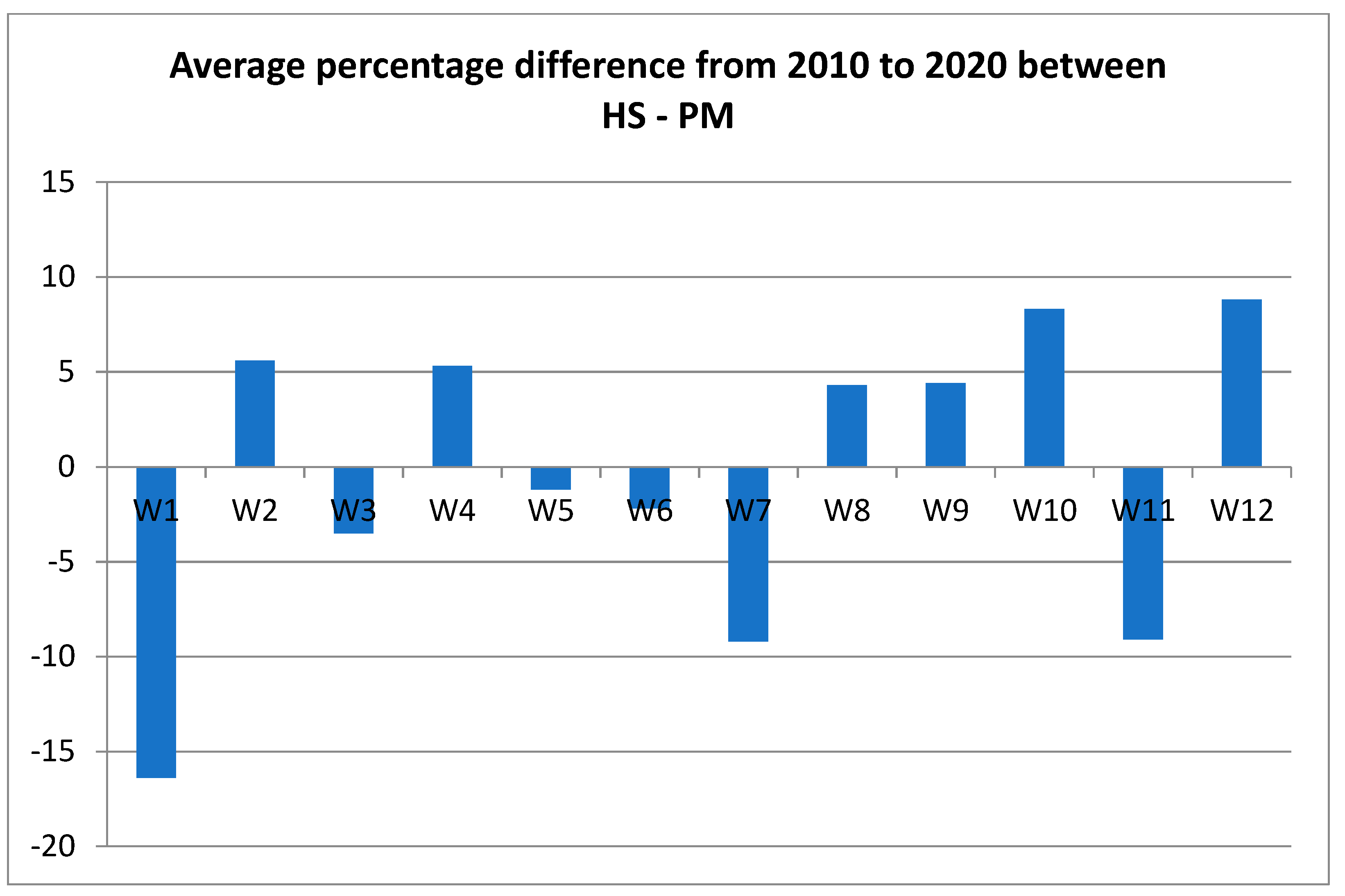
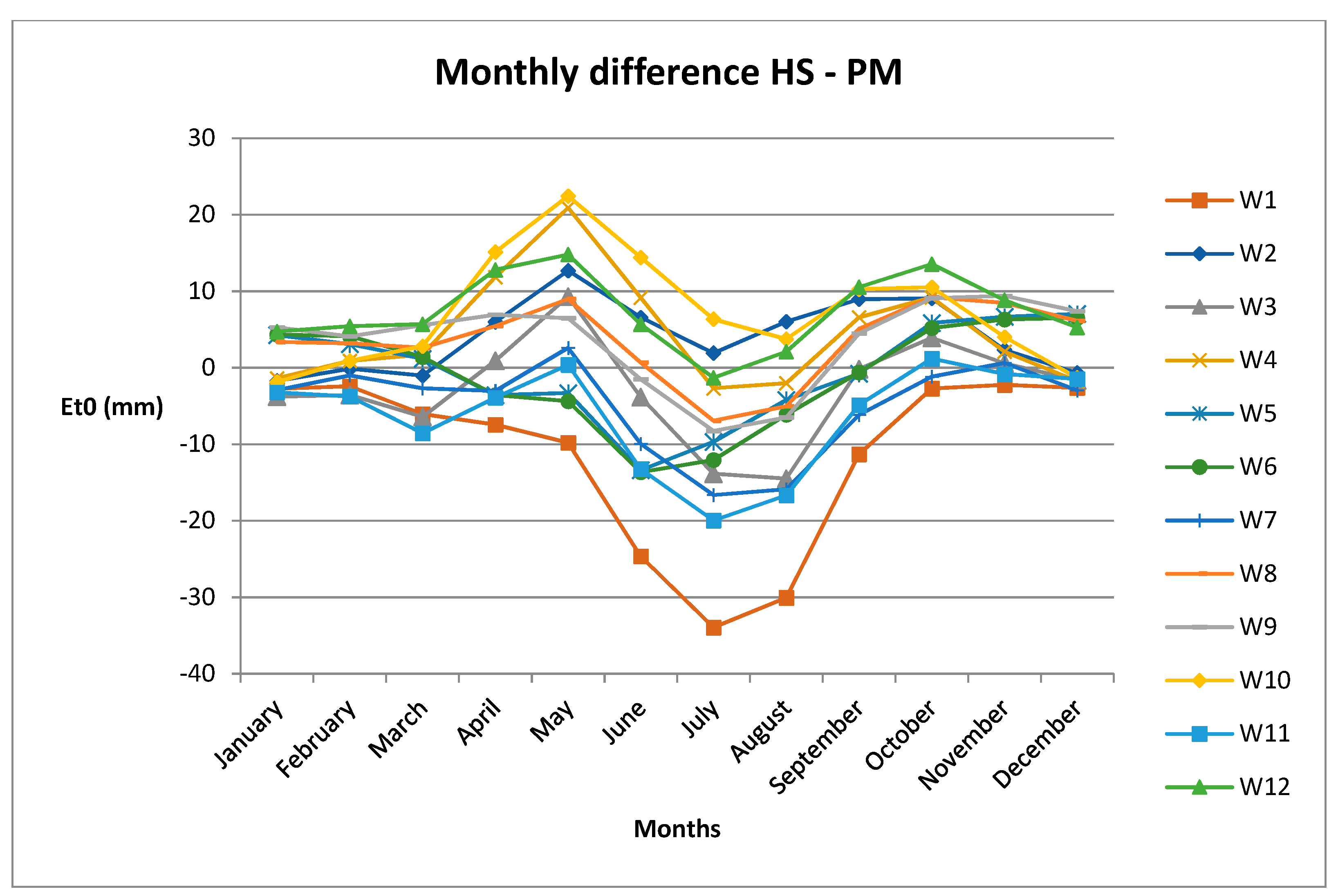
3.2. Comparison between Penmann Monteith’s and Hargreaves ET0 Calculation Methods

The daily ET0 was calculated for both PM and HS methods in order to evaluate the differences and subsequently correct the coefficient of the method that required fewer parameters (HS). First, annual and monthly averages in the range 2010–2020 for each weather station were calculated for both methods (

Table 4. Average annual and monthly ET0 over the period 2010–2020 calculated using the Penman–Monteith (PM) and the Hargreaves (HS) method; W5, W6, and W7 are calculated with the complete Penman–Monteith (cPM).

ET0	P.	W1	W2	W3	W4	W5	W6	W7	W8	W9	W10	W11	W12
PM	Jan	23.9	21.4	24.8	25.5	8.5	8.9	18.8	20.8	20.2	25.1	21.8	18.5
PM	Feb	31.0	26.8	32.0	32.5	13.4	13.6	21.7	28.9	29.4	31.2	28.4	26.8
PM	Mar	60.0	53.4	62.6	62.6	29.4	30.5	39.9	57.4	55.8	60.6	57.4	58.2
PM	Apr	84.5	75.2	84.5	84.0	50.0	53.5	59.9	81.1	79.2	81.1	79.8	81.4
PM	May	113.4	95.6	107.3	106.9	68.4	72.1	73.9	107.6	108.3	105.9	102.7	110.8
PM	Jun	149.3	131.2	150.2	147.5	96.8	99.5	107.9	140.9	140.7	148.1	142.3	149.0
PM	Jul	166.1	149.7	172.6	171.6	106.2	110.3	126.2	159.5	158.9	173.5	159.7	164.1
PM	Aug	145.9	130.7	153.9	155.2	92.0	95.2	113.5	140.9	141.1	153.9	139.3	141.2
PM	Sep	90.2	75.8	88.1	91.7	53.9	55.2	66.4	86.6	87.0	88.7	81.1	83.0
PM	Oct	50.5	41.5	46.9	48.8	27.5	28.7	39.0	46.3	47.1	47.1	43.0	42.8
PM	Nov	29.4	24.1	26.5	29.0	11.0	12.0	20.3	23.5	23.8	26.5	24.3	21.9
PM	Dec	22.5	20.3	22.1	25.7	6.3	6.8	18.7	17.6	17.6	24.1	19.5	16.9
PM	Ann	967	846	971	981	563	586	706	911	909	966	899	915
ET0	P.	W1	W2	W3	W4	W5	W6	W7	W8	W9	W10	W11	W12
HS	Jan	21.1	19.6	21.0	24.1	12.8	13.2	15.9	24.1	25.4	23.3	18.6	23.2
HS	Feb	28.6	26.7	28.4	33.4	16.5	17.7	20.7	32.1	33.5	32.0	24.6	32.2
HS	Mar	54.0	52.3	56.1	64.3	30.5	31.9	37.2	60.0	61.4	63.4	48.8	63.9
HS	Apr	77.0	81.1	85.4	95.8	46.4	50.0	56.8	86.6	86.2	96.2	75.9	94.1
HS	May	103.6	108.3	116.6	127.8	65.1	67.7	76.5	116.6	114.7	128.4	103.0	125.6
HS	Jun	124.6	137.8	146.3	156.7	83.4	85.8	97.9	141.6	139.2	162.5	129.0	154.7
HS	Jul	132.2	151.6	158.7	168.9	96.6	98.3	109.5	152.6	150.6	179.8	139.8	162.8
HS	Aug	115.8	136.7	139.4	153.2	87.7	89.0	97.6	135.8	134.6	157.6	122.6	143.2
HS	Sep	78.9	84.8	87.9	98.3	53.1	54.6	60.2	91.7	91.4	98.9	76.2	93.5
HS	Oct	47.8	50.6	50.8	58.0	33.4	33.9	37.8	55.5	56.2	57.7	44.2	56.3
HS	Nov	27.1	26.4	27.0	31.0	17.6	18.3	20.9	32.0	33.1	30.5	23.4	30.7
HS	Dec	19.9	19.6	20.5	23.9	13.3	13.3	15.8	23.7	24.9	22.7	18.1	22.2
HS	Ann	830	895	938	1035	556	574	647	952	951	1053	824	1003

).

This first analysis (Table 4) showed that the ET0 calculated with HS was very similar to the values obtained with the cPM equation at mountain weather stations, with values that only differed by a few mm annually. Other weather stations, on the other hand, were subject to fluctuations that could be significant and not very well correlated with the morphology of the area (Figure 3;

Table 5. Average percentage difference from 2010 to 2020 between the two methods of calculation (HS-PM) of ET0 for each weather station (dif. 2010–2020); 95% confidence interval between years for each weather station (95% conf. int.).

W. Station	W1	W2	W3	W4	W5	W6	W7	W8	W9	W10	W11	W12
dif. 2010–2020	−16.4	5.6	−3.5	5.3	−1.2	−2.2	−9.2	4.3	4.4	8.3	−9.1	8.8
95% conf. int.	±5.0	±3.0	±4.7	±4.5	±2.9	±1.8	±2.4	±2.4	±2.6	±3.7	±3.1	±2.3

). In addition, the Pearson correlation coefficient between the annual values obtained with the HS and PM methods was calculated to be 0.92. Although it showed good agreement, there was the possibility of observing appreciable differences.

The monthly difference between the two methods was also assessed. The graph in Figure 3 shows how the different weather stations followed a common pattern, indicating the monthly correlation, but also a systematic error between the methods. There was evidence of underestimation of evapotranspiration by the HS method in the summer months (June, July, August) and overestimation in spring (April, May) and autumn (October, November).

In this context, in order to minimize the differences between the PM and the HS methods, the coefficient HC was iteratively modified reaching the minimum RMSE value comparing the PM with the HS modified (

Table 6. Empirical coefficient of Hargreaves HC for each interval (Jan, Feb, Mar, etc.) multiplied by 10-3, adapted to the investigated weather stations (W1, W2, …) in order to minimize the difference between the HS ET0 equation and that of PM.

W.S.	W1	W2	W3	W4	W5	W6	W7	W8	W9	W10	W11	W12
Jan HC	2.6	2.5	2.7	2.4	1.6	1.6	2.7	2.0	1.8	2.5	2.7	1.8
Feb HC	2.5	2.3	2.6	2.2	1.9	1.8	2.4	2.1	2.0	2.2	2.7	1.9
Mar HC	2.6	2.3	2.6	2.2	2.2	2.2	2.5	2.2	2.1	2.2	2.7	2.1
Apr HC	2.5	2.1	2.3	2.0	2.5	2.5	2.4	2.2	2.1	1.9	2.4	2.0
May HC	2.5	2.0	2.1	1.9	2.4	2.4	2.2	2.1	2.2	1.9	2.3	2.0
Jun HC	2.8	2.2	2.4	2.2	2.7	2.7	2.5	2.3	2.3	2.1	2.5	2.2
Jul HC	2.9	2.3	2.5	2.3	2.5	2.6	2.6	2.4	2.4	2.2	2.6	2.3
Aug HC	2.9	2.2	2.5	2.3	2.4	2.5	2.7	2.4	2.4	2.2	2.6	2.3
Sep HC	2.6	2.1	2.3	2.1	2.3	2.3	2.5	2.2	2.2	2.1	2.5	2.0
Oct HC	2.5	1.9	2.2	2.0	2.0	2.0	2.3	2.0	2.0	1.9	2.3	1.8
Nov HC	2.5	2.2	2.4	2.2	1.6	1.6	2.2	1.7	1.7	2.1	2.5	1.7
Dec HC	2.7	2.3	2.4	2.4	1.3	1.3	2.6	1.8	1.7	2.4	2.5	1.8
Ann HC	2.7	2.1	2.4	2.2	2.3	2.3	2.5	2.2	2.2	2.1	2.5	2.1

).

This procedure was preparatory to obtain a map of the distribution of the HC in the study area, in order to use all weather stations with the detection of Tmax, Tmean, and Tmin, for ET0 calculation.

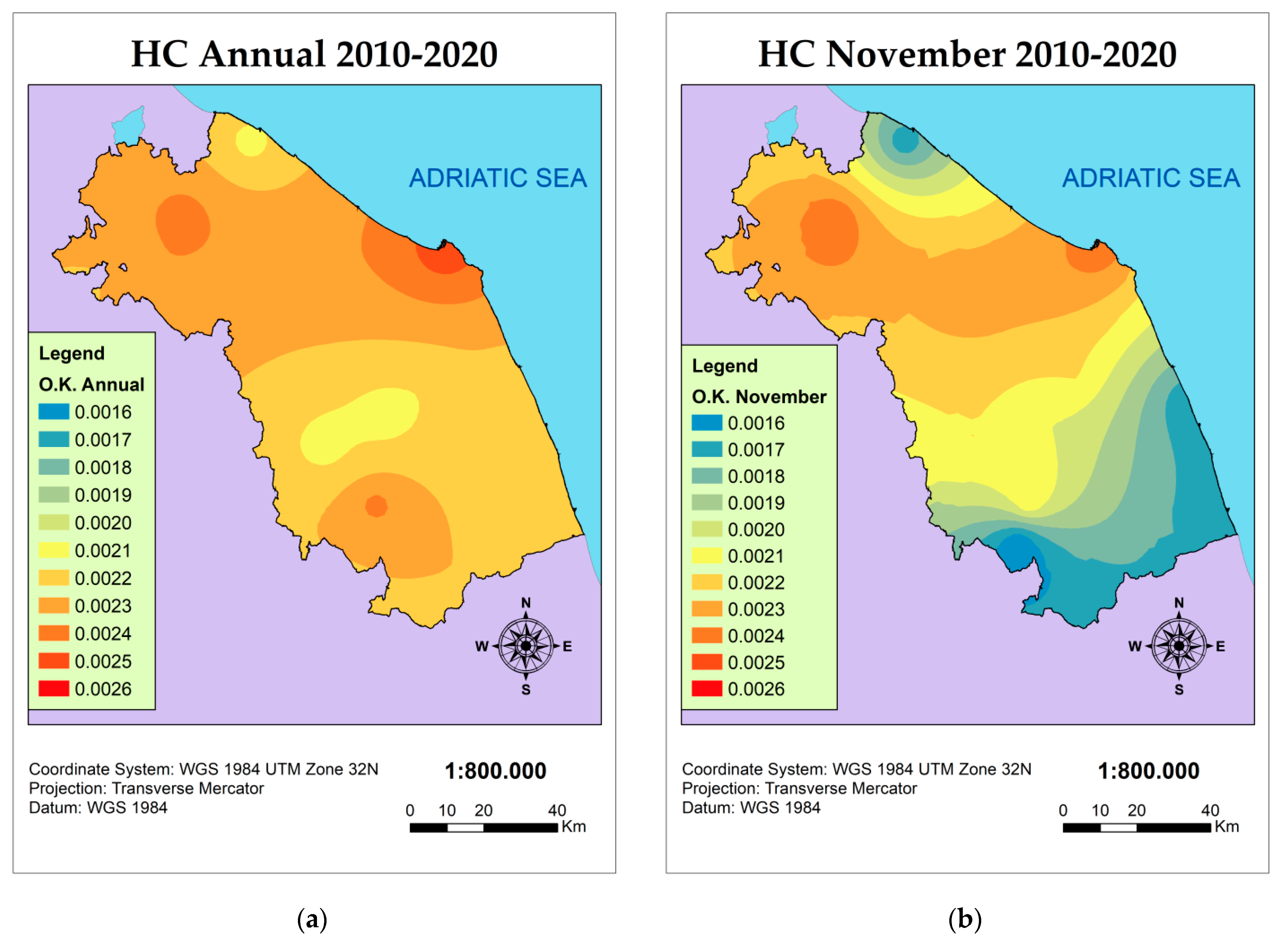
3.3. Interpolation of the Hargreaves Coefficient HC

The interpolation to obtain the HC was assessed for each month and annually with the three methods: OK, EBK, and OCK. The independent variable for OCK was altitude which showed the best correlation performance between other geographical variables investigated (latitude, exposure, slope, distance from the watershed line, etc.).

The table (

Table 7. Empirical coefficient of Hargreaves HC for each interval (Jan, Feb, Mar, etc.) multiplied by 10⁻³, adapted to the investigated weather stations (W1, W2, …) in order to minimize the difference between the HS ET0 equation and that of PM. The best interpolation for each time interval is highlighted in red.

	RMSE	MSE	RMSSE	ASE		RMSE	MSE	RMSSE	ASE
OK Jan	0.00042	−0.02058	0.99948	0.00048	OK Feb	0.00029	−0.01014	1.00919	0.00027
OCK Jan	0.00042	0.05025	0.97203	0.00045	OCK Feb	0.00030	0.01955	1.04040	0.00028
EBK Jan	0.00043	0.01265	0.91740	0.00047	EBK Feb	0.00031	0.00523	0.94670	0.00031
OK Mar	0.00022	−0.01469	0.99964	0.00021	OK Apr	0.00023	−0.00270	1.01601	0.00022
OCK Mar	0.00024	0.01448	1.18229	0.00019	OCK Apr	0.00019	0.00270	0.87131	0.00019
EBK Mar	0.00023	0.02283	0.99274	0.00022	EBK Apr	0.00022	−0.00105	0.93277	0.00021
OK May	0.00018	−0.03791	0.99523	0.00016	OK Jun	0.00023	−0.00484	1.00051	0.00023
OCK May	0.00018	−0.00693	0.90759	0.00018	OCK Jun	0.00019	0.02802	0.82823	0.00020
EBK May	0.00021	−0.01225	0.95158	0.00019	EBK Jun	0.00023	0.00661	0.91972	0.00021
OK Jul	0.00020	−0.01011	1.00730	0.00019	OK Aug	0.00022	−0.02360	0.99735	0.00022
OCK Jul	0.00020	−0.04213	1.15612	0.00017	OCK Aug	0.00022	−0.04539	0.97564	0.00023
EBK Jul	0.00021	0.02720	1.01468	0.00020	EBK Aug	0.00022	0.02864	1.01629	0.00022
OK Sep	0.00021	0.00201	1.06929	0.00019	OK Oct	0.00025	−0.03778	1.00047	0.00024
OCK Sep	0.00021	−0.00863	1.06453	0.00019	OCK Oct	0.00023	0.00923	1.10969	0.00020
EBK Sep	0.00021	0.06140	1.02250	0.00020	EBK Oct	0.00023	0.06093	0.99900	0.00022
OK Nov	0.00034	−0.00022	0.98974	0.00033	OK Dec	0.00041	−0.00885	0.99847	0.00046
OCK Nov	0.00033	0.03827	0.96585	0.00033	OCK Dec	0.00045	0.05236	0.91954	0.00051
EBK Nov	0.00035	−0.01738	0.97694	0.00034	EBK Dec	0.00047	0.01078	0.91282	0.00052
OK Year	0.00021	0.00349	1.07832	0.00019
OCK Year	0.00022	0.00506	1.10586	0.00019
EBK Year	0.00021	−0.03607	1.11018	0.00021

) shows that OK was the best way to interpolate the HC coefficient values on a monthly and annual scale. The success of the OK highlighted the failure, due to the lack of correlation with the independent variable, of the OCK that is usually (in the presence of correlation with the dependent variable) very accurate. These interpolations were functional for knowing the HC for each month and annually (Figure 4) for each point in the surface of the study area.

As a result, the 58 additional weather stations chosen to calculate the ET0 with the HS method were assumed in the HS equation the value HC generated by the interpolation. This consequently resulted in a calibration of the HS method with the PM method for all weather stations and the cPM method in the case of mountain weather stations.

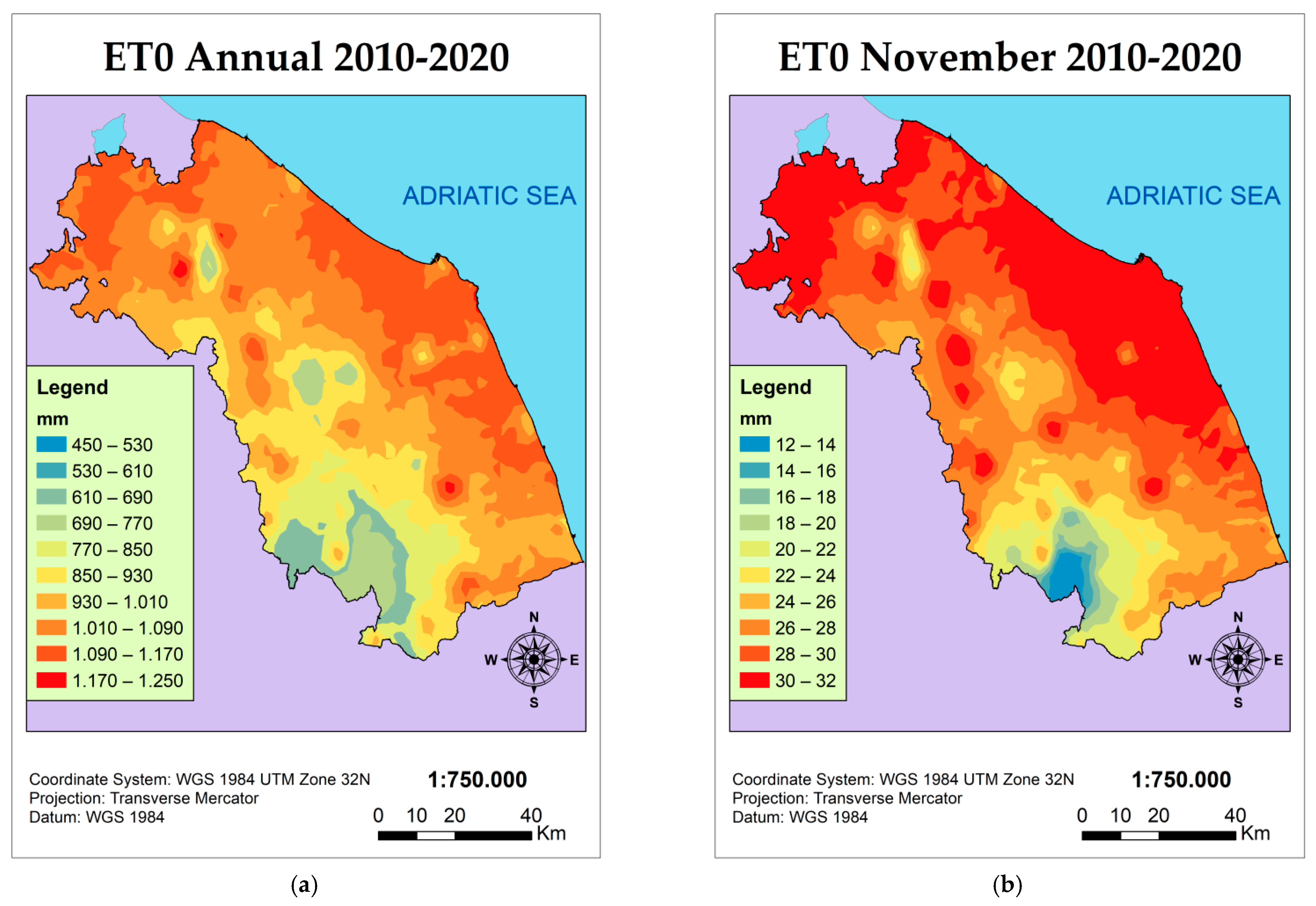
3.4. Calculation of ET0

The adjustment of the HC allowed the definition of ET0 in the study area with many more measurement points, allowing a more accurate calculation. As in the case of HC interpolation, the best interpolation method for ET0 was iteratively evaluated.

Table 8. Cross validation results for each time interval and for each geostatistical method used; the best method for each interval is highlighted in red.

	RMSE	MSE	RMSSE	ASE		RMSE	MSE	RMSSE	ASE
SK Jan	3.61	−0.03116	0.689	5.57	SK Feb	4.54	−0.03681	0.902	5.30
SCK Jan	3.91	−0.00706	1.008	3.88	SCK Feb	4.79	−0.00116	0.993	4.82
EBK Jan	3.82	−0.01709	0.992	3.89	EBK Feb	4.75	−0.03228	0.987	4.86
SK Mar	8.49	−0.02914	0.839	10.63	SK Apr	11.35	−0.02982	0.854	13.83
SCK Mar	9.06	−0.00116	0.999	9.07	SCK Apr	11.85	−0.00483	0.985	12.02
EBK Mar	8.94	−0.03335	0.980	9.24	EBK Apr	11.80	−0.03532	0.978	12.20
SK May	14.62	−0.0.1844	0.837	17.74	SK Jun	19.79	−0.03059	0.866	23.58
SCK May	15.17	−0.01990	0.992	15.27	SCK Jun	20.69	−0.00257	0.99494	20.77
EBK May	14.96	−0.04320	0.984	15.35	EBK Jun	20.47	−0.03529	0.97856	21.11
SK Jul	22.11	−0.03417	0.849	27.02	SK Aug	19.65	−0.03368	0.871	24.15
SCK Jul	23.40	−0.00517	0.994	23.51	SCK Aug	20.49	−0.00556	0.991	20.67
EBK Jul	22.98	−0.03168	0.990	23.44	EBK Aug	20.15	−0.03273	0.986	20.65
SK Sep	11.64	−0.03121	0.862	14.46	SK Oct	6.98	−0.06199	0.929	7.73
SCK Sep	11.69	−0.04715	1.003	11.70	SCK Oct	6.87	−0.03277	1.000	6.83
EBK Sep	11.99	−0.03929	0.992	12.22	EBK Oct	7.12	−0.04362	0.987	7.28
SK Nov	3.95	−0.04198	0.912	4.87	SK Dec	3.32	−0.05343	0.884	4.05
SCK Nov	3.93	−0.00271	0.998	4.02	SCK Dec	3.20	−0.03497	0.998	3.23
EBK Nov	4.11	−0.03503	0.987	4.23	EBK Dec	3.33	−0.01604	0.984	3.43
SK Year	127.47	−0.03266	0.858	155.53
SCK Year	130.30	−0.04667	1.000	130.00
EBK Year	132.41	−0.03607	0.984	136.02

shows the results of the 3 methods analyzed SK, SCK, EBK.

Table 8 shows that the most accurate method was SCK, the result of a good correlation between ET0 and altitude. The EBK method also performed very well, and was easy to use due to the iterativity of the method, which was delegated to the software. This interpolation led to the production of 12 monthly maps and one annual one originating from the average of ET0 from 2010 to 2020. Two of the most significant maps are reported in Figure 5.

By observing the figures, it is possible to observe the great heterogeneity of the study area (Figure 6), where the ET0 range went from 450 mm to up to 1250 mm per year. The lowest values were reached in the south-western mountain area, while the highest were widely obtained in the north and in the coastal sector to the east.

4. Discussion

Data quality control is a very important part of a climate analysis and is the strength of this research, as it is the basis for all other approximations in the equations. The correctness of the climate data determines, as demonstrated by other studies [70,71], the accuracy of the ET0 estimation using the PM and cPM method, which otherwise cannot be considered reliable. The temperatures, also due to more effective preliminary validations, allowed us to have less erroneous data; in any case the same quality control procedure was performed for all other weather stations [37] involved in the calculation of ET0 with HS. The HS method, in a temperate climate on the border of the Mediterranean climate, at average latitudes, showed surprising results compared with previous studies [72,73]. In particular, only one weather station averaged over 10 years showed percentage differences between HS and PM greater than 10% (but less than 20%). This result highlighted substantial differences both with similar research carried out in other environments [72] and with research carried out in climatically related territories [73]. No systematic over- or underestimations of HS compared to PM were found in this research in contrast to what is often observed in the literature [74,75]. Besides, very interesting particularities were observed in the case of weather stations above 1200 m a.s.l., where HS was shown to be more accurate than the PM method and in great agreement with the cPM method. The cPM allowed for the accurate evaluation of mountain weather stations, where the vegetation was almost absent and consequently determined lower values of ET0. In this context, the value of HC was found to be variable from zone to zone, but certainly correlated with the various weather stations that have shown some agreement when close, with similar environmental and climate parameters. Furthermore, it was significant to note that the annual estimates of the two methods (cPM and HS without calibration) were very close in the case of the weather stations with the highest altitude, above 1800 m (−1.2- and −2.2-point percentage of difference). This observation clearly disagrees with much of the literature, which reports a significant weakness in the case of mountain weather stations [35,76]. The concordance between the two methods in this territory leads to evaluate the reasons that could be dictated by the climatic-environmental peculiarities that characterize it. The study area is in a transitional zone between temperate and Mediterranean climate. Furthermore, there is also a very unusual conformation of the territory, characterized by great environmental and altitudinal variations even at short distances with a moderate mitigating influence of the Adriatic Sea, due to its small size. In order to obtain a perfect calibration of the HS method from the PM, the HC was modified on a monthly and annual basis. From an annual point of view, it was possible to observe a non-substantial calibration, with maximum values of variation with respect to the standard coefficient [77] equal to ±0.0004. Some studies agree with this evidence [72], while others disagree and need greater calibrations [11]. The HC was interpolated over the entire study area, with GIS software, so that the added weather stations could enjoy the coefficients established in the calibration. HC interpolation compared various kriging methods (Table 7), which very often turned out to be among the best statistical methods of interpolation [78], allowed a good spatialization as it was possible to analyze from the cross validation (Table 7). The HC coefficient interpolated with OK was then attributed both on a monthly and annual scale to each weather station, making the calculation of ET0 with HS more accurate and more similar to PM and cPM results. Finally, the variable ET0 was spatialized through a SCK with altitude as independent variable, which proved to be the most accurate geostatistical method among those investigated (Table 8). The good relationship between ET0 and altitude has already been verified in the past, even in territories very different from the study area [79]. Some limitations of this research must be taken into account when critically analyzing the results. The first limit, unsurpassable at the moment, was the presence of only 12 weather stations for the analysis of the entire study area, using the PM and cPM method. Despite the appropriate data declusterization being performed, there were some under-sampled areas that may have shown slightly different results, both as HC and consequently as ET0. Furthermore, it would be appropriate to compare the results obtained by theoretical calculations, with experimental measurements by lysimeters, especially in mountain weather stations, where the ET0 was calculated using the cPM method instead of the simplified one. It follows that the limitations of this study were mainly technical.

5. Conclusions

Potential evapotranspiration is fundamental for accurately assessing water supply and crop needs and, mostly, for estimating the water budget of a given area. Very often different methods are observed to give different results even of hundreds of mm of ET0 for the same location. The resolution of the uncertainty in the estimation of ET0 by calculating the HC over the whole study area allows results to be obtained that are much more similar to the more refined PM and cPM method. Furthermore, a certain reliability of the HS method was observed, probably due to careful quality control operations on the original data. Of great interest was the excellent correlation detected between the uncalibrated HS method and the cPM in the case of mountain weather stations. Finally, a good correlation was observed regarding the ET0 parameter with the change in altitude, which led to better interpolation and could also be exploited in other areas in the future to improve the analysis. This research is intended to be the starting point for further analysis, which can use the correct ET0 calculation, even with low parameters, for various purposes. The calculation of potential evapotranspiration is indispensable for water resource management, giving a priority to any interventions and for agricultural planning of the territory, and obtaining a reliable value of the water needs of crops, which can discriminate the cultivation choices.

References

1. Allen, R.G.; Pereira, L.S.; Raes, D.; Smith, M. Crop. Evapotranspiration: FAO Irrigation and Drainage Paper 56; FAO: Rome, Italy, 1998; p. 20. [Google Scholar]
2. López-Urrea, R.; Montoro, A.; Mañas, F.; López-Fuster, P.; Fereres, E. Evapotranspiration and crop coefficients from lysimeter measurements of mature ‘Tempranillo’ wine grapes. Agric. Water Manag. 2021, 112, 13–20. [Google Scholar] [CrossRef]
3. Gentilucci, M.; Barbieri, M.; Burt, P. Climate and Territorial Suitability for the Vineyards Developed Using GIS Techniques. In Exploring the Nexus of Geoecology, Geography, Geoarcheology and Geotourism: Advances and Applications for Sustainable Development in Environmental Sciences and Agroforestry Research; Springer: Cham, Switzerland, 2019; pp. 11–13. [Google Scholar]
4. Moller, M.; Alchanatis, V.; Cohen, Y.; Meron, M.; Tsipris, J.; Naor, A.; Ostrovsky, V.; Sprintsin, M.; Cohen, S. Use of thermal and visible imagery for estimating crop water status of irrigated grapevine. J. Exp. Bot. 2007, 58, 827–838. [Google Scholar] [CrossRef] [Green Version]
5. Saadi, S.; Todorovic, M.; Tanasijevic, L.; Pereira, L.S.; Pizzigalli, C.; Lionello, P. Climate change and Mediterranean agriculture: Impacts on winter wheat and tomato crop evapotranspiration, irrigation requirements and yield. Agric. Water Manag. 2015, 147, 103–135. [Google Scholar] [CrossRef]
6. Kashyap, P.S.; Panda, R.K. Evaluation of evapotranspiration estimation methods and development of crop-coefficients for potato crop in a sub-humid region. Agric. Water Manag. 2001, 50, 9–25. [Google Scholar] [CrossRef]
7. Garcia, M.; Raes, D.; Jacobsen, S.E. Evapotranspiration analysis and irrigation requirements of quinoa (Chenopodium quinoa) in the Bolivian highlands. Agric. Water Manag. 2003, 60, 119–134. [Google Scholar] [CrossRef]
8. Tanasijevic, L.; Todorovic, M.; Pereira, L.S.; Pizzigalli, C.; Lionello, P. Impacts of climate change on olive crop evapotranspiration and irrigation requirements in the Mediterranean region. Agric. Water Manag. 2014, 144, 54–68. [Google Scholar] [CrossRef]
9. Jovanovic, N.; Israel, S. Critical Review of Methods for the Estimation of Actual Evapotranspiration in Hydrological Models. In Evapotranspiration-Remote Sensing and Modeling; IntechOpen Limited: London, UK, 2012. [Google Scholar]
10. Zhao, L.; Xia, J.; Xu, C.Y.; Wang, Z.; Sobkowiak, L.; Long, C. Evapotranspiration estimation methods in hydrological models. J. Geogr. Sci. 2013, 23, 359–369. [Google Scholar] [CrossRef]
11. Ravazzani, G.; Corbari, C.; Morella, S.; Gianoli, P.; Mancini, M. Modified Hargreaves-Samani equation for the assessment of reference evapotranspiration in Alpine river basins. J. Irrig. Drain. Eng. 2012, 138, 592–599. [Google Scholar] [CrossRef]
12. Thompson, J.R.; Green, A.J.; Kingston, D.G. Potential evapotranspiration-related uncertainty in climate change impacts on river flow: An assessment for the Mekong River basin. J. Hydrol. 2014, 510, 259–279. [Google Scholar] [CrossRef] [Green Version]
13. Duran-Encalada, J.A.; Paucar-Caceres, A.; Bandala, E.R.; Wright, G.H. The impact of global climate change on water quantity and quality: A system dynamics approach to the US–Mexican transborder region. Eur. J. Oper. Res. 2017, 256, 567–581. [Google Scholar] [CrossRef] [Green Version]
14. De Beurs, K.M.; Henebry, G.M.; Owsley, B.C.; Sokolik, I.N. Large scale climate oscillation impacts on temperature, precipitation and land surface phenology in Central Asia. Environ. Res. Lett. 2018, 13, 065018. [Google Scholar] [CrossRef]
15. Bo, M.; Mercalli, L.; Pognant, F.; Berro, D.C.; Clerico, M. Urban air pollution, climate change and wildfires: The case study of an extended forest fire episode in northern Italy favoured by drought and warm weather conditions. Energy Rep. 2020, 6, 781–786. [Google Scholar] [CrossRef]
16. Gentilucci, M.; Bisci, C.; Burt, P.; Fazzini, M.; Vaccaro, C. Interpolation of Rainfall Through Polynomial Regression in the Marche Region (Central Italy). In Geospatial Technologies for All: Selected Papers of the 21st AGILE Conference on Geographic Information Science; Springer: Berlin/Heidelberg, Germany, 2018; p. 55. [Google Scholar]
17. Gentilucci, M.; Barbieri, M.; Burt, P. Climatic Variations in Macerata Province (Central Italy). Water 2018, 10, 1104. [Google Scholar] [CrossRef] [Green Version]
18. Dong, Q.; Wang, W.; Shao, Q.; Xing, W.; Ding, Y.; Fu, J. The response of reference evapotranspiration to climate change in Xinjiang, China: Historical changes, driving forces, and future projections. Int. J. Climatol. 2020, 40, 235–254. [Google Scholar] [CrossRef]
19. Arguez, A.; Vose, R.S. The definition of the standard WMO climate normal: The key to deriving alternative climate normals. Bull. Am. Meteorol. Soc. 2011, 92, 699–704. [Google Scholar] [CrossRef]
20. Valiantzas, J.D. Simplified forms for the standardized FAO-56 Penman–Monteith reference evapotranspiration using limited weather data. J. Hydrol. 2013, 505, 13–23. [Google Scholar] [CrossRef]
21. Trajkovic, S.; Kolakovic, S. Comparison of simplified pan-based equations for estimating reference evapotranspiration. J. Irrig. Drain. Eng. 2010, 136, 137–140. [Google Scholar] [CrossRef]
22. Penman, H.L. Natural evaporation from open water, bare soil and grass. Proc. R. Soc. Lond. Ser. A 1948, 193, 120–145. [Google Scholar]
23. Monteith, J.L. Evaporation and Environment. Symp. Soc. Exp. Biol. 1965, 19, 205–234. [Google Scholar]
24. Priestley, C.H.B.; Taylor, R.J. On the assessment of surface heat flux and evaporation using large-scale parameters. Mon. Weather. Rev. 1972, 100, 81–92. [Google Scholar] [CrossRef]
25. Blaney, H.F.; Criddle, W.D. Determining Water Requirements in Irrigated Areas from Climatological and Irrigation Data; U.S. Dept. Agriculture Soil Conservation Service: Washington, DC, USA, 1950; Volume 96, p. 44.
26. Hargreaves, G.H.; Samani, Z.A. Estimating potential evapotranspiration. J. Irrig. Drain. Eng. 1982, 108, 225–230. [Google Scholar] [CrossRef]
27. Tegos, A.; Malamos, N.; Koutsoyiannis, D. A parsimonious regional parametric evapotranspiration model based on a simplification of the Penman-Monteith formula. J. Hydrol. 2015, 524, 708–717. [Google Scholar] [CrossRef]
28. Tegos, A.; Malamos, N.; Efstratiadis, A.; Tsoukalas, I.; Karanasios, A.; Koutsoyiannis, D. Parametric modelling of potential evapotranspiration: A global survey. Water 2017, 9, 795. [Google Scholar] [CrossRef] [Green Version]
29. Xu, C.Y.; Singh, V.P. Cross comparison of empirical equations for calculating potential evapotranspiration with data from Switzerland. Water Resour. Manag. 2002, 16, 197–219. [Google Scholar] [CrossRef]
30. Shahidian, S.; Serralheiro, R.; Serrano, J.; Teixeira, J.; Haie, N.; Santos, F. Hargreaves and Other Reduced-Set Methods for Calculating Evapotranspiration. In Evapotranspiration–Remote Sensing and Modeling; IntechOpen Limited: London, UK, 2012; pp. 59–80. [Google Scholar]
31. Tabari, H.; Talaee, P.H. Local calibration of the Hargreaves and Priestley-Taylor equations for estimating reference evapotranspiration in arid and cold climates of Iran based on the Penman-Monteith model. J. Hydrol. Eng. 2011, 16, 837–845. [Google Scholar] [CrossRef]
32. Vanderlinden, K.; Giraldez, J.V.; Van Meirvenne, M. Assessing reference evapotranspiration by the Hargreaves method in southern Spain. J. Irrig. Drain. Eng. 2004, 130, 184–191. [Google Scholar] [CrossRef]
33. Fooladmand, H.R.; Haghighat, M. Spatial and temporal calibration of Hargreaves equation for calculating monthly ETo based on Penman-Monteith method. Irrig. Drain. J. Int. Comm. Irrig. Drain. 2007, 56, 439–449. [Google Scholar] [CrossRef]
34. Mendicino, G.; Senatore, A. Regionalization of the Hargreaves coefficient for the assessment of distributed reference evapotranspiration in Southern Italy. J. Irrig. Drain. Eng. 2013, 139, 349–362. [Google Scholar] [CrossRef]
35. Yang, Y.; Chen, R.; Han, C.; Qing, W. Measurement and estimation of the summertime daily evapotranspiration on alpine meadow in the Qilian Mountains, northwest China. Environ. Earth Sci. 2013, 68, 2253–2261. [Google Scholar] [CrossRef]
36. Gentilucci, M.; Barbieri, M.; Burt, P.; D’Aprile, F. Preliminary data validation and reconstruction of temperature and precipitation in Central Italy. Geosciences 2018, 8, 202. [Google Scholar] [CrossRef] [Green Version]
37. WMO. Guide to Meteorological Instruments and Methods of Observation, 7th ed.; World Meteorological Organization: Geneva, Switzerland, 2008. [Google Scholar]
38. Gentilucci, M.; Materazzi, M.; Pambianchi, G.; Burt, P.; Guerriero, G. Temperature variations in Central Italy (Marche region) and effects on wine grape production. Theor. Appl. Climatol. 2020, 140, 303–312. [Google Scholar] [CrossRef]
39. Gentilucci, M.; Barbieri, M.; D’Aprile, F.; Zardi, D. Analysis of extreme precipitation indices in the Marche region (central Italy), combined with the assessment of energy implications and hydrogeological risk. Energy Rep. 2020, 6, 804–810. [Google Scholar] [CrossRef]
40. Meek, D.W.; Hatfield, J.L. Data quality checking for single station meteorological databases. Agric. For. Meteorol. 1994, 69, 85–109. [Google Scholar] [CrossRef]
41. Estévez, J.; Gavilán, P.; Giráldez, J.V. Guidelines on validation procedures for meteorological data from automatic weather stations. J. Hydrol. 2011, 402, 144–154. [Google Scholar] [CrossRef] [Green Version]
42. Force, I.A. La Radiazione Solare Globale e la Durata del Soleggiamento in Italia dal 1991 al 2010; Areonautica Militare, Reparto di Sperimentazione di Meteorologica Areonautica: Rome, Italy, 2012; Volume 1, p. 53. [Google Scholar]
43. Grykałowska, A.; Kowal, A.; Szmyrka-Grzebyk, A. The basics of calibration procedure and estimation of uncertainty budget for meteorological temperature sensors. Meteorol. App. 2015, 22, 867–872. [Google Scholar] [CrossRef]
44. Aguilar, E.; Auer, I.; Brunet, M.; Peterson, T.C.; Wieringa, J. Guidance on Metadata and Homogenization; WMO (World Meteorological Organization): Geneva, Switzerland, 2003. [Google Scholar]
45. Zahumenský, I. Guidelines on Quality Control Procedures for Data from Automatic Weather Stations; World Meteorological Organization: Geneva, Switzerland, 2004. [Google Scholar]
46. Feng, S.; Hu, Q.; Qian, W. Quality control of daily meteorological data in China, 1951–2000: A new dataset. Int. J. Climatol. A J. R. Meteorol. Soc. 2004, 24, 853–870. [Google Scholar] [CrossRef]
47. Kang, H.M.; Yusof, F. Homogeneity tests on daily rainfall series. Int. J. Contemp. Math. Sci. 2012, 7, 9–22. [Google Scholar]
48. Dhorde, A.G.; Zarenistanak, M. Three-way approach to test data homogeneity: An analysis of temperature and precipitation series over southwestern Islamic Republic of Iran. J. Indian Geophys. Union’s 2013, 17, 233–242. [Google Scholar]
49. Pettitt, A.N. A non-parametric approach to the change-point problem. J. R. Stat. Soc. Ser. C Appl. Stat. 1979, 28, 126–135. [Google Scholar] [CrossRef]
50. Bartier, P.M.; Keller, C.P. Multivariate interpolation to incorporate thematic surface data using inverse distance weighting (IDW). Comput. Geosci. 1996, 22, 795–799. [Google Scholar] [CrossRef]
51. Zotarelli, L.; Dukes, M.D.; Romero, C.C.; Migliaccio, K.W.; Morgan, K.T. Step by step calculation of the Penman-Monteith Evapotranspiration (FAO-56 Method). Inst. Food Agric. Sciences. Univ. Fla. 2010, AE459, 1–10. [Google Scholar]
52. Smith, M.; Allen, R.; Monteith, J.L.; Perrier, A.; Segeren, A. FAO Penman-Monteith Formula. In Expert Consultation on Revision of FAO Methodologies for Crop Water Requirements; FAO: Rome, Italy, 1990; p. 23. [Google Scholar]
53. Allen, R.G. Assessing Integrity of Weather Data for Reference Evapotranspiration Estimation. J. Irrig. Drain. Eng. 1996, 122, 97–106. [Google Scholar] [CrossRef]
54. Tetens, O. Uber einige meteorologische Begriffe. Z. Geophys. 1930, 6, 297–309. [Google Scholar]
55. McEvoy, A.; Markvart, T.; Castañer, L.; Markvart, T.; Castaner, L. Practical Handbook of Photovoltaics: Fundamentals and Applications; Elsevier: Amsterdam, The Netherlands, 2003. [Google Scholar]
56. Anadranistakis, M.; Liakatas, A.; Alexandris, S.; Aggelides, S.; Kerkides, P.; Rizos, S.; Poulovassilis, A. Soil heat flux in the penman-monteith evapotranspiration equation. Acta Hortic. 1997, 449, 69–74. [Google Scholar] [CrossRef]
57. Hargreaves, G.H. Simplified Coefficients for Estimating Monthly Solar Radiation in North America and Europe; Deptartment of Biological and Irrigation Engineering, Utah State University: Logan, UT, USA, 1994. [Google Scholar]
58. Adamala, S.; Reddy, Y.K. Evaluation of Different Solar Radiation Estimation Methods for Indian Locations. In Water Resources and Environmental Engineering, 2nd ed.; Springer: Singapore, 2019; pp. 47–56. [Google Scholar]
59. Annandale, J.; Jovanovic, N.; Benade, N.; Allen, R. Software for missing data error analysis of Penman-Monteith reference evapotranspiration. Irrig Sci. 2002, 21, 57–67. [Google Scholar]
60. Allen, R.G.; Walter, I.A.; Elliott, R.; Howell, T.; Itenfisu, D.; Jensen, M. The ASCE Standardized Reference Evapotranspiration Equation; Prepared by Task Committee on Standardization of Reference Evapotranspiration; ASCE Environmental and Water Resources Institute: Reston, VA, USA, 2005. [Google Scholar]
61. Jensen, M.E.; Burman, R.D.; Allen, R.G. Evapotranspiration and Irrigation Water Requirements. In ASCE Manuals and Reports of Engineering Practice; ASCE: New York, NK, USA, 1990. [Google Scholar]
62. Allen, R.G.; Jensen, M.E.; Wright, J.L.; Burman, R.D. Operational estimates of evapotranspiration. Agron. J. 1989, 81, 650–662. [Google Scholar] [CrossRef]
63. Monteith, J.L. Evaporation and surface temperature. Q. J. R. Meteorol. Soc. 1981, 107, 1–27. [Google Scholar] [CrossRef]
64. Brutsaert, W. The roughness length for water vapor, sensible heat and other scalars. J. Atm. Sci. 1975, 32, 2028–2031. [Google Scholar] [CrossRef] [Green Version]
65. Hargreaves, G.H. Defining and using reference evapotranspiration. J. Irrig. Drain. Eng. 1994, 120, 1132–1139. [Google Scholar] [CrossRef]
66. Gentilucci, M.; Materazzi, M.; Pambianchi, G.; Burt, P.; Guerriero, G. Assessment of variations in the temperature-rainfall trend in the province of Macerata (Central Italy), comparing the last three climatological standard normals (1961–1990; 1971–2000; 1981–2010) for biosustainability studies. Environ. Process. 2019, 6, 391–412. [Google Scholar] [CrossRef]
67. Pellicone, G.; Caloiero, T.; Modica, G.; Guagliardi, I. Application of several spatial interpolation techniques to monthly rainfall data in the Calabria region (southern Italy). Int. J. Climatol. 2018, 38, 3651–3666. [Google Scholar] [CrossRef]
68. De Amorim Borges, P.; Franke, J.; da Anunciação, Y.M.T.; Weiss, H.; Bernhofer, C. Comparison of spatial interpolation methods for the estimation of precipitation distribution in Distrito Federal, Brazil. Theor. Appl. Climatol. 2016, 123, 335–348. [Google Scholar] [CrossRef]
69. Li, J.; Heap, A.D. A Review of Spatial Interpolation Methods for Environmental Scientists; Geoscience Australia, Record: Canberra, Australia, 2008; Volume 23, p. 137. [Google Scholar]
70. Droogers, P.; Allen, R.G. Estimating reference evapotranspiration under inaccurate data conditions. Irrig. Drain. 2002, 16, 33–45. [Google Scholar] [CrossRef]
71. Benli, B.; Bruggeman, A.; Oweis, T.; Üstün, H. Performance of Penman-Monteith FAO56 in a semiarid highland environment. J. Irrig. Drain. Eng. 2010, 136, 757–765. [Google Scholar] [CrossRef]
72. Gavilán, P.; Lorite, I.J.; Tornero, S.; Berengena, J. Regional calibration of Hargreaves equation for estimating reference ET in a semiarid environment. Agric. Water Manag. 2006, 81, 257–281. [Google Scholar] [CrossRef]
73. Berti, A.; Tardivo, G.; Chiaudani, A.; Rech, F.; Borin, M. Assessing reference evapotranspiration by the Hargreaves method in north-eastern Italy. Agric. Water Manag. 2014, 140, 20–25. [Google Scholar] [CrossRef]
74. Trajkovic, S. Hargreaves versus Penman-Monteith under humid conditions. J. Irrig. Drain. Eng. 2007, 133, 38–42. [Google Scholar] [CrossRef]
75. Alexandris, S.; Stricevic, R.; Petkovic, S. Comparative analysis of reference evapotranspiration from the surface of rainfed grass in central Serbia, calculated by six empirical methods against the Penman-Monteith formula. Eur. Water 2008, 21, 17–28. [Google Scholar]
76. Dorji, U.; Olesen, J.E.; Seidenkrantz, M.S. Water balance in the complex mountainous terrain of Bhutan and linkages to land use. J. Hydrol. Reg. Stud. 2016, 7, 55–68. [Google Scholar] [CrossRef] [Green Version]
77. Hargreaves, G.H.; Samani, Z.A. Reference crop evapotranspiration from temperature. Appl. Eng. Agric. 1985, 1, 96–99. [Google Scholar] [CrossRef]
78. Hodam, S.; Sarkar, S.; Marak, A.G.; Bandyopadhyay, A.; Bhadra, A. Spatial interpolation of reference evapotranspiration in India: Comparison of IDW and Kriging Methods. J. Inst. Eng. (India) Ser. A 2017, 98, 511–524. [Google Scholar] [CrossRef]
79. Manesh, S.S.; Ahani, H.; Rezaeian-Zadeh, M. ANN-based mapping of monthly reference crop evapotranspiration by using altitude, latitude and longitude data in Fars province, Iran. Environ. Dev. Sustain. 2014, 16, 103–122. [Google Scholar] [CrossRef]
Figure 1. Geographical map of the study area; the weather stations that have all the parameters for the calculation of the ET0 with the PM method are highlighted with a red circle Ancona (W1), Camerino (W2), Colle di Montecarotto (W3), Macerata (W4), Monte Bove (W5), Monte Prata (W6), Pintura di Bolognola (W7), Porto Sant’Elpidio (W8), San Benedetto del Tronto (W9), Tolentino (W10) 228 m.a.s.l., Urbino (W11), Villa Fastiggi (W12), while the others that are calculated with the HS method are shown in blue.
Geosciences 11 00348 g001
Figure 2. Pettitt’s test on Ws (daily average wind speed) data from 2010 to 2020 for the weather station of San Benedetto del Tronto (W10); mu1 is the average of the period before the breakpoint; mu2 is the average of the period after the breakpoint.
Geosciences 11 00348 g002
Figure 3. Average percentage difference from 2010 to 2020 between the two methods of calculation (HS-PM) of ET0 for each weather station (dif. 2010–2020).
Geosciences 11 00348 g003
Figure 4. Monthly ET0 difference between HS and PM for all weather stations.
Geosciences 11 00348 g004
Figure 5. Interpolation of the HC from 2010 to 2020, in the study area for the year (a) and for November (b).
Geosciences 11 00348 g005
Figure 6. Interpolation of the ET0 from 2010 to 2020, in the study area for the year (a) and for November (b).
Geosciences 11 00348 g006