Article

Geochemistry of Sub-Depositional Environments in Estuarine Sediments: Development of an Approach to Predict Palaeo-Environments from Holocene Cores

1
Department of Earth, Ocean and Ecological Sciences, University of Liverpool, Liverpool L69 3GP, UK
2
National Nuclear Laboratory Limited, 5th Floor, Chadwick House, Birchwood Park, Warrington WA3 6AE, UK
3
BP Global Oil Solutions, Chertsey Road, Sunbury-on-Thames, Middlesex TW16 7LN, UK
*
Author to whom correspondence should be addressed.
Submission received: 10 November 2021 / Revised: 10 December 2021 / Accepted: 21 December 2021 / Published: 5 January 2022
(This article belongs to the Collection Early Career Scientists’ (ECS) Contributions to Geosciences)

Abstract

:
In the quest to use modern analogues to understand clay mineral distribution patterns to better predict clay mineral occurrence in ancient and deeply buried sandstones, it has been necessary to define palaeo sub-environments from cores through modern sediment successions. Holocene cores from Ravenglass in the NW of England, United Kingdom, contained metre-thick successions of massive sand that could not be unequivocally interpreted in terms of palaeo sub-environments using conventional descriptive logging facies analysis. We have therefore explored the use of geochemical data from portable X-ray fluorescence analyses, from whole-sediment samples, to develop a tool to uniquely define the palaeo sub-environment based on geochemical data. This work was carried out through mapping and defining sub-depositional environments in the Ravenglass Estuary and collecting 497 surface samples for analysis. Using R statistical software, we produced a classification tree based on surface geochemical data from Ravenglass that can take compositional data for any sediment sample from the core or the surface and define the sub-depositional environment. The classification tree allowed us to geochemically define ten out of eleven of the sub-depositional environments from the Ravenglass Estuary surface sediments. We applied the classification tree to a core drilled through the Holocene succession at Ravenglass, which allowed us to identify the dominant paleo sub-depositional environments. A texturally featureless (massive) metre-thick succession, that had defied interpretation based on core description, was successfully related to a palaeo sub-depositional environment using the geochemical classification approach. Calibrated geochemical classification models may prove to be widely applicable to the interpretation of sub-depositional environments from other marginal marine environments and even from ancient and deeply buried estuarine sandstones.

1. Introduction

Reservoir quality studies in the petroleum industry have led to improved production strategies for oil and gas fields [1]. The improvement in production due to reservoir quality studies has been enabled through advances in downhole logging (e.g., NMR), laboratory analysis (e.g., SEM-EDS), and forward modelling (e.g., diagenetic modelling) [2]. Sedimentary facies analysis should be employed in reservoir quality studies [3,4], because the primary characteristics of sediment typically influence the way sediment fabric and mineralogy change during diagenesis [5]. Sedimentary facies are distinguishable units of sedimentary deposits, each with a unique set of characteristics developed during a specific mode of sediment transport and deposition [6]. The environment of deposition of clastic sediment has a profound impact on sediment characteristics, because it influences grain size, sorting, degree of bioturbation, clay infiltration, water composition, in situ mineral processes, and water flux [2].
Dalrymple and Choi [7] suggested that estuarine sediments are uniquely complex because of the interplay of a wide variety of processes that give rise to a suite of specific depositional environments. Reservoir quality prediction in ancient estuarine and mixed fluvial–marine clastic sediments therefore presents a challenge [8]. These problems are compounded by the presence of multiple sediment sources (variable hinterland geology as well as sediment sourced from the sea), the spatial and temporal variability in sediment transport related to the interaction of tidal and riverine processes, and the susceptibility of these environments to evolve as a result of relative sea-level change [7]. We advocate that, given the complexity of ancient estuarine and mixed fluvial–marine environments, a multi-disciplinary and quantitative approach is required to generate robust interpretations. Geochemical approaches offer a practical way to effectively characterise and interpret estuarine and mixed fluvial–marine sediments, which may be linked to reservoir quality analysis of ancient and deeply buried strata because sediment geochemistry influences the mineral processes during diagenetic transformations [9].
Estuaries are strongly influenced by the fluvial and marine processes that together control mineral and elemental distribution patterns [10]. Estuaries tend to act as sinks for elements such as Fe and Mn due to flocculation, a process by which colloidal particles come out of suspension to sediment under the form of flocs, or flakes, due to a change of water composition [11]. Accumulated flocs that are rich in Fe and Mn can be flushed out of the estuary during storm events [12] and during longer-term episodes of relative sea-level fall [13,14,15,16]. In the United Kingdom, the site of the current study, modern estuaries tend to act as sinks rather than sources for elements such as Fe and Mn because tidal and flocculation processes limit river output to the ocean [17].
Although the bulk geochemistry of primary sediment is considered to control the mineralogical architecture of petroleum reservoirs [18], our knowledge of the abundance and concentration of rock-forming elements (i.e., the elements that comprise rock-forming minerals) in surface sediments is limited [19]. Geochemical analysis of sediments can unlock some of the challenges in basin analysis, for example the interpretation of sediment provenance and differentiation of specific depositional environment [20].
Unlike rocks that are at, or close to, equilibrium, such as most metamorphic rocks [21], clastic sediments are typically distant from thermodynamic equilibrium. Clastic sediments can have a large number of discrete mineral phases [2] that far exceeds that expected by the phase rule. A consequence of this is that a given element can be associated with numerous minerals (or phases) in a clastic sedimentary system. The composition of surface sediment is controlled by a number of factors including the geology of the hinterland, climatic conditions, the vigour and distance of sediment transport, and redox conditions at the site of deposition [22].
There is a broad relationship between clastic sediment grain size and its geochemical composition [23,24] because phases in fine-grained sediment fractions, i.e., clay minerals, hydroxides and sesqui-hydroxides, tend to concentrate elements such as Al, Mn and Fe. In contrast, coarse-grained fractions tend to enrich Si and elements such Zr and Ti, which are concentrated in heavy minerals [10]. In the field of sedimentology, the application of grain size distribution to determine sedimentary environment, is well established [25,26]. In this study, we have attempted to discriminate estuary sub-depositional environments using geochemical signatures derived by portable X-ray fluorescence spectrometry (pXRF).
The use of pXRF spectrometers in exploration and environmental geochemistry has developed significantly over the last decade owing to its ease of use, speed of analysis and an acceptable level of precision for sedimentary rocks [27,28,29] and soils [30,31,32]. pXRF spectrometers have been applied successfully in surface sediment characterisation [33]. Recent developments have allowed pXRF to be used for the analysis of up to 42 major, minor and trace elements [34]. The detection limits of pXRF are commonly sufficient for many geochemical analyses. pXRF can detect element concentrations ranging from high percentages down to a few parts per million; this allows monitoring of many elements in sediment [35]. However, pXRF suffers from low sensitivity for some elements, e.g., magnesium has a high detection limit (typically >1000 ppm) [36].
Portable XRF has been used for a wide range of geochemical applications such as lithogeochemical exploration [37], mineral abundance studies during studies of oil field core [38], studies of mineral enrichment in ores [39], geological reconnaissance and mapping [40], assessment of metal distribution in modern sediments [41], geochemical characterisation and provenance determination of sediments [42], and linking mineralogy to elemental distribution [43,44]. We here introduce a novel approach for sedimentary sub-environment classification and prediction using pXRF data from the Ravenglass Estuary in NW England. This is an area previously studied as a modern analogue for ancient estuarine and mixed fluvial–marine sediments [45,46,47,48,49,50,51,52]. The Ravenglass Estuary offers a wide range of estuarine sub-depositional environments that are relatively pristine and easily accessible. The main aims of this study were to understand surface sediment geochemistry across the Ravenglass Estuary sub-depositional environments, assess compositional differences between sediments from sub-depositional environments, develop a geochemical method to classify sub-depositional environments and use the classification to predict sub-depositional environments from core samples. This new approach to the classification of sub-depositional environments has been applied to a core drilled into the Holocene succession in the Ravenglass Estuary to reveal palaeo-sub-depositional environments.
This study addressed the following research questions:
  • What elements are dominant within the surface sediment in the Ravenglass Estuary?
  • What controls elemental abundance and distribution patterns at Ravenglass?
  • Do specific estuarine sub-depositional environments have characteristic element concentrations?
  • Can surface pXRF data be used to discriminate subsurface estuarine sub-depositional environments?

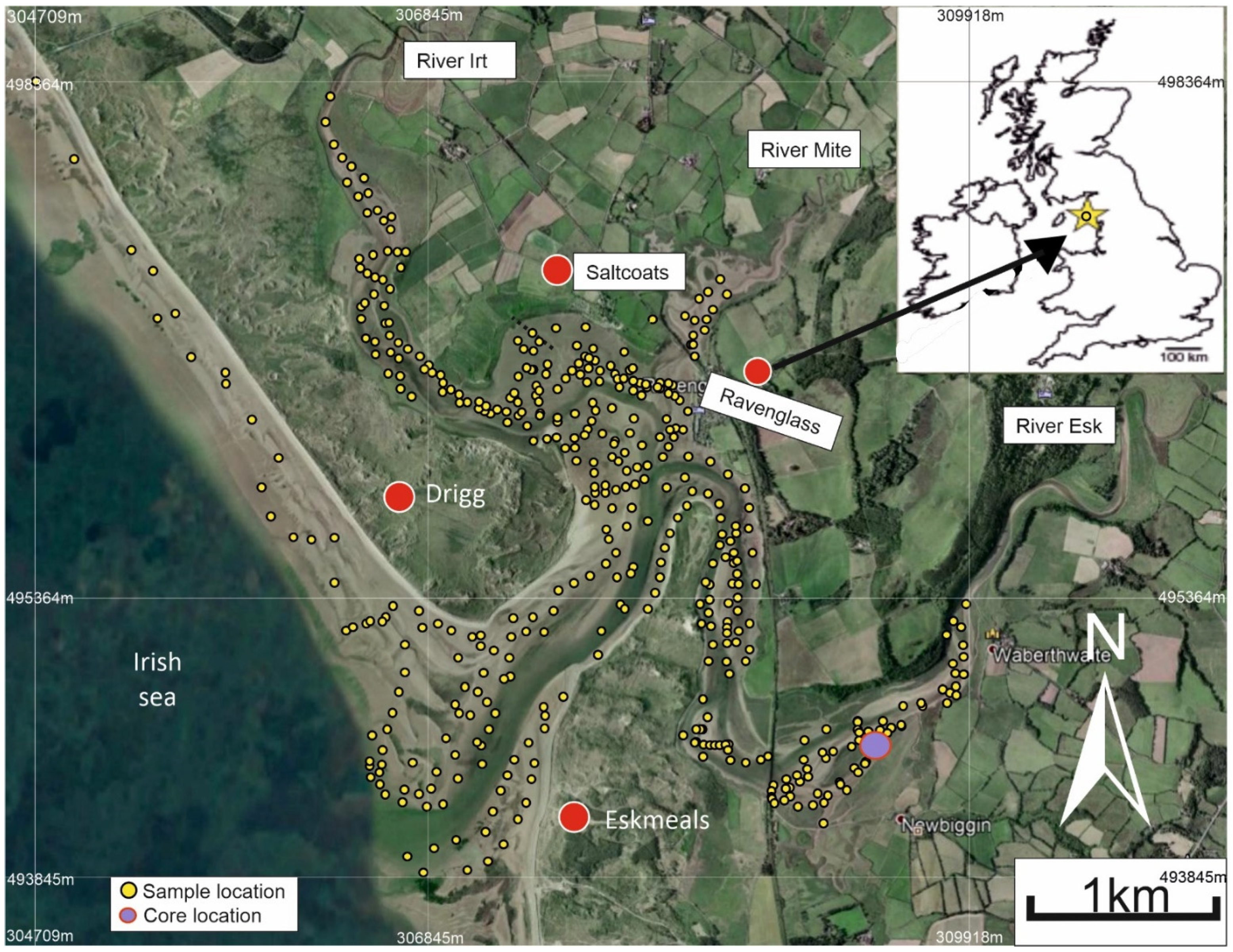
2. Study Area: The Ravenglass Estuary

The Ravenglass Estuary is situated on the west coast of Cumbria in northwest England, UK and covers an area of approximately 5.6 km2 (Figure 1). The estuary is macro-tidal with a maximum recorded tidal range of ~7.55 m; up to approximately 86% of the area of the estuary is exposed at low tide [45,46,47,48,49,53,54]. The estuary extends eastwards up to the tidal reaches of the Rivers Mite, Irt and Esk and is connected to the Irish Sea through a single tidal inlet, 500 m in width, that flows between two, dune-topped coastal spits (Drigg and Eskmeals spits). The coastal spits shelter the estuary from wave-action, but the estuary has strong tidal currents as result of the macro-tidal regime. The Rivers Mite, Irt and Esk have average flow rates of 0.4, 3.4, and 4.2 m3s−1, respectively [54]. Kelly, Emptage [55] classified the estuary as tide- and wave-dominated and ‘dual-funnelled’ and described the shallow bathymetry which causes frictional effects and promotes strong tidal-asymmetry, with a longer outward ebb tidal-flow than inward flood tidal-flow. The impact of anthropogenic activities on the Ravenglass Estuary is relatively low because the surrounding environment is sparsely populated. However, the construction of the Esk and Mite railway bridges in 1868 led to expansion of salt marsh due to added localised sheltering from tidal currents [56].
The inner estuary contains brackish water and has moderate fluvial influences from the Rivers Irt, and Esk (Figure 1 and Figure 2). The central part of the estuary, containing Saltcoats tidal flat, has mixed energy (fluvial, tide and wave-influenced) with near-seawater salinity (Figure 1 and Figure 2). The outer estuary is dominated by seawater with wave and/or tidal currents; this covers the main tidal channel, estuary mouth and the foreshore (Figure 1 and Figure 2).
Sedimentary deposits are fed into the estuary via the Rivers Mite, Irt and Esk. The sediments drain from a range of different bedrock types and Quaternary drift-deposits. The hinterland geology is comprised of Ordovician Borrowdale Volcanic Group (BVG), Devonian Eskdale Granite and Cambrian Skiddaw Group slate; a small area of Triassic Sherwood Sandstone Group, at the west of the drainage area, is largely covered by drift. Quaternary drift-deposits are dominated by glacial diamicton, peat, and glacial-fluvial-lacustrine deposits [47,48,49,57]. Eskdale Granite-sourced sediment was transported into the estuary via the River Esk, while BVG andesite-sourced sediment was transported into the estuary via the River Irt [47,48,49,50]. The post-glacial, Holocene, record represents approximately 10,000 years of deposition [58]. The estuary has been extensively studied in terms of sedimentary systems and processes, detrital clay mineralogy and distribution, detrital clay coat origin, mineralogy and distribution [45,46,47,48,49,50,51] and so represents an ideal field site to answer the research questions set out in the introduction.

3. Samples and Methods

3.1. Field-Based Mapping and Samples Collection

Based on geomorphological mapping criteria, together with the use of aerial imagery and grain size analysis, we have mapped eleven sub-depositional environments across the estuary (Figure 2). The sub-depositional environments are gravel beds, vegetated surfaces, barrier spits, tidal flats (sub-divided into mud flat, mixed flat and sand flat), tidal bars, tidal inlet, backshore, foreshore, ebb-tidal delta (Figure 2). The subdivision of tidal flats was based laboratory-derived sand percentages, modified from a scheme initially proposed by Brockamp and Zuther [59], where: 90–100% sand is sand flat, 50–90% sand is mixed flat, and 15–50% sand is mud flat.
We sampled surface sediment (from <2 cm below the surface) from 497 sites covering the entire estuary and the coastal portion of the system (Figure 1). Sediment samples were placed in airtight plastic bags in the field and dried in the laboratory prior to geochemical pXRF analysis.

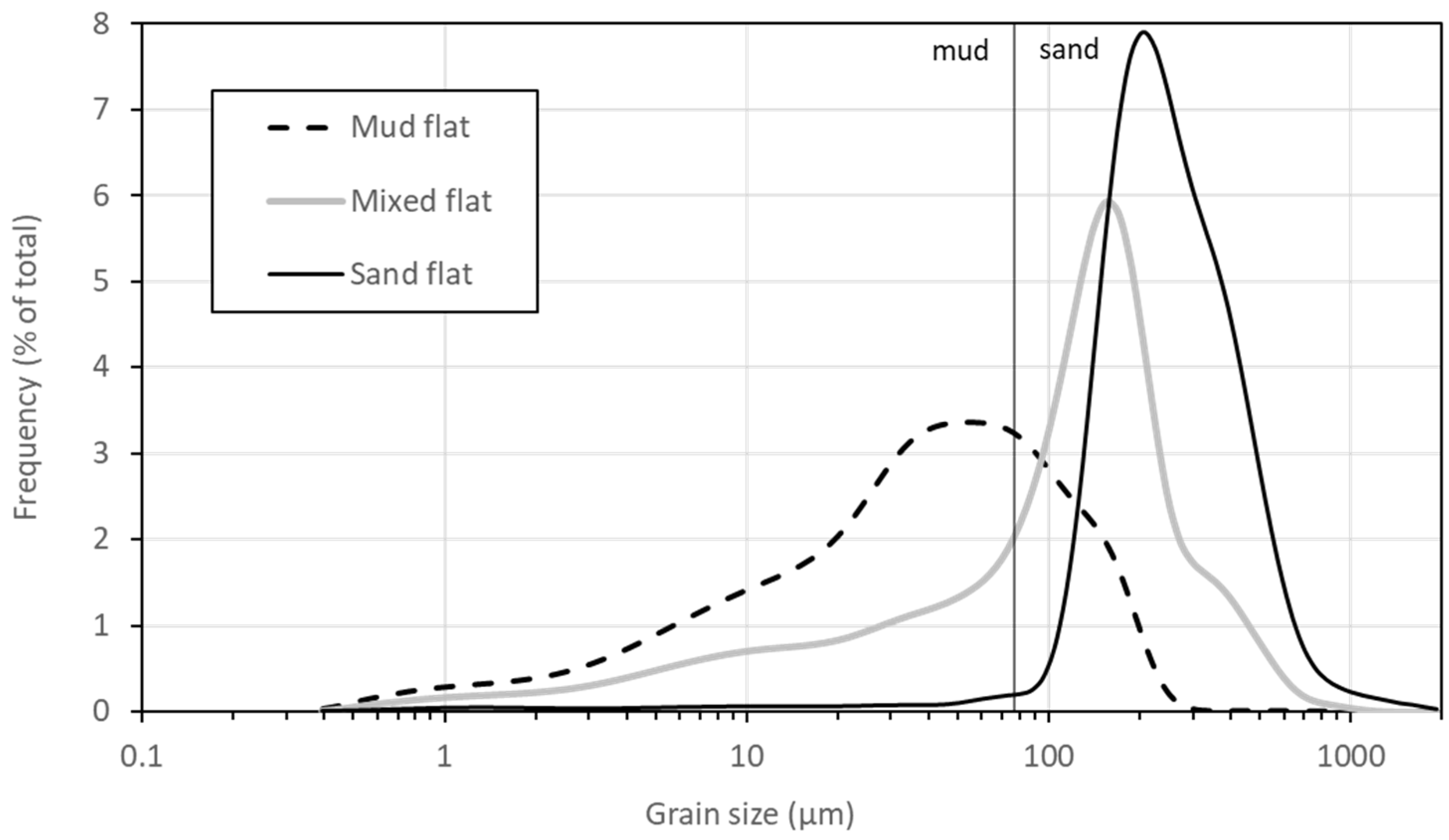
3.2. Grain Size Analysis

Grain size analysis was undertaken solely to differentiate the sediments of the tidal flats into mud-, mixed- and sand-flat sub-depositional environments. Grains <2 mm were separated from the sample using a sieve and then this fraction was analysed for grain size distribution using laser particle size analysis (LPSA) with a Beckman Coulter LS13 320 Counter. Organic matter was removed using established laboratory procedures for sample digestion [50]. A small amount of Calgon was added to convert the dried sediment into a paste for mixing and homogenisation, prior to analysis [52]. The LPSA data were analysed using GRADISTAT© to define grain size parameters of the sediment.

3.3. Multi-Element Analyses Using Handheld Niton +XL3t GOLDD pXRF Spectrometer

All sediment samples from Ravenglass were analysed using a handheld Thermo Scientific Niton +XL3t GOLDD XRF spectrometer (pXRF) to measure the abundance of major, minor and trace elements. The pXRF equipment is a self-contained, energy dispersive XRF spectrometer with a variable intensity energy source (6–50 kV, 0–200 μA) Ag anode X-ray tube. It is equipped with a factory-calibrated, GOLDD (Geometrically Optimised Large area Drift Detector) detection system, optimised by the manufacturer for low detection limits, and high-precision measurements of more than 40 elements. Sediment samples were prepared by air drying whole-sediment samples in a 50 mm Petri dishes which was then placed 2 mm from the pXRF detector. Problems of horizontal and vertical heterogeneity of the sample, variable moisture and surface roughness, associated with core-based, “point and shoot” pXRF studies [30,60,61,62] have here been avoided [63].
Despite concentrations for 40 elements being reported by the pXRF, only 12 elements were present in all samples. These elements are Al, Si, K, Ca, Ti, Fe, Mn, Rb, Sr, Zr, Ba and Cs. Other elements were variably present at concentrations above the element-specific detection limit, but these elements, with values below detection in some samples, could not easily be incorporated into any scheme to interrogate the relationship between composition and the sub-depositional environment.
The reported limit of detections of the instrument for Al, K, Ca, Ti, Fe, Mn, Rb, Sr, Zr, Ba and Cs are listed in Table 1. The instrument’s high precision and accuracy was validated by replicating the pXRF analysis, on a single sample 30 times; the average and standard deviation of Al, K, Ca, Ti, Fe, Mn, Rb, Sr, Zr, Ba and Cs are listed in Table 1. Each analysis was conducted, for 150 s, in “Test All GEO” mode; this combines mining and soil modes which thus permits the determination of major and trace elements. The optimum analysis time of 150 s was selected by repeating analysis of one sample for different replicate durations in order to identify when there was no significant improvement in the reported uncertainty.

3.4. Spatial Mapping

Spatial distribution maps of elements and element indices were generated using ArcGIS software, via an inverse distance weighted (IDW) interpolation function. The IDW approach has lower mean prediction errors and higher correlations between predicted and measured values than other mapping tools [64]. IDW was also selected to avoid the automatic generation of physically-meaningless negative concentrations, such as are produced by spline-based interpolation methods, and to avoid the formation of valleys or ridges [65]. A polyline in ArcGIS was drawn down the long axes of the Drigg and Eskmeals spits, to separate the marine data from estuarine data when performing the interpolations [48].

3.5. Statistical Multivariate Analysis

Multivariate statistical techniques are powerful tools commonly used to investigate variability in large datasets [66,67,68,69]. Although we will display concentration maps of elements, there is a risk that all we will display is greater or smaller amounts of element dilution by SiO2 due to variable quantities of the dominant mineral, quartz. To evaluate the more meaningful relative abundance of elements, we have calculated a range of indices (e.g., X/(X+Y)) and mapped these values. We choose not to use ratios as they vary from infinitely large to infinitely small and multi-order of magnitude ranges are difficult to map and present problems for machine learning approaches. We have avoided indices of elements that are strongly autocorrelated due to their geochemical similarity (e.g., K and Rb; Ca and Sr; Fe and Mn). We produced a correlogram (available on request) using R statistical software to identify the presence of strong element correlations (e.g., K and Rb) and to identify elements that have the greatest non-correlation and so reveal most about the geochemical variability of the estuary. The indices we have employed are: K/(K + Si), K/(K + Al), K/(K + Ca), K/(K + Ti), K/(K + Mn), K/(K + Sr), Sr/(Sr + Rb), Ca/(Ca + Fe), and Mn/(Mn + Sr); maps and boxplots of these indices will be presented. These elemental indices were selected as they were the ones that subsequent machine learning (recursive partitioning) employed to differentiate sub-depositional environments (see later text in Section 5.5). However, we have also mapped the spatial distributions of Fe/(Fe+Ti), K/K + Fe) and Al/(Al + Fe), because Fe is of relevance to the understanding of Fe-clay minerals in the estuary.

3.6. ANOVA and Tukey’s Post Hoc Test

Analysis of variance (ANOVA) tests were used in R statistical software [70], to investigate the statistical significance of geochemical differences between various pairs of sub-depositional environments. Following ANOVA, Tukey’s post hoc honestly significant difference (HSD) test was then employed, using R statistical software [70], to determine which individual depositional environments were statistically different from one another as a function of elemental indices. The difference between each pair, for each elemental index, is defined as being significant if the “p” value is less than 0.05 [70,71].

3.7. Boxplots and Classification Trees

Univariate analysis of geochemical indices, split by the sub-depositional environment, was undertaken using boxplots produced using ggplot2 in RStudio [72]. The Recursive Partitioning and Regression Tree (RPART) package [73], available in R statistical software [70], was used to classify the sub-depositional environments (categorical data) using sediment geochemical signatures (continuous data). The RPART routine allows the development of a classification tree by using one or more variable (in this case, elemental indices) to find the optimum splits of the dataset, into different categories (e.g., sub-depositional environment) [52].

3.8. Holocene Cores

A sediment core was drilled through the Holocene succession in the tidal bar sub-depositional environment in the Esk arm of the inner Ravenglass Estuary, under tender by Geotechnical Engineering Ltd. (GEL) [58]. The drilled core was retrieved in a series of 12 cm diameter, 1 m length, semi-rigid plastic liners for protection and easy transport. Each 1 m segment of the sediment core was sliced and photographed wet and air-dried for extensive study and subsequent analysis at the University of Liverpool. The core description involved detailed sedimentary logging of each core segment, at a scale of 1:5, and lithofacies were characterised in terms grain size, colour, sedimentary structures, bed thickness, presence of roots and shell fragments, bioturbation extent and type. The core was sampled at 5 cm intervals for pXRF and LPSA analyses, using techniques described above.

4. Results

Here, we present details of the distributions of sub-depositional environments in the Ravenglass Estuary and the absolute and relative distribution of elements.

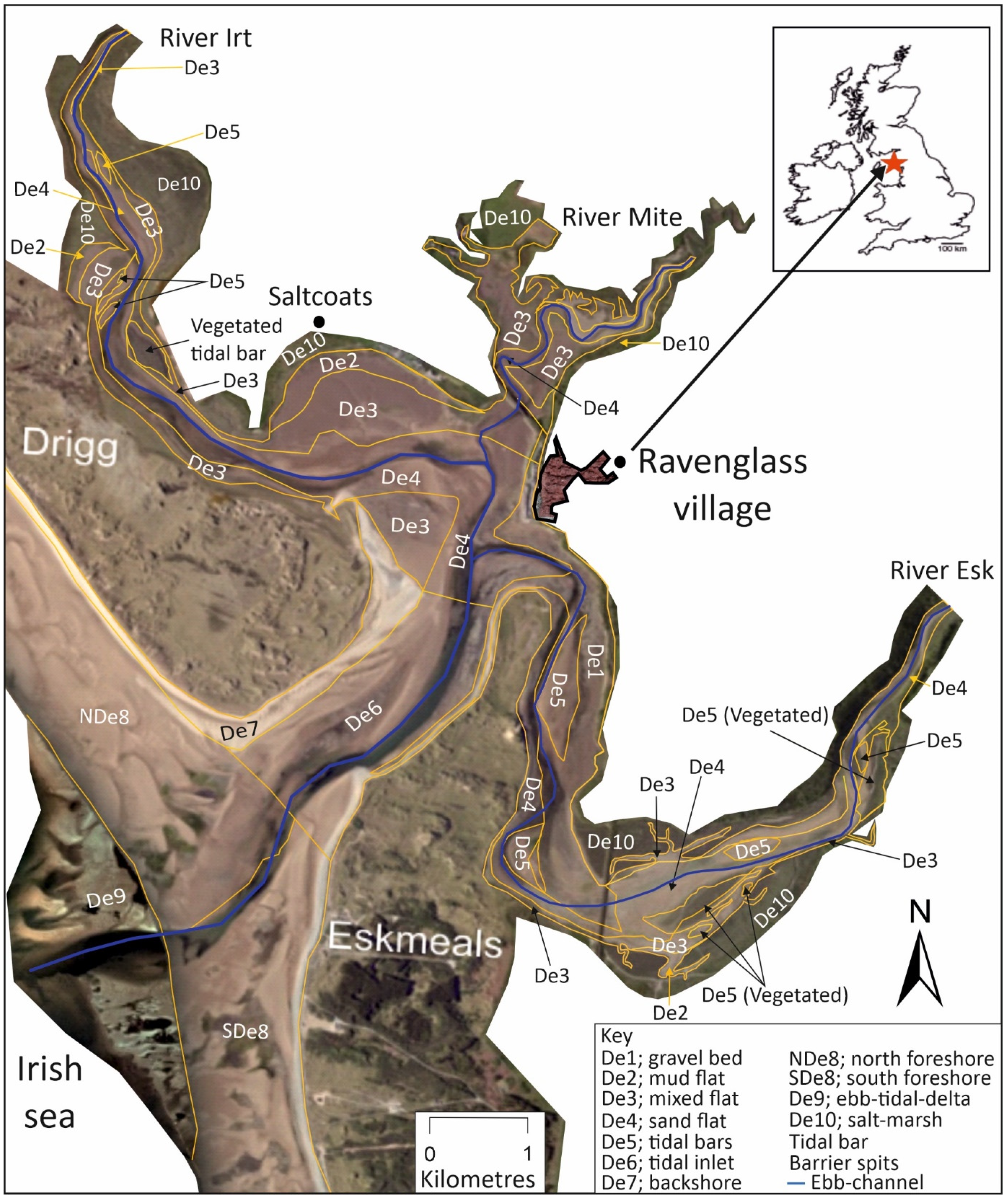
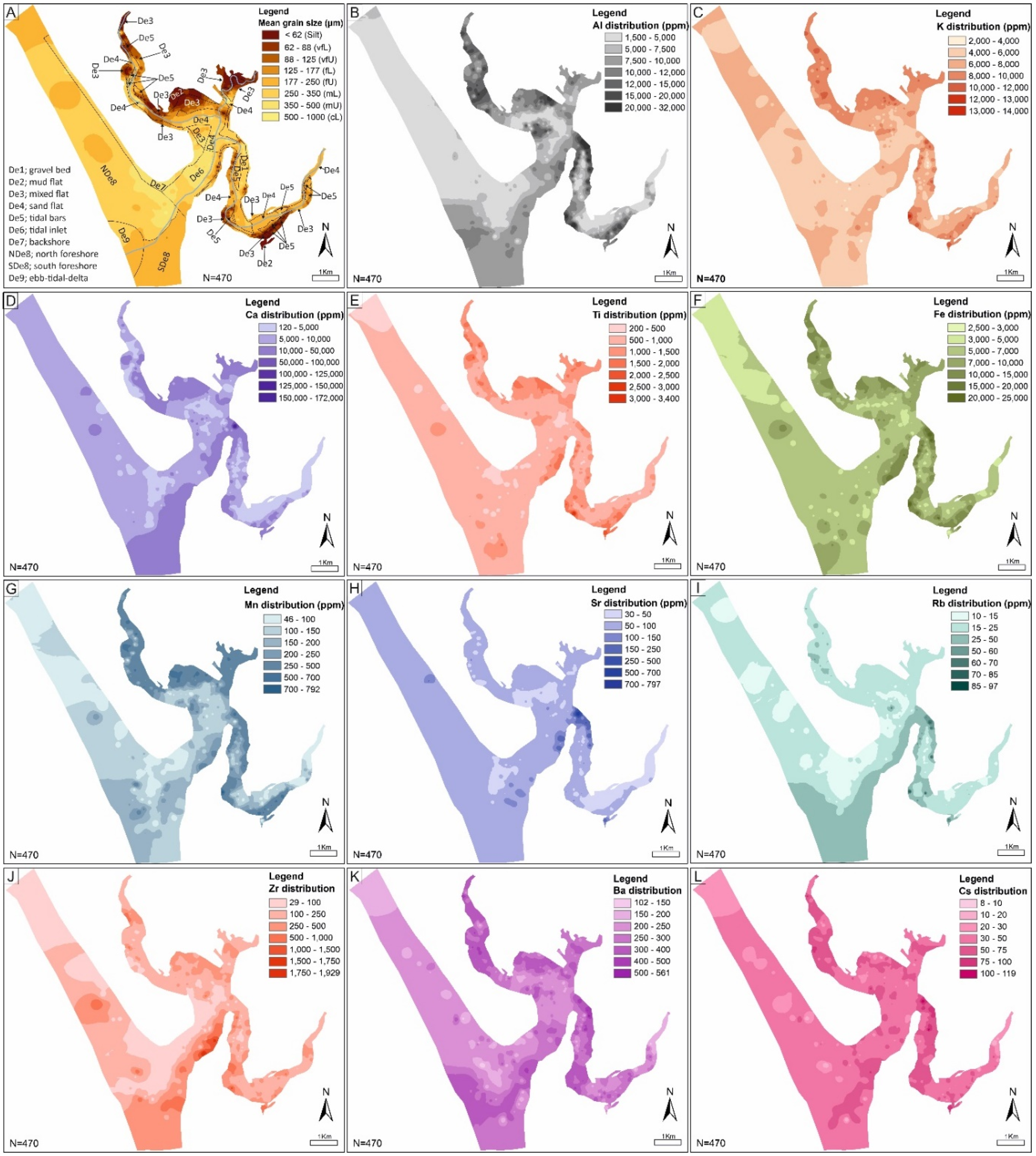
4.1. Sub-Depositional Environments Present across the Estuary

The sub-depositional environments identified and mapped (Figure 2) across the Ravenglass Estuary are gravel beds (De1), tidal flats (sub-divided into mud flats, De2, mixed flats, De3, and sand flats, De4), tidal bars (De5), tidal inlet (De6), backshore (De7), foreshore (De8), ebb-tidal delta (De9), and salt marsh (De10). The subdivision of tidal flats was based on laboratory-derived laser particle size analysis data, with average grain size distribution curves for the mud, mixed and sand flats illustrated in Figure 3.
The inner estuary comprises: (a) gravel beds (De1), which are locally distributed in the lower part of the Esk and Irt arms of the estuary and are dominated by a loose aggregate of rock fragments; (b) salt marsh (De10), which is present in the Esk and Irt arms of the estuary and is dominated by salt-tolerant plants; (c) tidal bars (De5), which are sand bars present in the intertidal zone and which usually have a long axis oriented parallel to the direction of the main current; (d) sand flats (De4), which are intertidal flats bordering the main channel; (e) mixed flats (De3), which are sandwiched between sand mud flats; (f) mud flats (De2), which are furthest away from the main channel (Figure 2).
The central estuary includes extensive tidal flats and comprises: (a) sand flats (De4); (b) mixed flats (De3); (c) mud flats (De2); and (d) salt marsh (De10).
The outer estuary contains: (a) the main tidal inlet (De6) that cuts between the Eskmeals and Drigg barrier spits; (b) foreshore (De8), which is the part of the beach, that lies between the backshore and the mean-low-water line; and (c) backshore (De7), which is situated above the mean-low-water line and can be inundated during spring tides and storm events. The foreshore has been split into two portions, north and south of the main channel (becoming NDe8 and SDe8), as these areas have texturally (and, as it turns out, geochemically) distinct sediment. NDe8 is coarser grained than SDe8.

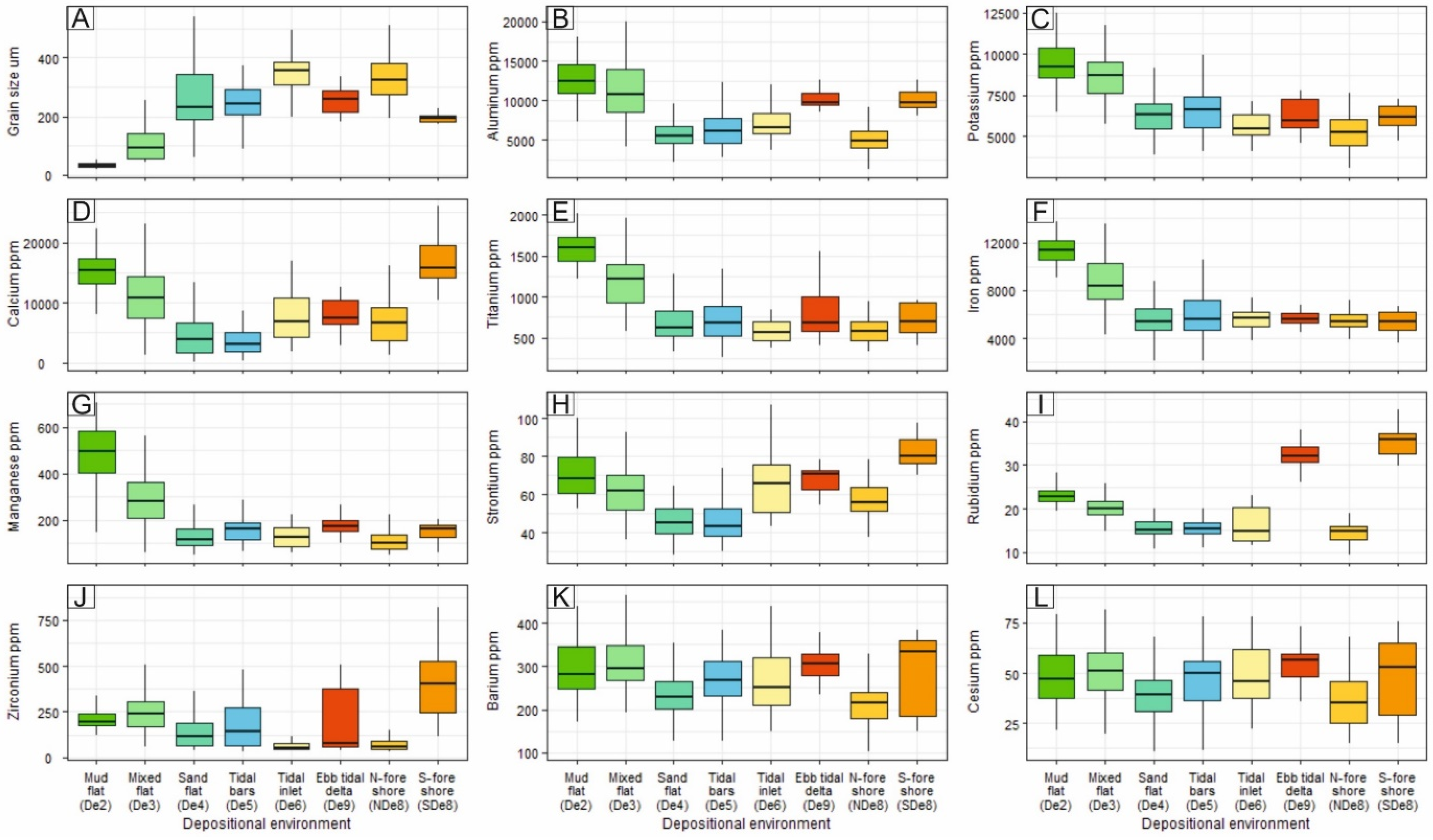
4.2. Element Concentrations in the Ravenglass Estuary

The number of samples from each depositional environment that are above the detection limit is shown in Table 2. A summary of elements with their minimum reported values is presented in Table 3, where, for elements that have many samples below detection, the minimum reported value effectively represents the detection limit in Ravenglass surface sediments.
The elements present in Ravenglass surface sediments include major elements typically present in all samples: Al, Si, K, Ca, Fe, S and Ti. Minor elements, here defined as between 100 and 1000 ppm, include Cl, Mn, Rb, Zr, and Ba. These minor elements were detected in all samples from all the different sub-environments. Trace elements, here defined as <100 ppm, present in Ravenglass sediments include P, Sc, V, Cr, Ni, Cu, Zn, As, Sr, Nb, Pd, Ag, Sn, Sb, Te, Cs, Hg, Pb, Bi, Th and U. These trace elements were detected in small to negligible quantities in some samples but were below detection in many samples (Table 3 and Table 4).
Maps of the distribution of elemental concentrations of major, minor and trace elements have been plotted to assess the distribution in relation to geographic location and sub-depositional environments. Maps of grain size, and the concentrations of Al, K, Ca, Ti, Fe, Mn, Sr, Rb, Zr, Ba and Cs are shown in Figure 4. The map showing grain size distribution across the estuary (Figure 4A) has had boundaries between sub-depositional environments from Figure 2 superimposed.
Grain size tends to increase down channel and decrease toward the margin of inner estuary and central basin (Figure 4A). The map of Al abundance (Figure 4B) has a marked similarity to the grain size map (Figure 4A). Aluminium is not homogeneously distributed between different sub-depositional environments (Figure 5B). Aluminium is present at elevated concentrations in the mud and mix flat environments (De2 and De3); Al is present at intermediate concentrations in the ebb-tidal delta and southern foreshore (De9, SDe8); Al is present at relatively low concentrations in the sand-dominated sand flat, tidal bar, tidal channel and northern foreshore environments (De4, De5, De6 and NDe8).
The spatial distributions of K and Fe are heterogeneous and have some similar features (Figure 4C,F). Potassium abundance decreases progressively toward the open sea and tends to be highest in tidal flat sediments; there is a relative increase in K abundance in the upper reaches of the northern foreshore (Figure 4C). Iron and Ti abundances also have some similarities as they have highest concentrations in tidal flats, tidal bars, and in <2 mm sediment from gravel beds. Overall, the relative abundance of Fe and Ti decreases progressively toward the open sea (Figure 4E,F). Potassium, Fe and Ti are unevenly distributed between different sub-depositional environments (Figure 5C,E,F). Potassium, Fe and Ti are present at elevated concentrations in the mud and mix flat environments (De2 and De3); they are present at relatively lower concentrations in all remaining sub-depositional environments (De4, De5, De6, NDe8, SDe8 and De9).
The concentration of Ca in the Ravenglass Estuary sediment is heterogeneous; across the southern foreshore and tidal inlet and some pockets within the inner estuary and central basin, there is significant Ca enrichment (>10,000 ppm) (Figure 4D). Some of the highest concentrations of Ca (>100,000) are found in <2 mm sediment from gravel beds located at the boundary with the central basin and the upper Esk arm (Figure 4D). Boxplots show that calcium is not homogeneously distributed between different sub-depositional environments (Figure 5D). Calcium is present at elevated concentrations in the mud and mix flat environments and in the southern foreshore (De2, De3 and SDe8); calcium is present at intermediate concentrations in the tidal inlet, ebb-tidal delta, and northern foreshore (De6, De9, NDe8); calcium is present at relatively low concentrations in the sand-dominated sand flat and tidal bar environments (De4, De5).
The abundance of Mn is highest (200 to 700 ppm) in the upper and lower reaches of the Irt arm of the estuary, in the mud and mixed flats of the central basin and in the finer-grained parts of the upper and lower Esk arm (Figure 4G). Manganese is heterogeneous across the outer estuary with abundance broadly decreasing progressively toward the open sea. Manganese is unevenly distributed between different sub-depositional environments (Figure 5G). Manganese is present at elevated concentrations in the mud and mix flat environments (De2 and De3); manganese is present at relatively low concentrations in all remaining sub-depositional environments (De4, De5, De6, NDe8, SDe8 and De9).
Strontium is mostly a trace element with concentrations <100 ppm across much of the estuary, but the <2 mm sediment from gravel beds has unusually high Sr concentrations (>700 ppm) (Figure 4H). Strontium is heterogeneously distributed between different sub-depositional environments (Figure 5H); the sub-environment distribution of strontium closely matches the distribution of calcium.
Rubidium is a trace element with relatively low concentration (<15 ppm) across the estuary except in the southern foreshore, part of the tidal inlet, gravel beds and margins of the upper Esk estuary, where the concentrations are highest and reach up to 70 ppm (Figure 4I). Rubidium is not uniformly distributed between different sub-depositional environments (Figure 5I). Rubidium has the highest concentration in the ebb-tidal delta and southern foreshore (De9, SDe8); rubidium is present at intermediate concentrations in the mud and mixed flats (De2 and De3) and low concentrations in all other sub-depositional environments.
Zirconium varies from <100 to nearly 2000 ppm (Figure 4J). The most noteworthy aspects of the distribution of Zr are the high concentration along the southern part of the tidal inlet and southern foreshore and the low concentration along the northern part of the tidal inlet and northern foreshore. Like all other elements, zirconium is heterogeneously distributed between different sub-depositional environments (Figure 5J). Zirconium is present at the highest concentrations in the southern foreshore (SDe8).
Barium concentrations range from approximately 160 to 540 ppm (Figure 4K). Barium is present at highest concentration in parts of the Esk and Irt arms of the estuary, along the southern side of the tidal inlet and in the ebb-tidal delta. Barium concentrations do not seem to show any systematic pattern with the sub-environments of deposition (Figure 5K).
Caesium has a modal concentration of 35 to 50 ppm (Figure 4L). Caesium concentrations are slightly higher in the lower part of the Esk estuary, the upper part of the Irt estuary and along part of the southern side of the tidal inlet. Like barium, caesium concentrations (Figure 5L) do not seem to show any systematic pattern for the sub-environments of deposition.
We have here not mapped the distribution of Cl as it is wholly linked to halite precipitation from seawater and may reflect estuary water composition rather than sediment composition. Similarly, we have not mapped the distribution of sulphur as it is present as a sulphate mineral in the sediment and will be an evaporite mineral, like halite, or linked to Fe-sulphide oxidation.

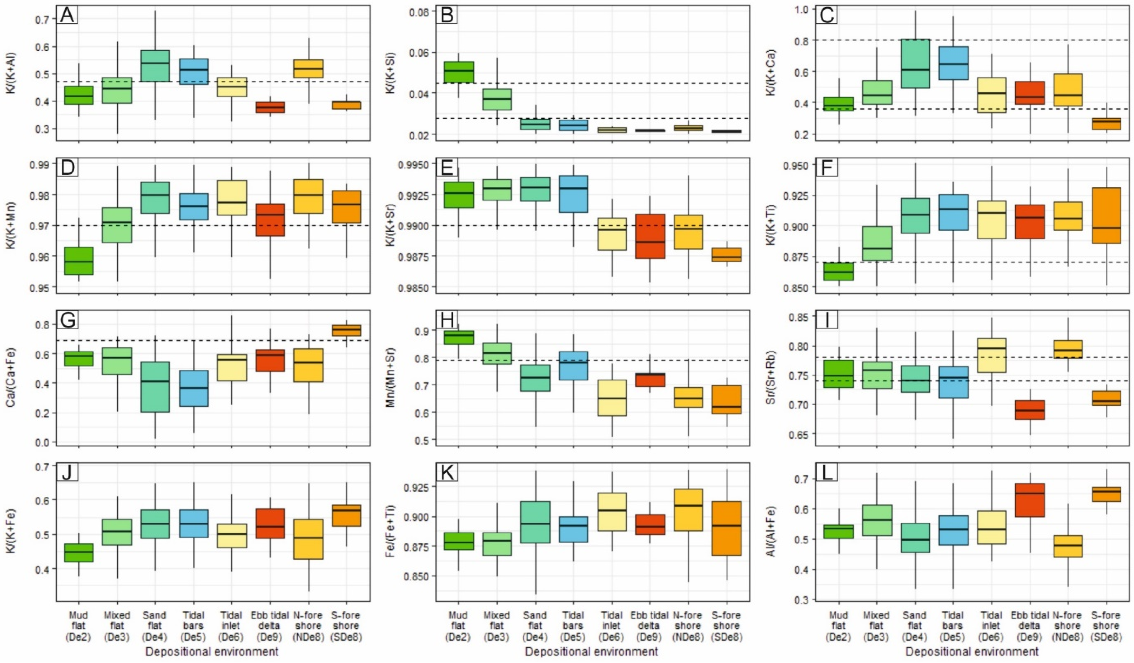
4.3. Relative Element Concentrations
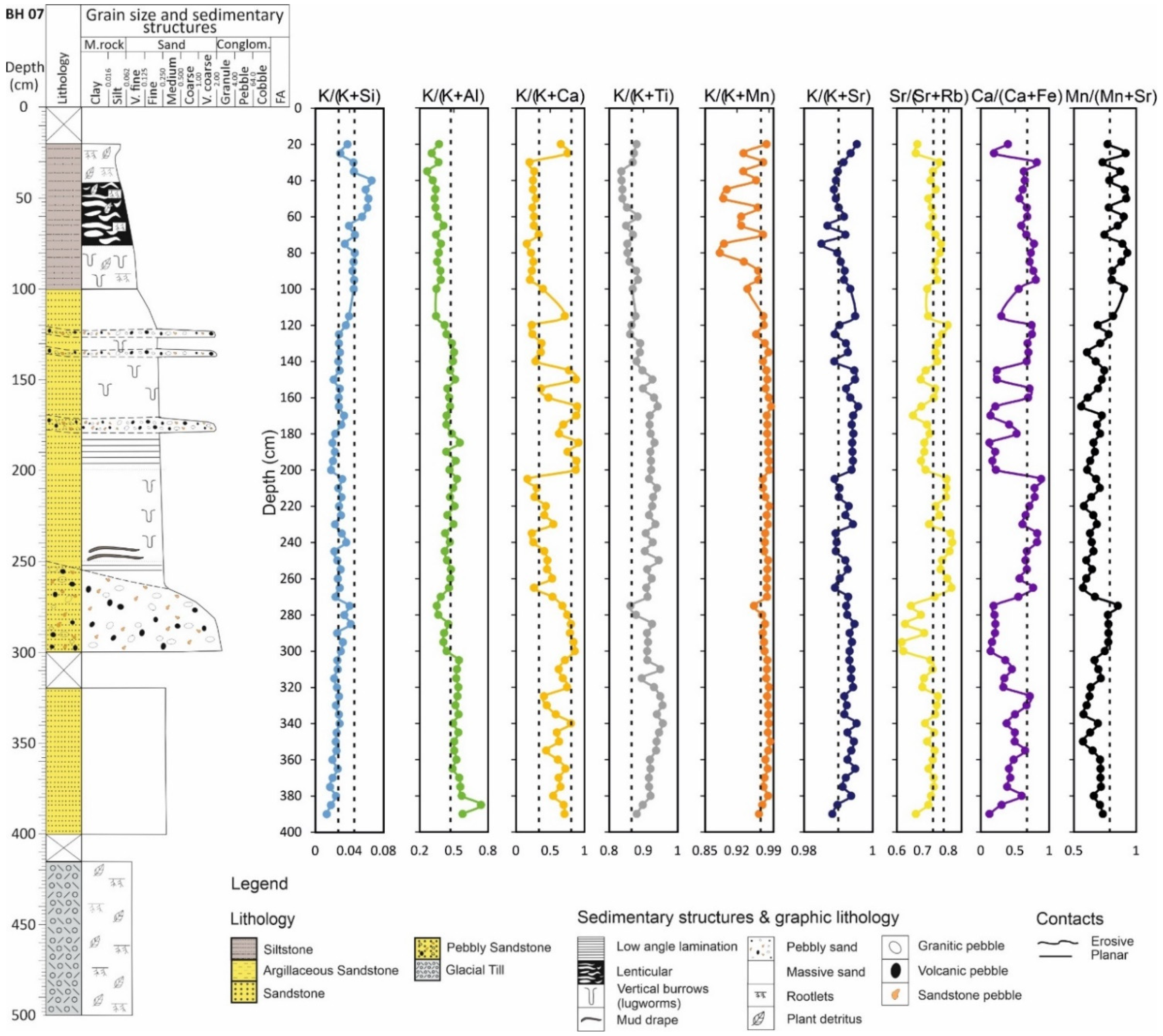
Maps displaying surface sediment characteristics, such as elemental concentration, are generally considered to be an important tool for sediment analysis [74]. However, elemental concentrations in quartz-rich sediment will be strongly influenced by the diluting effect of quartz [48], as this mineral is effectively pure SiO2 and contains next to no trace elements. All element concentration maps (Figure 4B–H) will be strongly influenced by variable depletion and enrichment of quartz. However, the observation that not all the elemental concentration maps are identical (Figure 4B–H) suggests that there are meaningful differences in the sediment composition that are not due to variable depletion and enrichment of quartz.
The element index maps show that the spatial distributions of K/(K + Al) and K/(K + Mn) have some similar features (Figure 6A,D). The data from the index maps are summarised as a series of boxplots, displayed in Figure 7. K/(K + Al) and K/(K + Mn) increase progressively toward the open sea and tend to be low in tidal flat sediments (Figure 6A,D and Figure 7A,D). K/(K + Al) in the foreshore and tidal inlet is relatively lower in the north side than the south side. K/(K + Mn) has variable distribution in the upper reaches of both Esk and Irt arms, and in the outer estuary (Figure 6D).
K/(K + Si), K/(K + Sr), and Mn/(Mn + Sr) tend to decrease progressively toward the open sea and are highest in the inner estuary and central basin (Figure 6B,E,H and Figure 7B,E,H). Sr/(Sr + Rb) has a narrow range of values, with most falling between 0.677 and 0.816, except along the upper reaches of both the Esk and Irt arms of the estuary, and in the ebb-tidal delta and south foreshore where it is low (Figure 6I).
K/(K + Ca) and K/(K + Ti) are quite variable across the study area (Figure 6C,G,F and Figure 7C,G,F). K/(K + Ti) is low in a range of areas including the southern foreshore, ebb-tidal delta, the southern part of the main channel and the mixed and mud flats of the central basin and a few other sporadic localities (Figure 6F). K/(K + Ca) is highest in both the upper reaches of the Irt and Esk arms of the estuary; it is intermediate in the gravel bed, the middle part of the central basin, and the northern part of the tidal inlet and into the northern foreshore (Figure 6C).
Indices related to Fe concentration are variable across the estuary. The Ca/(Ca + Fe) index is lowest in both the upper reaches of the Irt and Esk arms of the estuary and it is intermediate in the mixed and mud flats of the central basin and much of the northern and southern foreshores (Figure 6G and Figure 7G). The southern foreshore and parts of the southern side of the tidal inlet have the highest Ca/(Ca + Fe) index values (Figure 6G). K/(K + Fe), related to the Fe/K index used for clastic sedimentary rock geochemical classification by [75], shows that most values fall into an intermediate category (Figure 6J and Figure 7J). The highest values are in the tidal bars of the Esk and Irt and at some localities within the foreshore and tidal inlet. Fe/(Fe+Ti), where both elements are mafic indicators, is highest in the middle part of the system, from the uppermost Esk arm through the northern part of the main channel (Figure 6K and Figure 7K). This index is lowest in the southern foreshore, ebb-tidal delta, and mixed and mud flats of the Esk and Irt inner estuaries. Al/(Al + Fe) is lower in the Esk arm than the Irt arm of the estuary; it is also low in parts of the northern foreshore (Figure 6L). Al/(Al + Fe) is highest in the southern foreshore, the ebb-tidal delta and parts of the Irt arm of the estuary (Figure 6L).

4.4. Holocene Cores

Based on the sedimentary log of the geotechnical core [58], mud and sand are the dominant lithologies in the tidal bar in the Esk arm of the estuary (Figure 8). This sand-dominated core has a narrow grain size range. The core was drilled into a vegetated tidal bar (fresh marsh) sub-depositional environment at the surface; the uppermost part down to 100 cm in depth is dominated by mud to very fine sand (Figure 8). Below this depth, most of the sediment is composed of different units of medium- and coarse-grained sand that may represent mixed fluvial-tidal deposits [58]. The specific sedimentary sub-depositional environments in this core could not have been automatically predicted as there is a range of grains sizes (gravel beds through to mud-dominated sediment) not typical of vegetated tidal bars. The Holocene core was analysed using the pXRF spectrometer, and the nine key indices used to classify the sediment (and see Figure 6 and Figure 7 and Section 5.5) are shown with critical cut-off values marked by dashed lines.

5. Discussion

The primary objective of this study was to determine the ability of pXRF data to discriminate sedimentary environment in an estuarine setting. To ascertain how elemental data can be used to predict sub-depositional environments, parameters such as sediment source areas, and the statistical relationship between element concentrations and sub-environment, will be evaluated and discussed.

5.1. Elemental Distribution in the Ravenglass Estuary

One of the aims of this research was to understand the controls on the distribution of elements across an entire estuarine system. This is of interest to clastic sedimentary geologists, especially those who work with rock properties, because elemental distribution reflects, and potentially controls, mineral distribution via clay synthesis, Fe-reduction and silica precipitation [50,76,77,78,79].
The distributions of Al, K, Ca, Ti, Fe, Mn, Sr, and Rb, as well as Zr, Ba and Cs, in the sediment of the Ravenglass Estuary vary greatly with some apparent links to sub-depositional environment and geographic location (Figure 4). For example, Al and K display similar maps of concentration patterns (Figure 4B,C). Aluminium and K are present at the highest concentrations in the finest-grained sediments of the mud and mixed flat sediment (De2 and De3) and are present at the lowest concentrations in coarsest-grained sediments of the northern foreshore and parts of the tidal inlet (De6 and NDe8) (Figure 4A–C and Figure 5A–C). Aluminium sits predominantly in the detrital minerals K-feldspar, muscovite, plagioclase, and in the dominant clay mineral, illite, with lesser quantities of detrital biotite and chlorite and weathering-related kaolinite [48]. Potassium sits predominantly in K-feldspar, muscovite, and illite with lesser quantities in biotite [48]. The distribution patterns of Al and K are almost certainly controlled by illite clay distribution as they are present at the highest concentrations in the finest-grained sediment (Figure 4A–C). Conversely, if Al and K were largely controlled by K-feldspar distribution, then the highest concentrations of these elements would be in the coarser sedimentary sub-depositional environments. The dominant role of weathering-related illite in controlling Al and K distribution reveals the important role of chemical weathering in the hinterland. Rubidium has similar geochemical properties to K, in terms of ionic radius and charge [80], and the two elements seem to have broadly similar distributions in the estuary (Figure 4I), although the concentration of K is high in the mixed and mud flats (Figure 4C) whereas the concentration of Rb is relatively low, possibly indicating that Rb is partly controlled by variable K-feldspar as well as illite abundance (given that mixed and mud flats are the finest-grained sediment in the estuary (Figure 4A).
Iron, Mn and Ti concentrations display some similarities in terms of their mapped distributions at Ravenglass (Figure 4E–G). Iron, Mn and Ti are present at the highest concentrations in the finest-grained sediments of the mud and mixed flat sediment (De2 and De3) and are present at the lowest concentrations in coarsest-grained sediments of the foreshore, tidal inlet, tidal bar (De5, De6, SDe8, NDe8, and De9) (Figure 4A,E–G and Figure 5E–G). Iron and Mn have similar geochemical properties, as they can have a similar ionic radius and charge (when divalent) but they both have variable oxidation states. Iron and Mn probably exist in the Ravenglass sediment in a combination of divalent ions within detrital lithic grains and minerals (e.g., chlorite and biotite) [48] and in higher valence states in weathering products such as hydroxides [51]. Iron is preferentially concentrated in the upper reaches of the Ravenglass Estuary (Figure 4F), confirming that fluvially-transported iron is trapped at the site of mixing between river water and seawater [81]. In contrast, Ti can sit in ilmenite and rutile (and other oxides) or as a trace element in mica minerals. In the Ravenglass Estuary surface sediments, the rutile concentration is approximately 0.40% in mud and mixed flats and approximately 0.10% in the sand-dominated environments [82]. The increase in Ti in the finest-grained sediments is therefore likely to be due to rutile as well as mica minerals (illite, muscovite and biotite) (Figure 4A,E).
Calcium displays a strongly variable distribution (Figure 4D). The concentration of calcium closely matches the distribution of CaCO3 (calcite and aragonite) [48]. CaCO3 is largely found as bioclastic material, including large (10 cm) shells in the gravel beds on the lower Esk Estuary and the southern side of the tidal inlet. Strontium has similar geochemical properties to calcium and is present in carbonate minerals, especially aragonite; Sr can substitute for Ca in carbonates [83]. However, the relationship between Ca and Sr maps is not especially strong (Figure 4D,H). Strontium seems to display a weak relationship with Ravenglass sub-depositional environments but there are some pockets of local enrichment, especially in gravel-rich sediment deposits, potentially due to their present in lithic fragments [84,85], and shell fragments possibly due to the Sr–Ca association
Zirconium is probably only present in the mineral zircon. The distribution of Zr reveals the distribution of zircon (Figure 4J). The map of Zr (Figure 4J) seems to follow the inverse of the grain size map, with the lowest concentrations of Zr in the coarsest-grained sands (Figure 4A).
Barium might be present, substituting for K, in detrital K-feldspar or possibly in barite. Caesium may also substitute for K in micas and feldspars. Barium and Cs have similarly bland distribution maps (Figure 4K,L), with most values varying tightly about the modal value, with the lowest concentrations in the coarsest-grained sands (Figure 4A). Variable dilution by quartz may be responsible for much of the variation in Zr, Ba and Cs.

5.2. Relationship between Element Indices and Sub-Depositional Environment

One of the problems with element concentration maps (Figure 4) is that they are strongly influenced by variable dilution by quartz and, perhaps to a lesser extent, calcite. Given that quartz has negligible trace elements, doubling the quantity of quartz would halve the concentration of a trace element, all other factors remaining the same. We therefore consider that relative element concentrations are more useful to understanding the relationship between sediment supply, weathering intensity, etc., and the sub-depositional environment [86]. Element indices have been analysed in terms of the sub-depositional environment as these will be useful for developing a quantitative classification tool.
K/(K + Al) is low in mud flats, ebb-tidal delta, and southern foreshore sub-environments (De2, De3, De9 and SDe8) (Figure 7A). It is highest in sand flat, tidal bar and northern foreshore sediment sub-environments (De4, De5 and NDe8). It has intermediate values in mixed flat and tidal inlet environments (De3 and De6). In these sediments, the K/(K + Al) index reflects the relative concentrations of K-feldspar, illite (and muscovite) and kaolinite (there is no gibbsite in these sediments); high values imply more K-feldspar, low values imply more kaolinite and illite.
K/(K + Si) simply reflects dilution by quartz of the collection of K-bearing minerals (K-feldspar, illite, muscovite and, to a lesser extent, biotite). This index is highest in the least quartz-rich, most fine-grained mud flat sediments (De2) (Figure 7B). It has consistently low values in the sand-rich sub-depositional environments (De4–De9) and an intermediate value in mixed flats (Figure 7B). Every other element indexed to silicon looks like Figure 7B, reflecting variable dilution by quartz; we have therefore chosen not to replicate such distributions as they all show the same pattern and do not help to further discern the sub-depositional environment. Silicon and its element indices seem to have minimal value to this study of estuarine sub-environments.
K/(K + Ca) is low in mud flats and southern foreshore sub-environments (De2, De3, SDe8) (Figure 7C). It is highest in sand flat and tidal bar sub-environments (De4, De5). It has intermediate values in mixed flat tidal inlet, northern foreshore, and ebb-tidal delta sub-environments (De3, De6, NDe8, De9). In these sediments, the K/(K + Ca) index reflects the relative concentrations of K-bearing K-feldspar, illite (and muscovite) compared to carbonate concentrations. As K concentration seems to be broadly consistent in all sand-dominated sub-environments (Figure 5C), the variation in K/(K + Ca) in these sandy sediments is largely due to variations in Ca (Figure 5D) and therefore CaCO3 minerals.
K/(K + Mn) is low in mud flats (De2) (Figure 7D). It is highest in sand flat, tidal bar, tidal inlet, and northern and southern foreshore (De4, De5, De6, NDe8, SDe8) sub-environments. It has intermediate values in mixed flat tidal inlet and ebb-tidal delta sub-environments (De3, De9). In these sediments, the K/(K + Mn) index (Figure 7D) reflects the subtle changes in the relative concentrations of K-bearing K-feldspar, illite (and muscovite) (Figure 5C) compared to mafic minerals and/or Mn oxides and hydroxides (Figure 5G). K/(K + Ti) resembles the boxplot distribution of K/(K + Mn) (Figure 7D,F), which suggests that Ti and Mn come from the same mafic sources.
K/(K + Sr) is uniformly high in inner estuary mud, mixed and sand flats and tidal bar sub-environments (De2, De3, De4, De5) (Figure 7E). It is lowest in mid and outer estuary tidal inlet, northern and southern foreshore, and ebb-tidal delta (De6, NDe8, SDe8, De9) sub-environments. In these sediments, the K/(K + Sr) index (Figure 7D) reflects the subtle changes in the relative concentrations of K-bearing K-feldspar, illite (and muscovite) (Figure 5C) compared to Sr-bearing carbonate minerals (Figure 5H). K/(K + Sr) better differentiates inner and outer estuarine sub-environments than either K or Sr on their own (Figure 5C,H,E). Mn/(Mn + Sr) resembles the boxplot distribution of K/(K + Sr) (Figure 7E,H), which suggests that Sr dilution is an important discriminator in these sediments.
Ca/(Ca + Fe) is lowest in sand flat and tidal bar sub-environments (De4, De5) (6G). It is highest in southern foreshore sediment (SDe8) and intermediate in all other sub-environments (De2, De3, De6, NDe8, De9). The Ca/(Ca + Fe) index reflects subtle variations in the amount of Ca and therefore CaCO3 minerals (Figure 5D) and iron in mafic minerals and oxides and hydroxides (Figure 5G).
Sr/(Sr + Rb) is lowest in ebb-tidal delta and southern foreshore (De9, SDe8) (Figure 7I). It is highest in tidal inlet and northern foreshore (De6 and NDe8), showing that this index is a good differentiator of the two parts of the lower estuary/marine system. The inner estuary sub-environments have intermediate values (De2, De3, De4, De5).
K/(K + Fe) (Figure 7J), related to the K/Fe ratio used by Herron [75] for log-based clastic identification, has a similar, but more muted, pattern than K/(K + Mn). The latter will thus prove to be better at discriminating sub-environments. Fe/(Fe+Ti) (Figure 7K), involving two mafic-associated elements, has a limited range of overlapping values with highest values in the tidal inlet and northern foreshore sub-environments (De6, NDe8), lowest values in the mud and mixed flat sub-environments (De2, De3) and intermediate for all other sub-environments (De4, De5, De9, SDe8).
Al/(Al + Fe) (Figure 7L) has high values in ebb-tidal delta and southern foreshore sub-environments (De9, SDe8) and low values in the northern foreshore sub-environments (NDe8) but similar and overlapping values in all other sub-environments (De2, De3, De4, De5, and De6).

5.3. Multi-Element Analyses in Discriminating Estuarine Sub-Depositional Environments

The application of compositional geochemical signatures in the classification of sediments for the interpretation of large-scale depositional environments has been widely reported [87,88,89,90,91,92,93]. However, the use of major and trace element compositional data has not been used to differentiate sub-depositional environments.
Here, we have developed a new technique for the independent classification of sedimentary sub-depositional environments using bulk compositional data. Given that the classification scheme is intended for application to core samples, or poorly-defined depositional environment, we have elected to initially discriminate gravel beds (De1) and salt marsh (De10), as this can be achieved by inspecting any core for the obvious presence of gravel and roots. Additionally, aeolian sediment (De11) was excluded because of its poor preservation potential in estuarine sedimentary systems [94]. We have used element indices (Figure 6 and Figure 7) and supervised machine learning (RPART) with natural splits in the indices illustrated by the dashed lines superimposed on boxplots (Figure 7) to develop an automated way to determine sub-depositional environments based on pXRF-derived compositional data (Figure 4, Figure 5, Figure 6 and Figure 7).

5.4. ANOVA and Tukey’s Post Hoc Test to Differentiate Estuarine Sub-Depositional Environments

To establish whether there are statistically significant differences in index values between pairs of sub-depositional environments, we have employed analysis of variance (ANOVA) and Tukey’s post hoc honestly significant different (HSD) statistical tests using R [70]. The statistical significance of a difference is defined by the derived “p” values: p > 0.1 represents an insignificant difference, p < 0.05 represents a significant difference, p < 0.01 represents a very significant difference, and p < 0.001 represents an extremely significant difference [70,71]. Table 4 presents p-values based on elemental index values that indicate statistically significant geochemical differences between pairs of sub-depositional environments.

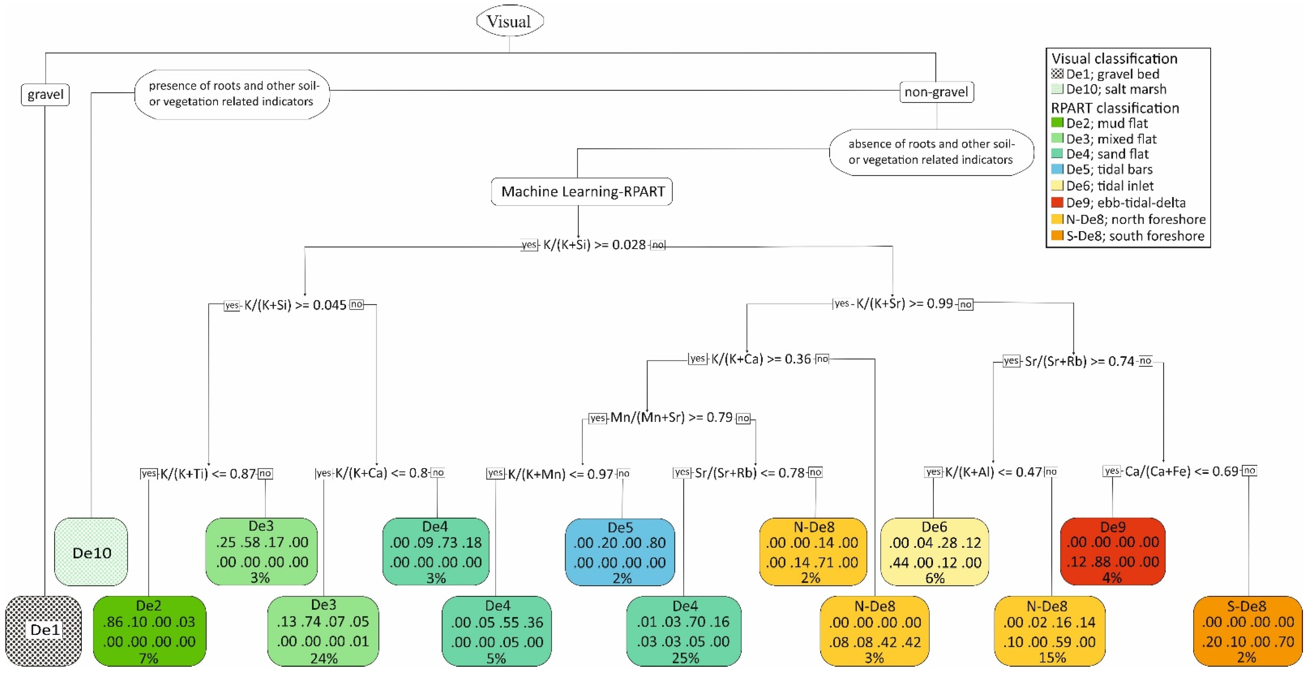
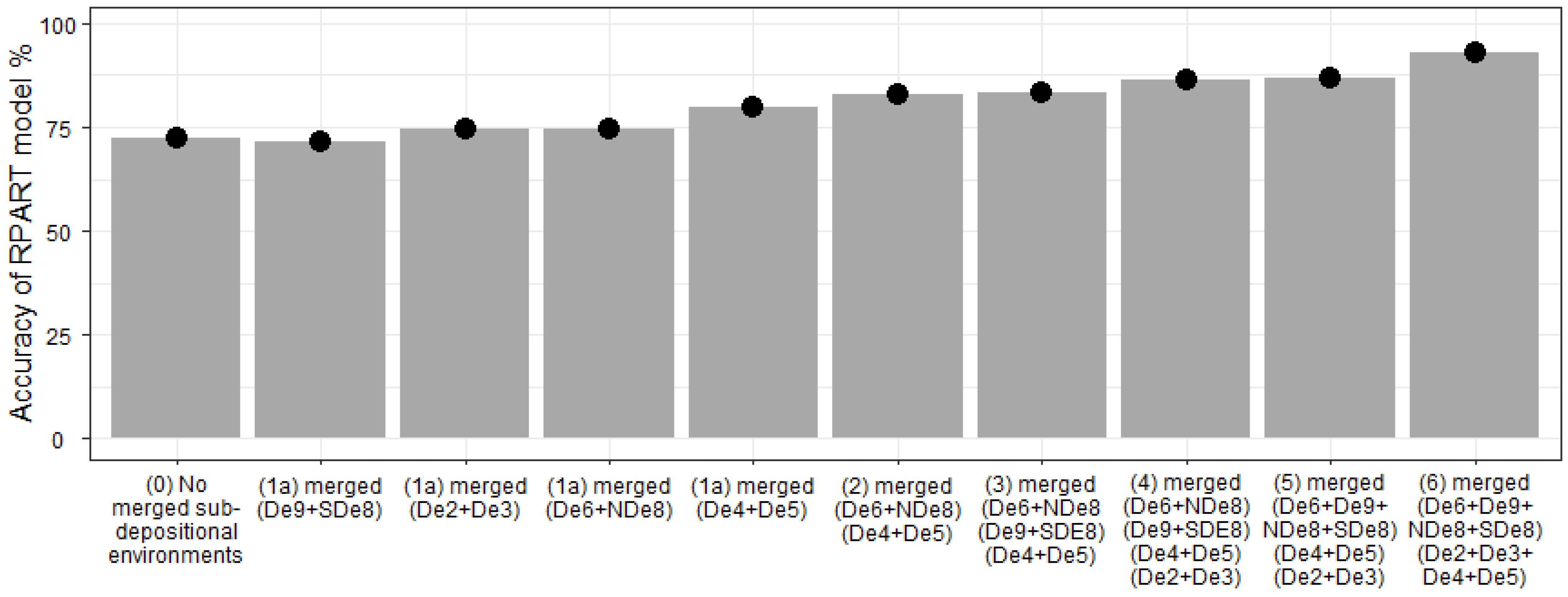
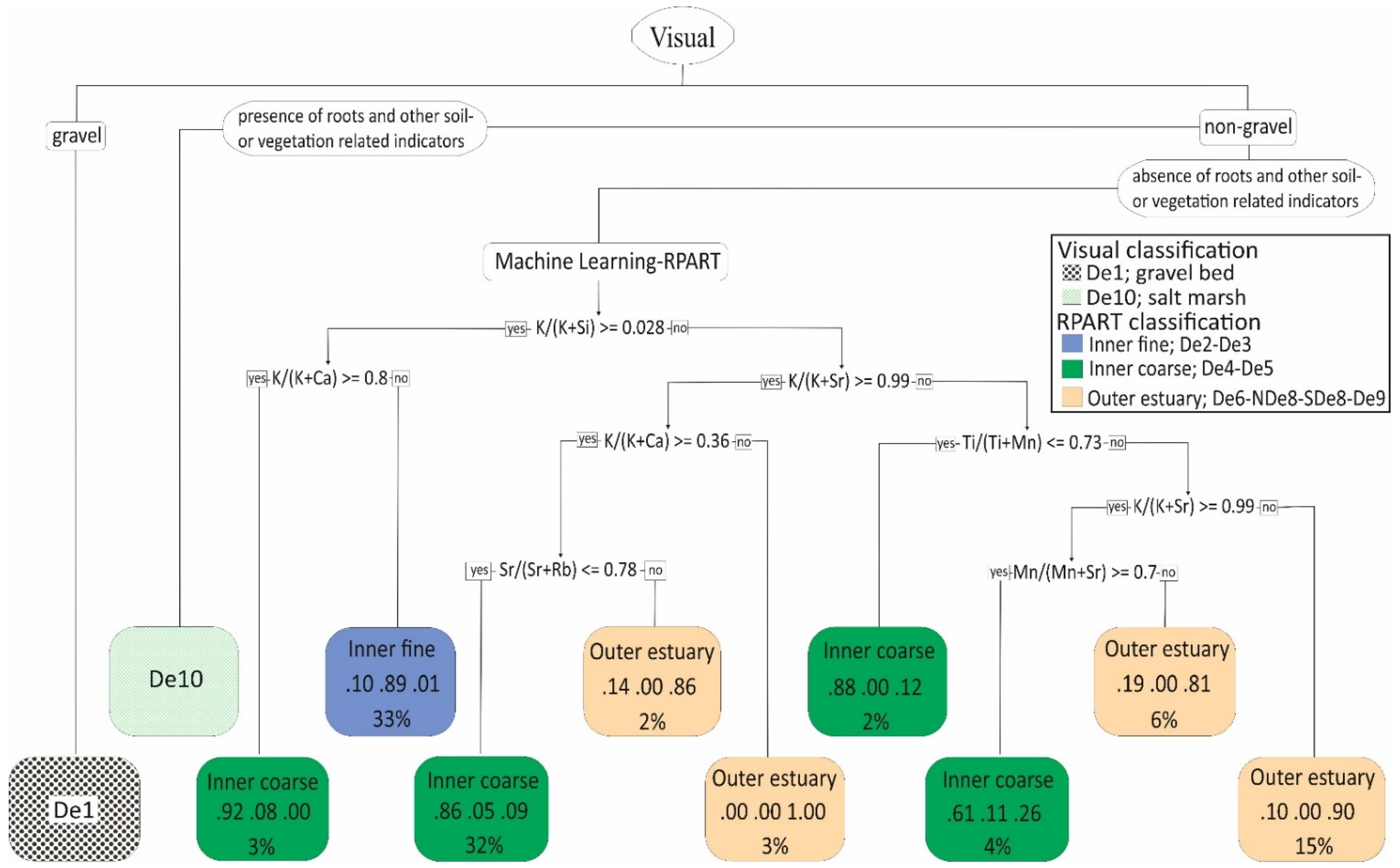
5.5. Development and Application of A Classification Diagram Using a Supervised Machine Learning Approach (RPART)

The results of the statistical ANOVA and HSD tests (Table 4) can also be visualised using the boxplots in Figure 7 [95,96]. We have here illustrated boxplots of the key indices K/(K + Si), K/(K + Ca), Mn/(Mn + Sr), K/(K + Al), K/(K + Mn), K/(K + Ti), K/(K + Sr), Sr/(Sr + Rb), and Ca/(Ca + Fe), all of which will be used to differentiate the estuarine sub-depositional environment (Figure 7).
The combination of initial visual discrimination of gravel beds and root-bearing salt marsh, followed by the use of numerous element indices via a supervised machine learning approach, in the form of recursive partitioning (RPART), has led to a new quantitative classification approach to discriminate sub-depositional environments in an estuarine setting.
The RPART package [73], available in R statistical software [70], was employed to classify the geochemical signatures of sediments into sub-depositional environments. We employed Recursive Partitioning and Regression Tree (RPART) software in R to develop a classification tree by using elemental indices to find best splits for the dataset into different sub-depositional environments in the Ravenglass Estuary. A similar approach was employed by Simon et al. [52] to subdivide sediment textural data from the Ravenglass Estuary. It was hoped that the geochemical data might lead to an improved classification compared to the textural data; note that the risk of closed datasets [97], has here been circumvented by using element indices.
Classification trees, derived by machine learning, create quantitative decision node split-points for a given index. The software establishes the dominant discriminators; these sit highest up the tree. The RPART-supervised machine learning approach (Figure 9) selected decision nodes of the following elemental indices to achieve a supervised classification: K/(K + Si), K/(K + Al), K/(K + Ca), K/(K + Ti), K/(K + Mn), K/(K + Sr), Sr/(Sr + Rb), Ca/(Ca + Fe), and Mn/(Mn + Sr). Initially, we trained the model to identify all eight sub-depositional environments: De2, De3, De4, De5, De6, NDe8, SDe8 and De9. At the end of each branch, there is either another decision node or a terminal leaf node. For each terminal leaf node, the software states the sub-depositional environment that has the highest probability (i.e., the name or the “answer”), but it also lists the fractional probability of each sub-depositional environment in the order in which they are listed in the key. The percentage of all samples in that terminal leaf node is also stated. The classification is most successful when the highest fractional values in each leaf node are close to 1.00. Values are less than 1.00 when there are overlaps in the geochemical attributes of two or more sub-depositional environments.
The decision nodes each relate to a specific question imposed on the data by the software, in terms of whether values are greater or less than a given value for a specific index (Figure 9). We have transposed the critical values for the software-selected optimal indices onto the boxplots in Figure 7. For example, towards the left-hand side of the classification diagram, K/(K + Ti) has a critical value of 0.87, whereby if samples are less than this value, there is an 86% probability that the samples are from mud flat sub-depositional environments. We have superimposed the value of 0.87 as a dashed line on Figure 7F, which illustrates the previous point about discriminating De2 and De3 sediments.
The code in R can be used to evaluate the accuracy of the RPART classification. In the case of the eight sub-depositional environments, the accuracy is 72.3% (Figure 10). We have engineered the dataset, to try to achieve higher-accuracy models, by selectively merging neighbouring sub-depositional environments. The most accurate classification model resulted from merging all inner estuary sediments (De2, De3, De4, and De5) and all outer estuary sediments (De6, De9, NDe8, and NDe8), leading to an accuracy of 92.9% (Figure 10). One of the single biggest improvements is in the merging of sand flat and tidal bar sediment (De4 and De5) sediments, as this led to a 7.5% increase in the model accuracy (Figure 10).
We have here displayed one of the simpler classification trees, based on partly merged sub-depositional environments (Figure 11). This model was developed with all outer estuary sediments grouped (De6, De9, NDe8, and NDe8) but leaving inner estuary sediments grouped into coarser (De4 and De5) and finer (De2 and De3) sediments. This classification approach led to a model accuracy of 87.0% (Figure 10 and Figure 11).
The method proposed above, calibrated with geochemical data from the Ravenglass Estuary surface sediments from known sub-depositional environments, has been applied to the geochemical data from the Holocene core (Figure 8).

5.6. Application of Proposed Model for Discrimination of Estuarine Sub-Environments

We have applied the fully resolved RPART model (no merging of sub-depositional environments) (Figure 9) to the geochemical data from the Holocene core (Figure 8). The output from the application of the model has allowed us to define palaeo-sub-depositional environments, instead of using an indirect method of describing sedimentary facies, grouping these into facies associations and then interpreting palaeo-sub-depositional environments [58]. We first applied visual identification to establish the presence of gravel beds and salt marsh in the core. Using our new approach, we were able to identify mud flat, mixed flat, sand flat, tidal bar, tidal inlet, northern foreshore, and ebb-tidal delta sub-depositional environments throughout the core interval (Figure 12).
In detail, the massive, texturally-bland, section between a depth of 300 and 400 cm was hard to interpret in terms of descriptive facies-based analysis. On the basis of core description, the sand between depths of 300 and 400 cm may have been due to inner or outer estuary deposition, given the lack of diagnostic sediment structures, trace fossils, or other features. The application of the automated classification approach has here revealed that this section was due to inner estuary deposition.
The sediment accumulation in this core started with a late glacial event and the accumulation of glacial diamicton [58]. The first sediments preserved on top of the till were apparently from a marine outer estuary environment (De9, Figure 12). This was succeeded by 100 cm of sand bar deposits (De4) and then approximately 200 cm of interbedded sand flat and mixed flat deposits (De3, Figure 12). The final 100 cm of deposition represents salt marsh deposits. This overall sequence could represent a time of (a) falling sea level, or (b) a greater rate of delivery of sediment to the estuary compared to net flux to the ocean. Salt marsh commonly represents the final stages of the levelling of marine coastal plains and the presence of marsh above the implies a phase of abandonment due to river migration [58]. Overall, the Holocene core shows an upward-fining profile at the multi-metre scale and represents a highstand-into-regression sequence. The newly revised interpretation, based on the geochemical classification of sub-depositional environments, shows that the core, drilled into a present-day tidal bar sub-depositional environment, was not always the site of a tidal bar throughout the Holocene.
The interpretation of the occurrence of a few discrete samples of northern foreshore and tidal inlet sediments is probably anomalous and a consequence of the fact that the RPART models are not 100% accurate, as shown by the leaf nodes in the classification diagram not having values of 1.0 in the dominant sub-depositional environment (Figure 9 and Figure 11). It is probably appropriate to be led by the overall stacking pattern of the sediments rather than be driven by potentially anomalous 5 cm beds that seem to be out of sequence. Note that this interpretation is based on the concept that all environments in the core exist in the estuary at the present time; this assumption is reasonable but is difficult to unequivocally prove.
A question remains about the significance of the interpretation of the basal ebb-tidal delta sediments in Figure 12. This question arises as there are no intermediate sediments from foreshore, tidal inlet or tidal bar sub-depositional environments between the ebb-tidal delta and sand flat successions, thus seeming to break Walther’s law. It seems unlikely that sand flat deposits would sit directly on top of ebb-tidal delta deposits as they are not adjacent sub-depositional environments. There is no sign of erosion of intermediate sediment between tidal delta and sand flat deposits (Figure 8). The significance of the ebb-tidal delta sub-depositional environment in the core in Figure 12 is unclear, but it may be due to mis-classification due to overlapping characteristics of the ebb-tidal delta and sand flat sediments. Despite this question, the development of a ML-approach, using a surface sediment calibration dataset, has proved to be a valuable tool to better understand palaeo-environments in 10,000 years of post-Holocene deposition recorded in a core.
This novel geochemical classification of sub-depositional environments has a good level of accuracy at discriminating outer estuary sediments, fine-grained inner estuary sediments and coarse-grained inner estuary sediments. It can also differentiate eight sub-depositional environments but with a lower degree of accuracy than the less refined classification scheme. The Ravenglass classification models (Figure 9 and Figure 11) may be applicable to other estuaries but differences in provenance and in-basin geochemical processes may result in different cut-offs at decision nodes: such an approach remains to be tested. It is also possible that the geochemical indices, that proved to be useful at differentiating modern and Holocene sub-depositional environments, could also be effective for estuarine cores from deeply buried and ancient sandstones. As a final point, the approach laid out here could also be applied to other modern and ancient depositional environments that also have subtleties that are not easy to differentiate using classical core description and facies analysis approaches.

6. Conclusions

  • This work represents a detailed study of sediment, analysed for composition using pXRF analyses, from the Ravenglass Estuary, NW England, United Kingdom.
  • Sub-depositional environments, mapped and defined across the estuary, include gravel beds, salt marsh, mud flats, mixed flats, sand flats, tidal bars, tidal inlet, foreshore, and ebb-tidal delta. The foreshore of the Ravenglass Estuary was subdivided into discrete northern and southern portions as they have distinct textural and elemental attributes.
  • Elements concentrations vary throughout the estuary, especially in terms of localised differences of Al, K, Ca, Fe, Mn, Zr, Rb, some of which will be the result of localised dilution due to preferential accumulation of detrital quartz.
  • Major, minor and trace element indices, varying between 0 and 1, were employed for the discrimination of sub-depositional environments, instead of raw concentration data, to circumvent the problem of variable dilution by quartz and closed datasets.
  • Element indices are heterogeneously distributed throughout the estuary, showing that element concentration patterns are not simply due to variable dilution by quartz.
  • There are strong relationships between specific sub-depositional environments and element indices within the estuary.
  • Provenance, sediment mineralogy and grain size, controlled by estuarine hydrodynamics, are the dominant controls on the distribution of elements (and their indices) in the Ravenglass Estuary.
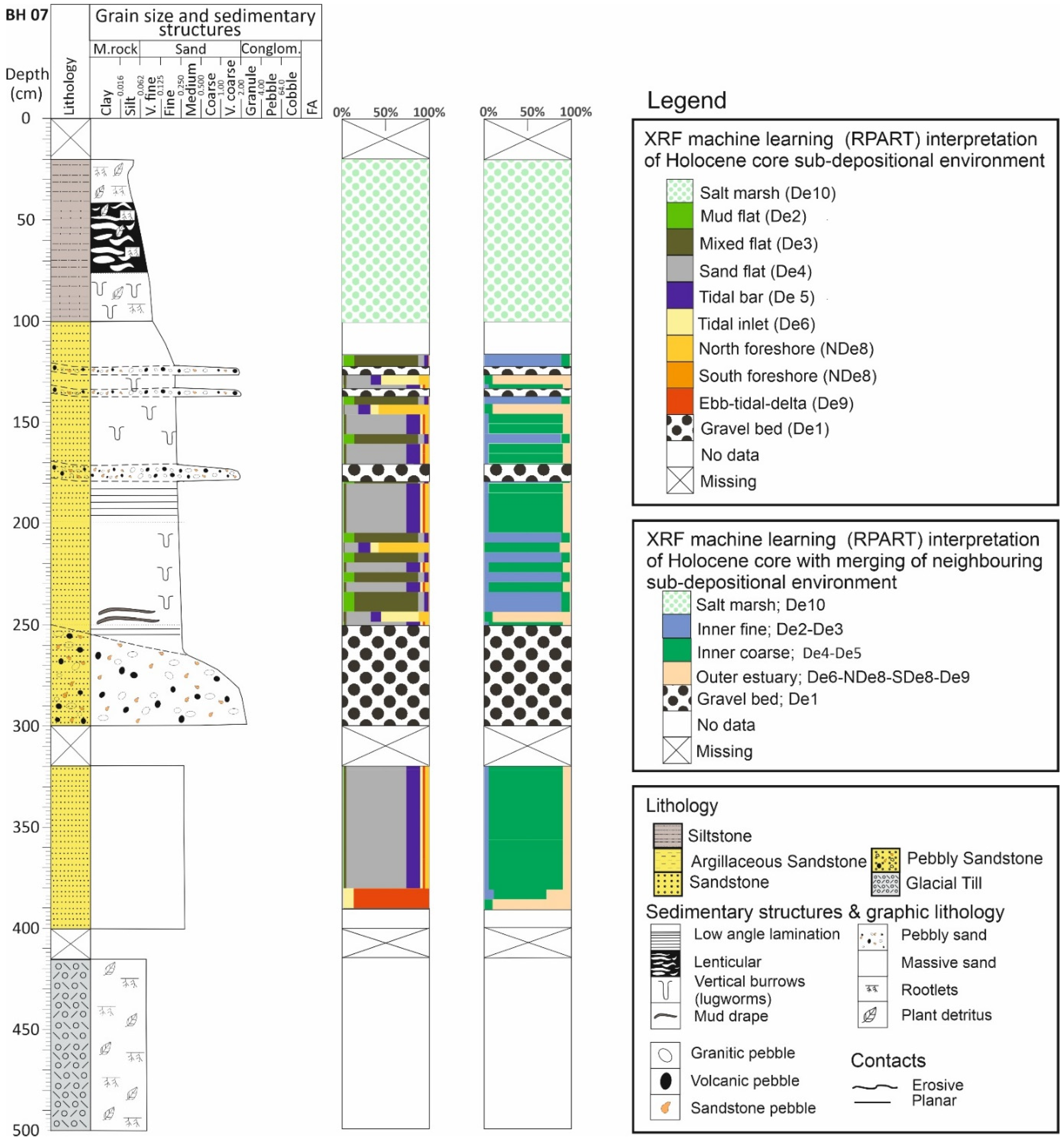
  • A supervised machine learning method was developed, using the RPART routine in R Statistical Software, for the automatic discrimination of palaeo sub-depositional environments, with the model calibrated using surface sediment element indices. The model was successfully applied to a core drilled through the Holocene succession at Ravenglass to predict palaeo sub-depositional environments over the last 10,000 years.
  • This work has proved that there are strong and predictable relationships between estuarine sub-depositional environments and sediment geochemistry.

Author Contributions

Conceptualisation, R.H.W.; Data curation, D.D.M.; Formal analysis, D.D.M., N.S., J.E.P.U., J.G. and L.J.W.; Funding acquisition, R.H.W.; Investigation, D.D.M. and N.S.; Resources, R.H.W.; Supervision, R.H.W., I.T.E.V. and R.A.D.; Writing—original draft, D.D.M.; Writing—review & editing, R.H.W., N.S., J.E.P.U., I.T.E.V., R.A.D., J.G. and L.J.W. All authors have read and agreed to the published version of the manuscript.

Funding

This research project was funded by the Nigerian Petroleum Technology Development Fund (PTDF).

Institutional Review Board Statement

Not applicable.

Informed Consent Statement

Not applicable.

Data Availability Statement

Not applicable.

Conflicts of Interest

The authors declare no conflict of interest. The sponsors had no influence on the research topic, data collection, analyses and the conclusions of this study.

References

  1. Rui, Z.; Lu, J.; Zhang, Z.; Guo, R.; Ling, K.; Zhang, R.; Patil, S. A quantitative oil and gas reservoir evaluation system for development. J. Nat. Gas Sci. Eng. 2017, 42, 31–39. [Google Scholar] [CrossRef]
  2. Worden, R.H.; Armitage, P.J.; Butcher, A.R.; Churchill, J.M.; Csoma, A.E.; Hollis, C.; Lander, R.H.; Omma, J.E. Petroleum reservoir quality prediction: Overview and contrasting approaches from sandstone and carbonate communities. Geol. Soc. Lond. Spec. Publ. 2018, 435, 1–31. [Google Scholar] [CrossRef]
  3. Zahid, M.A.; Chunmei, D.; Lin, C.; Gluyas, J.; Jones, S.; Zhang, X.; Munawar, M.J.; Ma, C. Sequence stratigraphy, sedimentary facies and reservoir quality of Es4s, southern slope of Dongying Depression, Bohai Bay Basin, East China. Mar. Pet. Geol. 2016, 77, 448–470. [Google Scholar] [CrossRef]
  4. Haile, B.G.; Klausen, T.G.; Czarniecka, U.; Xi, K.; Jahren, J.; Hellevang, H. How are diagenesis and reservoir quality linked to depositional facies? A deltaic succession, Edgeoya, Svalbard. Mar. Pet. Geol. 2018, 92, 519–546. [Google Scholar] [CrossRef]
  5. Chan, M.A. Correlations of diagenesis with sedimentary facies in Eocene sandstones, western Oregon. J. Sediment. Petrol. 1985, 55, 322–333. [Google Scholar]
  6. Anderton, R. Clastic facies models and facies analysis. Geol. Soc. Lond. Spec. Publ. 1985, 18, 31–47. [Google Scholar] [CrossRef]
  7. Dalrymple, R.W.; Choi, K. Morphologic and facies trends through the fluvial–marine transition in tide-dominated depositional systems: A schematic framework for environmental and sequence-stratigraphic interpretation. Earth-Sci. Rev. 2007, 81, 135–174. [Google Scholar] [CrossRef]
  8. Martinius, A.W.; Ringrose, P.S.; Brostrom, C.; Elfenbein, C.; Naess, A.; Ringas, J.E. Reservoir challenges of heterolithic tidal sandstone reservoirs in the Halten Terrace, mid-Norway. Pet. Geosci. 2005, 11, 3–16. [Google Scholar] [CrossRef]
  9. Primmer, T.J.; Cade, C.A.; Evans, J.; Gluyas, J.; Hopkins, M.S.; Oxtoby, N.; Smalley, P.C.; Warren, E.A.; Worden, R.H. Global patterns in sandstone diagenesis: Their application to reservoir quality prediction for petroleum exploration. In Reservoir Quality Prediction in Sandstones and Carbonates. AAPG Memoir; Kupecz, J.A., Gluyas, J., Bloch, S., Eds.; American Association of Petroleum Geologists: Tulsa, OK, USA, 1997; Volume 69, pp. 61–78. [Google Scholar]
  10. Berner, E.K.; Berner, R.A. Global Environment: Water, Air, and Geochemical Cycles; Princeton University Press: Princeton, NJ, USA, 2012. [Google Scholar]
  11. Boyle, E.A.; Edmond, J.M.; Sholkovitz, E.R. Mechanism of iron removal in estuaries. Geochim. Cosmochim. Acta 1977, 41, 1313–1324. [Google Scholar] [CrossRef]
  12. Coynel, A.; Schäfer, J.; Blanc, G.; Bossy, C. Scenario of particulate trace metal and metalloid transport during a major flood event inferred from transient geochemical signals. Appl. Geochem. 2007, 22, 821–836. [Google Scholar] [CrossRef]
  13. Lanceleur, L.; Schäfer, J.; Blanc, G.; Coynel, A.; Bossy, C.; Baudrimont, M.; Glé, C.; Larrose, A.; Renault, S.; Strady, E. Silver behaviour along the salinity gradient of the Gironde Estuary. Environ. Sci. Pollut. Res. 2013, 20, 1352–1366. [Google Scholar] [CrossRef]
  14. Elbaz-Poulichet, F.; Martin, J.; Huang, W.; Zhu, J. Dissolved Cd behaviour in some selected French and Chinese estuaries. Consequences on Cd supply to the ocean. Mar. Chem. 1987, 22, 125–136. [Google Scholar] [CrossRef]
  15. Dabrin, A.; Schäfer, J.; Blanc, G.; Strady, E.; Masson, M.; Bossy, C.; Castelle, S.; Girardot, N.; Coynel, A. Improving estuarine net flux estimates for dissolved cadmium export at the annual timescale: Application to the Gironde Estuary. Estuar. Coast. Shelf Sci. 2009, 84, 429–439. [Google Scholar] [CrossRef]
  16. Audry, S.; Blanc, G.; Schäfer, J.; Chaillou, G.; Robert, S. Early diagenesis of trace metals (Cd, Cu, Co, Ni, U, Mo, and V) in the freshwater reaches of a macrotidal estuary. Geochim. Cosmochim. Acta 2006, 70, 2264–2282. [Google Scholar] [CrossRef]
  17. Dyer, K.R. Estuaries: A Physical Introduction; Wiley: New York, NY, USA, 1997; Volume 1. [Google Scholar]
  18. Zwingmann, H.; Clauer, N.; Gaupp, R. Structure-related geochemical (REE) and isotopic (K-Ar, Rb-Sr, δ18O) characteristics of clay minerals from Rotliegend sandstone reservoirs (Permian, northern Germany). Geochim. Cosmochim. Acta 1999, 63, 2805–2823. [Google Scholar] [CrossRef]
  19. Smith, D.B.; Woodruff, L.G.; O’Leary, R.M.; Cannon, W.F.; Garrett, R.G.; Kilburn, J.E.; Goldhaber, M.B. Pilot studies for the North American Soil Geochemical Landscapes Project–site selection, sampling protocols, analytical methods, and quality control protocols. Appl. Geochem. 2009, 24, 1357–1368. [Google Scholar] [CrossRef]
  20. Meinhold, G.; Kostopoulos, D.; Reischmann, T. Geochemical constraints on the provenance and depositional setting of sedimentary rocks from the islands of Chios, Inousses and Psara, Aegean Sea, Greece: Implications for the evolution of Palaeotethys. J. Geol. Soc. 2007, 164, 1145–1163. [Google Scholar] [CrossRef] [Green Version]
  21. Yardley, B.W.D. An Introduction to Metamorphic Petrology; Longman: Harlow, UK, 1989. [Google Scholar]
  22. Fralick, P.; Kronberg, B. Geochemical discrimination of clastic sedimentary rock sources. Sediment. Geol. 1997, 113, 111–124. [Google Scholar] [CrossRef]
  23. Flood, R.P.; Bloemsma, M.R.; Weltje, G.J.; Barr, I.D.; O’Rourke, S.M.; Turner, J.N.; Orford, J.D. Compositional data analysis of Holocene sediments from the West Bengal Sundarbans, India: Geochemical proxies for grain-size variability in a delta environment. Appl. Geochem. 2016, 75, 222–235. [Google Scholar] [CrossRef]
  24. Dinelli, E.; Tateo, F.; Summa, V. Geochemical and mineralogical proxies for grain size in mudstones and siltstones from the Pleistocene and Holocene of the Po River alluvial plain, Italy. In Proceedings of the Symposium on Sedimentary Provenance and Petrogenesis held at the 32nd International Geological Congress, Florence, Italy, 20–28 August 2004; pp. 25–36. [Google Scholar]
  25. Folk, R.L. A review of grain-size parameters. Sedimentology 1966, 6, 73–93. [Google Scholar] [CrossRef]
  26. Folk, R.L. Petrology of sedimentary rocks: Hemphill’s. Austin Tex. 1968, 170, 85. [Google Scholar]
  27. Rowe, H.; Hughes, N.; Robinson, K. The quantification and application of handheld energy-dispersive x-ray fluorescence (ED-XRF) in mudrock chemostratigraphy and geochemistry. Chem. Geol. 2012, 324, 122–131. [Google Scholar] [CrossRef]
  28. Morris, P.A. Field-Portable X-ray Fluorescence Analysis and Its Application in GSWA; Geological Survey of Western Australia: Perth, Australia, 2009. [Google Scholar]
  29. Gazley, M.F.; Vry, J.K.; du Plessis, E.; Handler, M.R. Application of portable X-ray fluorescence analyses to metabasalt stratigraphy, Plutonic Gold Mine, Western Australia. J. Geochem. Explor. 2011, 110, 74–80. [Google Scholar] [CrossRef]
  30. Weindorf, D.C.; Zhu, Y.; Chakraborty, S.; Bakr, N.; Huang, B. Use of portable X-ray fluorescence spectrometry for environmental quality assessment of peri-urban agriculture. Environ. Monit. Assess. 2012, 184, 217–227. [Google Scholar] [CrossRef]
  31. McLaren, T.I.; Guppy, C.N.; Tighe, M.K.; Forster, N.; Grave, P.; Lisle, L.M.; Bennett, J.W. Rapid, nondestructive total elemental analysis of vertisol soils using portable X-ray fluorescence. Soil Sci. Soc. Am. J. 2012, 76, 1436–1445. [Google Scholar] [CrossRef] [Green Version]
  32. Kenna, T.C.; Nitsche, F.O.; Herron, M.M.; Mailloux, B.J.; Peteet, D.; Sritrairat, S.; Sands, E.; Baumgarten, J. Evaluation and calibration of a Field Portable X-Ray Fluorescence spectrometer for quantitative analysis of siliciclastic soils and sediments. J. Anal. At. Spectrom. 2011, 26, 395–405. [Google Scholar] [CrossRef]
  33. Plourde, A.; Knight, R.; Kjarsgaard, B.; Sharpe, D.; Lesemann, J. Portable XRF spectrometry of surficial sediments, NTS 75-I, 75-J, 75-O, 75-P (Mary Frances Lake–Whitefish Lake–Thelon River area), Northwest Territories. Geol. Surv. Can. Open File 2013, 7408, 25. [Google Scholar]
  34. Turner, J.N.; Jones, A.F.; Brewer, P.A.; Macklin, M.G.; Rassner, S.M. Micro-XRF applications in fluvial sedimentary environments of Britain and Ireland: Progress and prospects. In Micro-XRF Studies of Sediment Cores; Springer: Berlin/Heidelberg, Germany, 2015; pp. 227–265. [Google Scholar]
  35. Potts, P.J. Introduction, analytical instrumentation and application overview. In Portable X-ray Fluorescence Spectrometry: Capabilities for In Situ Analysis; The Royal Society of Chemistry: London, UK, 2008; pp. 1–12. [Google Scholar]
  36. Rollinson, H.R. Using Geochemical Data: Evaluation, Presentation, Interpretation; Routledge: Oxfordshire, UK, 2014. [Google Scholar]
  37. Benn, C. Lithological discrimination in deeply weathered terrains using multielemental geochemistry–an example from the Yanfolila gold project, Mali. Explore 2012, 156, 1–8. [Google Scholar]
  38. Marsala, A.; Loermans, T.; Shen, S.; Scheibe, C.; Zereik, R. Portable energy-dispersive X-ray fluorescence integrates mineralogy and chemostratigraphy into real-time formation evaluation. Petrophysics 2012, 53, 102–109. [Google Scholar]
  39. Le Vaillant, M.; Barnes, S.J.; Fiorentini, M.L.; Santaguida, F.; Törmänen, T. Effects of hydrous alteration on the distribution of base metals and platinum group elements within the Kevitsa magmatic nickel sulphide deposit. Ore Geol. Rev. 2016, 72, 128–148. [Google Scholar] [CrossRef]
  40. Young, K.E.; Evans, C.A.; Hodges, K.V.; Bleacher, J.E.; Graff, T.G. A review of the handheld X-ray fluorescence spectrometer as a tool for field geologic investigations on Earth and in planetary surface exploration. Appl. Geochem. 2016, 72, 77–87. [Google Scholar] [CrossRef] [Green Version]
  41. Emmerson, R.; O’Reilly-Wiese, S.; Macleod, C.; Lester, J. A multivariate assessment of metal distribution in inter-tidal sediments of the Blackwater Estuary, UK. Mar. Pollut. Bull. 1997, 34, 960–968. [Google Scholar] [CrossRef]
  42. Martins, R.; Azevedo, M.; Mamede, R.; Sousa, B.; Freitas, R.; Rocha, F.; Quintino, V.; Rodrigues, A. Sedimentary and geochemical characterization and provenance of the Portuguese continental shelf soft-bottom sediments. J. Mar. Syst. 2012, 91, 41–52. [Google Scholar] [CrossRef]
  43. Ross, P.-S.; Bourke, A.; Fresia, B. Improving lithological discrimination in exploration drill-cores using portable X-ray fluorescence measurements: (1) testing three Olympus Innov-X analysers on unprepared cores. Geochem. Explor. Environ. Anal. 2014, 14, 171–185. [Google Scholar] [CrossRef]
  44. Yuan, Z.; Cheng, Q.; Xia, Q.; Yao, L.; Chen, Z.; Zuo, R.; Xu, D. Spatial patterns of geochemical elements measured on rock surfaces by portable X-ray fluorescence: Application to hand specimens and rock outcrops. Geochem. Explor. Environ. Anal. 2014, 14, 265–276. [Google Scholar] [CrossRef]
  45. Wooldridge, L.J.; Worden, R.H.; Griffiths, J.; Utley, J.E.P. Clay-coated sand grains in petroleum reservoirs: Understanding their distribution via a modern analogue. J. Sediment. Res. 2017, 87, 338–352. [Google Scholar] [CrossRef]
  46. Wooldridge, L.J.; Worden, R.H.; Griffiths, J.; Thompson, A.; Chung, P. Biofilm origin of clay-coated sand grains. Geology 2017, 45, 875–878. [Google Scholar] [CrossRef] [Green Version]
  47. Griffiths, J.; Worden, R.H.; Wooldridge, L.J.; Utley, J.E.; Duller, R.A.; Edge, R.L. Estuarine clay mineral distribution: Modern analogue for ancient sandstone reservoir quality prediction. Sedimentology 2019, 66, 2011–2047. [Google Scholar] [CrossRef]
  48. Griffiths, J.; Worden, R.H.; Wooldridge, L.J.; Utley, J.E.; Duller, R.A. Compositional variation in modern estuarine sands: Predicting major controls on sandstone reservoir quality. AAPG Bull. 2019, 103, 797–833. [Google Scholar] [CrossRef]
  49. Griffiths, J.; Worden, R.H.; Wooldridge, L.J.; Utley, J.E.; Duller, R.A. Detrital clay coats, clay minerals, and pyrite: A modern shallow-core analogue for ancient and deeply buried estuarine sandstones. J. Sediment. Res. 2018, 88, 1205–1237. [Google Scholar] [CrossRef] [Green Version]
  50. Daneshvar, E.; Worden, R.H. Feldspar alteration and Fe minerals: Origin, distribution and implications for sandstone reservoir quality in estuarine sediments. Geol. Soc. Lond. Spec. Publ. 2017, 435, 123–139. [Google Scholar] [CrossRef]
  51. Daneshvar, E. Dissolved iron behavior in the Ravenglass Estuary waters, an implication on the early diagenesis. Univers. J. Geosci. 2015, 3, 1–12. [Google Scholar] [CrossRef] [Green Version]
  52. Simon, N.; Worden, R.H.; Muhammed, D.D.; Utley, J.E.P.; Verhagen, I.T.E.; Griffiths, J.; Wooldridge, L.J. Sediment textural characteristics of the Ravenglass Estuary; Development of a method to predict palaeo sub-depositional environments from estuary core samples. Sediment. Geol. 2021, 418, 105906. [Google Scholar] [CrossRef]
  53. Lloyd, J.M.; Zong, Y.; Fish, P.; Innes, J.B. Holocene and Late-glacial relative sea-level change in north-west England: Implications for glacial isostatic adjustment models. J. Quat. Sci. 2013, 28, 59–70. [Google Scholar] [CrossRef]
  54. Bousher, A. Ravenglass Estuary: Basic Characteristics and Evaluation of Restoration Options; Westlakes Scientific Consulting: Whitehaven, UK, 1999. [Google Scholar]
  55. Kelly, M.; Emptage, M.; Mudge, S.; Bradshaw, K.; Hamilton-Taylor, J. The relationship between sediment and plutonium budgets in a small macrotidal estuary—Esk Estuary, Cumbria, UK. J. Environ. Radioact. 1991, 13, 55–74. [Google Scholar] [CrossRef]
  56. Carr, A.P.; Blackley, M.W.L. Implications of sedimentological and hydrological processes on the distribution of radionuclides: The example of a salt marsh near Ravenglass, Cumbria. Estuar. Coast. Shelf Sci. 1986, 22, 529–543. [Google Scholar] [CrossRef]
  57. Merritt, J.; Auton, C. An outline of the lithostratigraphy and depositional history of Quaternary deposits in the Sellafield district, west Cumbria. Proc. Yorks Geol. Soc. 2000, 53, 129–154. [Google Scholar] [CrossRef]
  58. McGhee, C.A.; Muhammed, D.D.; Simon, N.; Acikalin, S.; Utley, J.E.P.; Griffiths, J.; Wooldridge, L.M.; Verhagen, I.T.E.; van der Land, C.; Worden, R.H. Stratigraphy and sedimentary evolution of a modern macro-tidal incised valley—An analogue for reservoir facies and architecture. Sedimentology 2021. [Google Scholar] [CrossRef]
  59. Brockamp, O.; Zuther, M. Changes in clay mineral content of tidal flat sediments resulting from dike construction along the Lower Saxony coast of the North Sea, Germany. Sedimentology 2004, 51, 591–600. [Google Scholar] [CrossRef]
  60. Gutiérrez-Ginés, M.J.; Pastor, J.; Hernández, A.J. Assessment of field portable X-ray fluorescence spectrometry for the in situ determination of heavy metals in soils and plants. Environ. Sci. Processes Impacts 2013, 15, 1545–1552. [Google Scholar] [CrossRef] [PubMed] [Green Version]
  61. Chou, J.; Clement, G.; Bursavich, B.; Elbers, D.; Cao, B.; Zhou, W. Rapid detection of toxic metals in non-crushed oyster shells by portable X-ray fluorescence spectrometry. Environ. Pollut. 2010, 158, 2230–2234. [Google Scholar] [CrossRef] [PubMed]
  62. Carr, R.; Zhang, C.; Moles, N.; Harder, M. Identification and mapping of heavy metal pollution in soils of a sports ground in Galway City, Ireland, using a portable XRF analyser and GIS. Environ. Geochem. Health 2008, 30, 45–52. [Google Scholar] [CrossRef] [PubMed]
  63. Argyraki, A.; Ramsey, M.H.; Potts, P.J. Evaluation of portable X-ray fluorescence instrumentation for in situ measurements of lead on contaminated land. Analyst 1997, 122, 743–749. [Google Scholar] [CrossRef] [Green Version]
  64. Zarco-Perello, S.; Simões, N. Ordinary kriging vs. inverse distance weighting: Spatial interpolation of the sessile community of Madagascar reef, Gulf of Mexico. PeerJ 2017, 5, e4078. [Google Scholar] [CrossRef] [Green Version]
  65. Watson, D.F.; Philip, G.M. Comment on “a nonlinear empirical prescription for simultaneously interpolating and smoothing contours over an irregular grid” by F. Duggan. Comput. Methods Appl. Mech. Eng. 1985, 50, 195–198. [Google Scholar] [CrossRef]
  66. Grunsky, E.C.; Smee, B.W. The differentiation of soil types and mineralization from multi-element geochemistry using multivariate methods and digital topography. J. Geochem. Explor. 1999, 67, 287–299. [Google Scholar] [CrossRef]
  67. Cheng, Q.; Jing, L.; Panahi, A. Principal component analysis with optimum order sample correlation coefficient for image enhancement. Int. J. Remote Sens. 2006, 27, 3387–3401. [Google Scholar] [CrossRef]
  68. Michael, D.; Paul, D.; Andreas, S.; Mark, C. Principal component analysis of the geochemistry of soil developed on till in Northern Ireland. J. Maps 2013, 373. [Google Scholar]
  69. Klovan, J. The use of factor analysis in determining depositional environments from grain-size distributions. J. Sediment. Res. 1966, 36, 115–125. [Google Scholar] [CrossRef]
  70. R Core Team. R: A Language and Environment for Statistical Computing; R Foundation for Statistical Computing: Vienna, Austria, 2016. [Google Scholar]
  71. Scheffe, H. The Analysis of Variance; John Wiley & Sons: Hoboken, NJ, USA, 1999; Volume 72. [Google Scholar]
  72. Wickham, H. ggplot2: Elegant Graphics for Data Analysis; Springer: Berlin/Heidelberg, Germany, 2016. [Google Scholar]
  73. Therneau, T.; Atkinson, E. An Introduction to Recursive Partitioning Using Rpart Routines: The Comprehensive R Archive Network. 2019. Available online: https://cran.r-project.org/web/packages/rpart/vignettes/longintro.pdf (accessed on 10 November 2021).
  74. Reimann, C.; Filzmoser, P.; Garrett, R.; Dutter, R. Statistical Data Analysis Explained: Applied Environmental Statistics with R; John Wiley & Sons: Hoboken, NJ, USA, 2011. [Google Scholar]
  75. Herron, M.M. Geochemical classification of terrigenous sands and shales from core or log data. J. Sediment. Res. 1988, 58, 820–829. [Google Scholar] [CrossRef]
  76. Michalopoulos, P.; Aller, R.C. Rapid clay mineral transformation in Amazon Delta sediments—Reverse weathering and oceanic element cycles. Science 1995, 270, 614–617. [Google Scholar] [CrossRef]
  77. Aller, R.C.; Michalopoulos, P. Invited Lecture: Tropical, Mobile Mud Belts as Global Diagenetic Reactors; Balkema: Rotterdam, The Netherlands, 1999; pp. 289–292. [Google Scholar]
  78. Michalopoulos, P.; Aller, R.C.; Reeder, R.J. Conversion of diatoms to clays during early diagenesis in tropical, continental shelf muds. Geology 2000, 28, 1095–1098. [Google Scholar] [CrossRef]
  79. Nelson, B.W. Clay mineralogy of the bottom sediments, Rappahannock River, Virginia. In Clays and Clay Minerals, Proceedings of the Seventh National Conference on Clays and Clay Minerals, Washington, DC, USA, 20–23 Octorber 1958; Elsevier: Amsterdam, The Netherlands, 2013; pp. 135–148. [Google Scholar]
  80. Krauskopf, K.B.; Bird, D.K. Introduction to Geochemistry; McGraw-Hill: New York, NY, USA, 1967; Volume 721. [Google Scholar]
  81. Worden, R.H.; Griffiths, J.; Wooldridge, L.J.; Utley, J.E.P.; Lawan, A.Y.; Muhammed, D.D.; Simon, N.; Armitage, P.J. Chlorite in sandstones. Earth-Sci. Rev. 2020, 204, 103105. [Google Scholar] [CrossRef]
  82. Wooldridge, L.J.; Worden, R.H.; Griffiths, J.; Utley, J.E.P. Clay-coat diversity in marginal marine sediments. Sedimentology 2019, 66, 1118–1138. [Google Scholar] [CrossRef]
  83. Baker, P.A.; Gieskes, J.M.; Elderfield, H. Diagenesis of carbonates in deep-sea sediments; evidence from Sr/Ca ratios and interstitial dissolved Sr2+ data. J. Sediment. Res. 1982, 52, 71–82. [Google Scholar]
  84. Brookins, D.G. Strontium. In Eh-pH Diagrams for Geochemistry; Springer: Berlin/Heidelberg, Germany, 1988; pp. 166–167. [Google Scholar]
  85. Andrew-Oha, I.; Mosto-Onuoha, K.; Sunday-Dada, S. Contrasting styles of lead-zinc-barium mineralization in the Lower Benue Trough, Southeastern Nigeria. Earth Sci. Res. J. 2017, 21, 7–16. [Google Scholar]
  86. Rothwell, R.G.; Croudace, I.W. Twenty years of XRF core scanning marine sediments: What do geochemical proxies tell us? In Micro-XRF Studies of Sediment Cores: Applications of a Non-Destructive Tool Foe the Environmental Sciences; Developments in Paleoenvironmental Research; Croudace, I.W., Rothwell, R.G., Eds.; Springer: Dordrecht, The Netherlands, 2015; Volume 17, pp. 65–82. [Google Scholar]
  87. Hatch, J.; Leventhal, J. Relationship between inferred redox potential of the depositional environment and geochemistry of the Upper Pennsylvanian (Missourian) Stark Shale Member of the Dennis Limestone, Wabaunsee County, Kansas, USA. Chem. Geol. 1992, 99, 65–82. [Google Scholar] [CrossRef]
  88. Vaalgamaa, S.; Korhola, A. Geochemical signatures of two different coastal depositional environments within the same catchment. J. Paleolimnol. 2007, 38, 241–260. [Google Scholar] [CrossRef]
  89. Driskill, B.; Pickering, J.; Rowe, H. Interpretation of high resolution XRF data from the Bone Spring and Upper Wolfcamp, Delaware Basin, USA. In Proceedings of the Unconventional Resources Technology Conference, Houston, TX, USA, 23–25 July 2018; pp. 2861–2888. [Google Scholar]
  90. Calvert, S.; Pedersen, T. Chapter fourteen elemental proxies for palaeoclimatic and palaeoceanographic variability in marine sediments: Interpretation and application. Dev. Mar. Geol. 2007, 1, 567–644. [Google Scholar]
  91. Doerner, M.; Berner, U.; Erdmann, M.; Barth, T. Geochemical characterization of the depositional environment of Paleocene and Eocene sediments of the Tertiary Central Basin of Svalbard. Chem. Geol. 2020, 542, 119587. [Google Scholar] [CrossRef]
  92. Rübsam, W. The Early Toarcian Environmental Crisis: Mechanisms and Consequences of an Icehouse-Greenhouse Transition; Universitätsbibliothek Kiel: Kiel, Germany, 2019. [Google Scholar]
  93. Armstrong-Altrin, J.S.; Machain-Castillo, M.L.; Rosales-Hoz, L.; Carranza-Edwards, A.; Sanchez-Cabeza, J.-A.; Ruíz-Fernández, A.C. Provenance and depositional history of continental slope sediments in the Southwestern Gulf of Mexico unraveled by geochemical analysis. Cont. Shelf Res. 2015, 95, 15–26. [Google Scholar] [CrossRef]
  94. Mountney, N.P.; Thompson, D.B. Stratigraphic evolution and preservation of aeolian dune and damp/wet interdune strata: An example from the Triassic Helsby Sandstone Formation, Cheshire Basin, UK. Sedimentology 2002, 49, 805–833. [Google Scholar] [CrossRef]
  95. Hullman, J.; Resnick, P.; Adar, E. Hypothetical outcome plots outperform error bars and violin plots for inferences about reliability of variable ordering. PLoS ONE 2015, 10, e0142444. [Google Scholar]
  96. Hintze, J.L.; Nelson, R.D. Violin plots: A box plot-density trace synergism. Am. Stat. 1998, 52, 181–184. [Google Scholar]
  97. Aitchison, J. The Statistical Analysis of Compositional Data. J. R. Stat. Soc. Ser. B 1982, 44, 139–160. [Google Scholar] [CrossRef]
Figure 1. Location map of the Ravenglass Estuary, north-west England with an inset map showing the location of the estuary in the UK. The small yellow dots shows the distribution of surface-sediment sample site (<2 cm) used for XRF analysis and the larger purple dot shows the location of the geotechnical core.
Geosciences 12 00023 g001
Figure 2. Distribution of estuarine sub-depositional environments mapped across the Ravenglass Estuary. These sub-depositional environments are labelled; De1, gravel bed; De2, mud flat; De3, mixed flat; De4, sand flat; De5, tidal bars; De6, tidal inlet; De7, backshore; De8, foreshore (northern and southern sites); De9, ebb-tidal delta; and De10, salt marsh.
Geosciences 12 00023 g002
Figure 3. Frequency distribution curves of the mud, mixed and sand flat sub-depositional environments revealing how laser particle size analysis data were used to differentiate tidal flat sediments.
Geosciences 12 00023 g003
Figure 4. Spatial distribution of (A) grain size (mm), (B) aluminium (ppm, and for all other elements), (C) potassium, (D) calcium, (E) titanium, (F) iron, (G) manganese, (H) strontium, (I) rubidium, (J) zirconium, (K) barium, (L) and caesium within the Ravenglass Estuary. Note that mean grain size decreases towards the margins of the inner estuary and central basin and the grain size map (A) has had boundaries between sub-depositional environments from Figure 2 superimposed. The similarities in spatial distribution between Al and K with finer grain size, show potential control of mud on the distribution of these elements. Aluminium, K, Fe, Ti and Mn have their highest concentration across the inner estuary, upper reaches of Irt arm and tidal bars. Grain size as well as concentrations of Al, Ca and Rb are higher in the southern foreshore than the northern foreshore. The elements distribution pattern vary greatly with some apparent links to sub-depositional environment and geographic location.
Geosciences 12 00023 g004
Figure 5. Boxplots for texture and element concentrations as a function of the Ravenglass Estuary sub-depositional environment: (A) grain size (mm), (B) aluminium, (C) potassium, (D) calcium, (E) titanium, (F) iron, (G) manganese, (H) strontium, (I) rubidium, (J) zirconium, (K) barium, (L) caesium. Boxplots contain the median and upper and lower quartile ranges. Outliers are defined as > (or <) 1.5-times the interquartile range, above the upper and below the lower quartiles. Element concentrations vary greatly between different sub-depositional environments; for example, Ti and Fe concentrations are highest in the mud flat, and Rb and Sr concentrations are highest in the southern foreshore. Overall, the element concentrations in the sand-dominated sub-depositional environments show weak variability, potentially because of quartz dilution.
Geosciences 12 00023 g005
Figure 6. Spatial distribution of element indices (A) K/(K + Al), (B) K/(K + Si), (C) K/(K + Ca), (D) K/(K + Mn), (E) K/(K + Sr), (F) K/(K + Ti), (G) Ca/(Ca + Fe), (H) Mn/(Mn + Sr), (I) Sr/(Sr + Rb), (J) K/(K + Fe), (K) Fe/(Fe+Ti), and (L) Al/(Al + Fe) within the Ravenglass Estuary. Note that these element indices vary systematically for the Ravenglass Estuary sub-depositional environments. The combination of these elemental indices may be used to discriminate mud flat, mixed flat, sand flat, tidal bars, tidal inlet, north foreshore, south foreshore and ebb-tidal delta in the Ravenglass Estuary. Maps A to I represent the indices that RPART classification, in R Statistical Software, used to discriminate the various sub-depositional environments (see Section 5.5).
Geosciences 12 00023 g006
Figure 7. Box plots for element indices as a function of the Ravenglass Estuary depositional environment. (A) K/(K + Si), (B) K/(K + Ca), (C) Mn/(Mn + Sr), (D) K/(K + Al), (E) K/(K + Mn), (F) K/(K + Ti), (G) K/(K + Sr), (H) Sr/(Sr + Rb), (I) Ca/(Ca + Fe), (J) Ti/(Ti + Mn), (K) Fe/(Fe+Ti), and (L) Al/(Al + Fe). Boxplots contain the median and upper and lower quartile ranges. Outliers are defined as > (or <) 1.5-times the interquartile range, above the upper and below the lower quartiles. This figure should be examined in conjunction with Table 4 to reveal the most important differentiators between sub-depositional environments. The critical values for parts A to I have been taken from the machine learning-derived decision nodes (see Section 5.5).
Geosciences 12 00023 g007
Figure 8. Sedimentary log of the 5 m Holocene core drilled in a tidal bar in the Esk arm of the Ravenglass Estuary (Figure 1 and Figure 2) with the geochemical data, derived from XRF analysis, illustrated. These nine indices are represented as these are the ones that RPART classification, in R Statistical Software, used to discriminate the various sub-depositional environments (e.g., Section 5.5 and Figure 9). The critical values superimposed on the nine indices, were taken from machine learning-derived decision nodes in Figure 9.
Geosciences 12 00023 g008
Figure 9. Classification tree for the discrimination of estuarine sub-depositional environments, based on surface samples collected from the Ravenglass Estuary, developed through a combination of visual analysis (Figure 2) and pXRF analyses, using supervised classification and the recursive partitioning package, RPART [73], available in R studio software [70]. Each machine learning-derived decision node splits the data using one data (chemical index) type. In each terminal leaf node, the classification of depositional environment is listed first, followed by the fractional quantity of samples in the eight classified depositional environment; the higher the fractional quantities, the higher the classification certainty. Where these fractional values are less than 1.00, the uncertainty is because of some depositional environments having overlapping attributes, even when nine dimensions are considered. The value presented at the bottom of the node is the total percentage of the whole sample set that lies in each leaf node. This RPART-supervised machine learning approach differentiated De2, De3, De4, De5, De6, NDe8, SDe8 and De9 based on K/(K + Si), K/(K + Al), K/(K + Ca), K/(K + Ti), K/(K + Mn), K/(K + Sr), Sr/(Sr + Rb), Ca/(Ca + Fe), and Mn/(Mn + Sr) index data. This classification tree has a model accuracy of 72.3% (Figure 10).
Geosciences 12 00023 g009
Figure 10. Bar chart showing model accuracy for different approach of classification trees. High model accuracy was achieved by engineering the datasets, through selective merging of neighbouring sub-depositional environments.
Geosciences 12 00023 g010
Figure 11. Classification tree based on partly merged data, developed using the same approach as Figure 10. This classification tree has a model accuracy of 87.0% (Figure 10) and shows how high model accuracy can be achieved with subsequent grouping of neighbouring or near neighbouring, sub-depositional environments.
Geosciences 12 00023 g011
Figure 12. Schematic sedimentary log of the cored sediment beneath inner estuary vegetated tidal bar deposits (see Figure 1 for core location) with application of the classification tree in Figure 9 (wholly split sub-depositional environments) and Figure 11 (partly merged sub-depositional environments) to data presented in Figure 8. The split and merged geochemical classification models reveal a succession of sub-depositional environments that could not easily be predicted based only on classical core description methods.
Geosciences 12 00023 g012
Table 1. Factory reported detection limit for some key elements plus mean and standard deviations of one sample analysed 30 times to assess credibility of reported concentration data.
ElementReported Detection Limit (ppm)Mean of 30 Repeat Analyses from One Sample (ppm)Standard Deviation of 30 Repeat Analyses from One Sample (ppm)
Al200064,0991685
K25018,234145
Ca70261046
Ti6247792
Fe2511,83790
Mn3017219
Rb6701
Sr8732
Zr33523
Ba5048718
Cs12854
Table 2. Summary of geochemical elements identified by the handheld pXRF tool and number of samples for which the element is above the limit of detection.
Sub-EnvironmentSamplesAlSiPSClKCaScTiVCrMn
Foreshore6969691724696969369483567
Gravel bed2828281018282828428171926
Mixed flat949494154949494294516693
Mud flat5555551525555551655335254
Ebb-tidal delta2121219202121212216720
Sand flat120120120028120120120112010240113
Tidal bars535353012535353153431850
Tidal inlet2525255825252502520624
Salt marsh1717171717171717517141117
Sub-EnvironmentSamplesFeNiCuZnAsRbSrZrNbPdAg
Foreshore69690028156969692530
Gravel bed28270123132828281400
Mixed flat94940093209494948802
Mud flat55540055195555555500
Ebb-tidal delta212100142212121440
Sand flat1201190076121201201206900
Tidal bars5352103965353533102
Tidal inlet252511146252525721
Salt marsh17178117161717171323
Sub-EnvironmentSamplesCdSnSbTeCsBaHgPbBiThU
Foreshore691332206065693130148
Gravel bed281117102828280131143
Mixed flat9405115929394631465
Mud flat5502844854553118411
Ebb-tidal delta21172119212121019051
Sand flat1200642710611812022176
Tidal bars53035849535322131
Tidal inlet25417925252535081
Salt marsh171617171717171173157
Table 3. Summary of reported elements showing the minimum detected value for each in the Ravenglass Estuary.
ElementsAlSiPSClKCaScTi
Minimum value (ppm)124656,322119902662189736257
Samples above minimum value100%100%12%48%100%100%100%7%100%
ElementsVCrMnFeNiCuZnAsRb
Minimum value (ppm)44205222451817949
Samples above minimum value69%53%96%99%2%1%74%23%100%
ElementsSrZrNbPdAgCdSnSb
Minimum value (ppm)282924100101312
Samples above minimum value100%100%63%2%2%13%59%27%
ElementsTeCsBaHgPbBiThU
Minimum value (ppm)30109365536
Samples above minimum value93%98%100%4%18%3%32%7%
Table 4. Collation of some of the significance values resulting from the ANOVA analysis and Tukey’s post hoc honestly significant difference (HSD) tests for the sand-dominated sedimentary environments. The following symbols presented here highlight the statistical significance; significant when p < 0.05 (*), very significant when p < 0.01 (**), and extremely significant when p < 0.001 (***). We have excluded differences that are marginally significant (when p < 0.1).
Sub-EnvironmentVariablep-ValueSub-EnvironmentVariablep-Value
De3-De2K/(K + Si)0.0000000De9-De4K/(K + Ca)0.0000007
De4-De2K/(K + Si)0.0000000N-De8-De4K/(K + Ca)0.0000000
De5-De2K/(K + Si)0.0000000S-De8-De4K/(K + Ca)0.0000000
De6-De2K/(K + Si)0.0000000De6-De5K/(K + Ca)0.0000012
De9-De2K/(K + Si)0.0000000De9-De5K/(K + Ca)0.0000044
N-De8-De2K/(K + Si)0.0000000N-De8-De5K/(K + Ca)0.0000000
S-De8-De2K/(K + Si)0.0000000S-De8-De5K/(K + Ca)0.0000000
De4-De3K/(K + Si)0.0000000S-De8-De6K/(K + Ca)0.0041914
De5-De3K/(K + Si)0.0000000S-De8-De9K/(K + Ca)0.0112902
De6-De3K/(K + Si)0.0000000S-De8-N-De8K/(K + Ca)0.0001769
De9-De3K/(K + Si)0.0000000De3-De2K/(K + Ti)0.0000007
N-De8-De3K/(K + Si)0.0000000De4-De2K/(K + Ti)0.0000000
S-De8-De3K/(K + Si)0.0000000De5-De2K/(K + Ti)0.0000000
De6-De4K/(K + Si)0.0033850De6-De2K/(K + Ti)0.0000000
N-De8-De4K/(K + Si)0.0000060De9-De2K/(K + Ti)0.0002649
N-De8-De5K/(K + Si)0.0000939N-De8-De2K/(K + Ti)0.0000000
De4-De2K/(K + Al)0.0000000S-De8-De2K/(K + Ti)0.0000084
De5-De2K/(K + Al)0.0000005De4-De3K/(K + Ti)0.0000000
N-De8-De2K/(K + Al)0.0000000De5-De3K/(K + Ti)0.0004749
De4-De3K/(K + Al)0.0000000De6-De3K/(K + Ti)0.0018964
De5-De3K/(K + Al)0.0000132N-De8-De3K/(K + Ti)0.0035633
De9-De3K/(K + Al)0.0039216De3-De2K/(K + Mn)0.0000000
N-De8-De3K/(K + Al)0.0000000De4-De2K/(K + Mn)0.0000000
De6-De4K/(K + Al)0.0000027De5-De2K/(K + Mn)0.0000000
De9-De4K/(K + Al)0.0000000De6-De2K/(K + Mn)0.0000000
S-De8-De4K/(K + Al)0.0000000De9-De2K/(K + Mn)0.0000000
De9-De5K/(K + Al)0.0000000N-De8-De2K/(K + Mn)0.0000000
S-De8-De5K/(K + Al)0.0000044S-De8-De2K/(K + Mn)0.0000000
N-De8-De6K/(K + Al)0.0006158De4-De3K/(K + Mn)0.0000000
N-De8-De9K/(K + Al)0.0000000De5-De3K/(K + Mn)0.0086938
S-De8-N-De8K/(K + Al)0.0000001De6-De3K/(K + Mn)0.0004807
De3-De2K/(K + Ca)0.0320513N-De8-De3K/(K + Mn)0.0000001
De4-De2K/(K + Ca)0.0000000De6-De2K/(K + Sr)0.0000000
De5-De2K/(K + Ca)0.0000000De9-De2K/(K + Sr)0.0000000
De4-De3K/(K + Ca)0.0000000N-De8-De2K/(K + Sr)0.0000000
De5-De3K/(K + Ca)0.0000000S-De8-De2K/(K + Sr)0.0000000
S-De8-De3K/(K + Ca)0.0000884De6-De3K/(K + Sr)0.0000000
De6-De4K/(K + Ca)0.0000001De9-De3K/(K + Sr)0.0000000
N-De8-De3K/(K + Sr)0.0000000S-De8-De4Ca/(Ca + Fe)0.0000000
S-De8-De3K/(K + Sr)0.0000000De6-De5Ca/(Ca + Fe)0.0002164
De6-De4K/(K + Sr)0.0000000De9-De5Ca/(Ca + Fe)0.0000749
De9-De4K/(K + Sr)0.0000000N-De8-De5Ca/(Ca + Fe)0.0000170
N-De8-De4K/(K + Sr)0.0000000S-De8-De5Ca/(Ca + Fe)0.0000000
S-De8-De4K/(K + Sr)0.0000000S-De8-De6Ca/(Ca + Fe)0.0013038
De6-De5K/(K + Sr)0.0000000S-De8-De9Ca/(Ca + Fe)0.0116983
De9-De5K/(K + Sr)0.0000000S-De8-N-De8Ca/(Ca + Fe)0.0000284
N-De8-De5K/(K + Sr)0.0000000De3-De2Mn/(Mn + Sr)0.0059663
S-De8-De5K/(K + Sr)0.0000000De4-De2Mn/(Mn + Sr)0.0000000
De6-De2Sr/(Sr + Rb)0.0015649De5-De2Mn/(Mn + Sr)0.0000001
De9-De2Sr/(Sr + Rb)0.0000001De6-De2Mn/(Mn + Sr)0.0000000
N-De8-De2Sr/(Sr + Rb)0.0000002De9-De2Mn/(Mn + Sr)0.0000000
S-De8-De2Sr/(Sr + Rb)0.0063469N-De8-De2Mn/(Mn + Sr)0.0000000
De6-De3Sr/(Sr + Rb)0.0002659S-De8-De2Mn/(Mn + Sr)0.0000000
De9-De3Sr/(Sr + Rb)0.0000000De4-De3Mn/(Mn + Sr)0.0000000
N-De8-De3Sr/(Sr + Rb)0.0000000De5-De3Mn/(Mn + Sr)0.0220222
S-De8-De3Sr/(Sr + Rb)0.0019248De6-De3Mn/(Mn + Sr)0.0000000
De6-De4Sr/(Sr + Rb)0.0000004De9-De3Mn/(Mn + Sr)0.0000003
De9-De4Sr/(Sr + Rb)0.0000005N-De8-De3Mn/(Mn + Sr)0.0000000
N-De8-De4Sr/(Sr + Rb)0.0000000S-De8-De3Mn/(Mn + Sr)0.0000000
S-De8-De4Sr/(Sr + Rb)0.0367545De5-De4Mn/(Mn + Sr)0.0105295
De6-De5Sr/(Sr + Rb)0.0000033De6-De4Mn/(Mn + Sr)0.0009477
De9-De5Sr/(Sr + Rb)0.0000104N-De8-De4Mn/(Mn + Sr)0.0000000
N-De8-De5Sr/(Sr + Rb)0.0000000S-De8-De4Mn/(Mn + Sr)0.0001308
De9-De6Sr/(Sr + Rb)0.0000000De6-De5Mn/(Mn + Sr)0.0000000
S-De8-De6Sr/(Sr + Rb)0.0000000De9-De5Mn/(Mn + Sr)0.0238969
N-De8-De9Sr/(Sr + Rb)0.0000000N-De8-De5Mn/(Mn + Sr)0.0000000
S-De8-N-De8Sr/(Sr + Rb)0.0000000S-De8-De5Mn/(Mn + Sr)0.0000000
De4-De2Ca/(Ca + Fe)0.0000000N-De8-De9Mn/(Mn + Sr)0.0161029
De5-De2Ca/(Ca + Fe)0.0000000De3-De2Ti/(Ti + Mn)0.0135132
S-De8-De2Ca/(Ca + Fe)0.0041582De4-De2Ti/(Ti + Mn)0.0000000
De4-De3Ca/(Ca + Fe)0.0000000De5-De2Ti/(Ti + Mn)0.0064950
De5-De3Ca/(Ca + Fe)0.0000000De6-De2Ti/(Ti + Mn)0.0016346
S-De8-De3Ca/(Ca + Fe)0.0001215N-De8-De2Ti/(Ti + Mn)0.0000000
De6-De4Ca/(Ca + Fe)0.0002233S-De8-De2Ti/(Ti + Mn)0.0473812
De9-De4Ca/(Ca + Fe)0.0000826De4-De3Ti/(Ti + Mn)0.0085386
N-De8-De4Ca/(Ca + Fe)0.0000040N-De8-De3Ti/(Ti + Mn)0.0076982
Publisher’s Note: MDPI stays neutral with regard to jurisdictional claims in published maps and institutional affiliations.

