
Defining the Boundary Conditions for Seismic Response Analysis—A Practical Review of Some Widely-Used Codes


Department of Civil, Construction-Architectural and Environmental Engineering, University of L’Aquila, Piazzale Ernesto Pontieri 1, Monteluco di Roio, 67100 L’Aquila, Italy
Geosciences 2022, 12(2), 83; https://0-doi-org.brum.beds.ac.uk/10.3390/geosciences12020083
Submission received: 23 December 2021
/
Revised: 6 February 2022
/
Accepted: 8 February 2022
/
Published: 11 February 2022
(This article belongs to the Section Natural Hazards)
Abstract
:The first step for learning any calculation code for seismic response analysis is an adequate understanding of how to properly set the boundary conditions and the properties of the soil model at the initial stage, i.e., before the shaking event. To pursue this aim, nine different computer codes suitable for seismic response analyses of soil profiles have been reviewed. An ideal twenty-meter soil column with visco-elastic linear behavior, subjected to a pulse-like input motion, has been reproduced with the different codes with the scope to practically show the differences and peculiarities of each of them. In the definition of the soil properties in the small-strain range, special attention has been devoted to the definition of the damping ratio, usually defined in non-linear codes as viscous damping according to the Rayleigh formulation. This simple one-dimensional exercise has been considered as a useful benchmark for verifying the rightness of the application of the boundary conditions and setting the initial soil properties. The same analysis can be easily reproduced by beginner users and, therefore, constitutes a starting point in the learning phase of new and/or more sophisticated 2D and 3D calculation codes for seismic site response analysis.
Keywords:
seismic response analysis; 1D soil column; Rayleigh damping; boundary; FLAC; PLAXIS; Strata; DEEPSOIL; QUAKE/W; Cyclic1D; FLAC3D1. Introduction
Site effects observed after strong earthquakes are ascribed to the phenomena of amplification of ground motions due to local soil conditions, both stratigraphic and morphological, superficial and buried. The assessment of these site effects, carried out through Site Response Analyses (SRA) able to predict the ground surface motion, can be aimed both to design/solve problems at the scale of the single structure [1,2,3], and to support studies at a large scale [4,5,6] such as, for example, the third level seismic microzonation [7,8].
Seismic Response Analyses are furtherly used to evaluate dynamic stresses and strains for evaluation of liquefaction hazards, soil-structure interaction problems including both shallow and underground structures and to determine the earthquake-induced forces that can lead to instability of slope and earth-retaining structures [9,10].
The execution of SRA requires the support of appropriate computer codes, the knowledge and correct use of which are important prerequisites for ensuring the reliability of the results. The recent trend to execute always more sophisticated and complex dynamic analyses, inside artificial neural networks (or machine learning techniques in general) and to generate huge datasets of simulations, furtherly exacerbates the need for full control on the adopted models and codes.
Several techniques for SRA have been developed over the years. The techniques are often grouped according to the dimensionality of the problems they can address, although many of the two- (2D) and three-dimensional (3D) techniques are relatively straightforward extensions of corresponding one-dimensional (1D) techniques [9].
Regarding the methods for performing the SRA, two main groups can be identified: (1) total stress analysis and (2) effective stress analysis [11]. The former can reproduce the hysteretic soil behavior, i.e., a decrease in the shear modulus associated with an increase in energy dissipation (damping) as the mobilized shear strain level increases. The latter has the additional capability to consider the volumetric-distortional coupling of saturated soils at large strains, i.e., the plastic irreversible strain that induces pore pressure changes under undrained conditions.
Within the total stress analysis framework, the pioneering method approximates the actual nonlinear hysteretic stress-strain behavior of cyclically loaded soils by equivalent linear soil properties (1.1). This philosophy is implemented in the “equivalent linear” codes which operate in the frequency domain through Transfer Functions. Afterward, (1.2) “non-linear” methods solve the ground motion equations in the time domain [12]. The use of equivalent linear methods is realistic for low and medium cyclic strains, while the use of non-linear methods is preferable in the higher strain range [13,14,15].
Within the effective stress analysis framework, two approaches are distinguished to predict earthquake-induced pore pressures [16,17]:
In (2.1), a “loosely coupled” approach predicts pore pressures by adopting relationships used in combination with constitutive models formulated in total stress (e.g., pore pressure prediction based on accumulated strains or stresses), and in (2.2) a “fully coupled” approach uses a constitutive model formulated directly in effective stress to predict both the stress-strain and the pore pressure response of the soil. In this category, many plasticity-based constitutive models are included.
In this study, nine different computer codes are adopted for simulating the seismic response of an ideal visco-elastic soil column subjected to a simple signal, assumed as the reference case. The simplicity of the pilot analysis is intentionally chosen to isolate the effects of the boundary conditions and to allow the comparison of codes that are intrinsically different for geometrical dimensions, boundary conditions, constitutive soil models, and calculation algorithms.
Besides, the modeling of the soil behavior as a visco-elastic linear material is representative of the initial (pre-shaking) condition of the soil at the small strain range. This initial state is easily reproduced in equivalent linear codes, but it could be poorly predicted in advanced constitutive models calibrated to properly simulate the soil behavior around the failure, e.g., for liquefaction problems. Particular attention is then devoted to the modeling of the small-strain damping ratio in non-linear codes; mispredictions can be often attributed to mistakes in the definition of the input data to assign in the Rayleigh damping formulation [18].
In this review study, 1D computer codes with an equivalent linear approach in the frequency domain are used as a reference and compared to non-linear codes in the time domain with increasing dimensionality (1D, 2D and 3D).
The comparison among the simulations is aimed at highlighting, step-by-step, the differences and peculiarities of the considered codes in the definition of the geometric scheme, small-strain soil properties and application of the boundary conditions, including the definition of the reference input motion as a function of the seismic bedrock model.
Section 2 presents and categorizes the considered computer codes by showing a brief description to highlight the main features and capabilities. Section 3 describes the simple exercise used as a pretext to practically show the main steps to perform a SRA and how these steps can be concretized in the different codes. The step-by-step procedure for SRA is detailed in Section 4, while the results are compared in Section 5. Discussion of the findings and related implications are reported in Section 6, while conclusions are finalized in Section 7.
2. Adopted Computer Codes
The nine computer codes considered in this pilot analysis are listed in Table 1.
The first five codes perform the analysis in one-dimensional conditions, while the remaining are among the most popular codes for 2D and 3D SRA used in professional practice.
The codes are listed according to an increasing level of complexity.
EERA stands for ‘Equivalent-linear Earthquake Response Analysis’, and is an implementation of the well-known concepts of equivalent linear earthquake SRA [19]. Input and output of the codes are fully integrated with the Excel program. It collects the inheritance of one of the first computer programs developed for this purpose in geotechnical earthquake engineering, called SHAKE.
Strata performs equivalent-linear SRA in the frequency domain, using input time series or random vibration theory (RVT) methods, and allows for randomization of the site properties [20]. STRATA is an open-source code and has a user-friendly interface. Both peculiarities are among the main reasons for its great popularity.
DEEPSOIL is a one-dimensional SRA program that can perform both equivalent linear frequency domain analyses, including convolution and deconvolution, as well as nonlinear time-domain analyses [21]. In this latter case, total and effective stress analyses are possible thanks to several modified hyperbolic [28] and pore water pressure generation models [29]. DEEPSOIL provides a large variety of simplified pore water pressure models which allow effective stress analyses according to a loosely coupled approach [12]. Dissipation and redistribution of excess pore water pressure along the soil column can also be activated after the permeability of the bottom and upper boundaries are defined. DEEPSOIL is also an open-source code, probably the most used program for 1D SRA due to the flexibility of the available methods and models.
‘Seismic Computer code for Stick-Slip Analysis’ (SCOSSA) was originally written for predicting the permanent displacements of deformable soil structures (dams, dykes, landfills and so on) or natural slopes in 1D conditions subjected to seismic loading [22]. The shear failure was modeled through plastic sliders activating when the limit shear strength is reached. The code models the transient response of the soil profile as a system of consistent lumped masses, connected by viscous dampers and springs with hysteretic non-linear behavior, similar to DEEPSOIL. The viscous damping matrix is defined according to the full Rayleigh formulation. The non-linear hysteretic soil response is described by the modified hyperbolic model and extended Masing rules. The code performs a non-linear SRA by solving the dynamic equilibrium equations of the soil column in the time domain. In the most recent version, a stress-based pore water pressure model is implemented to carry out 1D effective stress analysis according to a loosely coupled approach in undrained or partially drained conditions [30,31,32].
Cyclic1D is an open-source non-linear Finite Element Method (FEM) program for 1D SRA [23]. The program operates in the time domain and was written to study the liquefaction problem, i.e., fully coupled effective stress analyses [33,34]. The adopted advanced constitutive model is developed within the framework of the multi-yield-surface plasticity. Loading–unloading flow rules were devised to reproduce the strong dilation tendency and the resulting increase in cyclic shear stiffness and strength (Cyclic Mobility mechanism). It is worth highlighting that the soil dilation is not modeled in the loosely coupled approach, where only residual excess pore water pressure can be predicted.
Cyclic1D has the particularity to explore the response of a level ground site or to investigate the response of a mildly inclined infinite-slope site.
QUAKE/W is a two-dimensional Finite Element computer code used for the dynamic analysis of earth structures subjected to dynamic loading [24]. It is the dynamic module of the GeoStudio software, and it is, consequently, fully integrated with the other components of the same package, such as SLOPE/W [35] and SEEP/W [36]. The soil behavior can be modeled according to the equivalent linear or non-linear approach, where in the last case a simplified pore water pressure function can also be activated for carrying out an effective stress analysis [37]. QUAKE/W is a commercial computer program that requires the purchase of a license to be used.
PLAXIS is a 2D Finite Element program, developed for the analysis of deformation, stability, and groundwater flow in geotechnical engineering [25]. This commercial code, originally born to develop an easy-to-use 2D finite element code for the analysis of river embankments on the soft soils of the lowlands of Holland, can investigate many geotechnical problems, not necessarily involving seismic conditions. In the framework of the dynamic analyses, non-linear analyses can be performed in total or effective stress by adopting several constitutive models [38]. Some of the advanced constitutive models for fully coupled effective stress analyses were recently implemented [39,40].
Fast Lagrangian Analysis of Continua (FLAC) is a 2D Finite Difference program for studying geotechnical engineering problems [26]. This commercial code can perform non-linear dynamic analysis in total and effective stress according to a loosely coupled [41] or fully coupled approach [39,42,43,44]. The advanced constitutive models for the fully coupled analyses are considered User Defined Models, and several plasticity-based models are available [45].
FLAC3D is the 3D version of the original two-dimensional finite difference code FLAC, where both total and effective stress [46,47,48] analysis in the time domain can be performed [27].
Further details about the considered codes can be found in the specific manuals and publications referenced for each computer program.
3. Ideal Soil Model
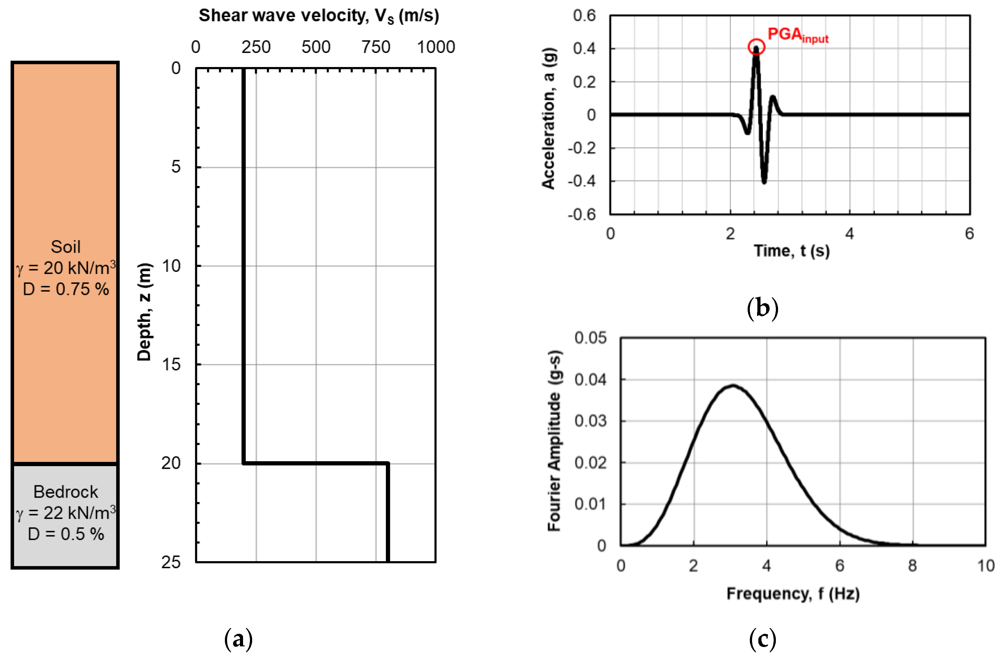
The considered ideal model consists of a 20 m column of homogeneous soil assumed with a linear visco-elastic behavior (Figure 1a).
The soil is characterized by a unit weight equal to 20 kN/m3 and a shear wave velocity, VS, equal to 200 m/s, constant with the depth. The dissipative behavior of the soil is described by a damping ratio, D, equal to 0.75%. This layer of deformable material overlying a rock half-space is assumed as a seismic bedrock, characterized by a unit weight equal to 22 kN/m3, a shear wave velocity, VS, equal to 800 m/s and a damping ratio equal to 0.5%.
The soil profile is subjected to an impulsive loading, similar to a Ricker-β wavelet type waveform, which is assumed to be recorded on a hypothetical rigid outcrop rock (outcrop motion), characterized by a Peak Ground Acceleration, PGA, equal at 0.4 g (Figure 1b) and centered on a frequency of about 3 Hz (Figure 1c), close to the natural frequency of vibration of the soil column, which is 2.5 Hz.
4. Numerical Model
Steps for defining the numerical model are detailed in the following subsections. The starting point is the identification of the analysis domain and discretization in subparts, depending on the soil properties and frequency content of the input motion [49]. Then, soil properties need to be defined, and the calculation of the initial effective stress state (static phase) is requested in some cases. Referring to the case of using codes based on 2D and 3D schemes, lateral boundary conditions need to be changed from static to dynamic phase to simulate the 1D propagation phenomena of S-waves. Finally, the input motion application is a function of the way the seismic bedrock is modeled, which can be deformable or rigid. In this latter hypothesis, the properties of the bedrock are not used in the analysis, but they are implicitly taken into account in the applied input motion [50,51].
The different steps are illustrated with specific application to the ideal profile of the previous Section 3, to better clarify any concept with a practical application.
4.1. Geometry and Discretization
One-dimensional SRA is based on the assumption that all boundaries are horizontal, and that the response of a soil deposit is predominantly caused by SH-waves propagating vertically from the underlying bedrock.
In one-dimensional ground response analysis, the soil is assumed to extend infinitely in the horizontal direction, while the bedrock is assumed to be a semi-infinite half-space. As a consequence, in the 1D codes, the definition of the geometric scheme is reduced to the identification of the deformable soil (i.e., depth of the seismic bedrock) and the discretization of the soil column in a finite number of sublayers. The maximum thickness of each sublayer is derived from the application of the [52] criterion. This criterion recommended that the minimum wavelength that propagates along the soil column should be discretized in at least 8 parts, to correctly track the horizontal displacements of the soil profile. The minimum wavelength is defined as the ratio between the shear wave velocity of the soil layer and the maximum frequency of the applied input motion. Assuming that the maximum frequency of the recorded seismic events is generally 25 Hz or less, and soft soils have a VS in the range 100 ÷ 200 m/s, the sublayer thickness consequently is usually adopted to be 0.5 or 1 m.
The considered 1D codes, except for EERA, can internally discretize the profile after the definition of the criteria; a manual operation is also allowed.
For the two-dimensional codes, QUAKE/W, FLAC, and PLAXIS, and the three-dimensional code, FLAC3D, it was necessary to define the dimensions of the analysis domain, depending on the choice to include (or not) the seismic bedrock.
Seismic Bedrock Modeling
The choice to model the seismic bedrock as rigid or deformable has a remarkable impact on the size of the analysis domain, boundary conditions at the base of the model and the type of input motion to apply [51,53]. The latter two will be discussed in Section 4.4 and Section 4.5, respectively.
In PLAXIS and QUAKE/W, only the column of 20 m of soil with a width of 3 m was modeled (Figure 2a). The considered width does not influence the result since proper boundary conditions were adopted (see Section 4.3). In this case, a rigid bedrock was assumed in the simulations.
On the other hand, in FLAC and FLAC3D, the analysis domain was extended to include the seismic bedrock. In this case, the bedrock deformability is directly modeled in the simulation. The usual practice suggests assigning a thickness of the bedrock of the same order of magnitude as the overlying deformable layer [50,54,55]. In the specific case, the analysis domain in FLAC has dimensions of 1 × 40 m and consists of 20 m of soil resting on 20 m of bedrock. Similarly, in FLAC3D, the dimensions are 1 × 1 × 40 m (Figure 2b).
For the two-dimensional codes, QUAKE/W, FLAC and PLAXIS, the analysis domain is discretized in elements, sometimes called zones, which are quadrangular for the first two codes and triangular for the last. In FLAC3D, rectangular parallelepipeds (brick elements) were used (Figure 2b). The grid of nodes and elements in which the analysis domain is divided is called mesh. The size of the mesh in the wave propagation direction should respect the criteria proposed by [52].
4.2. Soil Properties
For defining the properties of the materials, both formations have been schematized as homogeneous, isotropic materials with linear viscoelastic behavior. The soil parameters assumed in the model are the unit weight, γ, the velocity of propagation of the shear waves, VS and the damping ratio, D, as listed in Figure 1.
In the 1D codes, the bedrock was modeled as a deformable half-space; consequently, the shear modulus and the damping ratio of the seismic bedrock were introduced in the analysis. Similarly, for FLAC and FLAC3D, while in QUAKE/W and PLAXIS the properties of the bedrock are not used in the analysis, they are implicitly taken into account in the applied input motion (see Section 4.5).
For the two- and three-dimensional codes, the definition of the Poisson’s ratio, ν, is also required, which was assumed to be 0.45, close to the value assigned in the case of incompressible material.
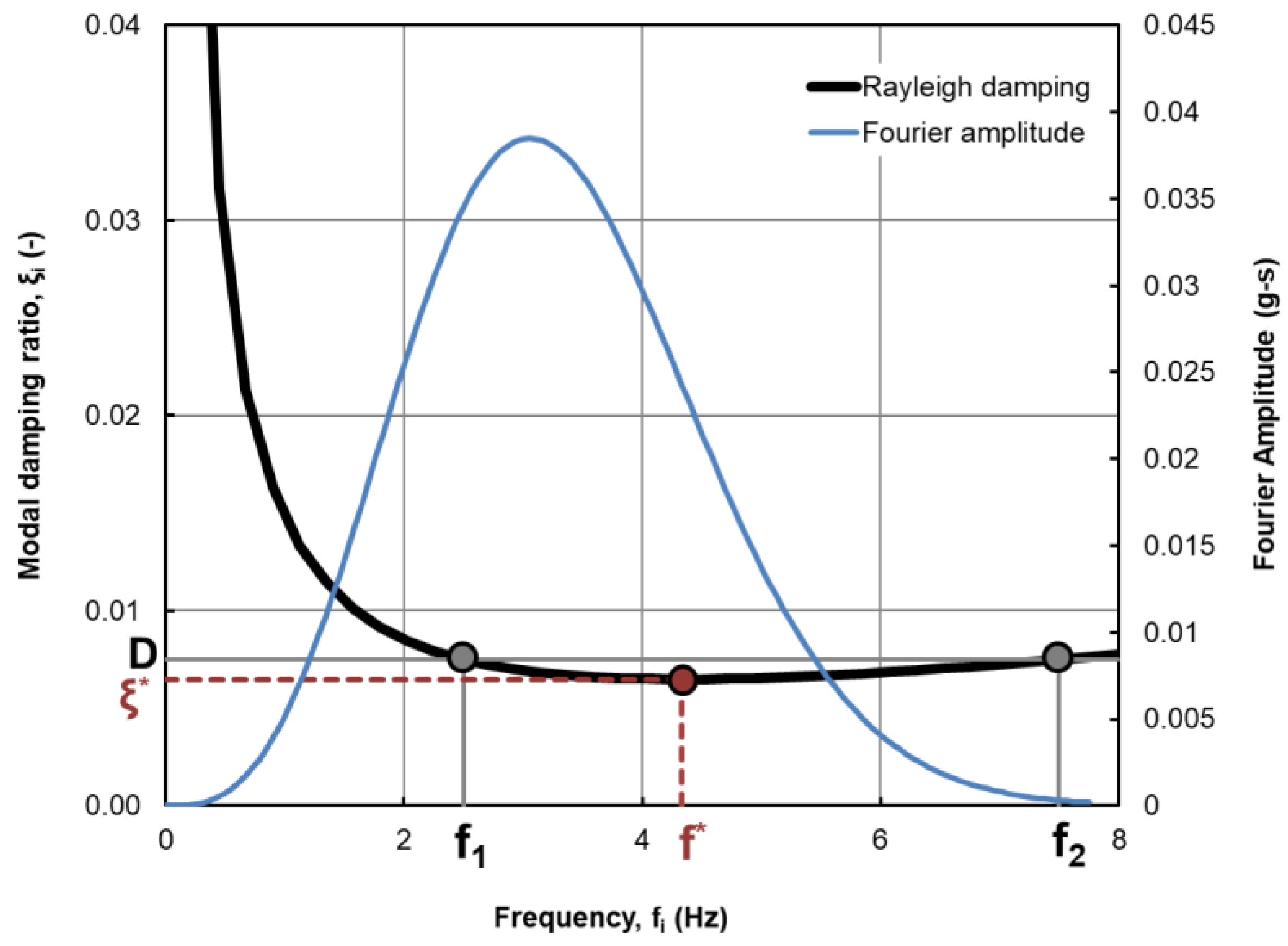
Rayleigh Damping Formulation
In computational codes that operate in the time domain, viscous damping needs to be assigned because the linear stress-strain relationship assumed for the soil produces shear stress-strain loops with no hysteretic damping.
The full Rayleigh damping formulation provides the viscous damping matrix as a result of the linear combination between the mass matrix and the stiffness matrix:
where α and β are the Rayleigh coefficients. [56,57] shows that the modal damping ratio, ξi, for the j-th mode is:
where fi is the frequency of the j-th mode. Figure 3 shows the Rayleigh damping curve expressed by Equation (2) overlapped to the Fourier amplitude spectrum of the considered motion.
[C] = α [M] + β [K]
Determination of the α and β coefficients can be obtained with two approaches, the first using a single control frequency, f*, and the second using two control frequencies, f1 and f2 [58,59].
The Rayleigh formulation is implemented according to a single frequency control approach in FLAC and FLAC3D, and according to a double frequency control approach in all the other non-linear codes.
The final goal in the definition of the Rayleigh damping curve is to set the viscous damping ratio as close as possible to the small strain damping ratio, D, of the soil.
In the double frequency control approach, the lower frequency, f1, is usually set equal to the natural vibration frequency of the soil column (2.5 Hz in this case), while the higher one, f2, is a multiplier of f1 [51]. In DEEPSOIL, a multiplier equal to 5 is recommended, while 3 is suggested in [12]. In SCOSSA, f2 is the multiplier of the natural frequency which rounds down the predominant frequency of the input motion. QUAKE/W computes the Rayleigh damping coefficients by using the lowest and the second-lowest frequencies of the soil column. In Cyclic1D, the α and β Rayleigh coefficients are denominated Am and Ak, respectively, to avoid confusion with some parameters of the adopted soil constitutive model. This code also allows the possibility to assign two different values of the damping ratio to the two control frequencies, called ξ1 and ξ2. Suggested values for ξ1 and ξ2 are between 0.2% and 20%.
In correspondence of the two control frequencies, f1 and f2, a damping ratio equal to the small strain damping ratio, D, of the soil is imposed (Figure 3). Consequently, by imposing these two conditions into Equation (2), the α and β Rayleigh coefficients can be obtained as:
In the single frequency approach, implemented in FLAC and FLAC3D, the minimum modal damping ratio, ξ*, of the Rayleigh curve and correspondent frequency, f*, need to be assigned. To use the same curve of Figure 3, the calculation of ξ* and f* can be still performed as a function of the two previously defined frequencies. In detail, by searching the minimum of the Rayleigh curve, dξ/df = 0, the f* value can be obtained, while ξ* can be then computed from Equation (2), as follows:
4.3. Lateral Boundary Conditions (2D and 3D Codes Only)
2D and 3D codes required the definition of the lateral boundary conditions. During the static phase, the displacements are prevented at the base in all the directions, while rollers that inhibit horizontal displacements are applied laterally. Static analysis was necessary to set the initial effective stress of the soil model. Moving from the static to the dynamic phase requires changing the boundary conditions.
Tie degree of freedom conditions in PLAXIS and free-field conditions in FLAC and FLAC3D were imposed along the domain boundaries to reproduce the one-dimensional propagation conditions, while in QUAKE/W vertical displacements were prevented during the dynamic phase of the analysis.
It should be pointed out that, if a 2D site condition is considered, the lateral outer boundaries of the numerical mesh should be placed far away from the area of interest [60]. Besides, the free-field condition is not applicable for axisymmetric geometry, and it can only be applied for a plane-strain or plane-stress analysis [61].
4.4. Boundary Conditions at the Base of the Model (2D and 3D Codes Only)
At the lower edge of the domain in FLAC and FLAC3D, absorbent barriers (quiet boundaries) have been applied, consisting of viscous dampers in both horizontal and vertical directions, able to simulate the presence of an elastic half-space.
In the other 2D codes, it is the case that of the models implemented in QUAKE/W and in PLAXIS, the displacements at the base of the soil column are prevented in both directions, indirectly modeling a rigid bedrock condition.
In the most recent versions of PLAXIS [25], it is also possible to consider the deformability of the bedrock by applying a “compliant base” option, but this possibility was not considered in this exercise.
4.5. Input Motion Application
In the 1D codes, a time history of acceleration was considered as reference input motion. The seismic bedrock was modeled as an elastic half-space and the “outcrop motion” [9,13,62] (Figure 1b and Figure 4) was applied at the base of the soil column. It is worth mentioning that a rigid bedrock can be also simulated in DEEPSOIL and SCOSSA. In this second case, it is necessary to consider the “inside motion”, sometimes expressed as “within motion”, which is the resulting motion between the wave train directed towards the surface and the train of the downward reflected wave. The inside motion implicitly considers the deformability of the bedrock since it is depending on both soil and bedrock properties. The inside motion of the considered input signal was obtained through the EERA code [19] in terms of the time history of acceleration. Figure 4 shows the differences between the outcrop and inside motion, which differ in terms of both PGA and the number of cycles. The acceleration time histories shown in the same figure refer to the analyzed case study.
Similarly, in FLAC and FLAC3D, the motion recorded on the outcropping rock (outcrop motion) was applied to the base of the model. Conversely to the 1D codes, the dynamic loading was applied to the base of the analysis domain as a temporal history of the shear stress [61], because, otherwise, the application in the same points of a time history of accelerations would have been nullified by the adsorbing quiet boundary. The applied shear stress time history depends on the bedrock properties and the upward propagating motion [50].
Conversely, in QUAKE/W and PLAXIS, the inside motion was applied at the base of the soil column since a rigid bedrock was considered in the model.
Even if it was not considered in this study, the possibility exists to model a rigid bedrock also in FLAC and FLAC3D. In this case, the bedrock is not modeled in the analysis domain and the time history of acceleration is applied at the base. Quiet boundaries cannot be adopted, but the vertical velocity at the base needs to be set to zero.
5. Results and Comparisons
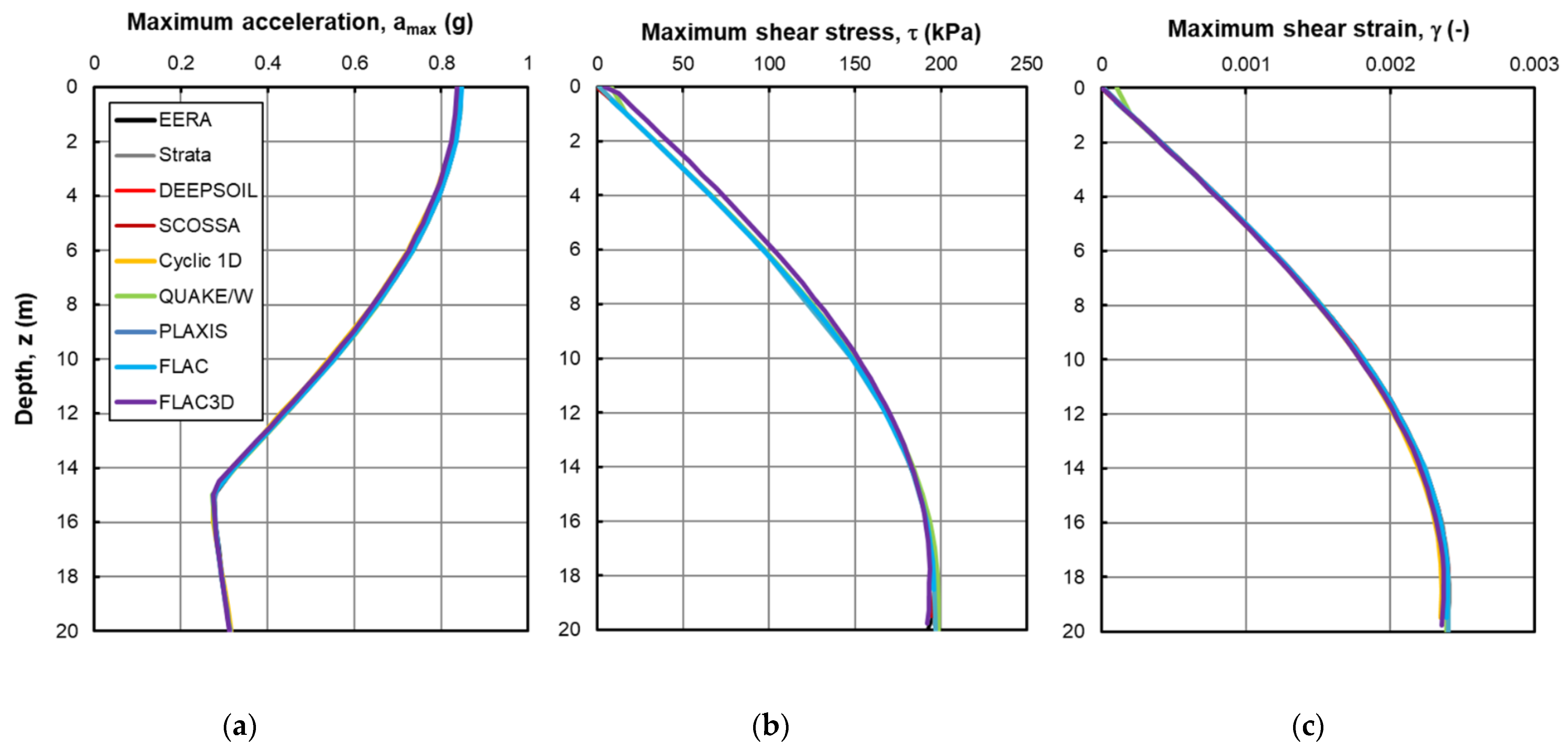
The comparison between the results of the simulations is expressed in terms of profiles of the maximum values of acceleration, shear stress and shear strain attained during the analyses (Figure 5), as well as in terms of the time history of acceleration at the ground level (Figure 6). As expected, when the initial and boundary conditions are correctly set, the results show that all codes lead to the same soil column response in terms of vertical profiles, with no appreciable differences (Figure 5). The maximum acceleration is attained at the surface with a mean predicted value of 0.843 g and a standard deviation of ±0.004 g. The maximum shear stress and strain are obtained at the base of the column, with a predicted value of 198.19 ± 9.79 kPa and 0.00239 ± 0.00002, respectively.
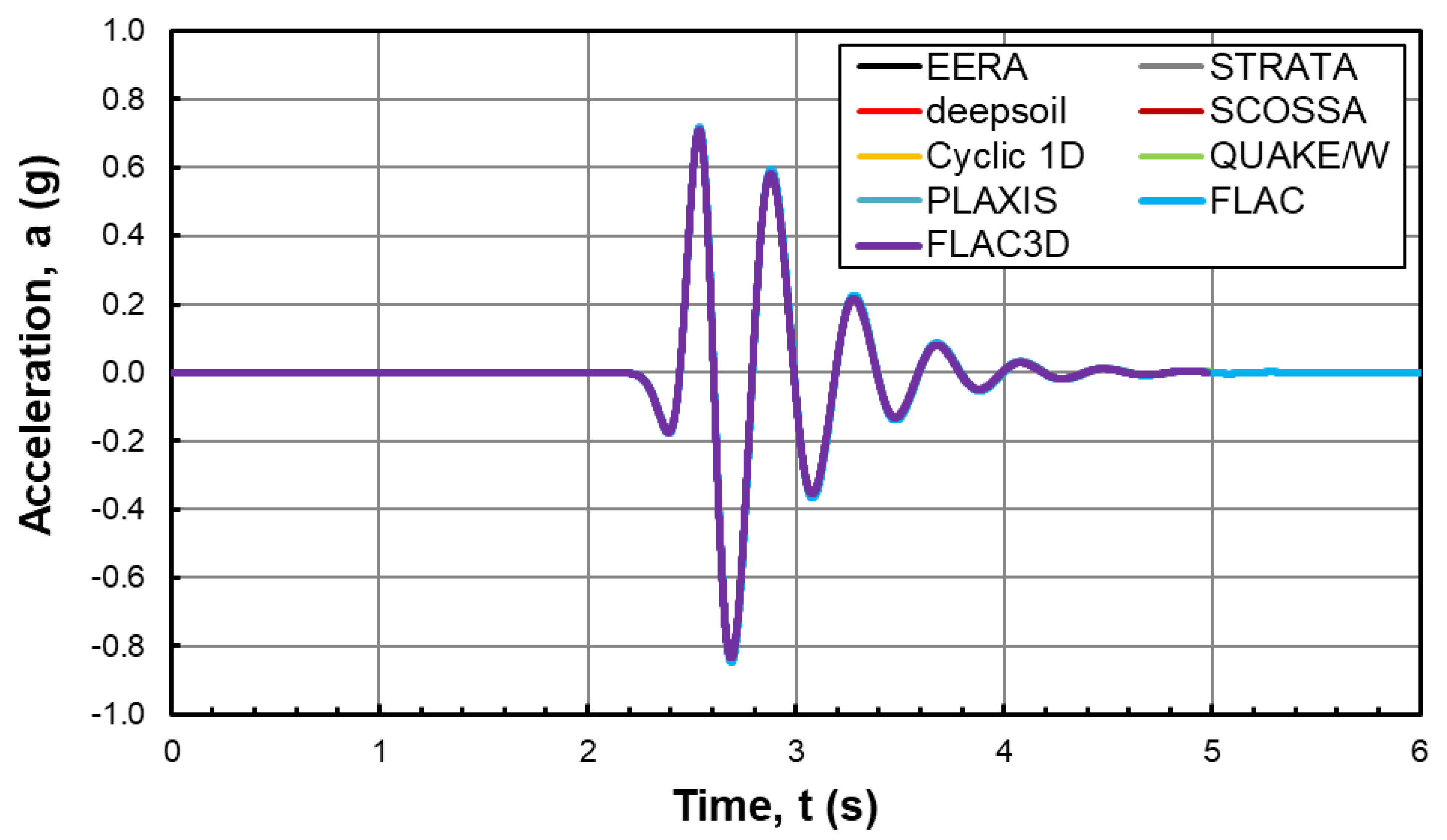
The time histories of the acceleration at the surface also show a perfect overlap among the different analyses (Figure 6). To obtain this, it was necessary to remove the time delay that the accelerogram resulting from the FLAC and FLAC3D analyses accumulated compared to the other time histories; this time delay is equal to the time that the wave needs to propagate along the 20 m of the seismic bedrock, i.e., for the base of the model to the roof of the bedrock (t = Hbedrock/VS, bed = 20 m/800 m/s = 0.025 s).
6. Discussion
The proposed ideal soil model is the simplest dynamic analysis that can be conceived. It can be used as the starting reference in many of the most complicated tasks. Just to provide some practical examples, it can be the benchmark to verify the capability of a calibrated advanced constitutive model to properly simulate soil behavior in the small strain range. Indeed, if the input motion (Figure 1b, Supplementary Material S1) is scaled to a low value of PGA (e.g., PGAinput = 0.05 g), a weak motion event can be defined. The response of a soil column modeled with an advanced constitutive model under the weak motion excitation should be still linear because the soil model is working in the small strain range. From a pragmatic perspective, the soil response should follow the results reported in Figure 7 (available in the Supplementary Material S2), where the accelerations are normalized to the PGA of the input, PGAinput (Figure 1b).
Another example of utility can be to reproduce the ideal model to properly set the boundary conditions in a new code or a code that someone is going to use for the first time. Especially for the input motion application and adsorbing boundaries, different codes have different options, so this is the simplest case to be used to check the rightness of the assumptions.
This simple exercise can be also considered as the first step of a series of comparisons moving from the elastic soil behavior, i.e., small-strain range, to the high non-linearity, i.e., high-strain range.
7. Conclusions
This study aimed to review the application of the boundary conditions and modeling of the initial small-strain soil behavior in some of the most popular computer codes adopted for SRA.
A checklist with all the steps to perform the analysis is provided and detailed for each of the nine computer codes considered in this review.
In this process, a critical point is represented by the modeling of the seismic bedrock and consequent input motion application. On one hand, the rigid model case has the great advantage to limit the analysis domain to analyze and consequently reducing the computation time [63,64]. On the other hand, the rigid bedrock requires an inside motion, rarely available (e.g., records of a downhole array), or not easy to define (e.g., deconvolution). The majority of the recorded seismic events are related to outcropping conditions (outcrop motion) because the recorded stations are largely located at the ground surface. In these cases, the deformability of the bedrock needs to be addressed.
Another critical aspect is usually constituted by the viscous damping modeled according to the Rayleigh formulation in many non-linear codes. A unified symbology has been used to describe the different approaches and provide a general framework for the definition of the input parameters.
Further steps in the analysis are the geometry, i.e., definition and discretization of the analysis domain, boundary condition and soil properties.
These initial steps in the simulation of the soil response under seismic conditions need to be carefully performed and checked to avoid inconsistencies and mistakes in the results. Therefore, this extremely simplified exercise constitutes the first step in the understanding and adequate learning of any calculation code for seismic response analysis. In this way, the illustrated case may be useful in the learning phase of new and/or more sophisticated computational codes for seismic response analysis in two- and three-dimensional conditions.
Finally, this review is considered a simple but powerful tool to contribute to the widespread of the basic concepts for SRA in routine professional applications.
Supplementary Materials
The following are available online at https://0-www-mdpi-com.brum.beds.ac.uk/article/10.3390/geosciences12020083/s1, Supplementary Material S1: Outcrop and inside input motion data: Input_motion.xlsx, Supplementary Material S2: Normalized_results.xlsx.
Funding
This research received no external funding.
Data Availability Statement
Further data presented in this study are available on request from the corresponding author.
Acknowledgments
The author was supported by the Italian Ministry of Research through the ‘Attraction and International Mobility’ project. The purchases of FLAC and FLAC3D Licenses were supported by the funds for large equipment of the University of L’Aquila. The author thanks the four anonymous reviewers for their comments and suggestions that greatly improved this manuscript.
Conflicts of Interest
The author declares no conflict of interest.
References
- Amorosi, A.; Boldini, D.; Di Lernia, A. Dynamic soil-structure interaction: A three-dimensional numerical approach and its application to the Lotung case study. Comput. Geotech. 2017, 90, 34–54. [Google Scholar] [CrossRef]
- Chiaradonna, A.; Bilotta, E.; d’Onofrio, A.; Flora, A.; Silvestri, F. A simplified procedure for evaluating post-seismic settlements in liquefiable soils. In Geotechnical Earthquake Engineering and Soil Dynamics V: Liquefaction Triggering, Consequences, and Mitigation; American Society of Civil Engineers: Reston, VA, USA, 2018; pp. 51–59. [Google Scholar]
- Chiaradonna, A.; d’Onofrio, A.; Bilotta, E. Assessment of post-liquefaction consolidation settlement. Bull. Earthq. Eng. 2019, 17, 5825–5848. [Google Scholar] [CrossRef]
- Alleanza, G.A.; d’Onofrio, A.; Silvestri, F.; Chiaradonna, A. Parametric study on 2D effect on the seismic response of alluvial valleys. In Earthquake Geotechnical Engineering for Protection and Development of Environment and Constructions; CRC Press: Boca Raton, FL, USA, 2019; pp. 1082–1089. ISBN 0429031270. [Google Scholar]
- Di Ludovico, M.; Chiaradonna, A.; Bilotta, E.; Flora, A.; Prota, A. Empirical damage and liquefaction fragility curves from 2012 Emilia earthquake data. Earthq. Spectra 2020, 36, 507–536. [Google Scholar] [CrossRef]
- Falcone, G.; Acunzo, G.; Mendicelli, A.; Mori, F.; Naso, G.; Peronace, E.; Porchia, A.; Romagnoli, G.; Tarquini, E.; Moscatelli, M. Seismic amplification maps of Italy based on site-specific microzonation dataset and one-dimensional numerical approach. Eng. Geol. 2021, 289, 106170. [Google Scholar] [CrossRef]
- Gruppo di Lavoro, M.S. Indirizzi e criteri per la microzonazione sismica. In Proceedings of the Conferenza Delle Regioni e Delle Provincie Autonome; Dipartimento Della protezione Civile: Roma, Italy, 2008; Volume 3. [Google Scholar]
- Moscatelli, M.; Albarello, D.; Scarascia Mugnozza, G.; Dolce, M. The Italian approach to seismic microzonation. Bull. Earthq. Eng. 2020, 18, 5425–5440. [Google Scholar] [CrossRef]
- Kramer, S.L. Geotechnical Earthquake Engineering; Pearson Education India: Noida, India, 1996; ISBN 8131707180. [Google Scholar]
- Mori, F.; Gena, A.; Mendicelli, A.; Naso, G.; Spina, D. Seismic emergency system evaluation: The role of seismic hazard and local effects. Eng. Geol. 2020, 270, 105587. [Google Scholar] [CrossRef]
- Stewart, J.P. Benchmarking of Nonlinear Geotechnical Ground Response Analysis Procedures; Pacific Earthquake Engineering Research Center: Berkeley, CA, USA, 2008. [Google Scholar]
- Kwok, A.O.L.; Stewart, J.P.; Hashash, Y.M.A.; Matasovic, N.; Pyke, R.; Wang, Z.; Yang, Z. Use of exact solutions of wave propagation problems to guide implementation of nonlinear seismic ground response analysis procedures. J. Geotech. Geoenviron. Eng. 2007, 133, 1385–1398. [Google Scholar] [CrossRef] [Green Version]
- Régnier, J.; Bonilla, L.; Bard, P.; Bertrand, E.; Hollender, F.; Kawase, H.; Sicilia, D.; Arduino, P.; Amorosi, A.; Asimaki, D.; et al. PRENOLIN: International Benchmark on 1D Nonlinear Site-Response Analysis—Validation Phase Exercise. Bull. Seismol. Soc. Am. 2018, 108, 876–900. [Google Scholar] [CrossRef]
- Kaklamanos, J.; Baise, L.G.; Thompson, E.M.; Dorfmann, L. Comparison of 1D linear, equivalent-linear, and nonlinear site response models at six KiK-net validation sites. Soil Dyn. Earthq. Eng. 2015, 69, 207–219. [Google Scholar] [CrossRef]
- Kaklamanos, J.; Bradley, B.A.; Thompson, E.M.; Baise, L.G. Critical parameters affecting bias and variability in site-response analyses using KiK-net downhole array data. Bull. Seismol. Soc. Am. 2013, 103, 1733–1749. [Google Scholar] [CrossRef]
- Tropeano, G.; Chiaradonna, A.; d’Onofrio, A.; Silvestri, F. A numerical model for non-linear coupled analysis of the seismic response of liquefiable soils. Comput. Geotech. 2019, 105, 211–227. [Google Scholar] [CrossRef]
- Chiaradonna, A.; D’onofrio, A.; Silvestri, F.; Tropeano, G. Prediction of non-linear soil behaviour in saturated sand: A loosely coupled approach for 1d effective stress analysis. In Proceedings of the 7th International Conference on Earthquake Geotechnical Engineering, ICEGE 2019; CRC Press/Balkema: Boca Raton, FL, USA, 2019; pp. 1746–1753. [Google Scholar]
- Amorosi, A.; Boldini, D.; Elia, G. Parametric study on seismic ground response by finite element modelling. Comput. Geotech. 2010, 37, 515–528. [Google Scholar] [CrossRef]
- Bardet, J.P.; Ichii, K.; Lin, C.H. EERA: A Computer Program for Equivalent-Linear Earthquake Site Response Analyses of Layered Soil; University of Southern California: Los Angeles, CA, USA, 2000; p. 40. [Google Scholar]
- Kottke, A.R.; Wang, X.; Rathje, E.M. Strata Technical Manual. 2019. Available online: https://github.com/arkottke/strata (accessed on 23 December 2021).
- Hashash, Y.M.A.; Musgrove, M.; Harmon, J.; Ilhan, O.; Xing, G.; Numanoglu, O.; Groholski, D.R.; Phillips, C.A.; Park, D. Deepsoil Version 7.0; University of Illinois at Urbana-Champaign: Urbana, IL, USA, 2020; pp. 1–170. [Google Scholar]
- Tropeano, G.; Chiaradonna, A.; d’Onofrio, A.; Silvestri, F. An innovative computer code for 1D seismic response analysis including shear strength of soils. Geotechnique 2016, 66, 95–105. [Google Scholar] [CrossRef]
- Elgamal, A.; Yang, Z.; Lu, J. Cyclic 1D Seismic Ground Response Version 1.4 User’s Manual; University of California: San Diego, CA, USA, 2015; pp. 1–28. [Google Scholar]
- Dynamic Modeling with QUAKE/W; Geo-Slope International Ltd.: Calgary, AB, Canada, 2014; pp. 1–173.
- PLAXIS bv PLAXIS CONNECT Edition V21.01 General Information Manual. 2021. Available online: https://communities.bentley.com/products/geotech-analysis/w/plaxis-soilvision-wiki/50826/manuals-archive---plaxis (accessed on 23 December 2021).
- FLAC-Fast Lagrangian Analysis of Continua. User’s Guide; Itasca Consulting Group, Inc.: Minneapolis, MN, USA, 2021.
- FLAC3D-Fast Lagrangian Analysis of Continua in 3 Dimensions. User’s Guide; Itasca Consulting Group, Inc.: Minneapolis, MN, USA, 2021.
- Groholski, D.R.; Hashash, Y.M.A.; Matasovic, N. Learning of pore pressure response and dynamic soil behavior from downhole array measurements. Soil Dyn. Earthq. Eng. 2014, 61–62, 40–56. [Google Scholar] [CrossRef]
- Olson, S.M.; Mei, X.; Hashash, Y.M.A. Nonlinear site response analysis with pore-water pressure generation for liquefaction triggering evaluation. J. Geotech. Geoenviron. Eng. 2020, 146, 4019128. [Google Scholar] [CrossRef]
- Chiaradonna, A.; Flora, A.; d’Onofrio, A.; Bilotta, E. A pore water pressure model calibration based on in-situ test results. Soils Found. 2020, 60, 327–341. [Google Scholar] [CrossRef]
- Chiaradonna, A.; Tropeano, G.; d’Onofrio, A.; Silvestri, F. Development of a simplified model for pore water pressure build-up induced by cyclic loading. Bull. Earthq. Eng. 2018, 16, 3627–3652. [Google Scholar] [CrossRef]
- Chiaradonna, A.; Tropeano, G.; d’Onofrio, A.; Silvestri, F. A Simplified Method for Pore Pressure Buildup Prediction: From Laboratory Cyclic Tests to the 1D Soil Response Analysis in Effective Stress Conditions. Procedia Eng. 2016, 158, 302–307. [Google Scholar] [CrossRef]
- Yang, Z.; Lu, J.; Elgamal, A. A web-based platform for computer simulation of seismic ground response. Adv. Eng. Softw. 2004, 35, 249–259. [Google Scholar] [CrossRef]
- Lu, J.; Elgamal, A.-W.M.; Yang, Z. Cyclic1D: A Computer Program for Seismic Ground Response; Department of Structural Engineering, University of California: San Diego, CA, USA, 2006. [Google Scholar]
- Stability Modeling with Slope/W; Geo-Slope International Ltd.: Calgary, AB, Canada, 2012.
- Seepage Modeling with SEEP/W; Geo-Slope International Ltd.: Calgary, AB, Canada, 2012; p. 307.
- Martin, G.R.; Seed, H.B.; Finn, W.D.L. Fundamentals of liquefaction under cyclic loading. J. Geotech. Eng. Div. 1975, 101, 423–438. [Google Scholar] [CrossRef]
- Schanz, T.; Vermeer, P.A.; Bonnier, P.G. The hardening soil model: Formulation and verification. In Beyond 2000 in Computational Geotechnics; Routledge: London, UK, 2019; pp. 281–296. ISBN 1315138204. [Google Scholar]
- Boulanger, R.W.; Ziotopoulou, K. PM4Sand (Version 3): A Sand Plasticity Model for Earthquake Engineering Applications; University of California: Davis, CA, USA, 2015. [Google Scholar]
- Petalas, A. PLAXIS Liquefaction Model UBC3D-PLM, 2013. Available online: https://communities.bentley.com/cfs-file/__key/communityserver-wikis-components-files/00-00-00-05-58/UBC3D_2D00_PLM_2D00_REPORT.June2013.pdf (accessed on 23 December 2021).
- Byrne, P.M. A Cyclic Shear-Volume Coupling and Pore Pressure Model for Sand; Missouri University of Science and Technology: Rolla, MO, USA, 1991. [Google Scholar]
- Boulanger, R.W.; Ziotopoulou, K. PM4Silt (Version 1): A Silt Plasticity Model for Earthquake Engineering Applications; University of California: Davis, CA, USA, 2018. [Google Scholar]
- Andrianopoulos, K.I.; Papadimitriou, A.G.; Bouckovalas, G.D. Explicit integration of bounding surface model for the analysis of earthquake soil liquefaction. Int. J. Numer. Anal. Methods Geomech. 2010, 34, 1586–1614. [Google Scholar] [CrossRef]
- Andrianopoulos, K.I.; Papadimitriou, A.G.; Bouckovalas, G.D. Bounding surface plasticity model for the seismic liquefaction analysis of geostructures. Soil Dyn. Earthq. Eng. 2010, 30, 895–911. [Google Scholar] [CrossRef]
- Itasca Consulting Group. User Defined Model-UDM. Available online: https://www.itascacg.com/software/udm-library?software=flac&category=&phrase= (accessed on 23 December 2021).
- Cheng, Z. Application of SANISAND Dafalias-Manzari model in FLAC 3D. In Continuum and Distinct Element Numerical Modeling in Geomechanics; Itasca International Inc.: Minneapolis, MN, USA, 2013. [Google Scholar]
- Dafalias, Y.F.; Manzari, M.T. Simple plasticity sand model accounting for fabric change effects. J. Eng. Mech. 2004, 130, 622–634. [Google Scholar] [CrossRef]
- Wang, R.; Zhang, J.; Wang, G. Computers and Geotechnics A unified plasticity model for large post-liquefaction shear deformation of sand. Comput. Geotech. 2014, 59, 54–66. [Google Scholar] [CrossRef]
- Bathe, K.-J. Finite Element Procedures; Prentice Hall: Hoboken, NJ, USA, 2006; ISBN 097900490X. [Google Scholar]
- Mejia, L.H.; Dawson, E.M. Earthquake deconvolution for FLAC. In Proceedings of the 4th International FLAC Symposium on Numerical Modeling in Geomechanics; Citeseer: Princeton, NJ, USA, 2006; pp. 4–10. [Google Scholar]
- Falcone, G.; Naso, G.; Mori, F.; Mendicelli, A.; Acunzo, G.; Peronace, E.; Moscatelli, M. Effect of Base Conditions in One-Dimensional Numerical Simulation of Seismic Site Response: A Technical Note for Best Practice. GeoHazards 2021, 2, 430–441. [Google Scholar] [CrossRef]
- Kuhlemeyer, R.L.; Lysmer, J. Finite Element Method Accuracy for Wave Propagation Problems. J. Soil Mech. Found. Div. 1973, 99, 421–427. [Google Scholar] [CrossRef]
- Falcone, G.; Romagnoli, G.; Naso, G.; Mori, F.; Moscatelli, M.; Peronace, E. Effect of bedrock stiffness and thickness on numerical simulation of seismic site response. Italian case studies. Soil Dyn. Earthq. Eng. 2020, 139, 106361. [Google Scholar] [CrossRef]
- Boulanger, R.W.; Montgomery, J. Nonlinear deformation analyses of an embankment dam on a spatially variable liquefiable deposit. Soil Dyn. Earthq. Eng. 2016, 91, 222–233. [Google Scholar] [CrossRef]
- Paull, N.A.; Boulanger, R.W.; DeJong, J.T. Accounting for spatial variability in nonlinear dynamic analyses of embankment dams on liquefiable deposits. J. Geotech. Geoenviron. Eng. 2020, 146, 4020124. [Google Scholar] [CrossRef]
- Chopra, A.K. Dynamics of Structures; Pearson Education India: Noida, India, 2007; ISBN 8131713296. [Google Scholar]
- Zienkiewicz, O.C.; Taylor, R.L.; Zhu, J.Z. The Finite Element Method: Its Basis and Fundamentals; Elsevier: Amsterdam, The Netherlands, 2005; ISBN 008047277X. [Google Scholar]
- Verrucci, L.; Pagliaroli, A.; Lanzo, G.; Di Buccio, F.; Biasco, A.P.; Cucci, C. Damping formulations for finite difference linear dynamic analyses: Performance and practical recommendations. Comput. Geotech. 2022, 142, 104568. [Google Scholar] [CrossRef]
- Lanzo, G.; Pagliaroli, A.; D’Elia, B. Numerical Study on the Frequency-Dependent Viscous Damping in Dynamic Response Analyses of Ground; Earthquake Resistant Engineering Structures IV; WIT Press: Boston, MA, USA, 2003; pp. 315–324. [Google Scholar]
- Bassal, P.C.; Boulanger, R.W. System Response of an Interlayered Deposit with Spatially Preferential Liquefaction Manifestations. J. Geotech. Geoenviron. Eng. 2021, 147, 1–23. [Google Scholar] [CrossRef]
- LAC-Fast Lagrangian Analysis of Continua. Online Manual Table of Contents. Dynamic Analysis; Itasca Consulting Group, Inc.: Minneapolis, MN, USA, 2021.
- Régnier, J.; Bonilla, L.F.; Bard, P.Y.; Bertrand, E.; Hollender, F.; Kawase, H.; Sicilia, D.; Arduino, P.; Amorosi, A.; Asimaki, D.; et al. International benchmark on numerical simulations for 1D, nonlinear site response (Prenolin): Verification phase based on canonical cases. Bull. Seismol. Soc. Am. 2016, 106, 2112–2135. [Google Scholar] [CrossRef]
- Chiaradonna, A.; Tropeano, G.; d’Onofrio, A.; Silvestri, F. Interpreting the deformation phenomena of a levee damaged during the 2012 Emilia earthquake. Soil Dyn. Earthq. Eng. 2019, 124, 389–398. [Google Scholar] [CrossRef]
- Chiaradonna, A.; Lirer, S.; Flora, A. A liquefaction potential integral index based on pore pressure build-up. Eng. Geol. 2020, 272, 105620. [Google Scholar] [CrossRef]
Figure 1.
The ideal case considered in the analysis: Soil stratigraphy and shear wave velocity as a function of the depth (a); Reference seismic input on outcropping rock in terms of the time history of acceleration (the PGA attained is highlighted with a symbol) (b) and the Fourier amplitude spectrum (c).

Figure 2.
Geometry and mesh of the analysis domain adopted in the code: (a) QUAKE/W (the triangles along the boundaries of the soil identify the constraints applied during the static phase) and (b) FLAC3D (the soil has a tight mesh compared to the coarse mesh of the bedrock).
Figure 2.
Geometry and mesh of the analysis domain adopted in the code: (a) QUAKE/W (the triangles along the boundaries of the soil identify the constraints applied during the static phase) and (b) FLAC3D (the soil has a tight mesh compared to the coarse mesh of the bedrock).

Figure 3.
Rayleigh damping curve (black line) over imposed to the Fourier amplitude spectrum with the identification of the single control frequency, f*, the two control frequencies, f1, and f2, the minimum modal damping ratio, ξ*, and the small strain damping ratio, D.
Figure 3.
Rayleigh damping curve (black line) over imposed to the Fourier amplitude spectrum with the identification of the single control frequency, f*, the two control frequencies, f1, and f2, the minimum modal damping ratio, ξ*, and the small strain damping ratio, D.

Figure 4.
Reference sketch for the definition of the input seismic motion: ‘outcrop motion’ of the outcropping rock and ‘inside motion’ at the interface between the rock bedrock and the deformable soil deposit. The time histories of acceleration show the outcrop and inside motions of the considered ideal case (PGA highlighted with a symbol), both available in the Supplementary Material S1.

Figure 5.
Vertical profiles of the maximum acceleration (a), shear stress (b), and shear strain (c) deriving from the analyzes carried out with the nine considered codes.
Figure 5.
Vertical profiles of the maximum acceleration (a), shear stress (b), and shear strain (c) deriving from the analyzes carried out with the nine considered codes.

Figure 6.
Temporal histories of the acceleration predicted at the surface of the soil column from the analyzes carried out with the nine considered codes.
Figure 6.
Temporal histories of the acceleration predicted at the surface of the soil column from the analyzes carried out with the nine considered codes.

Figure 7.
Normalized results: (a) profile of maximum acceleration as a function of the depth and (b) time history of acceleration at the ground level both normalized to the PGA of the input motion, PGAinput (available in the Supplementary Material S2).
Figure 7.
Normalized results: (a) profile of maximum acceleration as a function of the depth and (b) time history of acceleration at the ground level both normalized to the PGA of the input motion, PGAinput (available in the Supplementary Material S2).


Table 1.
Adopted computer codes and related capabilities for seismic response analysis.
| Geometry | Code | Reference | Total Stress | Effective Stress | ||
|---|---|---|---|---|---|---|
| Equivalent Linear | Non- Linear | Loosely Coupled | Fully Coupled | |||
| 1D | EERA | [19] | X | |||
| Strata | [20] | X | ||||
| DEEPSOIL | [21] | X | X | X | ||
| SCOSSA | [16,22] | X | X | |||
| Cyclic1D | [23] | X | ||||
| 2D | Quake/W | [24] | X | X | X | |
| PLAXIS | [25] | X | X | |||
| FLAC | [26] | X | X | X | ||
| 3D | FLAC3D | [27] | X | X | X | |
Table 2.
Parameters of the Rayleigh damping with identification of the input variables requested by the different non-linear codes.
Table 2.
Parameters of the Rayleigh damping with identification of the input variables requested by the different non-linear codes.
| Non-Linear Code | α | β | D (-) | f1 (Hz) | f2 (Hz) | ξ* (-) | f* (Hz) |
|---|---|---|---|---|---|---|---|
| 0.17671 | 0.00024 | 0.0075 | 2.5 | 7.5 | 0.0065 | 4.33 | |
| DEEPSOIL | X | X | X | ||||
| SCOSSA | X | X | X | ||||
| Cyclic1D | X | X | X * | X * | X * | ||
| Quake/W | X | X | X | ||||
| PLAXIS | X | X | X * | X * | X * | ||
| FLAC | X | X | |||||
| FLAC3D | X | X |
* These parameters can be introduced alternatively to α and β.
Publisher’s Note: MDPI stays neutral with regard to jurisdictional claims in published maps and institutional affiliations. |
© 2022 by the author. Licensee MDPI, Basel, Switzerland. This article is an open access article distributed under the terms and conditions of the Creative Commons Attribution (CC BY) license (https://creativecommons.org/licenses/by/4.0/).
Share and Cite
MDPI and ACS Style
Chiaradonna, A. Defining the Boundary Conditions for Seismic Response Analysis—A Practical Review of Some Widely-Used Codes. Geosciences 2022, 12, 83. https://0-doi-org.brum.beds.ac.uk/10.3390/geosciences12020083
AMA Style
Chiaradonna A. Defining the Boundary Conditions for Seismic Response Analysis—A Practical Review of Some Widely-Used Codes. Geosciences. 2022; 12(2):83. https://0-doi-org.brum.beds.ac.uk/10.3390/geosciences12020083
Chicago/Turabian StyleChiaradonna, Anna. 2022. "Defining the Boundary Conditions for Seismic Response Analysis—A Practical Review of Some Widely-Used Codes" Geosciences 12, no. 2: 83. https://0-doi-org.brum.beds.ac.uk/10.3390/geosciences12020083
Note that from the first issue of 2016, this journal uses article numbers instead of page numbers. See further details here.