Article

OpenMetBuoy-v2021: An Easy-to-Build, Affordable, Customizable, Open-Source Instrument for Oceanographic Measurements of Drift and Waves in Sea Ice and the Open Ocean

by
Jean Rabault
1,*,
Takehiko Nose
2,
Gaute Hope
1,
Malte Müller
1,3,
Øyvind Breivik
1,
Joey Voermans
4,
Lars Robert Hole
1,
Patrik Bohlinger
1,
Takuji Waseda
2,5,
Tsubasa Kodaira
2,
Tomotaka Katsuno
2,
Mark Johnson
6,
Graig Sutherland
7,
Malin Johansson
8,
Kai Haakon Christensen
1,
Adam Garbo
9,
Atle Jensen
3,
Olav Gundersen
3,
Aleksey Marchenko
10 and
Alexander Babanin
4
1
Norwegian Meteorological Institute, 0313 Oslo, Norway
2
Graduate School of Frontier Sciences, The University of Tokyo, Kashiwa 277-8561, Japan
3
Department of Mathematics, University of Oslo, 0313 Oslo, Norway
4
Department of Infrastructure Engineering, The University of Melbourne, Parkville, VIC 3052, Australia
5
Japan Agency for Marine-Earth Science and Technology, Yokosuka 237-0061, Japan
6
College of Fisheries and Ocean Science, The University of Alaska Fairbanks, Fairbanks, AK 99775, USA
7
Environment Climate Change Canada, Environmental Numerical Prediction Research, Dorval, QC H9P 1J3, Canada
8
Department of Physics and Technology, UiT The Arctic University of Norway, 9037 Tromsø, Norway
9
Water and Ice Research Laboratory, Carleton University, Ottawa, ON K1S 5B6, Canada
10
Department of Arctic Technology, The University Center in Svalbard, P.O. Box 156, 9171 Longyearbyen, Norway
*
Author to whom correspondence should be addressed.
Submission received: 22 January 2022 / Revised: 14 February 2022 / Accepted: 22 February 2022 / Published: 26 February 2022

Abstract

:
There is a wide consensus within the polar science, meteorology, and oceanography communities that more in situ observations of the ocean, atmosphere, and sea ice are required to further improve operational forecasting model skills. Traditionally, the volume of such measurements has been limited by the high cost of commercially available instruments. An increasingly attractive solution to this cost issue is to use instruments produced in-house from open-source hardware, firmware, and postprocessing building blocks. In the present work, we release the next iteration of our open-source drifter and wave-monitoring instrument, which follows these solution aspects. The new design is significantly less expensive (typically by a factor of 5 compared with our previous, already cost-effective instrument), much easier to build and assemble for people without specific microelectronics and programming competence, more easily extendable and customizable, and two orders of magnitude more power-efficient (to the point where solar panels are no longer needed even for long-term deployments). Improving performance and reducing noise levels and costs compared with our previous generation of instruments is possible in large part thanks to progress from the electronics component industry. As a result, we believe that this will allow scientists in geosciences to increase by an order of magnitude the amount of in situ data they can collect under a constant instrumentation budget. In the following, we offer (1) a detailed overview of our hardware and software solution, (2) in situ validation and benchmarking of our instrument, (3) a fully open-source release of both hardware and software blueprints. We hope that this work, and the associated open-source release, will be a milestone that will allow our scientific fields to transition towards open-source, community-driven instrumentation. We believe that this could have a considerable impact on many fields by making in situ instrumentation at least an order of magnitude less expensive and more customizable than it has been for the last 50 years, marking the start of a new paradigm in oceanography and polar science, where instrumentation is an inexpensive commodity and in situ data are easier and less expensive to collect.

1. Introduction

Our inability to accurately capture climatological changes of sea ice in the polar seas has created renewed interest in the dynamic interaction between sea ice and waves. This has resulted in the last few years in a number of studies that investigate the coupling between sea ice and the ocean through theoretical considerations [1,2,3,4,5,6,7], laboratory experiments [8,9,10,11,12], and field experiments [13,14,15,16,17,18,19,20,21,22,23,24]. Despite the advances that these studies bring, there is a growing consensus that further progress in the field can only be achieved through the collection of more observations of waves in ice. In particular, phenomena related to floe size distribution [4,25,26,27], energy dissipation due to turbulence and collisions [28,29,30,31], and sea ice breakup [32,33,34,35] are still imperfectly modeled and understood, and advancing the state-of-the-art would require additional direct observations from the ice.
Unfortunately, one faces a number of challenges in reproducing the complexity of wave–ice interaction either in experiments (due to, for example, scaling issues [9], and the diversity and realism of sea ice conditions that can be obtained in the laboratory compared with the field [12]), or in models (there, also, due to the complexity and multiscale properties of waves in ice and ice floe size distribution [36,37]). Arguably, the current state of the art in wave–ice interaction parametrization and modeling consists of a variety of (involved and mathematically advanced) models whose formulations are relatively loosely based on some specific archetypical sea ice conditions and the associated physical mechanisms, with a number of “tuning parameters” that are empirically fitted to experimental or laboratory data [38,39]. This approach is quite ad hoc and brittle, which is in stark contrast with the importance of waves in ice and their impact on both weather and climate.
As a consequence, having access to large datasets of high temporal and spatial resolution direct observations of waves in ice is a key ingredient to improving both small scale wave–ice interaction parametrization, large-scale coupled wave–ice models, and our understanding of the weather and climate dynamics in the polar regions. There are a number of recent works that highlight the importance of the volume of such datasets for unveiling wave–ice interaction mechanisms. For example, Voermans et al. [14] showed that wave conditions that result in sea ice breakup events can be quite accurately described with a simple threshold mechanism, but in order to be able to observe such a threshold, a relatively large aggregated dataset is necessary.
There are relatively few methods available for measuring waves in ice. The most common and established method considers the deployment of instrumentation in situ, providing surface truth of the sea ice motion under the influence of waves. Such instruments typically use either an Inertial Motion Unit (IMU, i.e., a combination of accelerometer, gyroscope, and magnetometer, together with some data fusion processing, e.g., Kohout et al. [40], Rabault et al. [41]), or a high-accuracy GPS [42,43] to measure the sea ice motion and compute wave spectra. Less common techniques are using pressure sensors to measure the wave-induced pressure fluctuation to derive wave observations [23]. Remote sensing is a promising avenue to obtain observations of waves in ice across large spatial scales [44,45] to a far larger extent compared with what can be achieved using in situ instrumentation, though the number of wave parameters that can be retrieved and the accuracy that can be achieved is still limited and a topic for open research. Moreover, remote sensing requires considerably more in situ observations for calibration and validation. As a consequence, the most-established and accurate method today is still to deploy instrumentation in situ to measure waves in ice.
Performing in situ measurements of waves in ice is, however, a challenging and costly operation. Commercial instruments have traditionally been extremely expensive, and sometimes of varying quality, with typical prices after taxes in the 7.5–50 kUSD range. The situation became somewhat better with the emergence of new actors, such as Sofar and their Spotter buoy [46], which took down the price to a typical 6–8 kUSD cost per instrument, once import taxes and satellite communication fees were factored in. Still, the Sofar Spotter, while gaining from being a very modern as well as relatively low-cost design, is not very well-adapted for use in the polar regions, as it was designed primarily for measuring open water wave statistics and, correspondingly, relatively large waves. In particular, its battery life limits the duration of deployments in the polar night [43]. In addition, its GPS-based wave measurement method, while having many advantages in open water (such as accurate directional wave spectrum measurement), has significantly higher noise for the typically small waves observed in the ice than what can be achieved with a modern Inertial Motion Unit (IMU).
As a consequence of these challenges, a number of groups have developed in-house, custom instrumentation for measurements of waves in ice (e.g., [40,41,47]. A very brief overview is provided in Figure 1. This is, in our opinion, a situation that is so far quite inefficient. Indeed, a number of groups develop their own closed-source solution, in parallel of each other, wasting a large amount of engineering resources in the form of working hours and prototyping costs in the process.
An increasingly promising direction is the development of open-source instrumentation, which allows to both reduce hardware costs and mutualize the instrumentation development workload. This approach was recently adopted by Rabault et al. [51] and, since its development in 2015, has undergone several updates (the full lineage of our series of open-source instruments is presented in Figure 2). In the following, we will refer to the design described in Rabault et al. [51] as the “v2018 instrument” or “v2018” in short. Since the initial deployment of the first v2018 instruments Rabault et al. [51], the low-cost and open-source fundament of the instrument has promoted usage and international collaboration across the world. The v2018, and adaptations thereof, have been deployed in both the Arctic and Antarctic to study sea-ice drift [52], wave attenuation and dispersion [19], and wave-induced sea ice break-up [14]. Through these collaborations and technological advancements, points of improvement were identified, which supported advancement of the v2018 and development of the latest “v2021” version.
These challenges of high instrumentation costs and the need for more in situ ground truth data are not specific to the waves in ice community. Similarly, the rise of low-cost (and possibly open-source) electronics is an evolution that is increasingly attracting the attention of both research groups and public agencies across the world. For example, this trend can be identified also in the technical development and history of the “Swift drifters” family, among others, which are also advancing towards open-source, low-cost, “do it yourself” technical solutions [53,54,55], focusing on measuring waves in the open ocean. Another example of this trend is visible in recent works that focus on building small, inexpensive, biodegradable surface drifters [46]. Similarly, the Defense Advanced Research Projects Agency (DARPA) is actively pursuing similar efforts with its “Ocean of Things” project [56], which aims at “deploying thousands of low-cost, environmentally friendly, intelligent floats that drift as a distributed sensor network” (quote from the Ocean of Things project webpage, accessed December 2021).
This paper is organized as follows. First, we discuss the general design and features of the instrument v2021. Then, we present a detailed validation of the instrument v2021: (i) in a preliminary deployment, aimed at validating the general concept of the instrument and the power efficiency of the design; (ii) in laboratory experiments that tested the noise threshold of the waves measurements; (iii) in a full-scale deployment in the Russian Arctic; (iv) in a full-scale deployment in the Caribbean. Finally, we offer a few words of conclusion and present a road map for future development. All hardware blueprints, embedded software, postprocessing codes, and detailed instructions are released as open source on Github, as indicated in the Appendix A.

2. General Design and Features of the Instrument v2021

2.1. Microcontroller

Unlike the instrument v2018, and unlike all other wave-measuring instruments that we are aware of, the v2021 is based solely on a high-performance microcontroller for performing both data acquisition and in situ data processing. This is a major shift from previous designs, which usually resorted to some sort of embedded microcomputer for performing the computation of wave spectra (typical previous solutions, such as those based on a Raspberry Pi, run a stripped down version of Linux or Windows), with the measurements themselves being performed either by the same microcomputer, or by a separate, lower power microcontroller. This traditional approach has a dramatic effect on power consumption. A typical microcomputer consumes around 1 to 2 W (for example, the Raspberry Pi used in the v2018 consumes typically up to around 350 mA while running at 5 V), while a modern microcontroller can consume as little as 1 to 2 mW (the microcontroller used in the v2021 consumes typically 500 μ A while running at a 3.3 V voltage). This factor 1000 in power efficiency allows for significant simplifications and flexibility in the instrument design. This is of particular importance to instrument performance in the polar regions where the battery is generally the main limiting factor in the field experiment duration. In addition, microcomputers rely on a complete operating system for running their workloads. These are complex pieces of software, with several possibilities for things to go wrong, and require the user to implement a number of techniques to avoid locking of the system. By contrast, microcontrollers can be programmed without the use of any operating system, which allows to build more robust embedded systems that are more reliable in demanding remote environments.
To this end, the instrument v2021 uses an Ambiq Apollo 3 BLU ultra-low-power microcontroller unit [57] embedded within a board from the Sparkfun Artemis ecosystem (Artemis Global Tracker, [58]). This allows to use the complete Sparkfun Artemis ecosystem toolchain to simplify the programming of the Ambiq Apollo using high-level C++ code. Effectively, the user is able to use off-the-shelf, modular, high-level libraries and does not need to perform low-level driver and firmware development. The Ambiq Apollo microcontroller used is an ARM Cortex M4-F implementation that runs at 48 MHz (with a 96 MHz boost mode), uses 500 μ A of sustained power at 3.3 V, and features a complete floating point unit for performing fast mathematical operations. Since this processor is an ARM Cortex M4 implementation, the full ARM-developed libraries for digital signal processing, including a wide range of spectral analysis tools, are available out of the box through the Sparkfun toolchain, which includes a copy of the CMSIS library (this features, in particular, real and complex FFTs, cross-correlation computations, and similar, which are available as highly optimized, ready-to-use functions). The total nonvolatile memory available for storing the program amounts to 1 MB, and the RAM has a size of 384 kB. To put this in perspective, storing 20 min of IMU data recorded at 10 Hz into RAM, processing the data, and sending the processed data through Iridium, occupies around one third of the total memory available on the chip. This means that a lot of additional customized functionality can be added in the future to the v2021.

2.2. Wave Data Acquisition and Onboard Processing

The wave data acquisition is performed by a 9-degrees-of-freedom (9-dof) sensor, which performs high-frequency measurements of acceleration, angular rates, and magnetic field on the X, Y, and Z axis of the sensor chip. An industrial quality, thermally compensated, low-noise sensor is used for this (the ST ISM330DHCX together with the LIS3MDL). At present, only the vertical wave spectrum is computed, and the absolute orientation (provided by the magnetometer) is not used but can be used in the future to derive directional information. The raw accelerometer and gyroscope data are sampled at approximately 800 Hz and time-averaged into a 100 Hz low-noise sensor value. When performing this averaging, a 3-sigma filtering stage is used, i.e., individual measurements that deviate from the rest of the current 800 Hz sample by more than 3 standard deviations are rejected. This means that each set of 8 samples at 800 Hz, spanning over 10 milliseconds, is filtered (with the n-sigma filter) and averaged. This allows us to discard occasional low-quality measurements (in our experience, a few such measurements are obtained in a 20 min measurement segment; this is most likely inherent to the kind of sensor used and/or may come from a rare irregularity in the functioning of either the 9-dof sensor or the firmware used for communicating with it), to avoid any risk of signal aliasing and to reduce the noise level by performing averaging. This low-noise sensor value averaged at 100 Hz is then fed in real time to a Kalman filter run on the Ambiq Apollo microcontroller at 100 Hz. The Kalman filter itself is provided by an Attitude and Heading Reference System (AHRS) C++ embedded open-source library, provided to the community by Freescale Semiconductors. The Kalman filter implementation performs data fusion for 9-axis MEMS input (i.e., 3-axis accelerometer, gyroscope, and magnetometer) and produces an accurate estimate for the absolute orientation of the sensor in a North, East, Down frame of reference. The Kalman filter output is used for computing the vertical component of the wave acceleration at 100 Hz by projecting the acceleration from the X, Y, Z frame of reference onto the vertical direction, following the absolute orientation information provided by the Kalman filter as a quaternion and subtracting the constant gravity acceleration. Finally, the processed 100 Hz vertical acceleration measurement is time-averaged to 10 Hz. This output frequency is sufficient to measure either wind waves (typical peak frequency 0.2 Hz), swell (typical peak frequency from 0.08 to 0.10 Hz), and waves in ice (typical peak frequencies corresponding to swell, or slightly lower, due to the increased damping rate at higher frequencies) and is a value commonly used in other waves in ice instruments [51]. If necessary, this output sampling frequency can be increased by the user, and the resources available on the microcontroller could allow for at least 20 Hz sampling rate. The whole procedure is implemented through a couple of classes in the code and performed instantaneously. The reader is referred to the open-source implementation released on Github (see Appendix A) for more details.
Resorting to a simple 9-dof sensor and running the Kalman filter on the Artemis microcontroller is both much more power effective (total power consumption is around 5 mA for the proposed solution, compared with typically 35 mA using a dedicated full-feature IMU) and significantly less expensive than using a single discrete Inertial Motion Unit component, which performs both tasks on its own (the cost of a high-quality 9-dof sensor is around 15 USD, compared with 50 to 1000 USD for a lower accuracy, or similar accuracy, IMU, respectively). Pseudocode for the data acquisition and Kalman filter processing is presented in the description of Algorithm 1.
The wave elevation data processing is also performed on the Ambiq Apollo microcontroller. At the end of a 20 min measurement period (or, to be more exact, 20.48 min, to obtain a multiple of 2048 = 2 11 samples to allow much faster FFT computation), the array of 10 Hz vertical acceleration data stored in RAM is processed using the Welch method. For this, the signal is split into segments of length 2048 sample points, with a 75% overlap, resulting in a total of 21 segments. This corresponds to segments with a length double of what was used in Rabault et al. [51]. The motivation for doubling the segment length is to increase the frequency resolution of the output. In addition, we use 75% overlap, instead of the 50% overlap used in Rabault et al. [51], in order to keep the number of segments large enough to perform a good averaging despite the increase in segment length. The real FFT for the vertical acceleration of each of these segments is computed using the real FFT implementation provided by the ARM digital processing reference library, applying Hanning windowing with an energy-conserving normalization, and these segment FFTs are averaged into the Welch estimate. The computation of the FFT takes just a few tens of milliseconds due to the dedicated floating point unit on the Ambiq Apollo microcontroller and the efficient FFT algorithm provided by ARM. The corresponding algorithm is summarized in Algorithm 2. The reader who may want to reimplement a similar algorithm is made aware that different FFT libraries may use different renormalization conventions; so, using another FFT implementation may require the use of additional scaling factors. In order to save memory, the Welch averaging is only performed for the set of frequency bins corresponding to frequencies that are relevant for waves, which is typically between f m i n = 0.05 Hz (i.e., 20 s period waves) and f m a x = 0.5 Hz (i.e., 2 s period waves).
The Welch spectrum with Hanning windowing obtained at this stage is a low-noise estimate for the spectrum of the wave vertical acceleration, P S D a c c D . From there, the spectrum of the wave elevation η can be obtained by following [20]
P S D η ( f ) = P S D a c c D ( f ) / ( 2.0π f ) 4 .
Algorithm 1: Sampling of vertical acceleration at a frequency of 10 Hz in a dedicated buffer, including raw data sampling and preaveraging, Kalman filtering, and vertical acceleration postaveraging. “Acc” stands for “Acceleration”, “Gyr” stands for “Gyroscope”, “Mag” stands for “Magnetometer”. The 3-sigma-average is an averaging filter rejecting measurements deviating from the rest of the sample by more than 3 standard deviations, which is used to discard occasional bad readings. The combination of high-frequency averaging of the raw input from 800 Hz to 100 Hz, Kalman filtering and vertical acceleration computation at 100 Hz, and vertical acceleration averaging from 100 Hz to 10 Hz, allows to balance the need for computational efficiency (by reducing the number of expensive Kalman filter updates) and accuracy (by running the raw data collection at high frequency and using all the data available through time averaging).
initialize empty BufferVerticalAcceleration10Hz;
initialize KalmanFilter100Hz;
Geosciences 12 00110 i001
return BufferVerticalAcceleration10Hz;
Finally, the spectral moments are computed by following
m i = f m i n f m a x P S D η ( f ) f i d f ,
and these are used to compute estimates of the significant wave height H s and the wave period T z and T c , following
H s = 4 m 0 ,
T z = m 2 / m 0 ,
T c = m 4 / m 2 .
Since the full wave spectrum is transmitted (see the next section), these statistics are simply redundant information (as they can be derived from the transmitted spectrum) that are convenient to use for consistency checks or for quickly inspecting wave data as they are transmitted. We choose to transmit these quantities to remain consistent with the previous design of Rabault et al. [51], as these are well-adapted to our needs, but users are free to implement the transmission of other statistics (such as the zero crossing period T 01 = m 0 / m 1 or the harmonic period T 10 = m 1 / m 0 ) if this is a better fit for their needs, owing to the open-source nature of the instrument.
We want to remind those readers who may want to reimplement this processing again that different FFT packets may use different conventions; thus, additional renormalization factors may be needed. Similarly, some references in the literature use the angular frequency ω = 2 π f rather than the frequency f as a dimension for spectra, in which case, some additional renormalization is needed in the formula above. Our general recommendation is to test the whole processing algorithm on dummy synthetic data to ensure that no renormalization factor has been forgotten. Moreover, we used additional checks during the development of the code to make sure that the scaling and processing as a whole is correct, such as verifying that the Parseval theorem holds by checking that the variance of the heave displacement is equal to the integral (with respect to frequency) of the power spectral density.
Algorithm 2: Algorithm used for computing the Welch spectrum with energyconserving Hanning windowing. We have decided to use 21 segments with 75% overlap when computing the Welch averaging. Note that the exact value of the renormalization coefficients needed may depend on the specific FFT implementation used and the normalization convention that it defaults to.
input: BufferVerticalAcceleration10Hz, length 6 * 2048 samples;
initialize array HanningWelchSpectrum[RelevantIndexRange] with all elements = 0;
// the RelevantIndexRange includes the reduced span of the 2048-point FFT
// that covers frequencies between 0.05Hz and 0.5Hz, ie from fmin to fmax
initialize CurrentSignalSegmentStart = 0;
initialize CurrentSignalSegmentEnd = 2048;
Geosciences 12 00110 i002
HanningWelchSpectrum[..] = HanningWelchSpectrum[..] / 21;
return HanningWelchSpectrum;

2.3. Satellite Communications

After the recorded data are processed, the data (composed of the Welch wave acceleration spectrum between f m i n and f m a x ; the estimates for H s , T z , and T c ; as well as UTC timestamp information) are packed into a binary packet. In order to reduce the size of the binary packet, the estimates for H s , T z , and T c are transmitted as 32-bit floats, while the Welch frequency bins are discretized into renormalized 16-bit unsigned integers. The renormalization of the Welch bins is performed relative to the peak value of the spectrum, which is transmitted as a 32-bit float within the packet. This allows to significantly reduce the size of the binary packets and the overall iridium costs while keeping a high accuracy for the data transmitted.
In addition to the wave spectrum, geographical positioning is obtained with a simple GNSS module, and is also used to generate accurate UTC reference times and to periodically recalibrate the real time clock of the microcontroller to avoid time drift. The GNSS data are packed, buffered, and transmitted using an efficient binary encoding, similar to what is done for the wave data.
The sample rate of both the GNSS and the wave measurements can be adapted through 2-way iridium communication. In addition, the real time clock present on-board the microcontroller is used to make sure that the measurements are performed at fixed hours and minutes. In order to reduce iridium costs and energy consumption, the firmware can pack several binary packet packages together before transmitting these as a single iridium message. As all iridium communications are buffered on the microcontroller, any data not transmitted due to failure in iridium communication can be retransmitted at the next transmission attempt to prevent data loss. When an iridium communication is established, the instrument transmits a burst of several messages, sending back to the user all the information stored in the binary message buffers.
A simple binary protocol decoder, available as a Python module, is provided alongside the code for the instrument firmware. This, together with the web interface or web API offered by modern Iridium providers (in our case, we use Rock Seven Mobile Services Ltd, though other providers would be possible), allows great flexibility and ease-of-use for the end user. Those tasks can easily be automated, and we provide a custom bash script for performing https requests directly to the server of RockSeven, which allows us to retrieve all the iridium messages received over a user-selected time span as a csv database.

2.4. Ongoing Instrument Variant: Cellular Communication

A derivate of the satellite-based buoy is being developed to communicate through the cellular network instead. Using the same data processing and setup means that the buoy takes advantage of the previous validation. The purpose of a buoy operating on the cellular network is (1) lower cost (by a factor of 2 to 3 for the hardware, and up to 50 for the communication), (2) higher data-rates: time-series of continuous measurements can be transmitted if necessary.
The buoy will operate under the limitation that it cannot stray far from the coast and the target areas reflect this: near-shore breaking wave measurements and drift and wave measurements inside fjords in Norway. The buoy will be designed to store as much data as possible locally if network service is temporarily unavailable. If the buoy runs out of memory in the mean time, it will drop uncritical data and store only processed data. In addition to the internal memory, about 900 kB of additional memory is available through the cellular modem for caching data, and other memory devices may be added at small extra cost and power usage if necessary.

2.5. Battery Autonomy and Power-Saving Strategies

A reliable power supply is a critical concern for waves in ice instruments due to the cold temperature conditions and the inability for solar power usage during polar night. In the present design, we decided to avoid the use of solar panels altogether (though solar panels could be easily added for building an open ocean buoy with unlimited autonomy outside of the polar regions). This allows us to simplify the design, makes it less expensive and less labor-intensive to produce, as well as avoids compromising the water-tightening of the instrument. In our case, the combination of a power-efficient microcontroller and 9-dof, as well as power-optimized firmware, led to a drastic reduction of the power consumption compared with previous generations of the instrument. Table 1 summarizes the power consumption of the instrument in different modes. We use as power sources Lithium D-cells (SAFT LSH20) that have a nominal capacity of around 13 Ah at 3.6 V. In addition, a 3.3 V step-up/step-down buck converter [59] is used to provide a stable 3.3 V power source, even when the iridium modem briefly needs to draw much more power (bursts up to 250 mA). This results in a typical operational time—with 2 Lithium D-cells mounted in parallel and no solar power—of around 4.5 months with our standard GNSS and waves measurement rates (GNSS position every 30 min and wave spectrum every 2 h). If needed, increasing the number of batteries used in parallel will allow us to increase the autonomy, proportionally to the number of cells used. In order to simplify the handling and deployment of the instrument, a magnetic switch was added to the design [60]. When the magnet is attached, the instrument is powered down. The instrument starts operating as soon as the magnet is removed, and can be switched on and off as many often as necessary. Some LEDs are used to provide a visual indication of instrument activity, while their blinking frequency is made low enough to preserve battery.
The high-level logics of the instrument (wake-up patterns, measurements patterns, iridium burst mode transmission) is implemented as a few lines of code that leverage an object-oriented implementation of the processing components described above. To increase robustness of the firmware after instrument malfunction, we resort to a double strategy. First, the firmware is coded following defensive programming patterns, with extensive quality checks of all inputs and outputs for the different modules used. Second, the integrated hardware watchdog present on the microcontroller is enabled at all times in order to force a complete reboot of the microcontroller in case of a hardware or software malfunction. The test deployments have all been highly successful, as described in Section 3, which is a testimony to the robustness of the design.

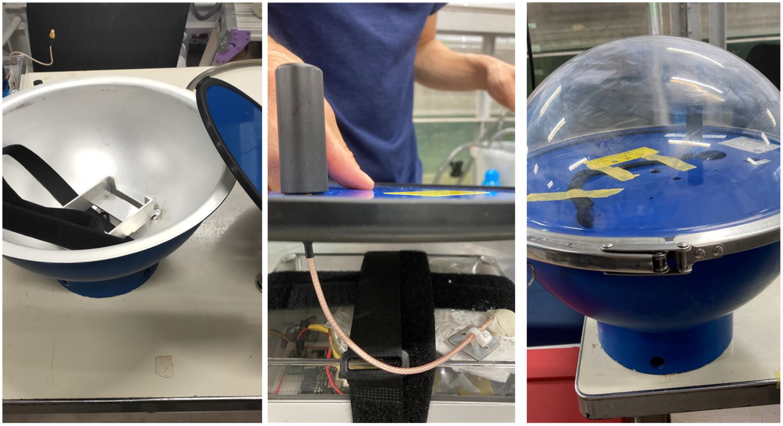
2.6. Total Cost and Assembly Process

The total bill of materials is presented in Table 2. We consider that around 0.5 h of work is needed to assemble a single instrument. No advanced electronics or hardware experience is required to build the instrument. At present, the assembly relies on a couple of soldering steps to connect the power supply module to the main board, and simply plugging the 9-dof sensor and the electronic switch controlling it into the main board using a couple of Qwiic I2C cables.
The total weight of the instrument depends on the size of the enclosure and the number of battery cells used. Typical weight is between 0.3 and 0.5 kg with 2 lithium D-cell batteries. The dimensions of the instrument are typically around 12 cm × 12 cm × 9 cm. Many of these parameters are part of design trade-offs. For example, more batteries increase weight and would make deployment from drones more challenging, but also allow to extend battery time. The use of a small enclosure allows for easier shipping and logistics and makes the instrument less likely to be discovered (and destroyed) by polar bears (in the Arctic), but means that even a relatively minor snowfall is enough to bury the instrument and interrupt GNSS and Iridium signals.
In addition to the construction costs, Iridium costs can be significant over time. Table 3 indicates the typical Iridium communication costs per month, for an instrument running with the default parameters (reducing the frequency of measurements will reduce costs accordingly).
Combining the building and the Iridium costs, the total cost per instrument, for an activity period of 6 months (which is reasonable for instruments deployed in the MIZ at the start of the ice formation season), is around 1200 USD, all included (noting that 4, rather than 2, LSH20 batteries will be necessary for such a deployment). Around 53% of this cost comes from the Iridium transmission fees; so, reducing the frequency of measurements when little activity of interest is happening will allow to significantly reduce the total cost of ownership.

3. Validation of the Instrument v2021

3.1. Autonomy and Satellite Communication Test in the Arctic: February 2021 Deployment

An early version of the instrument v2021, which performed drift tracking but no wave measurements, was deployed East of Svalbard in February 2021 [61]. This early version of the instrument was used to (i) validate the general design of the electronics; (ii) validate the low-power modes and the ability of the instrument to live for several months in the Arctic cold using just a couple of D-sized battery cells—in particular, regarding the power consumption of the iridium modem, which is hard to estimate; (iii) validate the satellite communication binary protocols.
This initial test was a success. The instrument was deployed on 24 February 2021, East of Svalbard. It then transmitted data for a few weeks, before a snow storm covered it with snow and blocked the iridium transmission. This loss of communications is a consequence of the design of the housing of the instrument, which relied on a box that was too weak to survive even just 10 cm of snow and will be addressed in future designs by using a box that is higher and does not get buried as easily. However, communication with the Iridium satellites was restored when the ice melted in late May 2021. Following this, the instrument freely floated in the open sea, traveling all the way from Svalbard to the close vicinity of Murmansk, and back and forth between Novaya Zemlya and Murmansk.
An overview of the trajectory is presented in Figure 3. At the time of writing this manuscript, i.e., January 2022, this instrument is still transmitting. The instrument was powered by 3 LSH20 batteries, which, since it measures only GNSS position each 30 min, should result in a battery life of around a bit over 1 year, following the data from Table 1. Therefore, this deployment validates the low-power design, and confirms that both the low-power sleep mode, the GNSS data acquisition, and the Iridium transmission (which have the power consumption that is most difficult to estimate) are correctly implemented and allow extended operation on battery alone.

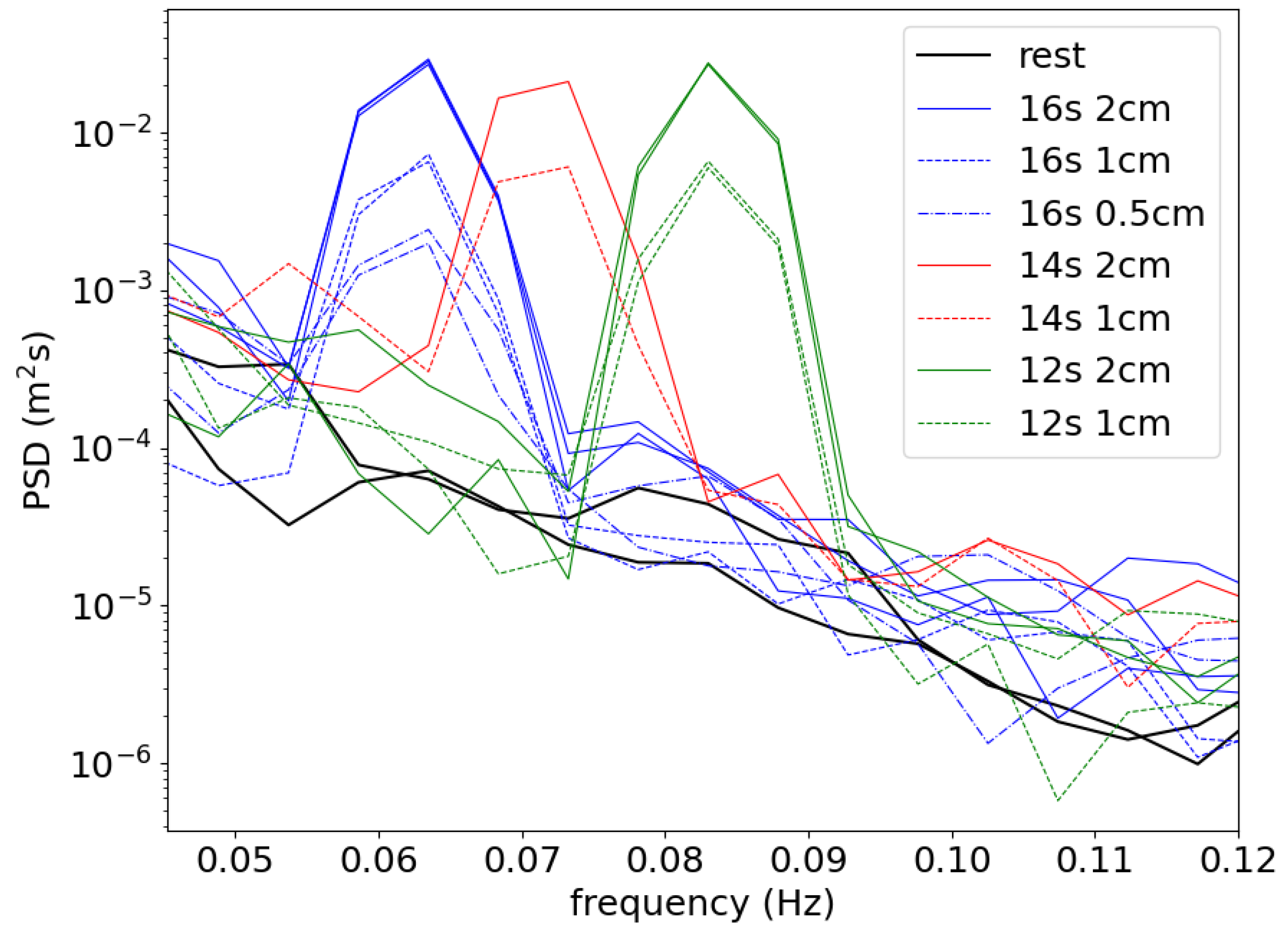
3.2. Experiments for Validation of Small-Amplitude, Low-Frequency Harmonic Vertical Displacement Measurements at the University of Tokyo’s Wave–Ice Tank Facility: July 2021 Laboratory Test

We conducted an experiment in July 2021 to evaluate the instrument v2021 accuracy for measuring small-amplitude harmonic vertical displacement representative of waves in ice. This experiment allows to fully validate (i) the acquisition of raw data from the 9-dof sensor, (ii) the processing algorithm and scaling factors used in the low-level signal processing code, and (iii) the data encoding used for transmitting the information back to the user. The experiment took place in the wave–ice tank facility at the Kashiwa campus of the University of Tokyo, Japan. In our case, however, the instrument v2021 prototype was placed on the top of the wavemaker paddle (which is a plundging wedge, vertical displacement paddle), rather than in the water (see Figure 4); so, it measured the vertical motion of the wavemaker itself, which is known to a very high accuracy thanks to the use of a closed-loop control. Indeed, even given the presence of a damping beach, it would be challenging in such a small wavetank to avoid reflections and standing waves, and to provide waves of sufficient amplitude at such low frequencies. By contrast, by placing the instrument on top of the paddle that is controlled by a closed-loop control system, we ensure that the vertical displacement of the instrument is exactly equal to the one specified in the control system. In this section, we will refer to the displacement prescribed as “wavemaker signal”, to emphasize that the signal we measure is the vertical displacement of the plunger-type wavemaker on which the instrument sits, rather than the motion of the water.
The experiment aims to evaluate the instrument accuracy when it measures centimeter-scale vertical displacement signals at low frequencies corresponding to typical waves in ice conditions. As such, we tested the instrument using both 1 and 2 cm amplitude sinusoidal wavemaker vertical motion for 12, 14, and 16 s periods (as well as an “extreme” test with 0.5 cm amplitude and 16 s period, to test the very limit of the instrument sensitivity), which resemble lower-bound wave signals that were previously measured in ice-covered ocean [14]. The spectral analysis setup was slightly modified from that of Section 2.2 so that each test case duration was reduced from 20 min to roughly 7 min in order to be able to perform the tests within the allocated time slot. For this, the segment overlap was reduced to 50% (corresponding to 1024 points), which yields a total number of 3 segments per 7 min measurement interval. All other processing configurations remained the same as Section 2.2.
The wavemaker signal experiment results are summarized in Table 4. The frequency of the wavemaker motion was not tuned to the exact frequency bins; nevertheless, the peak of the energy was consistently captured in the nearest frequency bin, as reflected in Table 4. Then, the best estimate of the wave amplitude can be derived as
A m o n o = d f × S ( i 1 ) 2 + S ( i ) 2 + S ( i + 1 ) 2 ,
where S ( i ) is the spectrum produced by the instrument, taken at the peak of the amplitude spectrum, and we consider also the neighboring frequency bins. The results of the wavemaker signal experiments summarized in Table 4 indicate that the instrument is capable of measuring monochromatic wave amplitudes of 1 to 2 cm with roughly 0.1 cm accuracy.
The spectra obtained during these tests, as well as two spectra corresponding to the instruments while at rest, are presented in Figure 5. As visible there, the noise background of the instrument increases slightly when motion is present, which may be explained by a variety of reasons (small vibrations in the wave paddle mechanism when it is undergoing displacement, diffusion of numerical noise in the processing algorithms, inherent properties of the 9-dof sensor). However, the increase in the noise threshold when there is motion remains very limited. The signal-to-noise ratio is superior or equal to a factor of 50 in all experiments, except for the smaller waves (0.5 cm at 16 s period), in which case the signal-to-noise ratio is around 10. This means that, even in this last “extreme” test case, the signal-to-noise ratio is still good enough to clearly distinguish the motion from the noise floor, though noise starts to be visible in the integrated statistics, as discussed in the previous paragraph and in Table 4.
Following this successful laboratory validation, we decided to perform a field validation experiment in the Arctic, which is described in the next subsection.

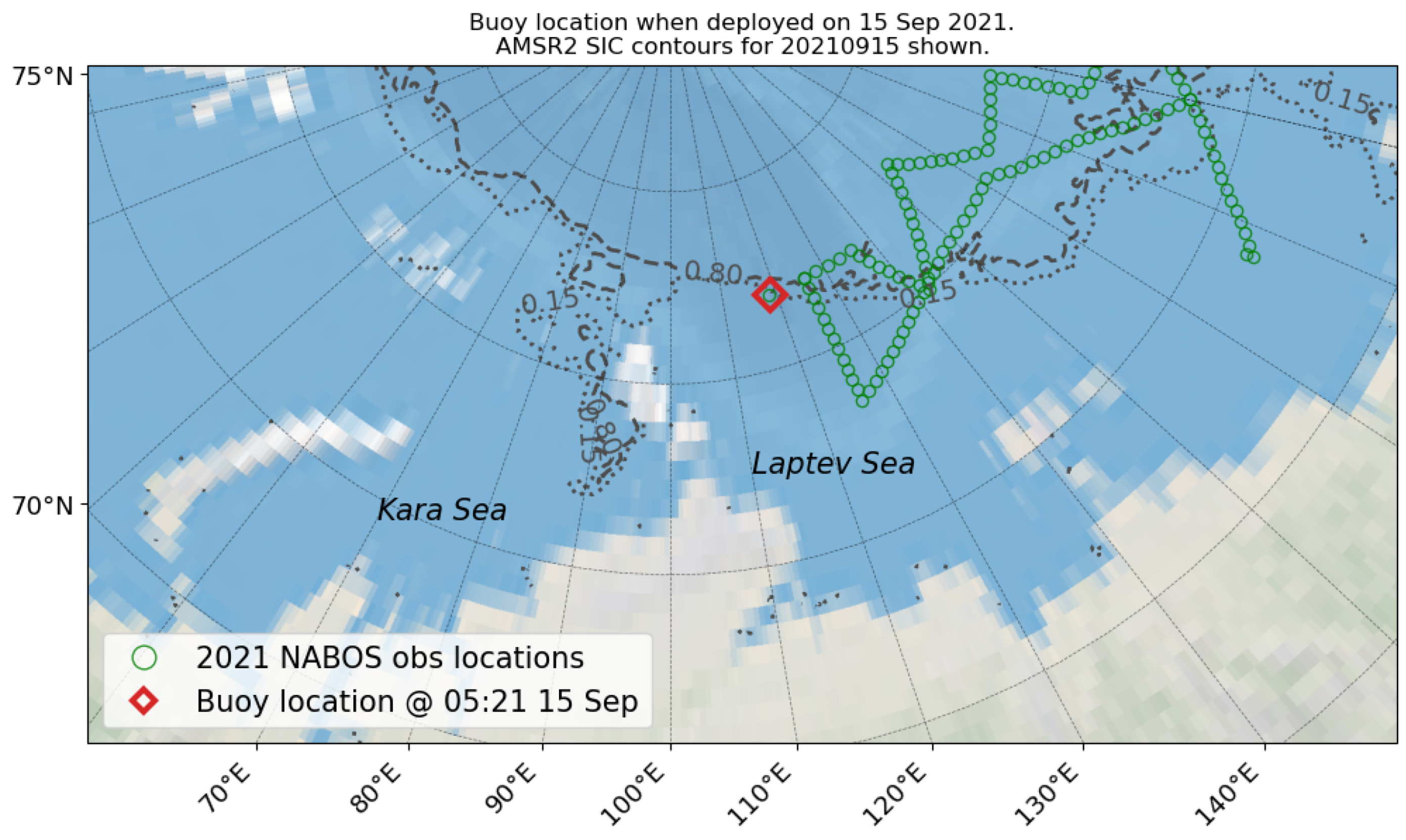
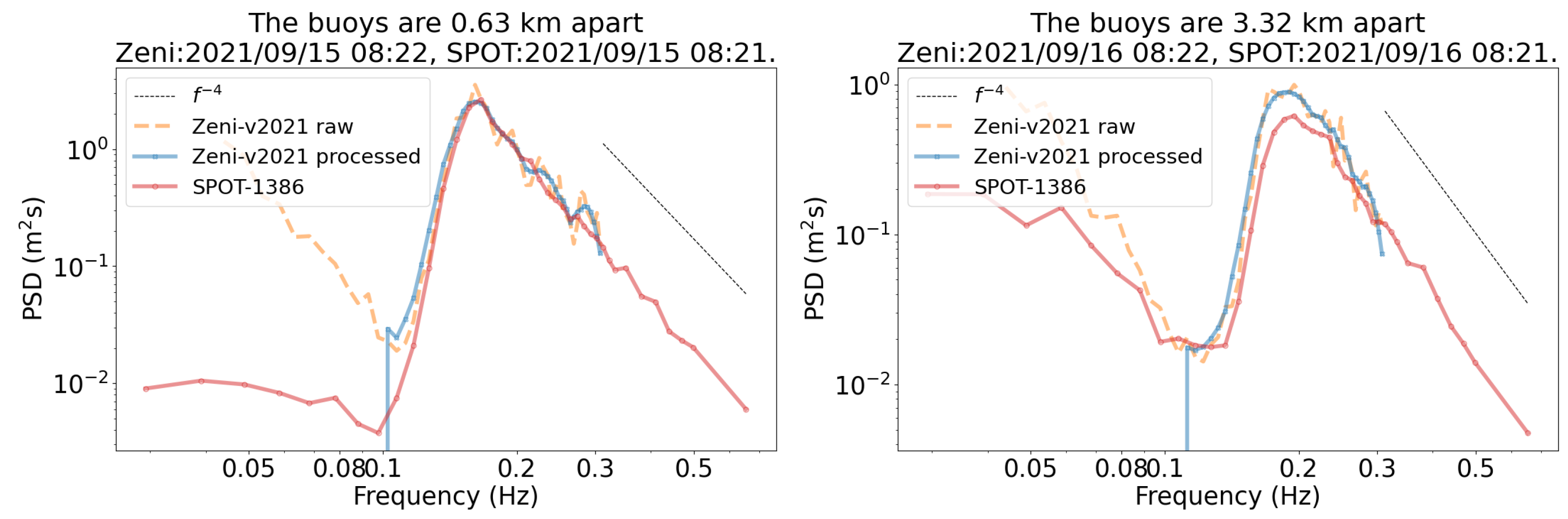
3.3. 2021 NABOS Expedition and Comparison with SOFAR Spotter Buoy in the Marginal Ice Zone in the Arctic: September 2021 Deployment

The first field deployment opportunity for the full-feature instrument v2021 was the 2021 Nansen and Amundsen Basins Observational System (NABOS) expedition (https://uaf-iarc.org/nabos-cruises/, accessed on 15 January 2022), which was performed in the context of the ArCS II Japan-Russia-Canada International Exchange Program (https://sites.google.com/edu.k.u-tokyo.ac.jp/arcsii-iep-jrc/main, accessed on 15 January 2022).
A v2021 instrument was assembled in a Zeni Lite drifting buoy, referred to as Zeni-v2021 in the following (see Appendix B for the buoy assembly details). This instrument was deployed alongside a commercial wave-measuring device (SOFAR Spotter drifting buoy, https://www.sofarocean.com/products/spotter, accessed on 15 January 2022), referred to as SPOT-1386 in the following. The key difference of the Spotter compared with the instrument v2021 is that the Spotter measures surface displacements based on GNSS signal.
On 15 September 2021, both buoys were deployed adjacent to the ice edge in the central Arctic Ocean (North of the Laptev Sea), at a location of 81.915 N 118.763 E, at around 05:05 UTC. The buoy deployment location is shown in Figure 6, which is overlaid with 0.15 and 0.80 sea ice concentration (SIC) contours based on the Advanced Microwave Scanning Radiometer 2 (AMSR2) data [62].
The two buoys drifted apart roughly 1 km within 8 h of being deployed and farther than 3 km after 24 h. Given that the ocean surface conditions near the ice edge are heterogeneous, we compared the instrument v2021 spectrum with that of SPOT-1386 following the deployment, when they were still close to each other. The buoy spectra compared generally well when the buoy distance was less than 1 km. The left panel in Figure 7 shows the buoy spectra at 08:21 15 September 2021, which corresponds to a moderate significant wave height H m 0 = 1.62 m. The comparison indicates that the spectra compare well when the low-frequency noise, which is typical in accelerometers, is discarded. Here, the method that was previously used in [63,64] was applied to remove this noise from Zeni-v2021 spectra. An ideal filter was applied to remove data below the lowest-frequency local minimum of the smoothed spectrum. In addition, another spectra comparison on 08:21 16 September is also provided on the right panel in Figure 7. By this time, the buoys were farther than 3 km apart, so there was a slight difference in energy levels between the two buoys but the general shape of the spectra is comparable. These buoy spectra comparisons indicate that the instrument v2021 can be used to measure ocean waves and is a full scale, fieldwork validation of the algorithms and processing used.
Spotter buoys, without solar radiation recharge at high latitude during the winter season, have only a short life span, and SPOT-1386 ran out of battery on 30 September 2021. Analysis into the colocated deployment in and near the Marginal Ice Zone MIZ is ongoing and will be presented in a separate, science-focused paper. Notwithstanding, a comparison of wave periods (peak period T p and spectral period T 0 m 1 ) when the buoys were less than 5 km-apart agree within better than 5%. In addition, the part of the dataset for which both instruments are frozen in the ice indicates that the noise level of the IMU-based instrument (typically around 0.1 cm) is much better than that of the Spotter buoy (typically around 1 cm), which is expected due to the different data sampling techniques used (GPS vs. 9-dof). This provides further support that Zeni-v2021 captured consistent energy densities to those of SPOT-1386 and that the Zeni-v2021 is actually better suited for measuring small waves in ice. Note that the analysis into the Zeni-v2021 and SPOT-1386 colocated deployment is described in a manuscript under preparation, which is why these data are not released in the present technical paper.
Regarding battery life, the estimated deployment duration for hourly wave sampling rate was 3.3 months based on Table 1, where two Tadiran D-cell batteries (TL-5930/S), each with 19 Ah capacity, were used as the power source. The instrument stopped transmitting, likely due to an empty battery, in mid-December, i.e., 3 months after the start of the deployment. This corresponds well with the estimated battery life and is an additional confirmation of the quality of the hardware and software design, in particular, regarding the implementation of low-power modes.

3.4. The “Floatenstein” Drifting Buoy in the Caribbeans: November 2021

A small-scale, home-produced drifting buoy was built following the v2021 design in the context of the OneOcean expedition, a circumnavigation by the Norwegian tall ship Statsraad Lehmkuh. The electronics are identical to everything that was discussed above, except for the battery solution used. Indeed, since the instrument had to be transported by plane in the checked luggage of an expedition member, two traditional alkaline D-cell batteries were used instead of the Li-batteries of the other instruments. A standard rectangular rigid plastic enclosure of size 12 cm × 12 cm × 9 cm was used as the main body of the buoy. Since alkaline batteries are heavier than lithium batteries, this resulted in too low buoyancy. As a consequence, we added small chunks of styrofoam (wrapped in duct tape to protect from abrasion from the elements) on the sides of the rigid plastic enclosure in order to increase buoyancy. These additional buoyancy elements were set in place using cable ties and glued in position using bathroom silicone sealant. In addition, the rigid plastic box was fully sealed with epoxy glue, to make it completely watertight. Finally, a keel composed of diverse scrap metallic parts (spare screws and bolts), packed in duct tape, was fixed at the bottom of the plastic enclosure to improve its static stability. This combination of disparate building materials gave a very peculiar appearance to the drifting buoy, which got nicknamed humorously as “Floatenstein” (Floating-Frankenstein). A picture of the instrument, fully built before being shipped, is presented in Figure 8.
Despite its unusual appearance, Floatenstein proved to be a robust and well-functioning drifter. Floatenstein was released in the open ocean on 11 November 2021, and, at the time of writing this manuscript (January 2022), Floatenstein has been active for little over two months and is working nominally. Data transmitted include (i) GPS position sampled each 30 min and (ii) vertical wave spectrum sampled each 2 h, similar to what is described in Section 2.
In order to validate the good functioning of Floatenstein and the electronics inside, we compare the wave data transmitted by Floatenstein with direct satellite altimeter measurements. The Wavy software package (see https://github.com/bohlinger/wavy, accessed on 15 January 2022, Bohlinger et al. [65]) is used to perform (i) gathering of relevant satellite data, (ii) collocation with the position of Floatenstein, and (iii) extraction of relevant fields. For the collocation process, the temporal and spatial constraints are 30 min and 50 km, respectively. Four satellite missions had coinciding satellite measurements: Sentinel-3A/B, Jason-3, and the altimeter mounted on CFOSAT. The satellite observations are of level 3 processing quality and are publicly available in the Copernicus CMEMS archive https://resources.marine.copernicus.eu/product-detail/WAVE_GLO_WAV_L3_SWH_NRT_OBSERVATIONS_014_001/INFORMATION, accessed on 15 January 2022.
Results of the comparison between Floatenstein and satellite data are presented in Figure 9. The satellite data are naturally spaced in time, due to the orbital pattern of the satellites collecting the data. The wave statistics reported by Floatenstein lies within the typical error margin of the direct observation by the satellites, which is visible as the spread in significant wave height over each small transect cutting the trajectory of Floatenstein. This is an additional confirmation of the good functioning of the electronics and firmware of the instrument v2021, as well as an illustration that even coarse drifters are able to accurately measure wave properties, as long as these are small enough to follow the motion of the waves. Indeed, the amplitude of the hydrodynamic response of the buoy itself is typically a fraction of the size of the buoy. This could, in theory, reach up to several tens of cm for large floating buoys with a typical size of several meters as is commonly found for the commercially available moored system, which has, historically, created a focus on developing wave buoys with a small hydrodynamic response. Our small buoy, by contrast, has a typical size of 10 cm, which implies that even a “bad” hydrodynamic response, leading to a displacement response in waves of several tens of percents of the buoy’s size, is still only a few centimeters in amplitude, well below typical stochastic noise and uncertainty of stochastic wave measurements in the open ocean. This is similar to other small buoys developed to measure specifically the high-frequency part of the wave spectrum [66].

4. Conclusions and Future Work

This work introduces a new design of waves in ice instrument. This instrument is able to perform measurements of sea ice drift using a GNSS module and to measure waves in ice up to a high degree of accuracy (the noise threshold corresponds to a significant wave height of around 0.1 cm for waves with period 16 s, as demonstrated in the laboratory experiments), using an inexpensive 9-degrees-of-freedom sensor and extensive signal processing and noise reduction techniques. In addition, this instrument costs only around slightly under 650 USD in electronics components (including taxes), raw materials, and assembly time, which is around 10 times less expensive to build than the closest, least-expensive commercial alternative we know about (the Sofar Spotter buoy), while being both more sensitive and much better adapted to working in the polar night, when solar input is not available. Battery autonomy using a couple of Lithium D-cells is around 4.5 months, and this can be easily increased by adding more cells if needed. Assembly time has been cut down to no more than typically half an hour per instrument when building a small series of these, thanks to the use of highly integrated open-source development boards, and requires no advanced electronics skills. The code is provided as open source together with the full design blueprints and assembly instructions. Binary precompiled firmware versions are provided for rapid upload to the electronics boards. Additional sensors can easily be added to the instruments. Two-way communications are implemented through highly optimized binary protocols and take place over Iridium, which enables global coverage. All data measurements take place at a fixed time thanks to the real-time clock available on board to allow easy time synchronization, and data are buffered on board the instrument to avoid data loss in case of temporary failure in establishing an iridium communication.
This set of characteristics is, as a whole, and to the best of our knowledge, unrivaled by any commercial or open-source instrument. These drastic improvements in cost and power efficiency, compared even with previous open-source instruments such as the one described in Rabault et al. [51], are made possible by the use of a cutting edge smartwatch processor, which can handle all of the logging and data processing workloads. This is, to the best of our knowledge, the fist time that such an instrument has been built without the need for an expensive, data-hungry, embedded microcomputer, and the first time the full logging, data processing, and communication workload is controlled from a single, power-efficient, low-cost microcontroller. In addition, this design is both modular and adapted to not only measurements of sea ice drift and waves in ice but also for open ocean measurements, as we have shown in the validation section.
We validated the design and signal processing code through a number of test campaigns in the laboratory, in the open water, and on sea ice. Results indicate agreement within typically 5% with state of the art reference instruments and measurement methods and confirm the robustness of the design as well as its power efficiency. In particular, the low power consumption of the instrument (which is always challenging to get right, as any error in the code or hardware design can easily increase the sleep power by a few milliamps, which, while it sounds little, drains battery over time) is confirmed during a deployment in the Arctic, and the accuracy of the wave measurements and wave data processing code are confirmed in several test cases.
This work, while purely technical, is in our opinion a groundbreaking step towards bringing open-source, inexpensive, easy to build, modular, power-efficient instrumentation to the field of in situ study of waves in ice in particular and oceanographic measurements in general. Indeed, our design has also proven to be highly efficient both as a traditional open ocean drifter and wave buoy. We expect that this design will significantly reduce the barrier to entry for new research groups to monitor waves in ice; sea ice drift patterns; and similarly, wave activity and ocean upper layer drift and currents in the open ocean; and be a possible platform for public outreach since the design is simple enough to be assembled for example by high school students. This design can also be used as a basic building block for setting up a variety of instruments—such as weather stations, environmental loggers, and wildlife monitoring instruments—by connecting specific sensors and adding extra modules to the firmware, while taking advantage of the power efficiency and iridium connectivity of the main electronics board.
Another key improvement brought by the present design is its very limited weight and size. Typically, our implementations of the design occupy a space of 12 cm × 12 cm × 9 cm and weight between 0.3 and 0.5 kg. This is small and light enough to be deployed, for example, from a medium size quadcopter drone or from a fishing rod several meters long. This could prove very important in practice when releasing large numbers of drifters in the Arctic and Antarctic, since (i) changing the course of an icebreaker and forcing it to make many (even short) stops to put instrumentation on the ice has a large footprint on the operation of the ship and a high cost, while (ii) flying a quadcopter drone to deploy instrumentation on the ice, or dropping instrumentation on-the-go while the boat is steaming using a long rod, would have zero marginal cost for an expedition.
As a final technical word, we want to say that, while we have released the instrument design, code, and validation data already since we believe that it may already be of value for other groups, there are a number of ongoing improvements that are taking place and will continue after this paper is published. First, we are working on adding the possibility to store large amounts of data using a two-step memory setup (i.e., a Ferromagnetic RAM for fast, low-power storage of data on the fly and a SD card for slow long-term archiving). This will make the instrument even more valuable in contexts where it can be recovered after deployment, since this will allow us to store and recover time series that are, at present, only stored temporarily in RAM for performing wave spectrum computation. Second, we will work in the future on adding full-directional wave spectrum information. Finally, when these additions are done, a major code rewrite, taking into account all the lessons learned while developing this instrument, will be performed to make the code even easier to extend, test, and reuse. When these further refinements are implemented, we will also consider designing an open-source printed circuit board, to lower even further the amount of work needed to assemble the electronics of the instrument. Ultimately, if there is interest from the community, we hope to provide an all-in-one, fully integrated, low-cost electronics boards that will be a true turn-key solution.

Author Contributions

Conceptualization, J.R., T.N., M.M., Ø.B., J.V., L.R.H., T.W., M.J. (Mark Johnson), G.S., M.J. (Malin Johansson), K.H.C., A.G., A.J., O.G., A.M. and A.B.; methodology, J.R. and T.N.; software, J.R., G.H. and P.B.; validation, J.R., T.N., M.M., Ø.B., J.V., L.R.H., P.B., T.K. (Tsubasa Kodaira) and T.K. (Tomotaka Katsuno); formal analysis, J.R., T.N. and P.B.; investigation, J.R., T.N., M.M. and L.R.H.; resources, M.M., Ø.B., L.R.H., T.W., M.J. (Mark Johnson), K.H.C. and A.B.; data curation, J.R., T.N. and P.B.; writing J.R.; visualization, J.R., T.N. and P.B.; funding acquisition, J.R., M.M., Ø.B., T.W., M.J. (Malin Johansson), K.H.C., A.J., A.M. and A.B. All authors have read and agreed to the published version of the manuscript.

Funding

This work was funded by the Research Council of Norway through ThinTEC (project number A321200), Norwegian Polar Institute through ThinIce (project number 66017); the ArCS II Japan-Russia-Canada International Exchange Program; the Arctic Challenge for Sustainability II Project (ArCS II Project, Program Grant Number JPMXD1420318865); the JSPS KAKENHI Grant Number JP 19H00801, 19H05512, and 21K14357; the DOFI Petromaks II project (funding to the University of Oslo, by the Research Council of Norway funding, grant number 28062).

Institutional Review Board Statement

Not applicable.

Informed Consent Statement

Not applicable.

Data Availability Statement

Available by request to the corresponding author.

Acknowledgments

We want to thank Frank Nilsen and Ilker Fer for inviting us to join the Nansen Legacy Cruise PC-2: Winter Process Cruise, during which we tested the first early prototypes of the v2021. Our warmest thanks go to all the participants of this cruise and to the crew of the R/V Kronprins Haakon for their help during this cruise and the very friendly weeks spent together onboard the ship. Our warmest thanks go to Ceslav Czyz, Zoe Koenig, and Helge Bryhni for many interesting discussions about the development of custom-made software and hardware for geoscience measurements. We also want to thank the Norwegian Meteorological Institute for continuous support of our efforts towards building an open-source instrumentation community and for support of our open-source release policy. This work was supported partly through several projects; in particular, ThinTEC (project number A321200) and ThinIce (project number 66017), funded by the Research Council of Norway and the Norwegian Polar Institute. Participation to the Nansen Legacy PC-2 cruise and instrumentation used there, as well as part of the data analysis, were funded through the Nansen Legacy project (NFR-276730) and FOCUS project (NFR-301450). In addition, some synergies with the Machine Ocean project funded by the research Council of Norway (project number 303411) helped in the present developments. We gratefully acknowledge support from the Japan Agency for Marine-Earth Science and Technology, in particular, for constructing the ice-wave tank at the Univ. of Tokyo. The 2021 NABOS buoy deployment was supported by the ArCS II Japan-Russia-Canada International Exchange Program (https://sites.google.com/edu.k.u-tokyo.ac.jp/arcsii-iep-jrc/main, accessed on 5 January 2022). TW is grateful to Tatiana Alekseeva of the Russian Arctic and Antarctic Research Institute for making our NABOS deployment possible. TN, TW, TKo, and TKa are grateful to Profs Kanna and Tateyama for deploying our wave buoys during 2021 NABOS expedition. Some of this work was performed in the context of the Arctic Challenge for Sustainability II Project (ArCS II Project, Program Grant Number JPMXD1420318865). A part of this study was also conducted under JSPS KAKENHI Grant Numbers JP 19H00801, 19H05512, and 21K14357. This study was supported partly by the Grant for Joint Research Program of the Japan Arctic Research Network Center. We also want to thank the One Ocean expedition and the University of Bergen course SDG313 for facilitating deployment of the Floatenstein drifter in the Caribbean. This work was also partially conducted in the context of the DOFI Petromaks II project (funding to the University of Oslo, by the Research Council of Norway, grant number 28062). We want to thank Jim Thomson, as well as the members of his group, for the very interesting and stimulating discussions about open-source instrumentation and measurements of ocean waves using open-source electronics. Finally, we want to acknowledge and thank the Arduino community and ecosystem as well as Sparkfun and the community around it for making high-performance microelectronics easily available to nonexperts. Our development of open-source instrumentation as is presented in this work would not be possible without the amazing work and tools offered by these communities.

Conflicts of Interest

The authors declare no conflict of interest.

Correction Statement

This article has been republished with a minor correction to an author's ORCID. This change does not affect the scientific content of the article.

Appendix A. Open-Source Release and Founding of an Open-Source Community

All the code, instructions, and postprocessing scripts necessary to build, program, and use the instrument v2021 are available as open-source hardware and software on Github under a MIT license at the following URL: https://github.com/jerabaul29/OpenMetBuoy-v2021a, accessed on 5 January 2022.

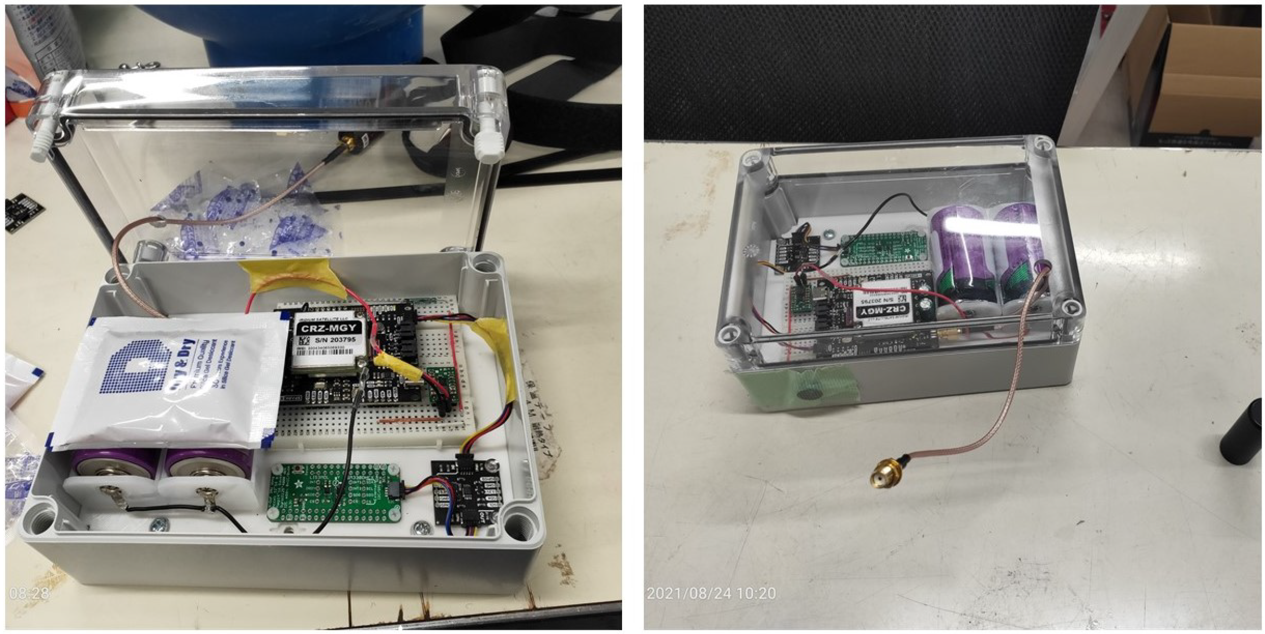
Appendix B. Zeni-v2021 Assembly for the 2021 NABOS Cruise

The Artemis Global Tracker and other electronics components listed in Section 2.1 were enclosed in a water-resistant Takachi box as shown in Figure A1. Deployment in the open water requires a floating enclosure that is durable and watertight. For our purpose, we used a commercial Zeni Lite drifting buoy (https://www.zenilite.co.jp/prod/new-chikuden.html, accessed on 5 January 2022), which was purchased by the University of Tokyo several years ago as a floating enclosure. Images of the floating enclosure setup are shown in Figure A2. The Zeni Lite drifting buoy has open space inside where the Takachi box was fixed. This space is easily accessible and also high enough for the antenna to be fixed on the upper half of the buoy. The water tightness is achieved via an O-ring placed underneath the blue plate. When the steel brace is fastened, pressure is evenly applied around the buoy housing where the top and bottom parts of the buoy are joined. The instrument v2021 deployed in the Arctic Ocean as described in Section 3.3, is referred to as Zeni-v2021 in the main text, because the instrument v2021 was assembled in the Zeni Lite drifting buoy enclosure.
Figure A1. Illustrations of the instrument v2021 electronics components enclosed in a water-resistant Takachi box.
Geosciences 12 00110 g0a1
Figure A2. Illustrations of Zeni Lite drifting buoy being used as a floating housing. The left image shows the bottom part of the buoy where the Takachi box was fixed. The middle image shows how the antenna was attached through the blue plate. The right image shows the assembled Zeni-v2021.
Geosciences 12 00110 g0a2

References

  1. Squire, V.A. Ocean wave interactions with sea ice: A reappraisal. Annu. Rev. Fluid Mech. 2020, 52, 37–60. [Google Scholar] [CrossRef]
  2. Smith, F.; Korobkin, A.; Parau, E.; Feltham, D.; Squire, V. Modelling of sea-ice phenomena. Philos. Trans. R. Soc. Math. Phys. Eng. Sci. 2018, 376, 20180157. [Google Scholar] [CrossRef]
  3. Zhao, X.; Shen, H.H. Three-layer viscoelastic model with eddy viscosity effect for flexural-gravity wave propagation through ice cover. Ocean. Model. 2018, 131, 15–23. [Google Scholar] [CrossRef]
  4. Golden, K.M.; Bennetts, L.G.; Cherkaev, E.; Eisenman, I.; Feltham, D.; Horvat, C.; Hunke, E.; Jones, C.; Perovich, D.K.; Ponte-Castaneda, P.; et al. Modeling sea ice. Not. Am. Math. Soc. 2020, 67, 1535–1555. [Google Scholar] [CrossRef]
  5. Roach, L.A.; Bitz, C.M.; Horvat, C.; Dean, S.M. Advances in modeling interactions between sea ice and ocean surface waves. J. Adv. Model. Earth Syst. 2019, 11, 4167–4181. [Google Scholar] [CrossRef]
  6. Sutherland, G.; Rabault, J.; Christensen, K.H.; Jensen, A. A two layer model for wave dissipation in sea ice. Appl. Ocean. Res. 2019, 88, 111–118. [Google Scholar] [CrossRef]
  7. Williams, T.D.; Rampal, P.; Bouillon, S. Wave–ice interactions in the neXtSIM sea-ice model. Cryosphere 2017, 11, 2117–2135. [Google Scholar] [CrossRef]
  8. Sree, D.K.; Law, A.W.K.; Shen, H.H. An experimental study of gravity waves through segmented floating viscoelastic covers. Appl. Ocean. Res. 2020, 101, 102233. [Google Scholar] [CrossRef]
  9. Rabault, J.; Sutherland, G.; Jensen, A.; Christensen, K.H.; Marchenko, A. Experiments on wave propagation in grease ice: Combined wave gauges and particle image velocimetry measurements. J. Fluid Mech. 2019, 864, 876–898. [Google Scholar] [CrossRef]
  10. Li, H.; Gedikli, E.D.; Lubbad, R. Laboratory study of wave-induced flexural motion of ice floes. Cold Reg. Sci. Technol. 2021, 182, 103208. [Google Scholar] [CrossRef]
  11. Sutherland, G.; Halsne, T.; Rabault, J.; Jensen, A. The attenuation of monochromatic surface waves due to the presence of an inextensible cover. Wave Motion 2017, 68, 88–96. [Google Scholar] [CrossRef]
  12. Marchenko, A.; Haase, A.; Jensen, A.; Lishman, B.; Rabault, J.; Evers, K.U.; Shortt, M.; Thiel, T. Laboratory Investigations of the Bending Rheology of Floating Saline Ice and Physical Mechanisms of Wave Damping In the HSVA Hamburg Ship Model Basin Ice Tank. Water 2021, 13, 1080. [Google Scholar] [CrossRef]
  13. Kohout, A.L.; Smith, M.; Roach, L.A.; Williams, G.; Montiel, F.; Williams, M.J.M. Observations of exponential wave attenuation in Antarctic sea ice during the PIPERS campaign. Ann. Glaciol. 2020, 61, 196–209. [Google Scholar] [CrossRef]
  14. Voermans, J.J.; Rabault, J.; Filchuk, K.; Ryzhov, I.; Heil, P.; Marchenko, A.; Collins, C.O., III; Dabboor, M.; Sutherland, G.; Babanin, A.V. Experimental evidence for a universal threshold characterizing wave-induced sea ice break-up. Cryosphere 2020, 14, 4265–4278. [Google Scholar] [CrossRef]
  15. Løken, T.K.; Rabault, J.; Jensen, A.; Sutherland, G.; Christensen, K.H.; Müller, M. Wave measurements from ship mounted sensors in the Arctic marginal ice zone. Cold Reg. Sci. Technol. 2021, 182, 103207. [Google Scholar] [CrossRef]
  16. Thomson, J.; Fan, Y.; Stammerjohn, S.; Stopa, J.; Rogers, W.E.; Girard-Ardhuin, F.; Ardhuin, F.; Shen, H.; Perrie, W.; Shen, H.; et al. Emerging trends in the sea state of the Beaufort and Chukchi seas. Ocean Model. 2016, 105, 1–12. [Google Scholar] [CrossRef]
  17. Løken, T.K.; Marchenko, A.; Ellevold, T.J.; Rabault, J.; Jensen, A. An investigation into the turbulence induced by moving ice floes. arXiv 2021, arXiv:2104.02378. [Google Scholar]
  18. Løken, T.K.; Ellevold, T.J.; de la Torre, R.G.R.; Rabault, J.; Jensen, A. Bringing optical fluid motion analysis to the field: A methodology using an open source ROV as a camera system and rising bubbles as tracers. Meas. Sci. Technol. 2021, 32, 095302. [Google Scholar] [CrossRef]
  19. Voermans, J.J.; Liu, Q.; Marchenko, A.; Rabault, J.; Filchuk, K.; Ryzhov, I.; Heil, P.; Waseda, T.; Nose, T.; Kodaira, T.; et al. Wave dispersion and dissipation in landfast ice: Comparison of observations against models. Cryosphere 2021, 2021, 1–26. [Google Scholar] [CrossRef]
  20. Sutherland, G.; Rabault, J. Observations of wave dispersion and attenuation in landfast ice. J. Geophys. Res. Ocean. 2016, 121, 1984–1997. [Google Scholar] [CrossRef]
  21. Rabault, J.; Sutherland, G.; Gundersen, O.; Jensen, A. Measurements of wave damping by a grease ice slick in Svalbard using off-the-shelf sensors and open-source electronics. J. Glaciol. 2017, 63, 372–381. [Google Scholar] [CrossRef]
  22. Marchenko, A.; Rabault, J.; Sutherland, G.; Collins, C.O.; Wadhams, P.; Chumakov, M. Field observations and preliminary investigations of a wave event in solid drift ice in the Barents Sea. In Proceedings of the International Conference on Port and Ocean Engineering under Arctic Conditions, Port and Ocean Engineering under Arctic Conditions, Busan, Korea, 11–16 June 2017. [Google Scholar]
  23. Marchenko, A.; Wadhams, P.; Collins, C.; Rabault, J.; Chumakov, M. Wave-ice interaction in the north-west barents sea. Appl. Ocean. Res. 2019, 90, 101861. [Google Scholar] [CrossRef]
  24. Johnson, M.A.; Marchenko, A.V.; Dammann, D.O.; Mahoney, A.R. Observing Wind-Forced Flexural-Gravity Waves in the Beaufort Sea and Their Relationship to Sea Ice Mechanics. J. Mar. Sci. Eng. 2021, 9, 471. [Google Scholar] [CrossRef]
  25. Herman, A.; Evers, K.U.; Reimer, N. Floe-size distributions in laboratory ice broken by waves. Cryosphere 2018, 12, 685–699. [Google Scholar] [CrossRef]
  26. Horvat, C.; Tziperman, E. The evolution of scaling laws in the sea ice floe size distribution. J. Geophys. Res. Ocean. 2017, 122, 7630–7650. [Google Scholar] [CrossRef]
  27. Herman, A. Sea-ice floe-size distribution in the context of spontaneous scaling emergence in stochastic systems. Phys. Rev. E 2010, 81, 066123. [Google Scholar] [CrossRef]
  28. Herman, A. Spectral wave energy dissipation due to under-ice turbulence. J. Phys. Oceanogr. 2021, 51, 1177–1186. [Google Scholar] [CrossRef]
  29. Voermans, J.; Babanin, A.; Thomson, J.; Smith, M.; Shen, H. Wave attenuation by sea ice turbulence. Geophys. Res. Lett. 2019, 46, 6796–6803. [Google Scholar] [CrossRef]
  30. Smith, M.; Thomson, J. Pancake sea ice kinematics and dynamics using shipboard stereo video. Ann. Glaciol. 2020, 61, 1–11. [Google Scholar] [CrossRef]
  31. Herman, A. Wave-Induced Surge Motion and Collisions of Sea Ice Floes: Finite-Floe-Size Effects. J. Geophys. Res. Ocean. 2018, 123, 7472–7494. [Google Scholar] [CrossRef]
  32. Herman, A.; Wenta, M.; Cheng, S. Sizes and shapes of sea ice floes broken by waves—A case study from the East Antarctic coast. Front. Earth Sci. 2021, 9, 390. [Google Scholar] [CrossRef]
  33. Li, J.; Babanin, A.V.; Liu, Q.; Voermans, J.J.; Heil, P.; Tang, Y. Effects of Wave-Induced Sea Ice Break-Up and Mixing in a High-Resolution Coupled Ice-Ocean Model. J. Mar. Sci. Eng. 2021, 9, 365. [Google Scholar] [CrossRef]
  34. Ardhuin, F.; Otero, M.; Merrifield, S.; Grouazel, A.; Terrill, E. Ice breakup controls dissipation of wind waves across Southern Ocean sea ice. Geophys. Res. Lett. 2020, 47, e2020GL087699. [Google Scholar] [CrossRef]
  35. Herman, A. Wave-induced stress and breaking of sea ice in a coupled hydrodynamic discrete-element wave–ice model. Cryosphere 2017, 11, 2711–2725. [Google Scholar] [CrossRef]
  36. Roach, L.A.; Horvat, C.; Dean, S.M.; Bitz, C.M. An emergent sea ice floe size distribution in a global coupled ocean-sea ice model. J. Geophys. Res. Ocean. 2018, 123, 4322–4337. [Google Scholar] [CrossRef]
  37. Horvat, C.; Tziperman, E. A prognostic model of the sea-ice floe size and thickness distribution. Cryosphere 2015, 9, 2119–2134. [Google Scholar] [CrossRef]
  38. Mosig, J.E.M.; Montiel, F.; Squire, V.A. Comparison of viscoelastic-type models for ocean wave attenuation in ice-covered seas. J. Geophys. Res. Ocean. 2015, 120, 6072–6090. [Google Scholar] [CrossRef]
  39. Cheng, S.; Rogers, W.E.; Thomson, J.; Smith, M.; Doble, M.J.; Wadhams, P.; Kohout, A.L.; Lund, B.; Persson, O.P.; Collins, C.O., III; et al. Calibrating a Viscoelastic Sea Ice Model for Wave Propagation in the Arctic Fall Marginal Ice Zone. J. Geophys. Res. Ocean. 2017, 122, 8770–8793. [Google Scholar] [CrossRef]
  40. Kohout, A.L.; Penrose, B.; Penrose, S.; Williams, M.J. A device for measuring wave-induced motion of ice floes in the Antarctic marginal ice zone. Ann. Glaciol. 2015, 56, 415–424. [Google Scholar] [CrossRef]
  41. Rabault, J.; Sutherland, G.; Ward, B.; Christensen, K.H.; Halsne, T.; Jensen, A. Measurements of waves in landfast ice using inertial motion units. IEEE Trans. Geosci. Remote Sens. 2016, 54, 6399–6408. [Google Scholar] [CrossRef]
  42. Thomson, J.; Gemmrich, J.; Rogers, W.E.; Collins, C.O.; Ardhuin, F. Wave Groups Observed in Pancake Sea Ice. J. Geophys. Res. Ocean. 2019, 124, 7400–7411. [Google Scholar] [CrossRef]
  43. Kodaira, T.; Waseda, T.; Nose, T.; Sato, K.; Inoue, J.; Voermans, J.; Babanin, A. Observation of on-ice wind waves under grease ice in the western Arctic Ocean. Polar Sci. 2021, 27, 100567, Arctic Challenge for Sustainability Project (ArCS). [Google Scholar] [CrossRef]
  44. Ardhuin, F.; Stopa, J.; Chapron, B.; Collard, F.; Smith, M.; Thomson, J.; Doble, M.; Blomquist, B.; Persson, O.; Collins, C.O.; et al. Measuring ocean waves in sea ice using SAR imagery: A quasi-deterministic approach evaluated with Sentinel-1 and in situ data. Remote Sens. Environ. 2017, 189, 211–222. [Google Scholar] [CrossRef]
  45. Horvat, C.; Blanchard-Wrigglesworth, E.; Petty, A. Observing waves in sea ice with ICESat-2. Geophys. Res. Lett. 2020, 47, e2020GL087629. [Google Scholar] [CrossRef]
  46. Smit, P.; Houghton, I.; Jordanova, K.; Portwood, T.; Shapiro, E.; Clark, D.; Sosa, M.; Janssen, T. Assimilation of significant wave height from distributed ocean wave sensors. Ocean Model. 2021, 159, 101738. [Google Scholar] [CrossRef]
  47. Doble, M.; Mercer, D.J.; Meldrum, D.; Peppe, O.C. Wave measurements on sea ice: Developments in instrumentation. Ann. Glaciol. 2006, 44, 108–112. [Google Scholar] [CrossRef]
  48. Datawell Corporation. History of Datawell; Datawell Corporation: Haarlem, The Netherlands, 2001. [Google Scholar]
  49. Raghukumar, K.; Chang, G.; Spada, F.; Jannsen, T. Directional Spectrum Measurements by the Spotter: A New Developed Wave Buoy; University of New Orleans: New Orleans, LA, USA, 2019. [Google Scholar]
  50. Wilkinson, J.; Wadke, P.; Meldrum, D.; Mercer, D.; Doble, M.; Wadhams, P. The autonomous measurement of waves propagating across the Arctic Ocean. In Proceedings of the OCEANS 2007, Vancouver, BC, Canada, 29 September–4 October 2007; IEEE: Piscataway, NJ, USA, 2007; pp. 1–7. [Google Scholar]
  51. Rabault, J.; Sutherland, G.; Gundersen, O.; Jensen, A.; Marchenko, A.; Breivik, Ø. An open source, versatile, affordable waves in ice instrument for scientific measurements in the Polar Regions. Cold Reg. Sci. Technol. 2020, 170, 102955. [Google Scholar] [CrossRef]
  52. Sutherland, G.; Aguiar, V.; Hole, L.R.; Rabault, J.; Dabboor, M.; Breivik, Ø. Determining an optimal transport velocity in the marginal ice zone using operational ice-ocean prediction systems. Cryosphere Discuss 2021. [Google Scholar] [CrossRef]
  53. Thomson, J. Wave breaking dissipation observed with “SWIFT” drifters. J. Atmos. Ocean. Technol. 2012, 29, 1866–1882. [Google Scholar] [CrossRef]
  54. Keating, D. Fetch-Limited Wave Growth in Nootka Sound. Senior Thesis, University of Washington, School of Oceanography, Seattle, WA, USA, 2016. [Google Scholar]
  55. Thomson, J.; Moulton, M.; de Klerk, A.; Talbert, J.; Guerra, M.; Kastner, S.; Smith, M.; Schwendeman, M.; Zippel, S.; Nylund, S. A new version of the SWIFT platform for waves, currents, and turbulence in the ocean surface layer. In Proceedings of the 2019 IEEE/OES Twelfth Current, Waves and Turbulence Measurement (CWTM), San Diego, CA, USA, 10–13 March 2019; IEEE: Piscataway, NJ, USA, 2019; pp. 1–7. [Google Scholar]
  56. Defense Advanced Research Projects Agency. Ocean of Things; Defense Advanced Research Projects Agency: Arlington, VA, USA, 2021. [Google Scholar]
  57. Ambiq Inc. Ambiq Apollo3 BLU Microcontroller; Ambiq Inc.: Austin, TX, USA, 2021. [Google Scholar]
  58. Sparkfun Inc. Artemis Global Tracker; Sparkfun Inc.: Niwot, CO, USA, 2021. [Google Scholar]
  59. Pololu Inc. Pololu 3.3V Step-Up/Step-Down Voltage Regulator S7V8F3; Pololu Inc.: Las Vegas, NV, USA, 2021. [Google Scholar]
  60. Mouser Inc. MDRR-DT-15-25-F Reed Switch; Mouser Inc.: Mansfield, TX, USA, 2021. [Google Scholar]
  61. Nilsen, F.; Fer, I.; Baumann, T.M.; Breivik, Ø.; Czyz, C.; Frank, L.; Kalhagen, K.; Koenig, Z.; Kolås, E.H.; Kral, S.T.; et al. PC-2 Winter Process Cruise (WPC): Cruise Report; The Nansen Legacy Report Series; Septentrio Academic Publishing: Tromsø, Norway, 2021. [Google Scholar]
  62. Hori, M.; Yabuki, H.; Sugimura, T.; Terui, T. AMSR2 Level 3 Product of Daily Polar Brightness Temperatures and Product, 1.00. 2012. Available online: https://ads.nipr.ac.jp/data/meta/A20170123-003 (accessed on 23 July 2019).
  63. Waseda, T.; Webb, A.; Sato, K.; Inoue, J. Arctic Wave Observation by Drifting Type Wave Buoys in 2016. In Proceedings of the 27th International Ocean and Polar Engineering Conference, San Francisco, CA, USA, 25–30 June 2017; International Society of Offshore and Polar Engineers: Mountain View, CA, USA, 2017. [Google Scholar]
  64. Nose, T.; Webb, A.; Waseda, T.; Inoue, J.; Sato, K. Predictability of storm wave heights in the ice-free Beaufort Sea. Ocean Dyn. 2018, 68, 1383–1402. [Google Scholar] [CrossRef]
  65. Bohlinger, P.; Breivik, Ø.; Economou, T.; Müller, M. A novel approach to computing super observations for probabilistic wave model validation. Ocean Model. 2019, 139, 101404. [Google Scholar] [CrossRef]
  66. Yurovsky, Y.Y.; Dulov, V.A. MEMS-based wave buoy: Towards short wind-wave sensing. Ocean Eng. 2020, 217, 108043. [Google Scholar] [CrossRef]
Figure 1. Overview of waves in ice instruments, distinguishing between (i) commercial instruments, (ii) closed-source instruments, (iii) open source. Commercial instruments have been available for a long time, in particular the Datawell Waverider series of instruments (1), which goes back all the way to the 1960s [48]. More recently, the Sofar Spotter (2) has become a viable, lower-cost alternative, though there are a number of limitations, particularly regarding battery autonomy [49] and the price. A number of groups have developed satellite-connected autonomous instruments that have been described in research articles, but that remained closed source. A few instruments we know about were released in 2006 (3) [47,50], 2016 (4) [40], and 2021 (5) [24]. By contrast, our group has decided to release our designs as open source, so that they can be freely used and improved by other groups, starting in 2018 (6) [51] and now with the present design (7).
Geosciences 12 00110 g001
Figure 2. Full lineage of our present open-source instrument. Developing reliable autonomous instruments is a long-term effort. The development of our instrument can be tracked back to 2015 [41] and 2016 [21], though the instruments used at the time were simple loggers. Using loggers is still an attractive solution when the instruments can be recovered, and the logger v2016 design is still in use today. By contrast, our first truly autonomous, satellite-enabled instrument was designed in 2017–2018 [51], and the present instrument is the second iteration around this design.
Geosciences 12 00110 g002
Figure 3. Overview of the drift trajectory of the early prototype instrument deployed in February 2021, East of Svalbard. The interruption in the trajectory is due to a layer of snow covering the instrument that prevented satellite communications during a couple of months. The instrument then drifted freely in the open ocean. This validates the low-power design and confirms that the chosen design is able to sustain operations for several months using just a few D-cell Lithium batteries.
Geosciences 12 00110 g003
Figure 4. Illustration of the wavemaker experiment setup in the wave–ice tank of JAMSTEC (Japan Agency for Marine-Earth Science and Technology) at the Kashiwa campus of the University of Tokyo, Japan. The instrument v2021 location is shown by the yellow arrow.
Geosciences 12 00110 g004
Figure 5. Spectra obtained when testing the instrument v2021 in the laboratory. The signal-to-noise ratio is superior or equal to 50 for all test cases, except the “extreme” test case with displacements of amplitude 0.5 cm and period 16 s, where the signal-to-noise ratio is around 10. The noise threshold obtained when the instrument is at rest is actually slightly better than what was obtained with the instrument v2018 (compare the present plot with Figure 3 of Rabault et al. [51], curves “IMU 1” and “IMU 2”).
Geosciences 12 00110 g005
Figure 6. Zeni-v2021 and SPOT-1386 deployment location on 15 September 2021. The 2021 NABOS observation locations also shown in green markers and AMSR2-derived 0.15 and 0.80 Sea Ice Concentration (SIC) contours for the same day are overlaid.
Geosciences 12 00110 g006
Figure 7. Comparison of Zeni-v2021 and SPOT-1386 spectra at 08:21 15 September 2021 (left) and 08:21 16 September 2021 (right): the distances between the buoys were roughly 1 km and 3 km, respectively. Low-frequency noise of Zeni-v2021 spectra was removed by applying an ideal filter at the lowest frequency local minimum of the smoothed spectrum, similar to what was reported in Waseda et al. [63], Nose et al. [64], which is a common postprocessing step when working with accelerometer-derived wave data. This indicates agreement within typically 5% between the Sofar Spotter and the instrument v2021 measurements in the open water, before the instruments drift away from each other.
Geosciences 12 00110 g007
Figure 8. The “Floatenstein” drifting buoy. The main body of the buoy is a rectangular plastic box of dimensions 12 cm × 12 cm × 9 cm. Due to the use of alkaline batteries instead of lithium batteries, additional flotation elements were needed. These are the two rectangular elements on the side of the main body of the buoy, which are built from styrofoam chunks, wrapped in duct tape, and held in place by cable ties. The full box is sealed with epoxy to be perfectly watertight. To avoid the need for making holes in the box, the Iridium antenna is also taped in place inside the box, immediately under the lid, pointing 45 degrees upwards. The small cubic magnet (wrapped in duct tape to hold it in position under transport), which controls the magnetic switch glued on the inside of the box, is visible on the front panel of the main body of the drifter.
Geosciences 12 00110 g008
Figure 9. (Top): drift pattern of Floatenstein (colored continuous black line) and satellite measurement transects (colored points) over which wave characteristics are measured by the satellites. (Bottom): comparison of the Significant Wave Height (SWH) (i) reported by Floatenstein (continuous black line) and (ii) from satellite measurements on the corresponding measurement transects.
Geosciences 12 00110 g009
Table 1. Overview of the power consumption and resulting battery autonomy resulting from the different components of the instrument when using two nonrechargeable D-sized Lithium batteries. ‘Activity mode’ indicates the part of the workflow of the instrument that is being considered. ‘Activation frequency’ indicates a typical activation duration and frequency (though this is only indicative and may be modified either by using different parameters when programming the instrument, and/or by sending updated activity rates through the bidirectional iridium communication). ‘Current (mA)’ is the average current used in the corresponding mode when it is active. ‘mWh use per hour’ indicates the corresponding energy use for the given activation mode, following the formula mWh   Use   Per   Hour = Current ( mA ) × 3.3 ( V ) × ActivationFraction .
Activity ModeActivation FrequencyCurrent (mA)mWh Use per HourTime to Empty 2 Li D-Cells
sleepwhen not active0.31.07.3 years
gnss measurement2 min twice per hour303.32.2 years
wave measurement20 min every 2 h84.41.6 years
iridium transmission1 message per hourburst 250 mA100.7 years
typical use 18.70.39 years ≈ 4.6 months
Table 2. A representative list of components needed to build an instrument monitoring drift (GNSS) and wave activity (9-dof sensor). The assembly time for a single instrument, when assembling a series of 10 instruments in bulk, is about 0.5 h once the user is familiar with the design.
ComponentFunctionPrice (USD)Assembly Steps
Artemis Global Trackermain board, MCU, GNSS, Iridium375ready to use
GNSS + Iridium antennapassive antenna65screw on SMA cable
SMA extension cable 25 cmextension cable for antenna5screw on tracker
Qwiic power switchpower on and off 9-dof7disable LED, connect 9-dof and tracker
ISM330DHCX + LIS3MDL9-dof sensor18connect to power switch
Qwiic cables (x2)connect tracker, 9-dof, switch3connect power switch and 9-dof
3.3V Regulator S7V8F33.3 V buck converter10solder to battery and tracker
2 × D cell holdershouse and connect batteries15solder to 3.3 V regulator
2 × SAFT LSH20power supply35put in cell holders
reed MDRR-DT-20-35-Fmagnetic switch3solder between battery and regulator
magnetturn magnetic switch on/off1mount outside housing
housing boxhousing, IP6820mount the electronics inside
misc: glue, wiresmall extras5get the design assembled
totalfully functional instrument5620.5 h/instruments, producing 10
Table 3. Overview of the Iridium communication costs. The prices correspond to the ones offered by RockSeven at the time of writing this manuscript. It is possible to modify the rate of data collection by either using different setups when one programs the instrument firmware, or by sending a measurement rate update command to the instrument through iridium.
FunctionalityCredits/MessageMessages/Hour (Default)Price/Month (USD)
iridium subscription fee 1 monthN/AN/A16
GNSS position data20.326
wave spectrum data30.566
totalN/AN/A108
Table 4. A summary of wavemaker signal experiment results. The experiments included 1 and 2 cm amplitude waves for 12, 14, and 16 s periods, as well as an “extreme” test corresponding to an amplitude of 0.5 cm at a 16 s period. The mean values are reported for the multiple tests conducted. The instrument is able to accurately measure waves down to 1 cm at a 16 s period, with a corresponding typical accuracy of under 0.1 cm. For waves of amplitude 0.5 cm and period 16 s, the peak period is still correctly identified, but noise in the measurements starts to play a role, with a deviation of around 25% in the wave amplitude value reported.
Wavemaker Signal:
Amplitude, Period
Reported Buoy Amplitude
(cm, Averaged)
Reported Buoy
Peak Period (s)
Frequency Bin Closest
to Peak Frequency
Number of Cases
2 cm, 16 s2.10415.75yes4
1 cm, 16 s1.04015.75yes2
0.5 cm, 16 s0.6215.75yes2
2 cm, 14 s1.95413.65yes1
1 cm, 14 s1.05313.65yes1
2 cm, 12 s2.02212.05yes2
1 cm, 12 s0.97012.05yes2
Publisher’s Note: MDPI stays neutral with regard to jurisdictional claims in published maps and institutional affiliations.

