
SEM3D: A 3D High-Fidelity Numerical Earthquake Simulator for Broadband (0–10 Hz) Seismic Response Prediction at a Regional Scale

 , , , , ,
Abstract
:1. Introduction
- To mesh the domain of interest [36], either by following the geological interfaces (honoring approach) or interpolating the mechanical properties on a structured mesh. The meshing scheme should follow the surface topography and the bathymetry (if present). The spatial refinement of the computational grid has to adapt to the minimum wavelength of interest [27], depending on the local value of wave speed. Ref. [24] points out that the surface geometry should be considered in numerical models for the accurate estimation of seismic forces. Topography modeling, however, creates new computational challenges;
- To describe the natural heterogeneity of the Earth’s crust and soil properties at different scales (i.e., regional geology, local basin-type structures, and the heterogeneity of granular materials) [10,39]. Particular attention should be paid to the remarkable amplification of surface waves due to basin-edge effects and shallow basin deposits [24];
- To introduce realistic rupture paths along the fault discontinuities through the distribution of moment tensor sources, i.e., the kinematic approach [40], or by simulating non-linear dynamic rupture along the fault plane [41]. However, the explicit inclusion of the extended source (planar, non-planar, or segmented) within the model is strongly advised [24];
2. Wave-Propagation Numerical Solver
2.1. The Spectral Element Method in Seismology
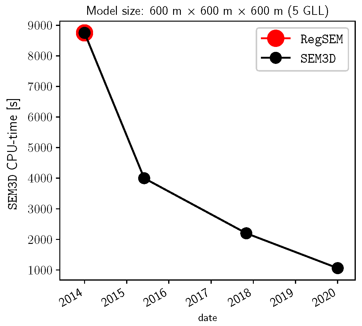
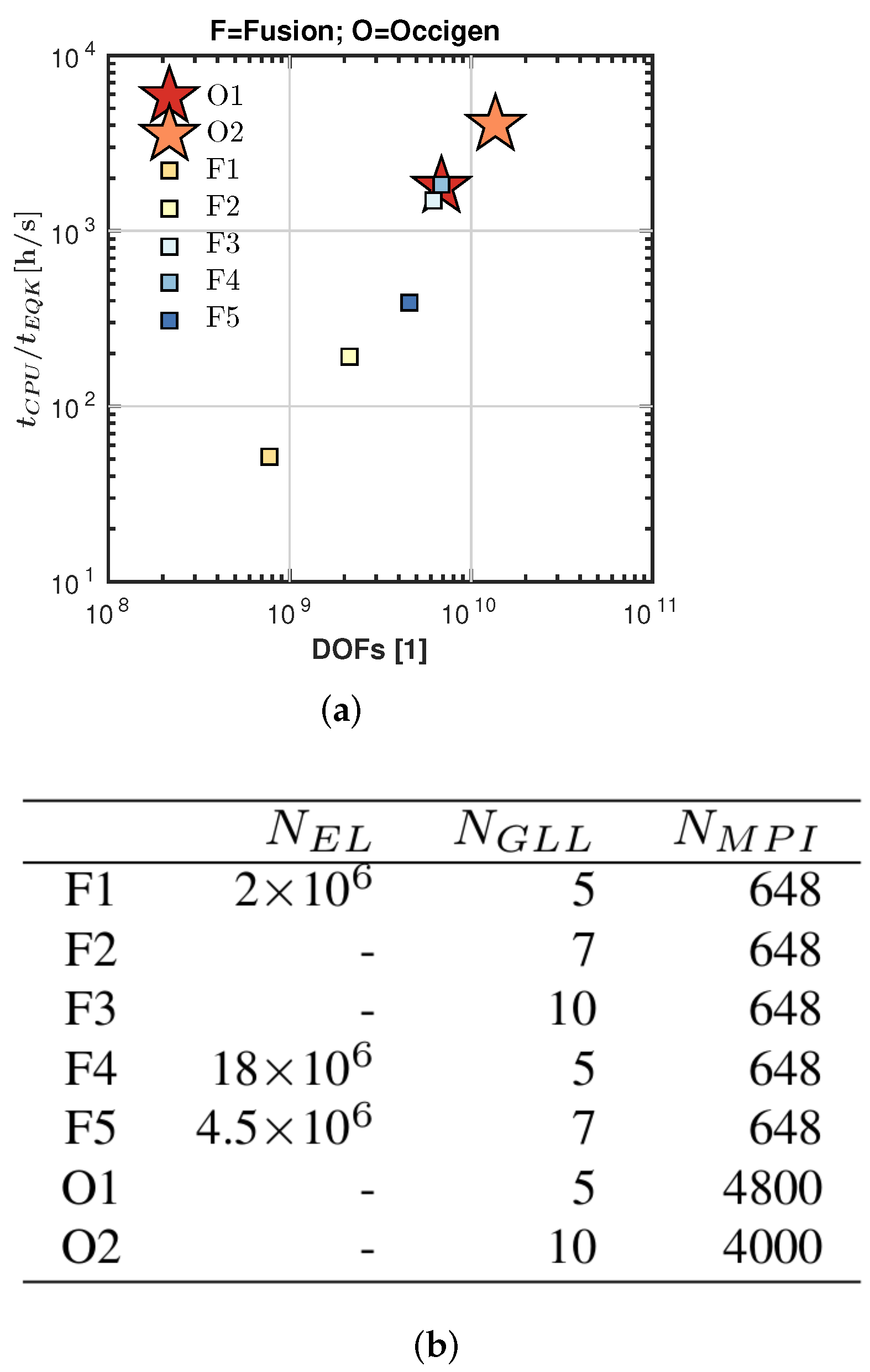
2.2. SEM3D
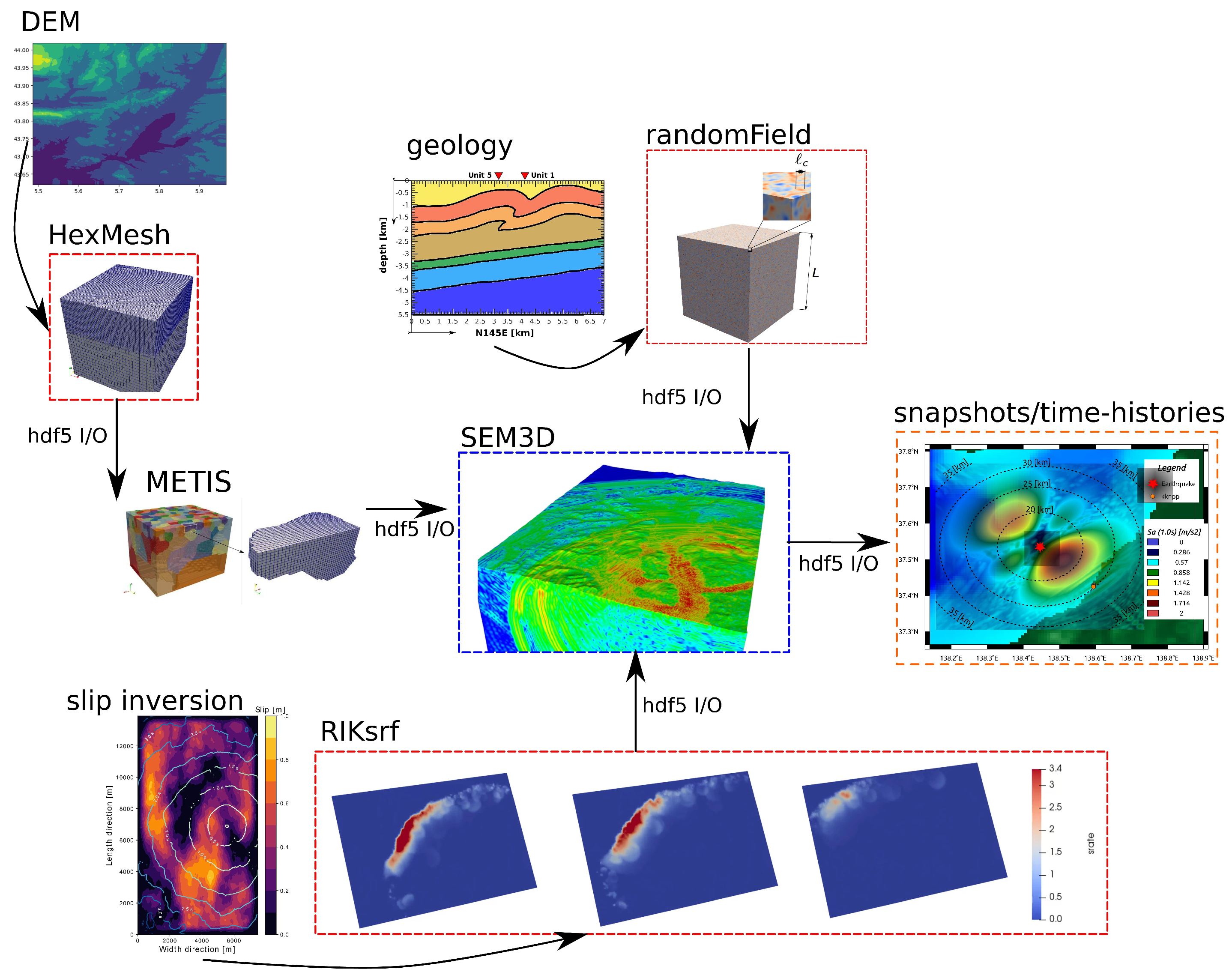
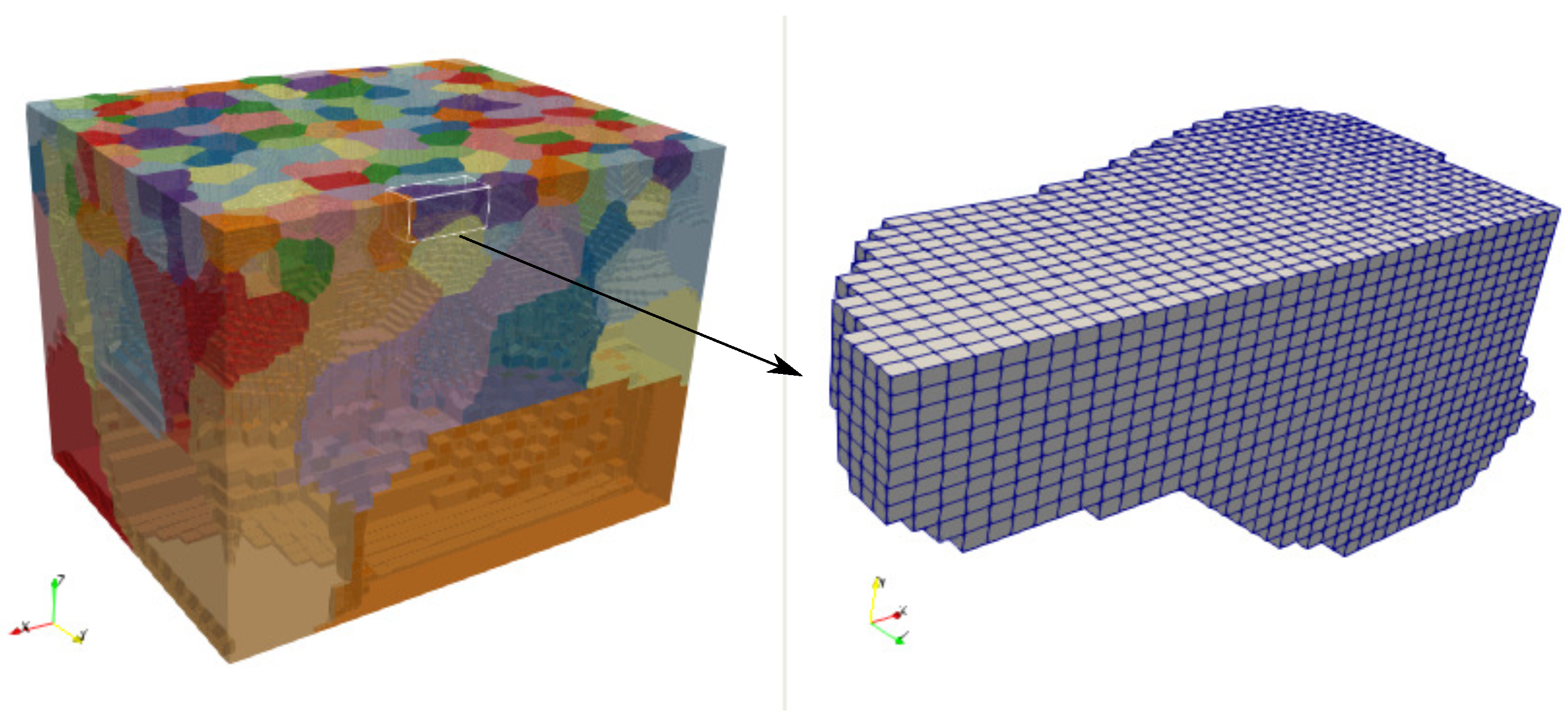
2.3. Meshing Chunks of the Earth’s Crust: HexMesh
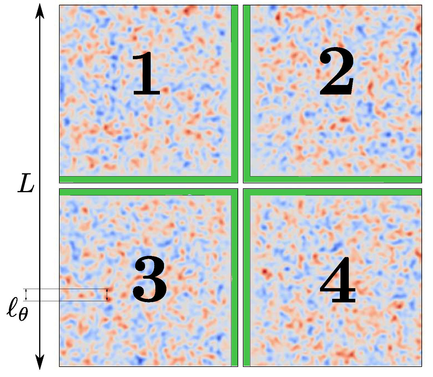
3. Modeling Soil Heterogeneity by Means of Random Field
4. Modeling Extended Seismic Sources
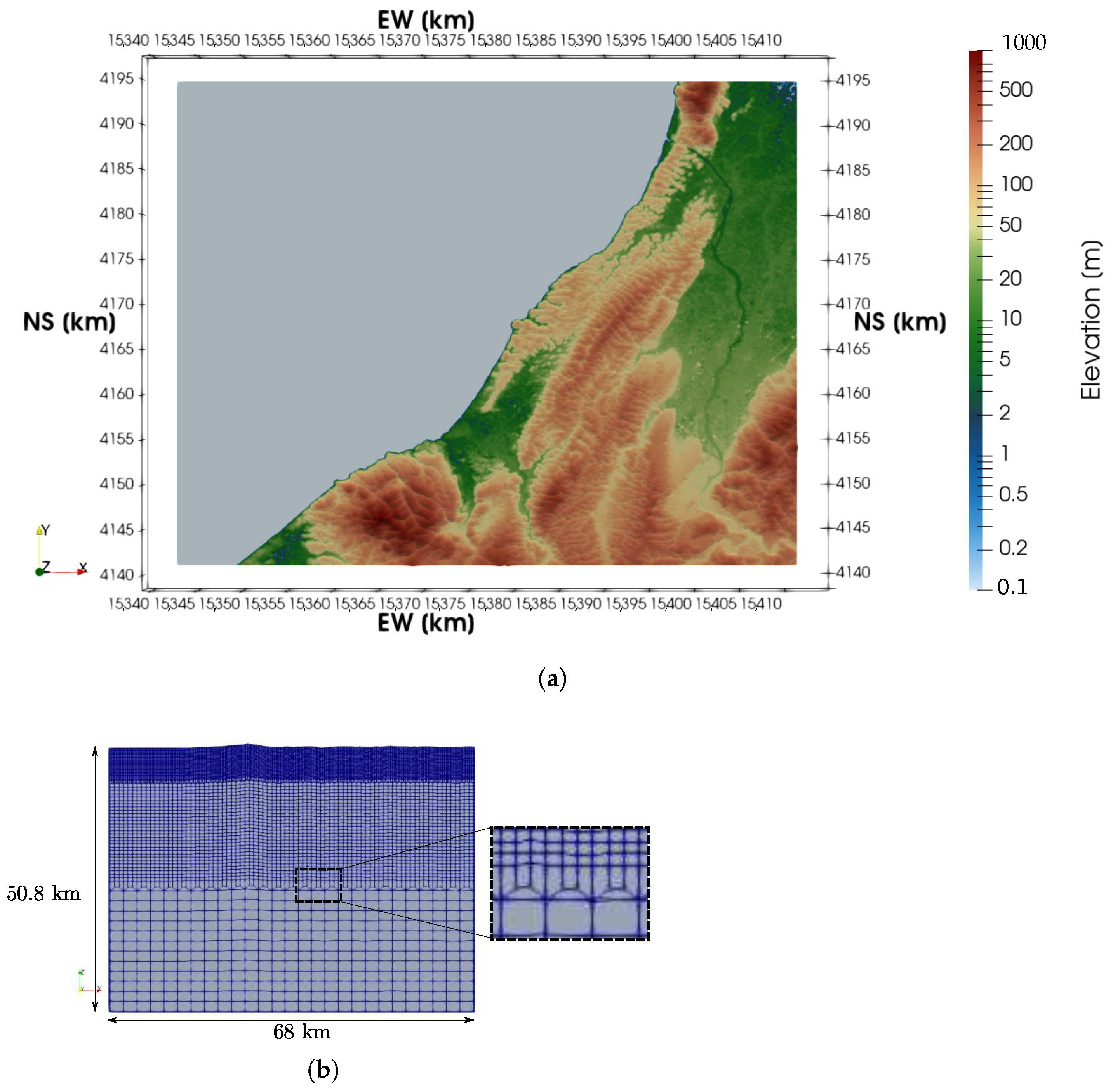
5. Source-to-Site Earthquake Simulation at the Argostoli Site
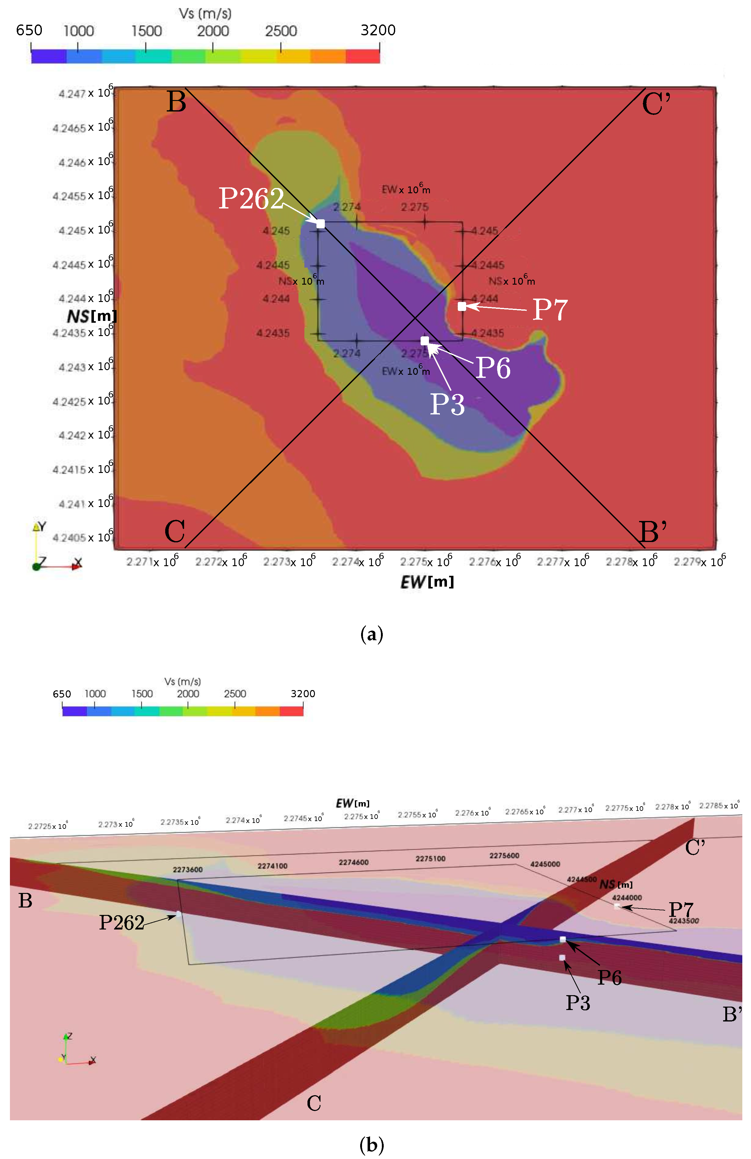
5.1. Geological Characteristics
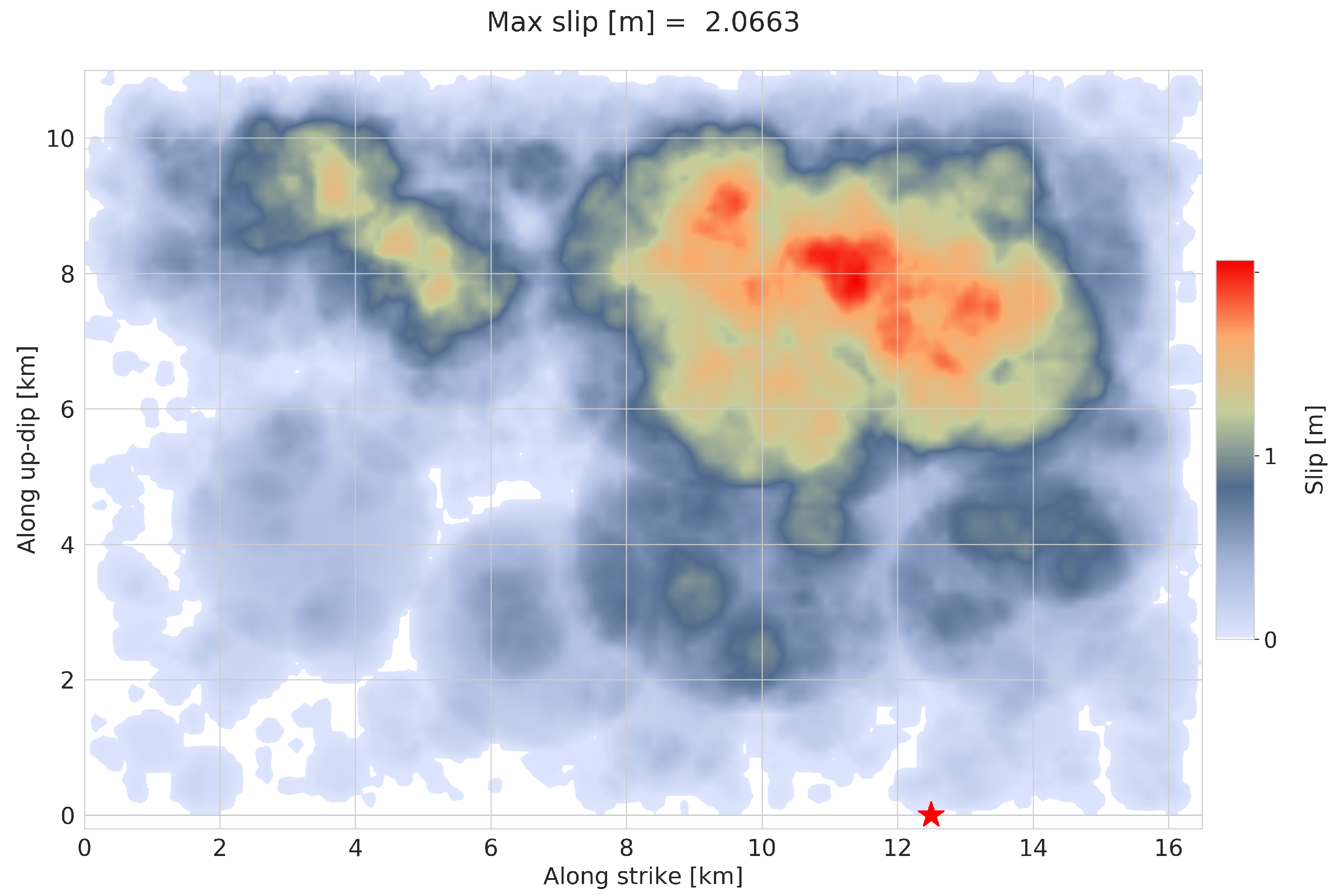
5.2. Seismic Source
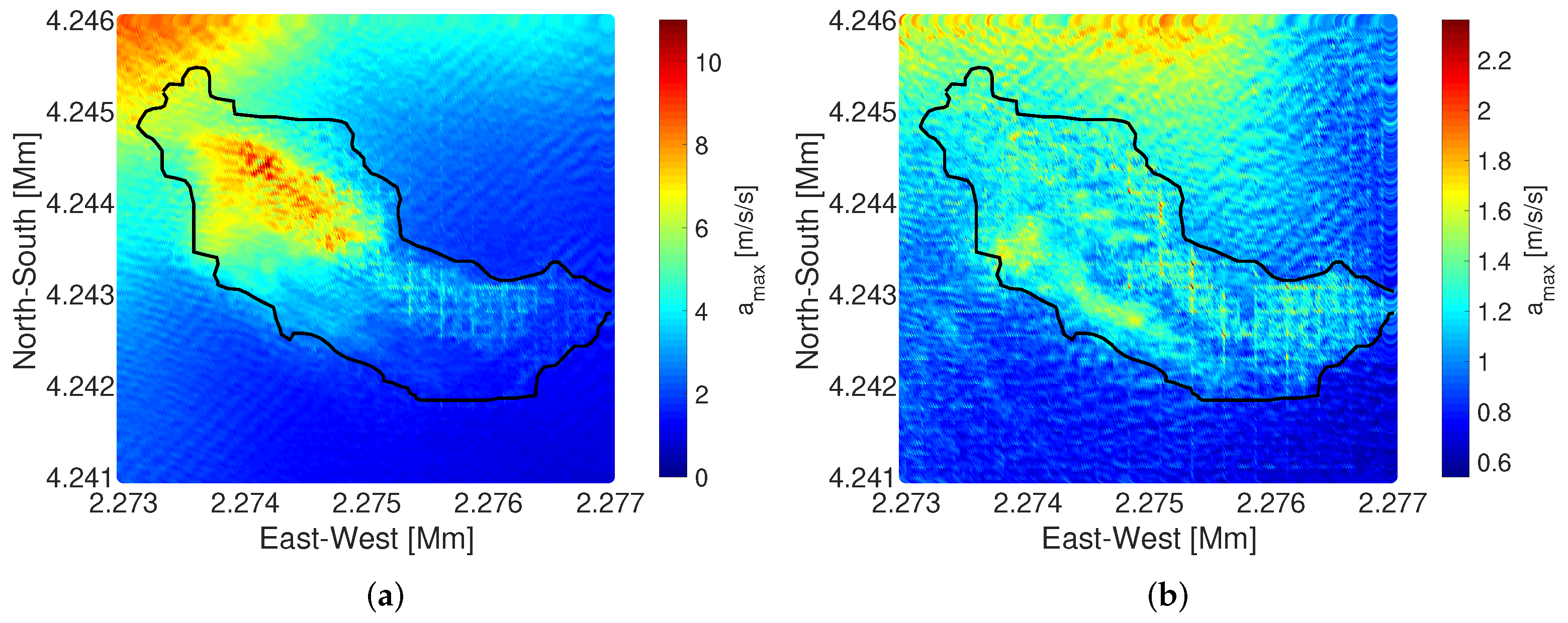
6. Results and Discussion
7. Conclusions
Author Contributions
Funding
Institutional Review Board Statement
Informed Consent Statement
Data Availability Statement
Acknowledgments
Conflicts of Interest
Abbreviations
| 3-D | Three-dimensional |
| BBS2S | Broad-Band Source-to-Site |
| CEA | Commissariat à l’énergie atomique et aux énergies alternatives |
| CFL | Courant–Friedrichs–Lewy |
| CPU | Central Process Unit |
| CoV | Coefficient of Variation |
| DEM | Digital Elevation Model |
| E2VP | EUROSEISTEST Verification and Validation Project |
| DG | Discontinuous Galerkin |
| FDM | Finite-Difference Method |
| FEM | Finite-Element Method |
| G.L. | Ground Level |
| GLL | Gauss–Lobatto–Legendre |
| GMPE | Ground Motion Prediction Equation |
| GPS | Global Positioning System |
| GPU | Graphic Process Unit |
| I/O | Input/Output |
| InSAR | Interferometric synthetic aperture radar |
| IPGP | Institut de Physique du Globe de Paris |
| MPI | Message Passing Interface |
| NERA | Network of European Research Infrastructures for Earthquake Risk Assessment and Mitigation |
| PGA | Peak Ground Acceleration |
| PML | Perfectly Matched Layer |
| PSA | Pseudo Spectral Acceleration |
| RIK | Ruiz Integral Kinematic |
| SEM | Spectral Element Method |
References
- Aki, K.; Richards, P.G. Quantitative Seismology; Books in Geology; W.H Freeman and Company: San Francisco, CA, USA, 2002; Volume I–II. [Google Scholar]
- Aki, K.; Chouet, B. Origin of coda waves: Source, attenuation, and scattering effects. J. Geophys. Res. 1975, 80, 3322–3342. [Google Scholar] [CrossRef]
- Nakano, K.; Matsushima, S.; Kawase, H. Statistical Properties of Strong Ground Motions from the Generalized Spectral Inversion of Data Observed by K-NET, KiK-net, and the JMA Shindokei Network in Japan. Bull. Seismol. Soc. Am. 2015, 105, 2662–2680. [Google Scholar] [CrossRef]
- Mai, P.M.; Beroza, G.C. A spatial random field model to characterize complexity in earthquake slip. J. Geophys. Res. Solid Earth 2002, 107, ESE 10-1–ESE 10-21. [Google Scholar] [CrossRef]
- Aochi, H. Input Ground Motion Calculation Based on Dynamic Rupture Modeling on Segmented Faults. In Proceedings of the International Workshop on Best Practices in Physics-based Fault Rupture Models for Seismic Hazard Assessment of Nuclear Installations, Vienna, Austria, 18–20 November 2015. [Google Scholar]
- Chaljub, E.; Maufroy, E.; Moczo, P.; Kristek, J.; Hollender, F.; Bard, P.Y.; Priolo, E.; Klin, P.; De Martin, F.; Zhang, Z.; et al. 3-D numerical simulations of earthquake ground motion in sedimentary basins: Testing accuracy through stringent models. Geophys. J. Int. 2015, 201, 90–111. [Google Scholar] [CrossRef] [Green Version]
- Moczo, P.; Kristek, J.; Bard, P.Y.; Stripajová, S.; Hollender, F.; Chovanová, Z.; Kristeková, M.; Sicilia, D. Key structural parameters affecting earthquake ground motion in 2D and 3D sedimentary structures. Bull. Earthq. Eng. 2018, 16, 2421–2450. [Google Scholar] [CrossRef] [Green Version]
- De Martin, F.; Chaljub, E.; Thierry, P.; Sochala, P.; Dupros, F.; Maufroy, E.; Hadri, B.; Benaichouche, A.; Hollender, F. Influential parameters on 3-D synthetic ground motions in a sedimentary basin derived from global sensitivity analysis. Geophys. J. Int. 2021, 227, 1795–1817. [Google Scholar] [CrossRef]
- Faccioli, E.; Tagliani, A.; Paolucci, R. Effects of the Wave-Propagation in Random Earth’s Media on the Seismic Radiation Spectra. In Proceedings of the 4th International Conference on Soil Dynamics and Earthquake Engineering, Mexico City, Mexico, 23–26 October 1989; Cakmak, A.S., Herrera, I., Eds.; Computational Mechanics Publications: Berlin, Germany, 1989; pp. 61–75. [Google Scholar]
- Moczo, P.; Kristek, J.; Vavryčuk, V.; Archuleta, R.J.; Halada, L. 3D heterogeneous staggered-grid finite-difference modeling of seismic motion with volume harmonic and arithmetic averaging of elastic moduli and densities. Bull. Seismol. Soc. Am. 2002, 92, 3042–3066. [Google Scholar] [CrossRef]
- Scalise, M.; Pitarka, A.; Louie, J.N.; Smith, K.D. Effect of Random 3D Correlated Velocity Perturbations on Numerical Modeling of Ground Motion from the Source Physics Experiment. Bull. Seismol. Soc. Am. 2021, 111, 139–156. [Google Scholar] [CrossRef]
- Ichimura, T.; Fujita, K.; Quinay, P.E.B.; Maddegedara, L.; Hori, M.; Tanaka, S.; Shizawa, Y.; Kobayashi, H.; Minami, K. Implicit nonlinear wave simulation with 1.08 T DOF and 0.270 T unstructured finite elements to enhance comprehensive earthquake simulation. In Proceedings of the High Performance Computing, Networking, Storage and Analysis, Austin, TX, USA, 15–20 November 2015; pp. 1–12. [Google Scholar] [CrossRef] [Green Version]
- Ichimura, T.; Fujita, K.; Tanaka, S.; Hori, M.; Lalith, M.; Shizawa, Y.; Kobayashi, H. Physics-Based Urban Earthquake Simulation Enhanced by 10.7 BlnDOF x 30 K Time-Step Unstructured FE Non-Linear Seismic Wave Simulation. In Proceedings of the SC ’14: Proceedings of the International Conference for High Performance Computing, Networking, Storage and Analysis, New Orleans, LA, USA, 16–21 November 2014; pp. 15–26. [Google Scholar] [CrossRef]
- Restrepo, D.; Bielak, J.; Serrano, R.; Gomez, J.; Jaramillo, J. Effects of realistic topography on the ground motion of the Colombian Andes—A case study at the Aburrá Valley, Antioquia. Geophys. J. Int. 2016, 204, 1801–1816. [Google Scholar] [CrossRef] [Green Version]
- Ichimura, T.; Fujita, K.; Yoshiyuki, A.; Quinay, P.E.; Hori, M.; Sakanoue, T. Performance Enhancement of Three-Dimensional Soil Structure Model via Optimization for Estimating Seismic Behavior of Buried Pipelines. J. Earthq. Tsunami 2017, 11, 1750019. [Google Scholar] [CrossRef]
- Zuchowski, L.; Brun, M.; De Martin, F. Co-simulation coupling spectral/finite elements for 3D soil/structure interaction problems. C. R. Méc. 2018, 346, 408–422. [Google Scholar] [CrossRef]
- Brun, M.; De Martin, F.; Richart, N. Hybrid asynchronous SEM/FEM co-simulation for seismic nonlinear analysis of concrete gravity dams. Comput. Struct. 2021, 245, 106459. [Google Scholar] [CrossRef]
- Paolucci, R.; Mazzieri, I.; Smerzini, C.; Stupazzini, M. Physics -Based Earthquake Ground Shaking Scenarios in Large Urban Areas. In Perspectives on European Earthquake Engineering and Seismology; Ansal, A., Ed.; Springer: Cham, Switzerland, 2014; Volume 34, pp. 331–359. [Google Scholar]
- Carrington, L.; Komatitsch, D.; Laurenzano, M.; Tikir, M.; Michéa, D.; Le Goff, N.; Snavely, A.; Tromp, J. High-frequency simulations of global seismic wave propagation using SPECFEM3D_GLOBE on 62 thousand processor cores. In Proceedings of the SC’08 ACM/IEEE conference on Supercomputing, Austin, TX, USA, 15–21 November 2008; pp. 1–11. [Google Scholar] [CrossRef]
- Dupros, F.; De Martin, F.; Foerster, E.; Komatitsch, D.; Roman, J. High-performance finite-element simulations of seismic wave propagation in three-dimensional nonlinear inelastic geological media. Parallel Comput. 2010, 36, 308–325. [Google Scholar] [CrossRef] [Green Version]
- Paolucci, R.; Mazzieri, I.; Smerzini, C. Anatomy of strong ground motion: Near-source records and 3D physics-based numerical simulations of the Mw 6.0 May 29 2012 Po Plain earthquake, Italy. Geophys. J. Int. 2015, 203, 2001–2020. [Google Scholar] [CrossRef]
- Smerzini, C.; Pitilakis, K.; Hashemi, K. Evaluation of earthquake ground motion and site effects in the Thessaloniki urban area by 3D finite-fault numerical simulations. Bull. Earthq. Eng. 2017, 15, 787–812. [Google Scholar] [CrossRef]
- Gatti, F.; Lopez-Caballero, F.; Clouteau, D.; Paolucci, R. On the effect of the 3-D regional geology on the seismic design of critical structures: The case of the Kashiwazaki-Kariwa Nuclear Power Plant. Geophys. J. Int. 2018, 213, 1073–1092. [Google Scholar] [CrossRef]
- Poursartip, B.; Fathi, A.; Tassoulas, J.L. Large-scale simulation of seismic wave motion: A review. Soil Dyn. Earthq. Eng. 2020, 129, 105909. [Google Scholar] [CrossRef]
- Paolucci, R.; Infantino, M.; Mazzieri, I.; Özcebe, A.G.; Smerzini, C.; Stupazzini, M. 3D Physics-Based Numerical Simulations: Advantages and Current Limitations of a New Frontier to Earthquake Ground Motion Prediction. The Istanbul Case Study. In Proceedings of the Recent Advances in Earthquake Engineering in Europe: 16th European Conference on Earthquake Engineering, Thessaloniki, Greece, 18–21 June 2018; Volume 46, p. 203. [Google Scholar]
- Dujardin, A.; Causse, M.; Berge-Thierry, C.; Hollender, F. Radiation Patterns Control the Near-Source Ground-Motion Saturation Effect. Bull. Seismol. Soc. Am. 2018, 108, 3398. [Google Scholar] [CrossRef]
- De Martin, F. Verification of a Spectral-Element Method Code for the Southern California Earthquake Center LOH.3 Viscoelastic Case. Bull. Seismol. Soc. Am. 2011, 101, 2855–2865. [Google Scholar] [CrossRef]
- Cupillard, P.; Delavaud, E.; Burgos, G.; Festa, G.; Vilotte, J.P.; Capdeville, Y.; Montagner, J.P. RegSEM: A versatile code based on the spectral element method to compute seismic wave propagation at the regional scale. Geophys. J. Int. 2012, 188, 1203–1220. [Google Scholar] [CrossRef] [Green Version]
- Quinay, P.E.B.; Ichimura, T.; Hori, M.; Nishida, A.; Yoshimura, S. Seismic Structural Response Estimates of a Fault-Structure System Model with Fine Resolution Using Multiscale Analysis with Parallel Simulation of Seismic-Wave Propagation. Bull. Seismol. Soc. Am. 2013, 103, 2094–2110. [Google Scholar] [CrossRef]
- He, C.H.; Wang, J.T.; Zhang, C.H. Nonlinear Spectral-Element Method for 3D Seismic-Wave Propagation. Bull. Seismol. Soc. Am. 2016, 106, 1074–1087. [Google Scholar] [CrossRef]
- Ichimura, T.; Agata, R.; Hori, T.; Hirahara, K.; Hashimoto, C.; Hori, M.; Fukahata, Y. An elastic/viscoelastic finite element analysis method for crustal deformation using a 3-D island-scale high-fidelity model. Geophys. J. Int. 2016, 206, 114–129. [Google Scholar] [CrossRef] [Green Version]
- Tsuboi, S.; Ando, K.; Miyoshi, T.; Peter, D.; Komatitsch, D.; Tromp, J. A 1.8 trillion degrees-of-freedom, 1.24 petaflops global seismic wave simulation on the K computer. Int. J. High Perform. Comput. Appl. 2016, 30, 411–422. [Google Scholar] [CrossRef] [Green Version]
- Baltaji, O.; Numanoglu, O.A.; Veeraraghavan, S.; Hashash, Y.M.; Coleman, J.L.; Bolisetti, C. Non-linear Time Domain Site Response and Soil Structure Analyses for Nuclear Facilities using MASTODON. In Proceedings of the 24th Conference on Structural Mechanics in Reactor Technology, Busan, Korea, 20–25 August 2017. [Google Scholar]
- Ichimura, T.; Fujita, K.; Horikoshi, M.; Meadows, L.; Nakajima, K.; Yamaguchi, T.; Koyama, K.; Inoue, H.; Naruse, A.; Katsushima, K.; et al. A Fast Scalable Implicit Solver with Concentrated Computation for Nonlinear Time-Evolution Problems on Low-Order Unstructured Finite Elements. In Proceedings of the 2018 IEEE International Parallel and Distributed Processing Symposium (IPDPS), Vancouver, BC, Canada, 21–25 May 2018; pp. 620–629. [Google Scholar] [CrossRef]
- Gatti, F.; Touhami, S.; Lopez-Caballero, F.; Paolucci, R.; Clouteau, D.; Alves Fernandes, V.; Kham, M.; Voldoire, F. Broad-band 3-D earthquake simulation at nuclear site by an all-embracing source-to-structure approach. Soil Dyn. Earthq. Eng. 2018, 115, 263–280. [Google Scholar] [CrossRef] [Green Version]
- Casarotti, E.; Stupazzini, M.; Lee, S.; Komatitsch, D.; Piersanti, A.; Tromp, J. CUBIT and seismic wave propagation based upon the spectral-element method: An advanced unstructured mesher for complex 3D geological media. In Proceedings of the 16th International Meshing Roundtable, Seattle, WA, USA, 14–17 October 2007; Volume 5B.4, pp. 579–597. [Google Scholar]
- Gatti, F.; Paludo, L.D.C.; Svay, A.; Lopez-Caballero, F.; Cottereau, R.; Clouteau, D. Investigation of the earthquake ground motion coherence in heterogeneous non-linear soil deposits. Procedia Eng. 2017, 199, 2354–2359. [Google Scholar] [CrossRef]
- Yoshiyuki, A.; Fujita, K.; Ichimura, T.; Hori, M.; Wijerathne, L. Development of Scalable Three-Dimensional Elasto-Plastic Nonlinear Wave Propagation Analysis Method for Earthquake Damage Estimation of Soft Grounds. In Proceedings of the Computational Science—ICCS 2018, Wuxi, China, 11–13 June 2018; Shi, Y., Fu, H., Tian, Y., Krzhizhanovskaya, V.V., Lees, M.H., Dongarra, J., Sloot, P.M.A., Eds.; Springer International Publishing: Cham, Switzerland, 2018; pp. 3–16. [Google Scholar]
- de Carvalho Paludo, L.; Bouvier, V.; Cottereau, R. Scalable parallel scheme for sampling of Gaussian random fields over very large domains. Int. J. Numer. Methods Eng. 2019, 117, 845–859. [Google Scholar] [CrossRef] [Green Version]
- Gallovič, F. Modeling Velocity Recordings of the Mw 6.0 South Napa, California, Earthquake: Unilateral Event with Weak High-Frequency Directivity. Seismol. Res. Lett. 2016, 87, 2–14. [Google Scholar] [CrossRef]
- Pelties, C.; Gabriel, A.A.; Ampuero, J.P. Verification of an ADER-DG method for complex dynamic rupture problems. Geosci. Model Dev. 2014, 7, 847–866. [Google Scholar] [CrossRef] [Green Version]
- CEA and CentraleSupélec and IPGP and CNRS. SEM3D Ver 2017.04 Registered at French Agency for Protection of Programs (Dépôt APP). France IDDN.FR.001.400009.000.S.P.2018.000.31235. 2017. Available online: https://www.researchgate.net/publication/349254101_SEM3D-High-resolution_seismic_wave_propagation_modelling_from_the_fault_to_the_structure_for_realistic_earthquake_scenarios_GENCI_Allocation_A0080410444 (accessed on 24 January 2022).
- Kristek, J.; Moczo, P.; Chaljub, E.; Kristekova, M. An orthorhombic representation of a heterogeneous medium for the finite-difference modelling of seismic wave propagation. Geophys. J. Int. 2016, 208, 1250–1264. [Google Scholar] [CrossRef]
- Cultrera, G.; Andreou, T.; Bard, P.Y.; Boxberger, T.; Cara, F.; Cornou, C.; Di Giulio, G.; Hollender, F.; Imitiaz, A.; Kementzetzidou, D.; et al. The Argostoli (Cephalonia, Greece) experiment. In Proceedings of the Second European Conference on Earthquake Engineering and Seismology (2ECEES), Istanbul, Turkey, 25–29 August 2014; pp. 24–29. [Google Scholar]
- Sokos, E.; Kiratzi, A.; Gallovič, F.; Zahradník, J.; Serpetsidaki, A.; Plicka, V.; Janský, J.; Kostelecký, J.; Tselentis, G. Rupture process of the 2014 Cephalonia, Greece, earthquake doublet (Mw6) as inferred from regional and local seismic data. Tectonophysics 2015, 656, 131–141. [Google Scholar] [CrossRef]
- Theodoulidis, N.; Hollender, F.; Mariscal, A.; Moiriat, D.; Bard, P.Y.; Konidaris, A.; Cushing, M.; Konstantinidou, K.; Roumelioti, Z. The ARGONET (Greece) Seismic Observatory: An Accelerometric Vertical Array and Its Data. Seismol. Res. Lett. 2018, 89, 1555–1565. [Google Scholar] [CrossRef]
- Cushing, E.; Hollender, F.; Guyonnet-Benaize, C.; Perron, V.; Imtiaz, A.; Svay, A.; Mariscal, A.; Bard, P.Y.; Cottereau, R.; Lopez-Caballero, F.; et al. Close to the lair of Odysseus Cyclops: The SINAPS postseismic campaign and accelerometric network installation on Cephalonia island—Site effect characterization experiment. In Proceedings of the 7th International INQUA Meeting on Paleoseismology, Active Tectonics and Archeoseismology (PATA), Crestone, CO, USA, 30 May–3 June 2016. [Google Scholar]
- Svay, A.; Perron, V.; Imtiaz, A.; Zentner, I.; Cottereau, R.; Clouteau1, D.; Bard, P.Y.; Hollender, F.; Lopez-Caballero, F. Spatial coherency analysis of seismic ground motions from a rock site dense array implemented during the Kefalonia 2014 aftershock sequence. Earthq. Eng. Struct. Dyn. 2017, 46, 1895–1917. [Google Scholar] [CrossRef]
- Berge-Thierry, C.; Svay, A.; Laurendeau, A.; Chartier, T.; Perron, V.; Guyonnet-Benaize, C.; Kishta, E.; Cottereau, R.; Lopez-Caballero, F.; Hollender, F.; et al. Toward an integrated seismic risk assessment for nuclear safety improving current French methodologies through the SINAPS@ research project. Nucl. Eng. Des. 2017, 323, 185–201. [Google Scholar] [CrossRef] [Green Version]
- Touhami, S. Numerical Modeling of Seismic Field and Soil Interaction: Application to the Sedimentary Basin of Argostoli (Greece). Ph.D. Thesis, Université Paris Saclay, Gif-sur-Yvette, France, 2020. [Google Scholar]
- Touhami, S.; Lopez-Caballero, F.; Clouteau, D. A holistic approach of numerical analysis of the geology effects on ground motion prediction: Argostoli site test. J. Seismol. 2020, 25, 115–140. [Google Scholar] [CrossRef]
- Bradley, B.A. On-going challenges in physics-based ground motion prediction and insights from the 2010–2011 Canterbury and 2016 Kaikoura, New Zealand earthquakes. Soil Dyn. Earthq. Eng. 2019, 124, 354–364. [Google Scholar] [CrossRef]
- Komatitsch, D.; Vilotte, J.P. The Spectral Element Method: An Efficient Tool to Simulate the Seismic Response of 2D and 3D Geological Structures. Bull. Seismol. Soc. Am. 1998, 88, 368–392. [Google Scholar] [CrossRef]
- Patera, A. A spectral element method for fluid dynamics: Laminar flow in a channel expansion. J. Comput. Phys. 1984, 54, 468–488. [Google Scholar] [CrossRef]
- Korczak, K.Z.; Patera, A.T. An isoparametric spectral element method for solution of the Navier-Stokes equations in complex geometry. J. Comput. Phys. 1986, 62, 361–382. [Google Scholar] [CrossRef]
- Maday, Y.; Patera, A.T.; Ronquist, E.M. A Well-Posed Optimal Spectral Element Approximation for the Stokes Problem; Technical Report, ICASE Report, no. 87-48.; NASA Contractor Report, NASA CR-178343; NASA: Washington, DC, USA, 1987.
- Maday, Y.; Patera, A.; Rønquist, E. Optimal Legendre spectral element methods for the multi-dimensional Stokes problem. SIAM J. Num. Anal. 1989. [Google Scholar]
- Seriani, G. 3-D large-scale wave propagation modeling by spectral element method on Cray T3E multiprocessor. Comput. Methods Appl. Mech. Eng. 1998, 164, 235–247. [Google Scholar] [CrossRef]
- Komatitsch, D.; Tromp, J. Introduction to the spectral element method for three-dimensional seismic wave propagation. Geophys. J. Int. 1999, 139, 806–822. [Google Scholar] [CrossRef]
- Delavaud, E. Simulation Numérique de la Propagation D’ondes en Milieu Géologique Complexe: Application à L’évaluation de la Réponse Sismique du Bassin de Caracas (Venezuela); Institut de Physique du Globe de Paris: Paris, France, 2007. [Google Scholar]
- Mazzieri, I.; Stupazzini, M.; Guidotti, R.; Smerzini, C. SPEED: SPectral Elements in Elastodynamics with Discontinuous Galerkin: A non-conforming approach for 3D multi-scale problems. Int. J. Numer. Methods Eng. 2013, 95, 991–1010. [Google Scholar] [CrossRef]
- Simo, J.; Tarnow, N.; Wong, K. Exact energy-momentum conserving algorithms and symplectic schemes for nonlinear dynamics. Comput. Methods Appl. Mech. Eng. 1992, 100, 63–116. [Google Scholar] [CrossRef]
- Courant, R.; Friedrichs, K.; Lewy, H. On the partial difference equations of mathematical physics. IBM J. Res. Dev. 1967, 11, 215–234. [Google Scholar] [CrossRef]
- Cohen, G.C. High-Order Numerical Methods for Transient Wave Equations; Springer: Berlin, Germany, 2010; Volume 63, p. 49. [Google Scholar] [CrossRef]
- Sevilla, R.; Cottereau, R. Influence of periodically fluctuating material parameters on the stability of explicit high-order spectral element methods. J. Comput. Phys. 2018, 373, 304–323. [Google Scholar] [CrossRef] [Green Version]
- Cottereau, R.; Sevilla, R. Stability of an explicit high-order spectral element method for acoustics in heterogeneous media based on local element stability criteria. Int. J. Numer. Methods Eng. 2018, 116, 223–245. [Google Scholar] [CrossRef]
- Seriani, G.; Oliveira, S.P. Dispersion analysis of spectral element methods for elastic wave propagation. Wave Motion 2008, 45, 729–744. [Google Scholar] [CrossRef]
- Berenger, J.P. A perfectly matched layer for the absorption of electromagnetic waves. J. Comput. Phys. 1994, 114, 185–200. [Google Scholar] [CrossRef]
- Festa, G.; Vilotte, J.P. The Newmark scheme as velocity-stress time-staggering: An efficient PML implementation for spectral element simulations of elastodynamics. Geophys. J. Int. 2005, 161, 789–812. [Google Scholar] [CrossRef]
- Chaljub, E.; Komatitsch, D.; Vilotte, J.P.; Capdeville, Y.; Valette, B.; Festa, G. Spectral-element analysis in seismology. Adv. Geophys. 2007, 48, 365–419. [Google Scholar]
- Chabot, S.; Glinsky, N.; Diego Mercerat, E.; Bonilla, L.F. A High-Order Discontinuous Galerkin Method for Coupled Wave Propagation in 1D Elastoplastic Heterogeneous Media. J. Theor. Comput. Acoust. 2018, 26, 1850043. [Google Scholar] [CrossRef]
- Sornet, G.; Jubertie, S.; Dupros, F.; De Martin, F.; Limet, S. Performance Analysis of SIMD Vectorization of High-Order Finite-Element Kernels. In Proceedings of the 2018 International Conference on High Performance Computing Simulation (HPCS), Orleans, France, 16–20 July 2018; pp. 423–430. [Google Scholar] [CrossRef] [Green Version]
- Tang, H.; Byna, S.; Petersson, N.A.; McCallen, D. Tuning Parallel Data Compression and I/O for Large-scale Earthquake Simulation. In Proceedings of the 2021 IEEE International Conference on Big Data (Big Data), Orlando, FL, USA, 15–18 December 2021; pp. 2992–2997. [Google Scholar] [CrossRef]
- Göddeke, D.; Komatitsch, D.; Möller, M. Finite and Spectral Element Methods on Unstructured Grids for Flow and Wave Propagation Problems. In Numerical Computations with GPUs; Springer International Publishing: Berlin, Germany, 2014; pp. 183–206. [Google Scholar] [CrossRef]
- Markall, G.R.; Slemmer, A.; Ham, D.A.; Kelly, P.H.J.; Cantwell, C.D.; Sherwin, S.J. Finite element assembly strategies on multi-core and many-core architectures. Int. J. Numer. Methods Fluids 2013, 71, 80–97. [Google Scholar] [CrossRef]
- Lombard, B.; Piraux, J. Numerical modeling of transient two-dimensional viscoelastic waves. J. Comput. Phys. 2011, 230, 6099–6114. [Google Scholar] [CrossRef] [Green Version]
- Fu, H.; He, C.; Chen, B.; Yin, Z.; Zhang, Z.; Zhang, W.; Zhang, T.; Xue, W.; Liu, W.; Yin, W.; et al. 18.9Pflopss Nonlinear Earthquake Simulation on Sunway TaihuLight: Enabling Depiction of 18-Hz and 8-meter Scenarios. In Proceedings of the International Conference for High Performance Computing, Networking, Storage and Analysis, New York, NY, USA, 12–17 November 2017; pp. 2:1–2:12. [Google Scholar] [CrossRef]
- Chaljub, E.; Moczo, P.; Tsuno, S.; Bard, P.Y.; Kristek, J.; Käser, M.; Stupazzini, M.; Kristekova, M. Quantitative comparison of four numerical predictions of 3D ground motion in the Grenoble Valley, France. Bull. Seismol. Soc. Am. 2010, 100, 1427–1455. [Google Scholar] [CrossRef]
- Bielak, J.; Graves, R.W.; Olsen, K.B.; Taborda, R.; Ramirez-Guzman, L.; Day, S.M.; Ely, G.; Roten, D.; Jordan, T.; Maechling, P.; et al. The ShakeOut earthquake scenario: Verification of three simulation sets. Geophys. J. Int. 2010, 180, 375–404. [Google Scholar] [CrossRef] [Green Version]
- Komatitsch, D.; Göddeke, D.; Erlebacher, G.; Michéa, D. Modeling the propagation of elastic waves using spectral elements on a cluster of 192 GPUs. Comput. Sci. Res. Dev. 2010, 25, 75–82. [Google Scholar] [CrossRef]
- Cui, Y.; Olsen, K.B.; Jordan, T.H.; Lee, K.; Zhou, J.; Small, P.; Roten, D.; Ely, G.; Panda, D.K.; Chourasia, A.; et al. Scalable earthquake simulation on petascale supercomputers. In Proceedings of the SC ’10: Proceedings of the 2010 ACM/IEEE International Conference for High Performance Computing, Networking, Storage and Analysis, New Orleans, LA, USA, 13–19 November 2010; pp. 1–20. [Google Scholar]
- Rietmann, M.; Messmer, P.; Nissen-Meyer, T.; Peter, D.; Basini, P.; Komatitsch, D.; Schenk, O.; Tromp, J.; Boschi, L.; Giardini, D. Forward and adjoint simulations of seismic wave propagation on emerging large-scale GPU architectures. In Proceedings of the SC ’12: Proceedings of the International Conference on High Performance Computing, Networking, Storage and Analysis, Salt Lake City, UT, USA, 10–16 November 2012; pp. 1–11. [Google Scholar] [CrossRef]
- Taborda, R.; Bielak, J. Ground-Motion Simulation and Validation of the 2008 Chino Hills, California, Earthquake. Bull. Seismol. Soc. Am. 2013, 103, 131–156. [Google Scholar] [CrossRef]
- Heinecke, A.; Breuer, A.; Rettenberger, S.; Bader, M.; Gabriel, A.; Pelties, C.; Bode, A.; Barth, W.; Liao, X.; Vaidyanathan, K.; et al. Petascale High Order Dynamic Rupture Earthquake Simulations on Heterogeneous Supercomputers. In Proceedings of the SC ’14: Proceedings of the International Conference for High Performance Computing, Networking, Storage and Analysis, New Orleans, LA, USA, 16–21 November 2014; pp. 3–14. [Google Scholar] [CrossRef]
- Ichimura, T.; Fujita, K.; Koyama, K.; Kusakabe, R.; Kikuchi, Y.; Hori, T.; Hori, M.; Maddegedara, L.; Ohi, N.; Nishiki, T.; et al. 152K-Computer-Node Parallel Scalable Implicit Solver for Dynamic Nonlinear Earthquake Simulation. In Proceedings of the International Conference on High Performance Computing in Asia-Pacific Region, New York, NY, USA, 12–14 January 2022; pp. 18–29. [Google Scholar] [CrossRef]
- Duru, K.; Rannabauer, L.; Gabriel, A.A.; Ling, O.K.A.; Igel, H.; Bader, M. A stable discontinuous Galerkin method for linear elastodynamics in 3D geometrically complex elastic solids using physics based numerical fluxes. Comput. Methods Appl. Mech. Eng. 2022, 389, 114386. [Google Scholar] [CrossRef]
- Bachem, A. PRACE—Strategy for HPC in Europe; Technical Report; Forschungszentrum Jülich: Jülich, Germany, 2008. [Google Scholar]
- Camata, J.J.; Coutinho, A.L.G.A. Parallel implementation and performance analysis of a linear octree finite element mesh generation scheme. Concurr. Comput. Pract. Exp. 2013, 25, 826–842. [Google Scholar] [CrossRef]
- Shinozuka, M.; Deodatis, G. Simulation of stochastic processes by spectral representation. Appl. Mech. Rev. 1991, 44, 191–204. [Google Scholar] [CrossRef]
- Shinozuka, M.; Deodatis, G. Simulation of multi-dimensional Gaussian stochastic fields by spectral representation. Appl. Mech. Rev. 1996, 49, 29–53. [Google Scholar] [CrossRef]
- Crempien, J.G.F.; Archuleta, R.J. UCSB Method for Simulation of Broadband Ground Motion from Kinematic Earthquake Sources. Seismol. Res. Lett. 2015, 86, 61–67. [Google Scholar] [CrossRef]
- Ruiz, J.A.; Baumont, D.; Bernard, P.; Berge-Thierry, C. Modelling directivity of strong ground motion with a fractal, k-2, kinematic source model. Geophys. J. Int. 2011, 186, 226. [Google Scholar] [CrossRef] [Green Version]
- Eshelby, J.D. The Determination of the Elastic Field of an Ellipsoidal Inclusion, and Related Problems. Proc. R. Soc. Lond. Math. Phys. Eng. Sci. 1957, 241, 376–396. [Google Scholar] [CrossRef]
- Faccioli, E.; Maggio, F.; Paolucci, R.; Quarteroni, A. 2D and 3D elastic wave propagation by a pseudo-spectral domain decomposition method. J. Seismol. 1997, 1, 237–251. [Google Scholar] [CrossRef]
- Louvari, E.; Kiratzi, A.; Papazachos, B. The Cephalonia Transform Fault and its extension to western Lefkada Island (Greece). Tectonophysics 1999, 308, 223–236. [Google Scholar] [CrossRef]
- Saltogianni, V.; Moschas, F.; Stiros, S. The 2014 Cephalonia Earthquakes: Finite Fault Modeling, Fault Segmentation, Shear and Thrusting at the NW Aegean Arc (Greece). Pure Appl. Geophys. 2018, 175, 4145–4164. [Google Scholar] [CrossRef]
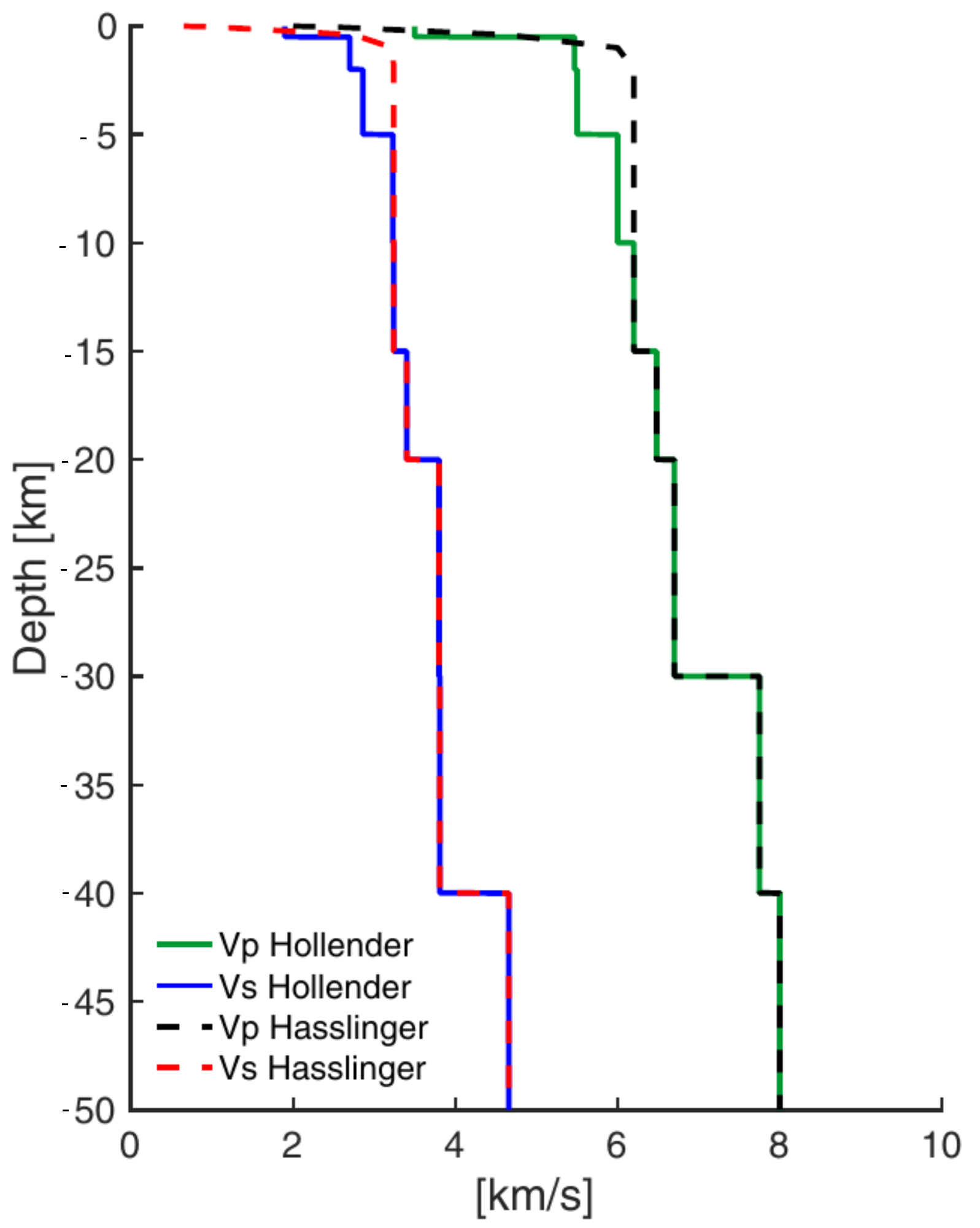
- Haslinger, F.; Kissling, E.; Ansorge, J.; Hatzfeld, D.; Papadimitriou, E.; Karakostas, V.; Makropoulos, K.; Kahle, H.G.; Peter, Y. 3D crustal structure from local earthquake tomography around the Gulf of Arta (Ionian region, NW Greece). Tectonophysics 1999, 304, 201–218. [Google Scholar] [CrossRef]
- Hollender, F.; Perron, V.; Imtiaz, A.; Svay, A.; Mariscal, A.; Bard, P.; Cottereau, R.; Lopez-Caballero, F.; Cushing, M.; Theodoulidis, N.; et al. A Deux Pas du Repaire du Cyclope D’Ulysse: La Campagne Post-Sismique et le Démarrage du Réseau Accélérométrique SINAPS@ sur l’île de Céphalonie; Colloque AFPS: Paris, France, 2015. [Google Scholar]
- Cushing, E.M.; Hollender, F.; Moiriat, D.; Guyonnet-Benaize, C.; Theodoulidis, N.; Pons-Branchu, E.; Sépulcre, S.; Bard, P.Y.; Cornou, C.; Dechamp, A.; et al. Building a three dimensional model of the active Plio-Quaternary basin of Argostoli (Cephalonia Island, Greece): An integrated geophysical and geological approach. Eng. Geol. 2020, 265, 105441. [Google Scholar] [CrossRef]
- Sokos, E.; Zahradnik, J.; Gallovic, F.; Serpetsidaki, A.; Plicka, V.; Kiratzi, A. Asperity break after 12 years: The Mw6.4 2015 Lefkada (Greece) earthquake. Geophys. Res. Lett. 2016, 43, 6137–6145. [Google Scholar] [CrossRef] [Green Version]
- Perron, V.; Hollender, F.; Froment, B.; Gelis, C.; Cushing, E.M.; Bard, P.Y.; Cultrera, G. Can broad-band earthquake site responses be predicted by the ambient noise spectral ratio? Insight from observations at two sedimentary basins. Geophys. J. Int. 2018, 215, 1442–1454. [Google Scholar] [CrossRef]
- Maufroy, E.; Chaljub, E.; Hollender, F.; Kristek, J.; Moczo, P.; Klin, P.; Priolo, E.; Iwaki, A.; Iwata, T.; Etienne, V.; et al. Earthquake Ground Motion in the Mygdonian Basin, Greece: The E2VP Verification and Validation of 3D Numerical Simulation up to 4 Hz. Bull. Seismol. Soc. Am. 2015, 105, 1398–1418. [Google Scholar] [CrossRef] [Green Version]
- Maufroy, E.; Chaljub, E.; Theodoulidis, N.P.; Roumelioti, Z.; Hollender, F.; Bard, P.Y.; de Martin, F.; Guyonnet-Benaize, C.; Margerin, L. Source-Related Variability of Site Response in the Mygdonian Basin (Greece) from Accelerometric Recordings and 3D Numerical Simulations. Bull. Seismol. Soc. Am. 2017, 107, 787–808. [Google Scholar] [CrossRef]
- Akkar, S.; Sandıkkaya, M.A.; Bommer, J.J. Empirical ground-motion models for point- and extended-source crustal earthquake scenarios in Europe and the Middle East. Bull. Earthq. Eng. 2014, 12, 359–387. [Google Scholar] [CrossRef] [Green Version]
- Berge-Thierry, C.; Voldoire, F.; Ragueneau, F.; Lopez-Caballero, F.; Le Maoult, A. Main Achievements of the Multidisciplinary SINAPS Research Project: Towards an Integrated Approach to Perform Seismic Safety Analysis of Nuclear Facilities. Pure Appl. Geophys. 2019, 177, 2299–2351. [Google Scholar] [CrossRef] [Green Version]
- Jussila, V.; Fälth, B.; Mäntyniemi, P.; Voss, P.H.; Lund, B.; Fülöp, L. Application of a Hybrid Modeling Method for Generating Synthetic Ground Motions in Fennoscandia, Northern Europe. Bull. Seismol. Soc. Am. 2021, 111, 2507–2526. [Google Scholar] [CrossRef]
- Oliveira, S.P. Error Analysis of Chebyshev Spectral Element Methods for the Acoustic Wave Equation in Heterogeneous Media. J. Theor. Comput. Acoust. 2018, 26, 1850035. [Google Scholar] [CrossRef]


| Ref. | Year | Method | Ressources | DOFs | Grid Size (m) | Size (km × km × km) | fmax (Hz) | Topography |
|---|---|---|---|---|---|---|---|---|
| [78] | 2010 | FDM | 6 cores | - | 25/125 | - | 2.5 | no |
| 2010 | SEM | 32 cores | 66,187,872 | 150 | - | 2.0 | yes | |
| 2010 | SEM | 63 cores | 39,902,676 | 20–900 | - | 3.0 | yes | |
| 2010 | DG | 510 cores | - | 200–5000 | - | 3.0 | yes | |
| [79] | 2010 | FEM | - | 251,457,147 | var | 600 × 300 × 80 | 0.5 | no |
| 2010 | FDM | - | 2.355 billions | 200 | 500 × 250 × 50 | 0.5 | no | |
| 2010 | FDM | - | 5.419 billions | 100 | 600 × 300 × 80 | 0.5 | no | |
| [80] | 2010 | SEM | 192 GPU | 131,000,256 | - | chunk of earth | 0.7 | no |
| [81] | 2010 | FDM | 1308 billions | 40 | 810 × 405 × 85 | 2.0 | no | |
| [82] | 2012 | SEM | 896 GPU | 22 billions | 24,000 | Western Europe × 200 | 0.125 | yes |
| [83] | 2013 | FEM | 24,000 cores | 15.9 billions | 5.5 88 | 180 × 135 × 32 | 4.0 | no |
| [84] | 2014 | DG | 1,400,832 cores | 96 billions | - | - | 10 | yes |
| [13] | 2017 | FEM | 2,94,912 cores | 10.7 billions | 0.66 | 2 × 2 × 0.1 | - | yes |
| [77] | 2017 | FDM | 1,014,000 cores | 23.4 trillions | 8 | 320 × 312 × 40 | 18 | yes |
| [85] | 2021 | FEM | 1,179,648 cores | 324 billions | 0.125/64 | 256 × 205 × 100 | - | yes |
| This paper | 2022 | SEM | 4000 cores | 13.5 billions | 35 130 | 44 × 44 × 63 | 10 | no |
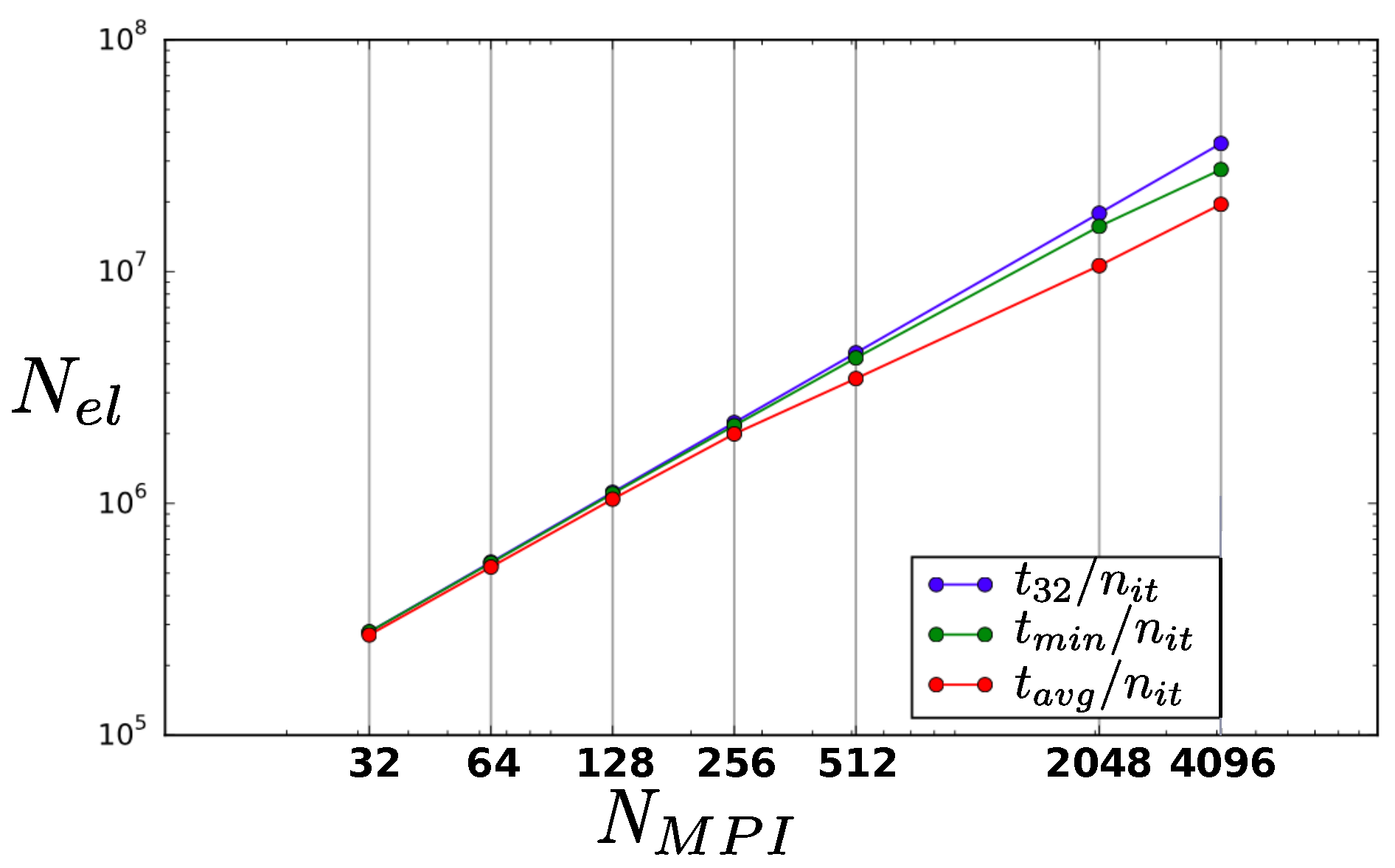
| Cores | Nodes | Generation Time (s) | |
|---|---|---|---|
| Standard | Localized | ||
| 16 | 0.86 | 6.57 | |
| 32 | 1.55 | 13.87 | |
| 256 | 356.43 | 159.98 | |
| 2048 | – | 2037.48 | |
| 4096 | – | 3299.04 | |
| (m) | (m/s) | (m/s) | (1) | (1) |
|---|---|---|---|---|
| 0 | 2000 | 600 | 300 | 150 |
| 300 | 2400 | 1000 | 300 | 150 |
| 400 | 4600 | 2700 | 300 | 150 |
| 1000 | 6000 | 3200 | 300 | 150 |
| 2000 | 6200 | 3200 | 300 | 150 |
Publisher’s Note: MDPI stays neutral with regard to jurisdictional claims in published maps and institutional affiliations. |
© 2022 by the authors. Licensee MDPI, Basel, Switzerland. This article is an open access article distributed under the terms and conditions of the Creative Commons Attribution (CC BY) license (https://creativecommons.org/licenses/by/4.0/).
Share and Cite
Touhami, S.; Gatti, F.; Lopez-Caballero, F.; Cottereau, R.; de Abreu Corrêa, L.; Aubry, L.; Clouteau, D. SEM3D: A 3D High-Fidelity Numerical Earthquake Simulator for Broadband (0–10 Hz) Seismic Response Prediction at a Regional Scale. Geosciences 2022, 12, 112. https://0-doi-org.brum.beds.ac.uk/10.3390/geosciences12030112
Touhami S, Gatti F, Lopez-Caballero F, Cottereau R, de Abreu Corrêa L, Aubry L, Clouteau D. SEM3D: A 3D High-Fidelity Numerical Earthquake Simulator for Broadband (0–10 Hz) Seismic Response Prediction at a Regional Scale. Geosciences. 2022; 12(3):112. https://0-doi-org.brum.beds.ac.uk/10.3390/geosciences12030112
Chicago/Turabian StyleTouhami, Sara, Filippo Gatti, Fernando Lopez-Caballero, Régis Cottereau, Lúcio de Abreu Corrêa, Ludovic Aubry, and Didier Clouteau. 2022. "SEM3D: A 3D High-Fidelity Numerical Earthquake Simulator for Broadband (0–10 Hz) Seismic Response Prediction at a Regional Scale" Geosciences 12, no. 3: 112. https://0-doi-org.brum.beds.ac.uk/10.3390/geosciences12030112