Communication

Evaluation of InfraRed Thermography Supported by UAV and Field Surveys for Rock Mass Characterization in Complex Settings

by
Lidia Loiotine
1,2,*,
Gioacchino Francesco Andriani
2,
Marc-Henri Derron
1,
Mario Parise
2 and
Michel Jaboyedoff
1
1
Institute of Earth Sciences, University of Lausanne, 1015 Lausanne, Switzerland
2
Department of Earth and Environmental Sciences, University of Bari Aldo Moro, 70125 Bari, Italy
*
Author to whom correspondence should be addressed.
Submission received: 11 January 2022 / Revised: 21 February 2022 / Accepted: 28 February 2022 / Published: 2 March 2022
(This article belongs to the Section Geomechanics)

Abstract

:
The InfraRed Thermography (IRT) technique is gaining increasing popularity in the geosciences. Although several studies on the use of this technique for rock mass characterization were reported in the literature, its applicability is challenging in complex environments, characterized by poor accessibility, lithological heterogeneity, karst features and disturbances, such as vegetation and human activities. This paper reports the results of specific tests carried out to explore the application of IRT methods, supported by UAV surveys, for rock mass characterization in complex conditions. In detail, a 24-h monitoring was performed on an appropriate case study to assess which type of information can be collected and what issues can be expected. The results of the thermograms were compared with data reported in the literature and discussed. A novel method to detect correlations between the temperature profiles at the air-rock interfaces and the rock mass properties is presented. The main advantages, limitations and suggestions in order to take full advantage of the IRT technique in complex conditions are reported in the final section.

1. Introduction

InfraRed Thermography (IRT) is a contactless and non-invasive technique measuring the infrared radiations emitted by objects in the form of electronic signal [1] that has recently been gaining popularity in geosciences. Thermal radiation operates in the portion of the electromagnetic spectrum with wavelengths falling in the range of 0.78–1000 μm [1,2,3] (Figure 1). Thermographic cameras are devices working in the wavelength range of 7.15 to 14 μm that measure radiations emitted by objects and convert them into temperatures. The objects investigated by means of IRT techniques provide radiations proportionally to their emissivity ε, which is defined as the ability of an object to emit heat energy [4]. Since the target object itself can reflect radiations emitted by the surrounding objects, part of the total radiation can be dispersed and emitted by the atmosphere [3,5,6]. Hence, the radiation Uobj emitted by the target object and received by a thermographic camera is defined as [3]:
U obj = 1 ε τ U tot 1 ε ε U refl 1 τ τ ε U atm
where ε is the emissivity, τ is the transmittance of the atmosphere, Utot is the total energy received by the thermograph, Urefl is the reflected radiation, and Uatm is the radiation emitted by the atmosphere.
In the last decade, there has been a significant increase in the application of terrestrial and airborne IRT technique, supported by other remote sensing technologies, in geosciences. For instance, thermal cameras, often coupled with LiDAR (Light Detection And Ranging) or UAV (Unmanned Aerial Vehicle) systems, were used to map thermal anomalies of volcanic systems to monitor and predict potential changes [8,9], for landslide mapping [10,11,12,13] and to detect the rock bridges contributing to cliff stability [14]. In addition, thermal cameras were used in mining engineering and cave exploration to identify loose rock blocks, open cracks, tension fractures, high-stress zones, and potential rockfall source areas [7,12,15,16].
Recently, the IRT technique has been widely used for rock mass characterization to study the thermal behavior of rocks under heating and cooling conditions [17,18,19], to detect discontinuity planes, weathered and intensely jointed zones, unstable protruding blocks and water seepage [11,17,20,21,22,23,24,25,26,27,28], according to the contrast of the emitted thermal energy. Thermal devices were coupled with the GPR (Ground Penetration Radar) technique to identify eroded caves behind shotcrete-protected slopes [29]. Being a non-destructive technique, the IRT was used during post-rockfall emergency surveys to evaluate potential reactivations through the detection of fractures and caves [30] and as support for landslide mapping [10], monitoring and early warning [31].
The use of infrared thermography was also extended to geotechnical applications: for instance, the relation between the cooling index of rocks and the compressive strength of rock blocks was identified by coupling IRT and Schmidt Hammer tests [32]. In addition, methods to estimate the porosity of rock samples [33], to predict cracks development [34], wedge indentation [35] and to detect microstructural changes [36] at the laboratory scale were recently proposed.
The generation of 3-D thermal point clouds by means of photogrammetry and Structure from Motion (SfM) approaches was introduced in [37,38] and, despite the low resolution of thermal images compared to other remote sensing techniques, the outputs provided accurate measurements of the rock temperatures for rock mass monitoring. In addition, the inspection of georeferenced 3-D thermal models allows geoscientists not only to extract the main discontinuity sets of rock masses, but also to estimate geomechanical parameters, such as fracture aperture, persistence and weathering degree of rock masses, as demonstrated in [38].
All of the above illustrate several methodologies to perform rock mass characterization at different scales by combining the infrared thermography with other remote sensing technologies (mostly LiDAR and photogrammetry). However, success in large-scale investigations is not guaranteed in poor-accessible sites, especially when only a few shooting points are available. In these circumstances, the field of view and the spatial resolution of the surveyed area are subjected to logistical constraints [25,26,27] and the acquisition of thermal images from short distances and different perspectives to produce high-resolution point clouds is not always possible.
In this study, we present the results of a 24-h monitoring by means of infrared thermography on a rock cliff located in an urban, highly touristic, coastal site, characterized by vertical and lateral lithological heterogeneity, as well as by the presence of karst features. As a matter of fact, the mentioned factors proved to be disturbance elements during previous studies carried out on the same area by means of Terrestrial Laser Scanning (TLS) and UAV technologies for rock mass characterization and rockfall detection [39]. At the same time, the shrubs diffused throughout the rock mass, the artificial cavities and walls, as well as people moving in the field of view, perturbate the thermal outputs of the target in the form of thermal anomalies.
This research is aimed at further investigating the applicability of the IRT technique for large-scale rock mass characterization and to assess whether, in complex conditions, it is possible to derive the information presented in the literature. Indeed, the lithological heterogeneity and the abovementioned disturbance elements represent a challenge for the success in IRT surveys because of the limited spatial resolution related to the site-morphological constraints. Although from a distance sensor-target of 35 m, the ground resolution of the thermal outputs was 2.4 cm, the low resolution of the RGB integrated camera (5 Mpixels) did not allow an appropriate interpretation of the thermal outputs. For this reason, UAV data, field surveys and laboratory tests were carried out to support the IRT processing and interpretation, by directly inspecting the high-resolution photos and the point cloud, and taking into account the material properties (e.g., porosity).
The results of the thermal outputs (both derived from the thermograms and from direct measurements by means of k-type thermocouples) are in agreement with scientific research carried out on other case studies. A novel methodology to directly correlate the air-rock temperatures and the geomorphological, lithological and geostructural setting of rock masses through the alignment of profiles extracted from thermal images and point clouds is presented.

2. Materials and Methods

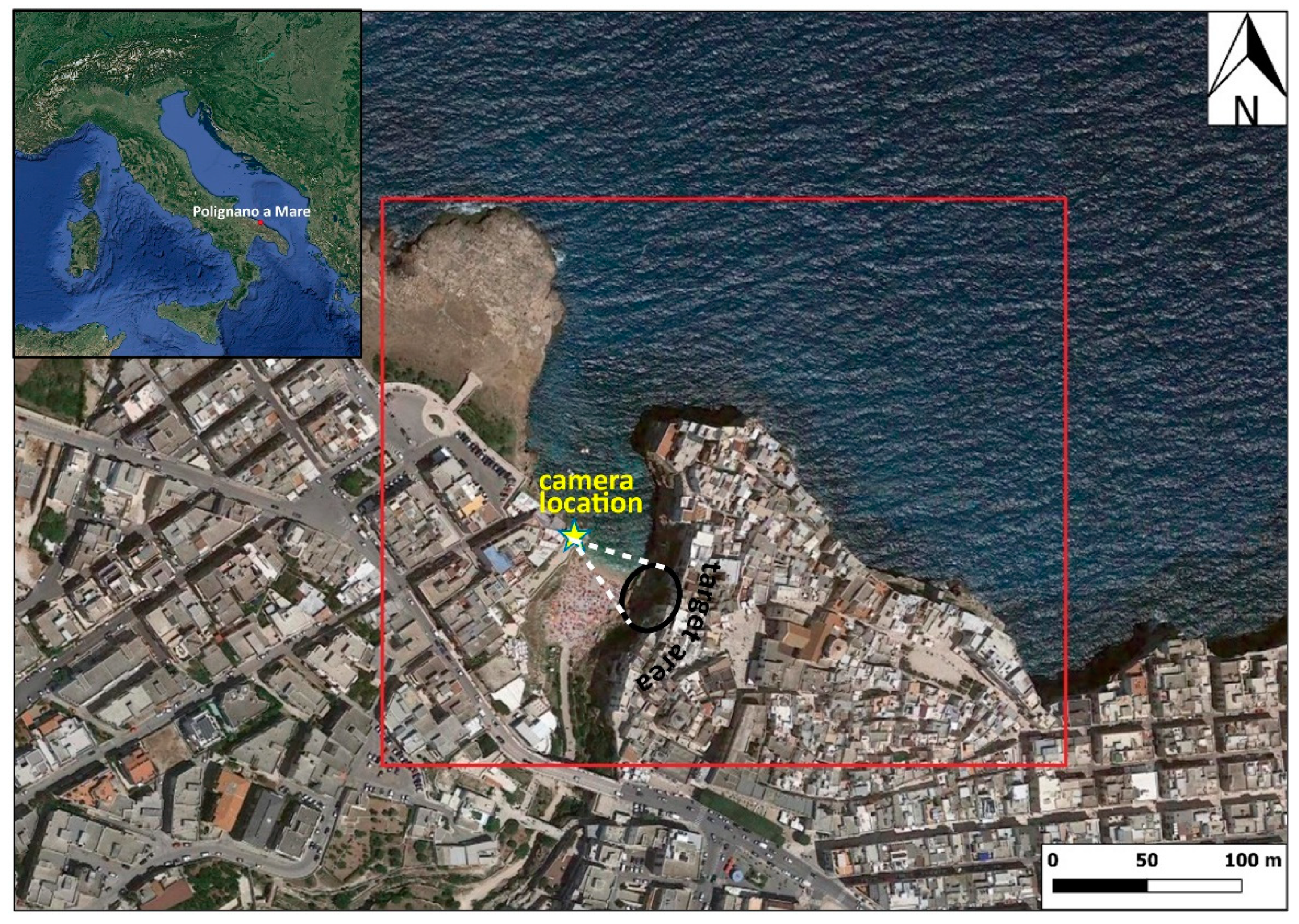
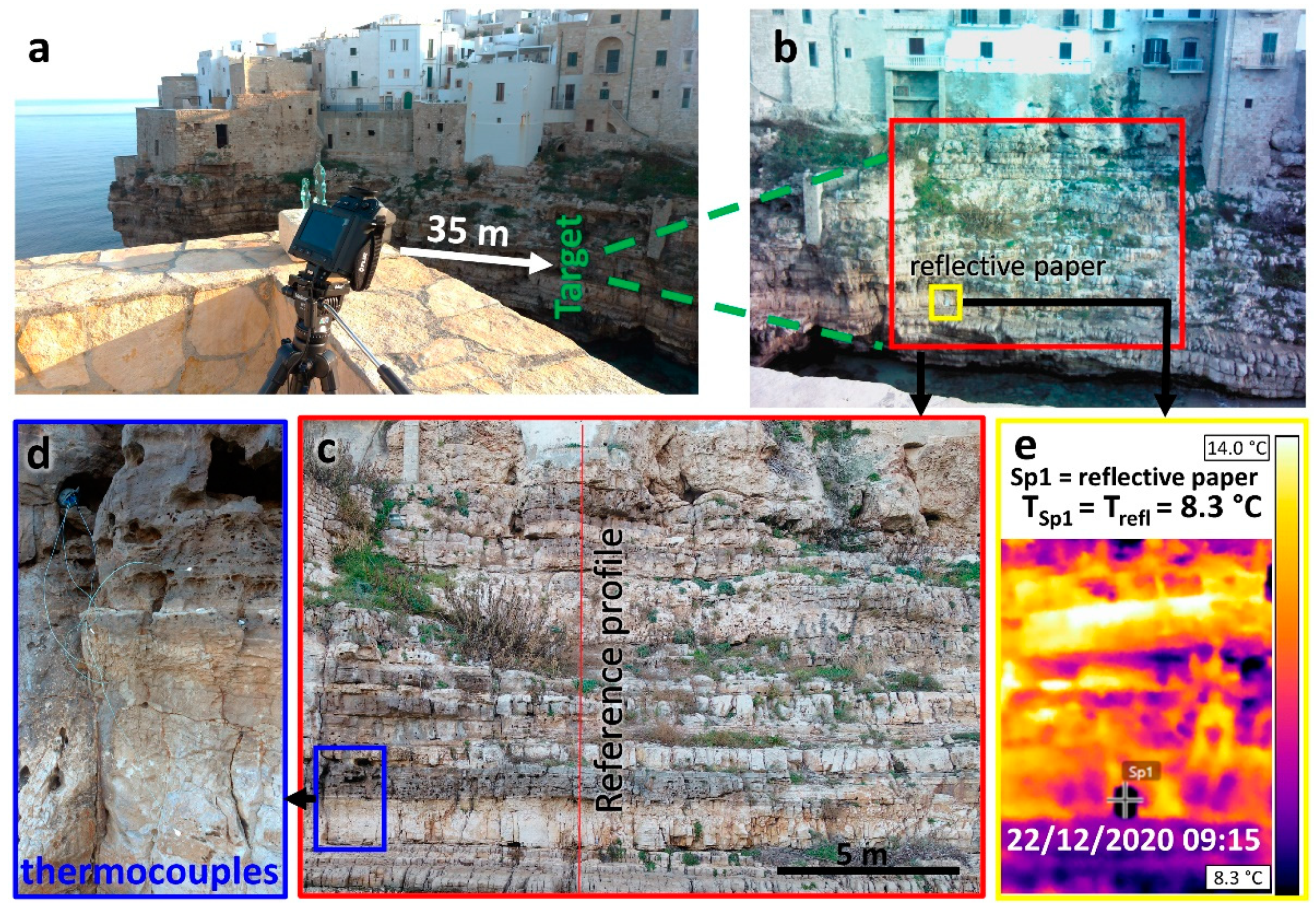
2.1. Case Study: Polignano a Mare (Southern Italy)

The study area is a 20-m high rock cliff facing the Adriatic Sea at the Lama Monachile site, a high-impact tourist destination at Polignano a Mare (southern Italy) (Figure 2). From a geologic standpoint, the site is constituted by a 3-km-thick Cretaceous bedrock, related to a wide carbonate platform, discontinuously overlain by transgressive quaternary deposits associated with shallow and agitated marine waters [40,41]. Morphology of the area is represented by a series of marine terraces parallel to the current coastline, which are the result of the superimposition of the regional uplift of Apulia started during the Lower Pleistocene and of glacio-eustatic sea level changes [42]. Lama Monachile is part of the network of karst valleys which crosses the marine terraces until reaching the Adriatic Sea, and takes its name from local terms describing the main types of karst incisions in Apulia [43,44]. In detail, lame are generally dry and slightly incised valleys with a flat bottom, in which the water flows during exceptional rainfall events, often originating flash floods in the karst environment, with severe negative effects [43,45,46,47,48].
Two geologic units crop out along the sides of Lama Monachile: limestones and dolostones belonging to the Calcare di Bari Fm. (Valanginian–late Cenomanian) and bio-calcarenites belonging to the Calcarenite di Gravina Fm. (upper Pliocene–early Pleistocene). Petrographic examination with transmitted light was performed on thin sections of representative samples, using optical polarizing microscopy. The Calcare di Bari Fm., which is formed by sub-horizontal thin to thick bedded layers (0.05–1 m), for a total thickness of 15 m, is constituted by two main lithofacies, whitish-greyish micritic limestones and grey-brown dolostones, alternating in the carbonate succession. The Calcarenite di Gravina Fm. overlies the Cretaceous bedrock through an angular erosional unconformity and reaches a total thickness of about 8 m in the study site, although the upper boundary is not well visible because of the buildings located at the top of the cliff. It is made up of poorly cemented, yellowish-greyish coarse to medium-grained calcarenites.
For both formations, dry density, saturated density, porosity, water absorption and degree of saturation were defined according to standard procedures [49,50] (Table 1). The Calcare di Bari Fm. has mean porosity values of approximately 9% and 4% for the micritic and dolomitic facies, respectively. The water absorption is 1–5% for the micritic facies and 0–2% for the dolomitic facies, while the degree of saturation varies in the range 36–100% and 50–90% for the micritic and dolomitic facies, respectively. The Calcarenite di Gravina samples are characterized by higher porosity (41%) and water absorption (18–30%). A degree of saturation of about 100% indicates that the pores in the rock particle are usually interconnected and continuous (high open primary porosity), in agreement with tests carried out on the same unit, in different Apulian sites [51,52]. By contrast, the Calcare di Bari Formation is characterized by isolated voids (secondary porosity), as demonstrated by the lower degree of saturation.
From a geostructural point of view, the Calcare di Bari Fm at Polignano a Mare is characterized by sub-horizontal bedding surfaces (S0) and two orthogonal subvertical joint sets striking NNE-SSW (J1) and ESE-WNW (J2), respectively (Figure 3a). Slight variation of the attitude of the discontinuities are locally determined by folds interpreted as the effects of transtentional and transpressional deformations [53]. The geostructural and geomechanical setting of the study site, determined by means of conventional geostructural and geomechanical surveys [54] and point cloud inspection, is summarized in Table 2. The mean discontinuity persistence was estimated according to the geometric relationships between the discontinuity traces and specific sampling windows, following the method proposed in [55]. The discontinuity surfaces are hardly recognizable in the calcarenite unit, which shows a massive structure (Figure 3b).
The rock mass is affected by heavy physical and chemical weathering, the effects of which are visible in the form of voids and cavities caused by karst processes, salt crystallization, wetting and drying cycles and biological activity, all factors potentially predisposing to detachment of rocks [56,57].
Despite the presence of subvertical rock walls, bushes and shrubs of the Mediterranean vegetation are diffuse over the rock mass (Figure 3b) and tend to grow with their root systems inside the fractures and voids, thus favoring aperture of the discontinuities. In addition, human works, such as terraces, excavation of artificial cavities and buildings partially carved, especially in the porous and soft calcarenites, modified the overall morphology, locally contributing to reduction of the strength properties. As a result, the structure of the rock mass and the surface conditions of the discontinuities are laterally and vertically variable. Based on these observations, a geological strength index [58,59,60] varying between 43 and 60 according to the local conditions was assigned to the rock mass at the Lama Monachile site. In detail, the GSI values of the limestone units were determined considering type “B” (thin to medium-bedded) and type “D” (blocky) structures and good–fair conditions of the discontinuities, on the basis of field and photograph inspection [59]. Regarding the calcarenite unit, a lower average GSI (43) was assigned to take into account the weathered surfaces.
The geomorphologic evolution of the cliff is represented by cliff recession through sporadic and localized instabilities, such as slides, topples, rockfalls and sea cave failures, mainly due to direct wave action on the Cretaceous limestone, and to strength decay of the calcarenite lithofacies at places enhanced by uncontrolled urbanization.
Although no landslides have been reported so far, it is evident that episodic failures, probably triggered by violent storms, even if involving small volumes, represent a serious risk for the community, considering the high frequency of tourists, both the historical center of Polignano a Mare, at the top of the cliff, and at the seaside at its toe during the summer season.

2.2. UAV and IRT Surveys

UAV surveys were carried out on the study site to support the interpretation of the IRT data taking advantage of the high-resolution photos and point cloud, to check if the thermal anomalies were related to the rock mass properties or to disturbance elements. The surveys were performed by means of a quadcopter platform DJI Inspire 2 equipped with a 20.8 megapixels (5280 × 3956 pixels) resolution camera and an integrated Global Navigation Satellite System (GNSS). Sixty-eight frontal photos were taken at 9 m from the rock wall, with side and frontal overlap of 85 and 75%, respectively. The Structure from Motion technique [61,62,63] was performed using Agisoft Metashape Professional software [64] (Agisoft LLC, St. Petersburg, Russia) and following the built-in workflow:
  • Photo inspection, importation and conversion of the coordinates into WGS84/33 N metric coordinate system.
  • High-accuracy camera alignment by means of sparse bundle adjustment algorithm [65].
  • High-quality depth maps calculation, generation of the dense point cloud (about 51 million points) and direct segmentation to remove unwanted objects.
In a second phase, the dense point cloud was aligned on a TLS point cloud previously georeferenced using a Stonex SIII Differential Global Positioning System (Stonex SRL, Monza, Italy). This step was necessary because of the impossibility to install enough ground control points during the UAV survey to correctly georeference the point cloud and avoid doming deformations [66,67,68,69]. The point clouds were split at couples in more sub-point clouds and independently aligned using the Iterative Closest Points (ICP) algorithm [70] until reaching a final root mean square Error of 43 mm. The final point cloud of the area addressed to the IRT surveys is constituted by about 16 million points and a surface density of 13,391 points/m2, corresponding to a mean point spacing of 9 mm (Figure 4).
Thermal data were acquired on the study site for 24 h starting from 21 December 2020 at 17:45 Central European Time (CET) using a FLIR T-660 thermal imager (Teledyne FLIR LLC, Wilsonville, Oregon, USA) mounted on a fixed tripod to ensure immobility of the camera. The FLIR T-660 camera has 5 MP built-in RGB camera and manufacturer-specified temperature measuring range of −40–+150 °C, measurement accuracy of ±1% of T °C, infrared spectral range of 7.5–14.0 μm, image resolution of 640 × 480 pixels, field of view (FOV) 25° × 19°, and focal length of 25 mm. The thermal sensitivity or noise equivalent temperature difference (NETD) is the apparent temperature difference between an object and its environment producing a signal equal to the noise of the system [71]. In other words, the NETD is the smallest temperature difference that can be detected by the thermal camera, whose value is less than 0.02 °C at 30 °C for the FLIR T-660. Seventy-three thermal images (thermograms) were acquired with a regular time-interval of 20 min. In addition, three type-K thermocouple sensors were positioned on three different lithofacies to compare and validate the surface temperatures recorded by the thermal camera. To avoid direct solar radiation on the sensors, the thermocouples were installed inside small cavities (dissolution voids deep up to 1–2 cm) of the rock wall (Figure 5d). The recorded data are reported in the supplementary materials (Table S1).
To correct the apparent temperatures and derive values close to the real ones, all factors that influence the results were recorded. Air temperature and relative humidity were measured before each thermal acquisition by means of a pocketsize digital thermohydrometer (Temperature measurement range= −25 ± 180 °C, humidity measurement range = 0–100%). A 35-m distance between the IRT camera and the target area was measured from point clouds obtained by means of Terrestrial Laser Scanning and Structure from Motion techniques. An emissivity coefficient equal to 0.92 was assumed from reference tables [3,72]. The reflector method [3,72,73] was used to measure the reflected temperature by placing an aluminium foil-covered cardboard at the base of the cliff (Figure 5b). Since the aluminium foil is an almost ideal reflector (emissivity = 0.05), the temperature measured on it (Figure 5e) corresponds to the ambient thermal radiations reflected by the reflector itself.

2.3. IRT Data Processing and Correlation with UAV Data

After the acquisition phase, the thermograms were processed using the FLIR Tools software [74]. In detail, the object emissivity, air temperature, relative humidity, reflected temperature and distance from the cliff were entered as input in the software, which automatically calculated the real temperatures by subtracting the radiation reflected from the ambient sources and emitted from the atmosphere to the total radiation received by the thermal imager. Successively, the range of the colour scale was adjusted for each thermogram to better detect cold and hot thermal anomalies.
The surface temperatures were extracted from all thermograms along a vertical profile positioned in a low-disturbed area (to avoid vegetation and anthropogenic elements) by means of a specifically compiled algorithm. After identifying the most appropriate profile, the developed algorithm automatically extracted, in all the thermograms, the temperature of the pixels crossed by the traced line. The data were processed in a spreadsheet to determine and plot the recorded temperatures, minimum, maximum, range, mean, median and standard deviation values for each pixel along the profile. Surface temperatures on the same vertical profile were plotted in a temperature-pixel frame to obtain the time-series with a 4 h sampling interval. In addition, a topographic profile was extracted from the point cloud along the same section to identify potential thermal anomalies caused by the topography of the rock face. The geological strength index (GSI) [58,59,60] and fracture frequency (i.e., number of fractures per unit length) for each layer were determined by means of measurements and qualitative observations on the point cloud and on the high-resolution photos acquired by the UAV system. Specifically, the GSI was estimated by defining the rock mass structure and the discontinuity conditions (i.e., roughness and weathering) for each layer, while the fracture frequency was calculated through linear scanlines, perpendicular to the main discontinuity sets, both in the field and from high-resolution georeferenced point clouds.
Finally, the plots were aligned to identify correlations among the surface temperatures and topography, lithology and degree of fracturing of the layers.

3. Results and Discussion

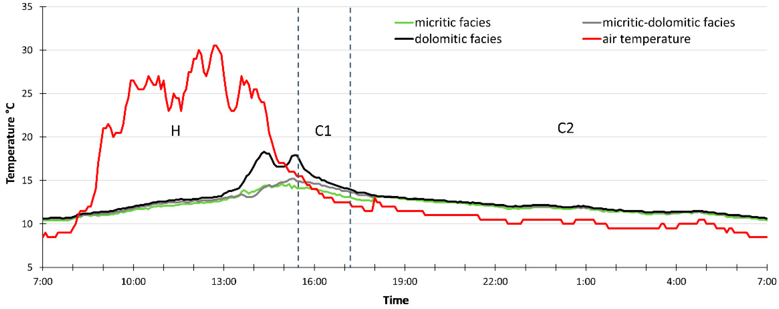
3.1. Environmental Conditions and Rock Temperature Curves

The use of the pocket-size thermo-hydrometer allowed the definition of the typical daily thermal cycles of sunny days in winter at Lama Monachile site, as well as the rock mass thermal response (Figure 6). In detail, the air temperature is in the range of 8.5–30.5 °C, with a maximum daily thermal excursion of 22 °C. The highest and lowest temperatures were recorded at midday and early morning, respectively. The relative humidity was in the range 39–96%, with a maximum variation of 57% (Figure 6). The rock mass is subjected to heat transfer determined by conduction, air convection and radiation processes [75]. The temperatures of the three lithofacies, directly measured by means of K-type thermocouple sensors in areas not affected by direct solar radiation, follow the air temperature curve, although with delay due to the natural low diffusivity of rocks (Figure 6). The heating phase (phase H in Figure 6) starts at dawn (7:12 CET): the rock mass heats up by direct solar radiation until reaching the peak temperature at about 15:30 CET. Later on, a first fast cooling phase (C1) is determined by the progressive shadowing of the cliff until the sunset (at 16:26 CET), followed by a slower nocturnal cooling phase (C2). With regards to the thermal behavior of the lithofacies cropping out, they show very similar temperature curves, especially for the micritic and micritic-dolomitic facies. The major difference was detected for the dolomitic facies, darker in color and characterized by a major number of voids, during the peak solar radiation hours (13:30–15:30 CET), when it reached a temperature 4 °C higher with respect to the other facies. The analyzed curves show that the heating phase is shorter than the cooling phase and is related to a fast rise of the rock temperature because of direct solar radiation. These outcomes are in agreement with the results of rock temperature direct (thermocouples) and indirect (IRT) measurements carried out in the Mediterranean area [18].

3.2. Time Series of Air-Rock Temperature and Correlations with Rock Mass Properties

The alignment of the temperature profiles along the reference section with those of the rock mass properties (e.g., topography, lithology, GSI, and fracture frequency) allowed the detection of some correlations (Figure 7). The disturbance elements such as vegetation and man-made structures (e.g., walls), which were detected as warm thermal anomalies in the thermograms acquired during the heating phase (Figure 8c), were removed from the temperature profiles. It must be remarked that, due to the high horizontal and vertical heterogeneity of the rock mass properties in terms of color, porosity (at the centimetric scale) and jointing degree, very close peaks characterized the temperature profiles, making the correlation phase quite complex. In addition, because of the large-scale irregularities and of the different local orientation of the slope sectors, the rock mass was not uniformly heated during the daytime. For this reason, the extracted temperature profiles along the reference section, which appeared unclear, were further processed to distinguish the thermal response of the target during the cooling and the heating phases. It is specified that the clearest correlations were obtained by analyzing the temperature profiles during the cooling phase (time range between 17:35 of 21 December 2020 and 6:55 of 22 December 2020, Figure 7), to avoid the effects of sun radiation. The correlations between the surface temperature profiles and the rock mass properties during the heating phase (time range between 6:55 and15:35 of 22 December 2020) are reported in the Supplementary Materials (Figure S1). The mentioned properties contribute together, in different proportions along the reference profile, to the definition of the rock mass thermal response. The prevalence of one property over the others was marked along the plots illustrated in Figure 7 (cooling phase) and validated by comparing the 2-D thermograms:
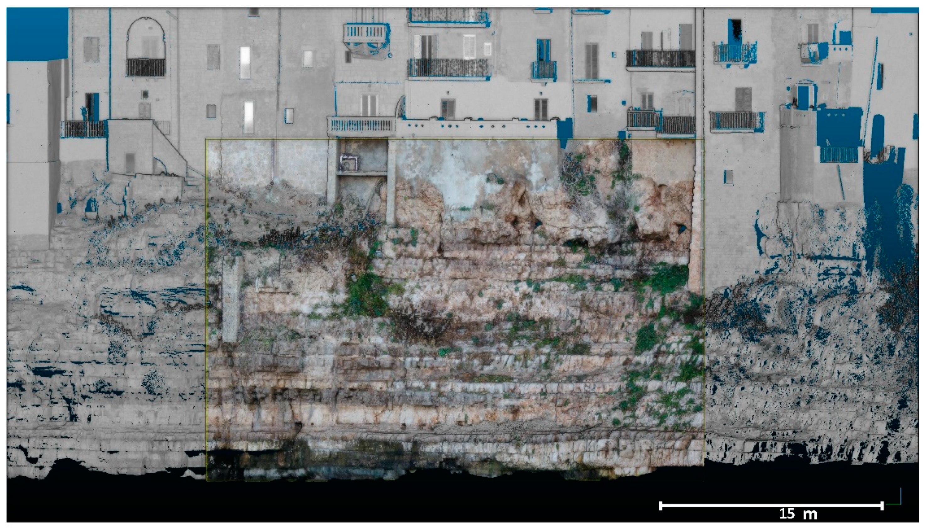
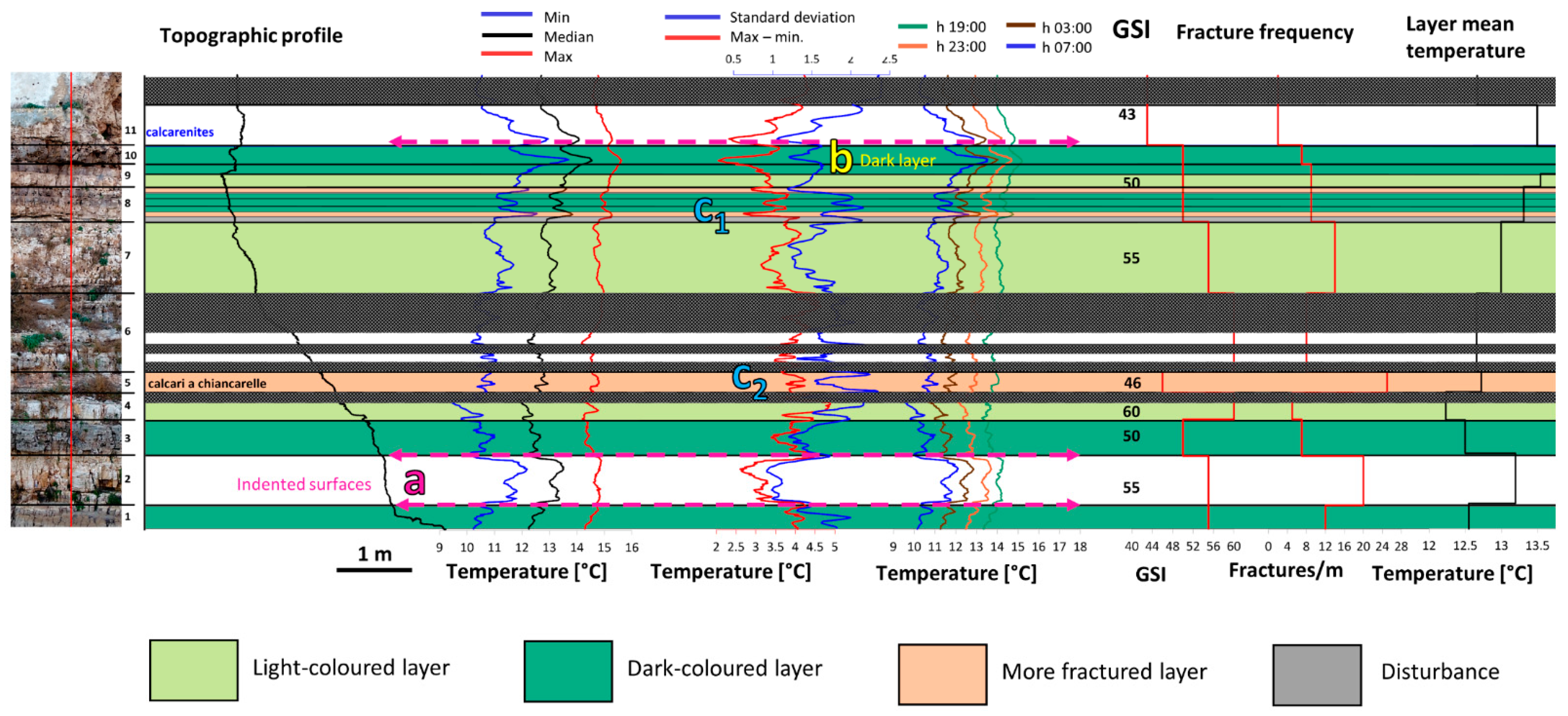
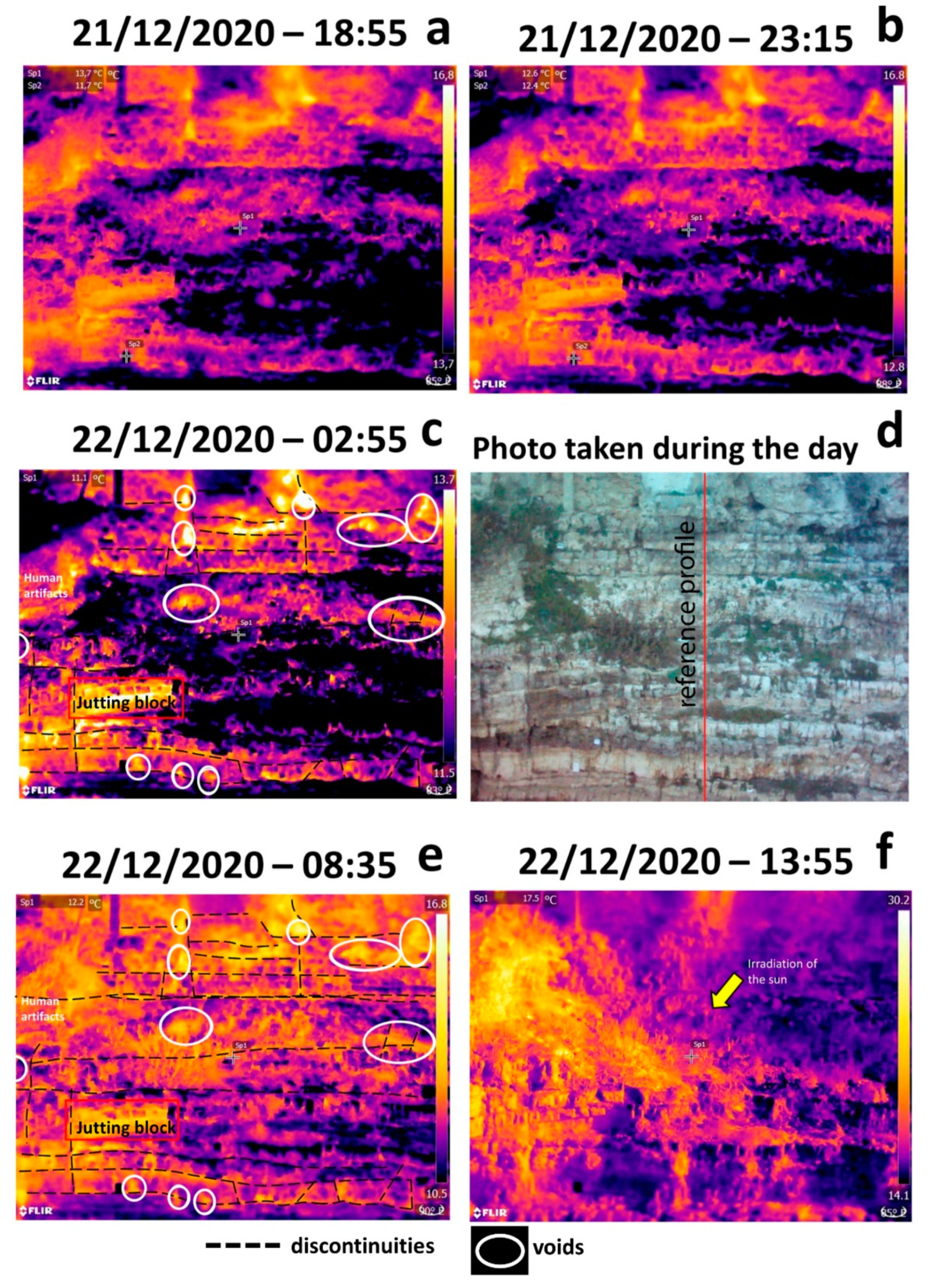
  • Correlation temperature-topography: lower temperatures (minimum, maximum, median, mean temperature per layer), larger standard deviations and larger difference values were detected along indented surfaces on the reference section like tight bedding planes, which were shadowed also during the daytime, and in correspondence of jutting blocks (Figure 7, Figure S1—marker “a”). On the contrary, higher temperatures, lower standard deviations and lower differences were found for the open discontinuities and the hollow sectors below the jutting blocks, in which the warm air was preserved. However, a jutting block (rectangle marker in Figure 8a and Figure 9c) was identified in the form of positive thermal anomaly during the nighttime. This discrepancy is probably related to the different attitude of the identified rock block that, being oriented parallel to the direction of the solar radiation, gained more heat during the daytime with respect to the other sectors of the rock mass.
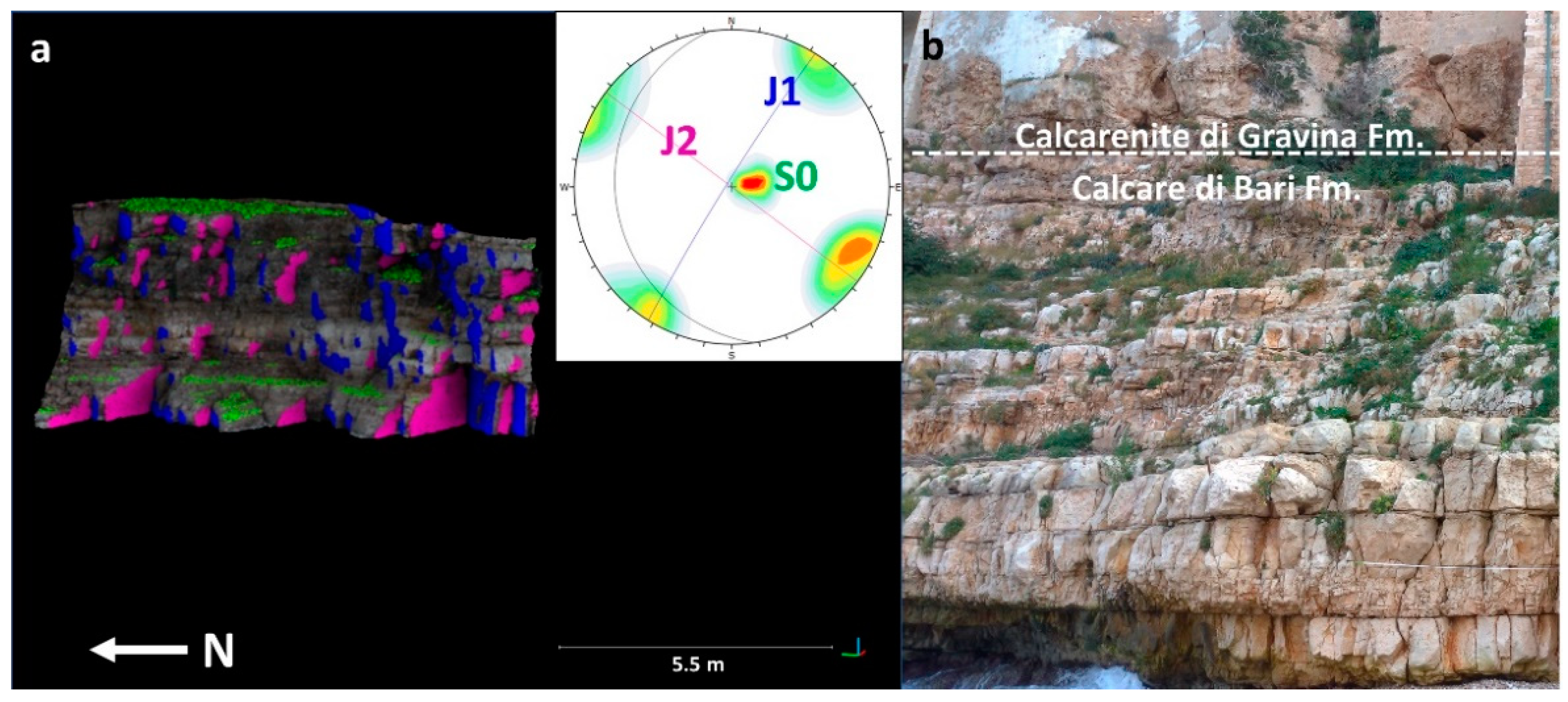
  • Correlation temperature-rock color: darker levels corresponding to the dolomitic facies are characterized by higher temperatures (minimum, maximum, median, mean temperature per layer) and lower values of the standard deviation and difference, related to a more constant distribution of the temperature during the day (e.g., Figure 7, Figure S1—marker “b”, Figure 8b).
  • Correlation temperature-jointing degree/GSI: higher temperature (minimum, maximum, median, mean temperature per layer) values were detected on the highly jointed layers (number of discontinuities/m and karst voids), characterized by lower GSI values (e.g., Figure 8a). However, the interpretation of the standard deviation and difference curves is uncertain: in some cases, they show negative peaks (Figure 7, marker c1 inside orange layer), while in others they show oscillating peaks (Figure 7, Figure S1—marker “c” inside orange layer). A possible explanation could be related to the discontinuity aperture: the layers represented by the marker c1 are formed by close joints, while that marked by c2 corresponds to a very fine laminated layer, with centimetric discontinuity apertures (Calcari a Chiancarelle). Moreover, the vegetation grown in the voids of the Calcari a Chiancarelle unit may have caused disturbances, too. As a matter of fact, the vegetation disturbed the thermograms acquired during the daytime and the nighttime, respectively, in the form of warm and cold thermal anomalies (Figure 8c).
The direct proportionality between the air-rock temperature and the fracturing degree of rock masses, observed through the correlations along the reference profile, is in accordance with the results proposed in the literature based on the analysis of thermograms [19,21,28,38].

3.3. Detection of Discontinuities in Thermal Images

3.3.1. Cooling Phase

The discontinuities, voids and hollow zones are visible in the thermograms acquired during the evening in the form of warmer anomalies (Figure 9a,b). As a matter of fact, while the intact rock gets colder during the cooling phase, warmer air is preserved in the discontinuity system [17]. The best moment to detect the geostructural features is late at night, when neither solar radiation or artificial lights disturb the acquisition (Figure 9c). This is consistent with data reported in [17,18,20,21,26,28], but a discrepancy was detected with regards to the thermal behavior of jutting blocks. The authors of [17,26] detected jutting blocks in the form of negative thermal anomalies in thermal images acquired during the night because of the higher exposure to ventilation. However, a jutting block of the study site was characterized by higher temperatures in all the thermograms (red rectangle in Figure 9). A possible explanation for this discrepancy is that the described block was more exposed to the solar radiation during the day because of its different attitude (SW, parallel to the direction of the sunrays during the peak hours) with respect to the overall aspect of the target area (NS). It is remarked that the discontinuities belonging to the bedding (S0) detected in the thermal outputs are clearer than those of the sub-vertical joint sets (J1, J2) because of the larger persistence driving a greater heat flow [25].

3.3.2. Heating Phase

In the early morning, the fractured and voided levels are heated by the solar radiation more quickly than the intact rock, which has a low thermal diffusivity. Thus, these structures are still visible in the form of positive thermal anomalies, but their contours are not well defined throughout the thermal image (Figure 9e). An interesting result of the IRT acquisition at early morning is that the calcarenite unit, which is in contact with the limestone unit, is not easy to define in the field and on high-resolution photos because of anthropogenic disturbances and weathered material, can be easily defined in the thermograms. This is due to the higher porosity and a high connectivity of the pore system, which allows the lithofacies to get warmer with respect to the other rock materials. Conversely, the Calcare di Bari Fm. showed a larger thermal inertia, as the warm air difficultly circulated in the pore system made up of isolated pores. However, moderately-intensely jointed layers in the limestone unit have temperatures comparable with those of the Calcarenite di Gravina Fm because of the warm air circulating inside the open fractures, which are represented by warm thermal anomalies, in agreement with the literature [12,17,21,24,26,31,38]. By analyzing the thermograms of the two formations of the study site, a discrepancy was found with respect to this aspect. As a matter of fact, the calcarenite unit generally shows higher temperatures with respect to the less porous limestone units, also during the nighttime (Figure 9a–c), implicating a lower cooling rate. A possible explanation is that the Calcare di Bari Fm., even if less porous, gets colder than the Calcarenite di Gravina Fm. because the heat is released through the discontinuity systems.
Later on, their identification of jointed and voided levels gets more uncertain because the vegetation, directly heated by the Sun, becomes much warmer and disturbs the thermal images. In addition, areas of the rock mass are differently illuminated depending on the daily solar path, until sunrise. Consequently, protruding sectors of the slope facing the direction of the solar radiation gain more heat and project their shadows on the indented and inner parts, which are represented by lower temperatures in the thermograms. These outcomes are in agreement with the results reported in [17,18,21,26,32]. For instance, Figure 9f illustrates that at 13:55 the sector of the rock mass with slightly different aspect (dipping SW) are warmer compared to the other zones as an effect of the solar radiation. In this case, it is not possible to detect discontinuities in the form of positive anomalies. This is consistent with data reported in the literature [17,21,26]. When the cooling phase is reached, the detection of discontinuities is again facilitated.

4. Main Outcomes and Conclusions

With this research, we tested the infrared thermography technique in a coastal area characterized by a humid mesothermal climate with mild winters and anthropogenic disturbances. The rock mass of the study area is made up of vertical and lateral hetereogeneous facies, characterized by different fabric, fracturing conditions, weathering and karst features. The aim of this study was to assess whether IRT technique in such a complex setting could be of support to the geomechanical characterization of rock masses and if it could provide additional information with respect to other remote sensing technologies, like laser scanners and drones.
By analyzing the rock temperatures, we found out that, with a daily thermal excursion of more than 20 °C, the lithofacies reached values of temperature differences up to 4–8 °C. In addition, as outlined in [18], it was observed that the heating phase is faster than the cooling phase (Figure 6) and that it is caused by short and intense solar radiation.
Detailed information on topography, lithology and fracturing conditions can be collected by aligning longitudinal profiles extracted from the thermograms, topographic profiles and high-resolution photos of the investigated area.
In addition, despite the low emissivity of the rock mass, the effect of solar radiation at the rock-air interface allowed the detection of geostructural information from the thermal images at a detailed scale. As a matter of fact, discontinuities, such as joints and bedding planes, karst voids and more fractured layers, were identified as positive thermal anomalies in the thermograms acquired at night-time, since they preserve the heat absorbed during the day.
With regard to the optimal time to acquire the IRT images, we realized that the night time represents the best conditions, since the detection of discontinuities and voids in the form of warm thermal anomalies is not affected by disturbances produced by vegetation, diurnal human activities and parasite radiations produced by the natural lights, in agreement with [17,18,20,21,25,26,28]. Conversely, thermograms obtained during the peak solar radiation do not allow the identification of weaker zones because the different illumination conditions give information only on the attitude of the sectors of the rock mass. For this reason, IRT surveys aimed at the detection of fractured and voided zones are not recommended when the angle of incidence of the sunrays is high. However, some IRT applications took advantage of the direct solar radiation to explore the three-dimensionality of rock slopes, to detect protruding or recessed blocks [17] and to identify discontinuities facing the sun direction as low thermal anomalies [25].
Concerning the limitations of IRT techniques, the logistics and complexity of the examined area represented the main issue. In detail, considering the high lateral and vertical heterogeneity of the lithofacies, as well as the presence of thin bedded and intensely jointed layers, success of IRT monitoring can be achieved only by means of high-resolution thermal images. In other words, if the survey is aimed at identifying more fractured zones or laminated levels, the pixel size must be smaller than the fracture spacing or the layer thickness. Nevertheless, the resolution of the thermograms is related to the distance between the IRT camera and the target area, which is often constrained to morphology conditions [25,37]. The issues related to the low-detailed thermal outputs can be solved by using IRT sensors with higher resolution. In addition, time-series plotted to find correlations between the surface rock temperatures and the rock mass properties along a longitudinal profile are sensitive to the position of the profile itself: when the peaks of the temperature-pixel curves are very close to each other (i.e., succession of heterogeneous facies), a bad alignment of the profiles extracted at different times may affect the results. It is thus recommended to ensure immobility of the thermal imager during the acquisition.
Furthermore, the interpretation of thermograms acquired in complex environments can be challenging because the resolution of the RGB photos taken by the thermal camera is not always sufficient to examine small-sized thermal anomalies. In this case, UAV techniques might be of paramount importance to zoom on the anomaly, locate the thermogram in a broader area and detect potential correlations with other geostructural features.
With this study we outlined how infrared thermography can be of support for geostructural analyses in rock masses, even in areas with mild climate, disturbance elements and characterized by heterogeneous successions made up of lithofacies with similar emissivity and not always clear contacts, due to different degrees of degradation even at a large scale and with the support of high-resolution photos.
The integration of IRT results with field observations and other remote sensing technologies might be fundamental for the identification of overhanging sectors of rock masses defined by persistent and open joints, subjected to major thermal stresses and susceptible to failure over time.

Supplementary Materials

The following supporting information can be downloaded at: https://0-www-mdpi-com.brum.beds.ac.uk/article/10.3390/geosciences12030116/s1, Table S1: Calibration parameters measured during the acquisition process (21–22 December 2020) for the correction of the apparent temperatures. The ambient air temperature and relative humidity were measured by means of a pocket-size digital thermo-hydrometer, and the reflected temperature was calculated using a reflective target at the base of the cliff to calculate the real temperatures [3,72,73]. Figure S1: Composite plot illustrating how the surface rock temperatures detected from the IRT camera along the section during the heating phase were determined by the interaction of different factors. It is remarked that the correlations between the air-rock surface temperatures and the rock mass properties are less clear than those of the cooling phase because of the effects of sun radiation and irregular surfaces. (a) Lower temperatures and higher temperature standard deviation and differences were identified in correspondence of the indented surfaces (i.e., layer interfaces and tight discontinuities). Conversely, open discontinuities and karst voids are represented by higher temperatures, as the warm air circulates within the discontinuity system; (b) darker levels (dolomitic facies, in dark green) show higher temperatures and lower standard deviation and differences with respect to the lighter levels (micritic limestones, in light green); (c1, c2) higher temperatures are associated with levels with a higher fracture frequency and/or more dissolution voids (low GSI). The standard deviation and difference values in correspondence of moderately jointed layers were generally detected in the form of negative peaks.

Author Contributions

Conceptualization, L.L. and G.F.A.; methodology, L.L., M.J. and M.-H.D.; investigation, L.L., G.F.A. and M.P.; writing—original draft preparation, L.L.; writing—review and editing, L.L., G.F.A., M.-H.D., M.J. and M.P.; visualization, M.-H.D.; validation and supervision, M.J. and M.P. All authors have read and agreed to the published version of the manuscript.

Funding

This research received no external funding.

Acknowledgments

We thank the anonymous reviewers for their support and suggestions in the reviewing phase of this paper.

Conflicts of Interest

The authors declare no conflict of interest.

References

  1. Wolfe, W.L.; Zissis, G.J. The Infrared Handbook; General Dynamics: Reston, VA, USA, 1985. [Google Scholar]
  2. Dewitt, D.P.; Nutter, G.D. Theory and Practice of Radiation Thermometry; John Wiley & Sons: Hoboken, NJ, USA, 1988. [Google Scholar]
  3. FLIR. User’s Manual FLIR T6xx Series. 2014. Available online: https://flir.custhelp.com/app/account/fl_download_manuals (accessed on 11 December 2021).
  4. Shannon, H.; Sigda, J.; van Dam, R.; Hendrickx, J.; Mclemore, V. Thermal camera imaging of rock piles at the Questa Molybdenum Mine, Questa, New Mexico. In Proceedings of the 22nd American Society of Mining and Reclamation Annual National Conference, Breckenridge, CO, USA, 18–25 June 2005. [Google Scholar]
  5. Prendes-Gero, M.-B.; Suárez-Domínguez, F.J.; González-Nicieza, C.; Álvarez-Fernández, M.I. Infrared thermography methodology applied to detect localized rockfalls in self-supporting underground mines. In Proceedings of the EUROCK 2013—The 2013 ISRM International Symposium—Rock Mechanics for Resources, Energy, and Environment, Wroclaw, Poland, 23–26 September 2013. [Google Scholar]
  6. Rees, W.G. Physical Principles of Remote Sensing; Cambridge University Press: Cambridge, UK, 2012. [Google Scholar]
  7. Mineo, S.; Pappalardo, G. Rock emissivity measurement for infrared thermography engineering geological applications. Appl. Sci. 2021, 11, 3773. [Google Scholar] [CrossRef]
  8. Mongillo, M.A.; Wood, C.P.; Mongillo, M.A.; Wood, C.P. Thermal infrared mapping of White Island volcano, New Zealand. JVGR 1995, 69, 59–71. [Google Scholar] [CrossRef]
  9. Moxham, R.M.; Crandell, D.R.; Marlatt, W. Thermal features at Mount Rainier, Washington, as revealed by infrared surveys. US Geol. Surv. Prof. Pap. 1965, 1326, 93–100. [Google Scholar]
  10. Frodella, W.; Fidolini, F.; Morelli, S.; Pazzi, V. Application of infrared thermography for landslide mapping: The Rotolon DSGDS case study. Rend. Online Soc. Geol. Ital. 2015, 35, 144–147. [Google Scholar] [CrossRef]
  11. Frodella, W.; Morelli, S.; Pazzi, V. InfraRed thermographic surveys for landslide mapping and characterization: The Rotolon DSGSD (Northern Italy) case study. Ital. J. Eng. Geol. Environ. 2017, 1, 77–84. [Google Scholar]
  12. Baroň, I.; Bečkovský, D.; Míča, L. Application of infrared thermography for mapping open fractures in deep-seated rockslides and unstable cliffs. Landslides 2012, 11, 15–27. [Google Scholar] [CrossRef]
  13. Pappalardo, G.; Mineo, S.; Angrisani, A.C.; di Martire, D.; Calcaterra, D. Combining field data with infrared thermography and DInSAR surveys to evaluate the activity of landslides: The case study of Randazzo Landslide (NE Sicily). Landslides 2018, 15, 2173–2193. [Google Scholar] [CrossRef]
  14. Guerin, A.; Jaboyedoff, M.; Collins, B.D.; Derron, M.-H.; Stock, G.M.; Matasci, B.; Boesiger, M.; Lefeuvre, C.; Podladchikov, Y.Y. Detection of rock bridges by infrared thermal imaging and modeling. Sci. Rep. 2019, 9, 1–19. [Google Scholar] [CrossRef] [Green Version]
  15. Rinker, J.N. Airborne infrared thermal detection of caves and crevasses. Photogramm. Eng. Remote Sens. 1975, 41, 1391–1400. [Google Scholar]
  16. Liu, S.; Xu, Z.; Wu, L.; Ma, B.; Liu, X. Infrared imaging detection of hidden danger in mine engineering. In Proceedings of the Progress in Electromagnetics Research Symposium, Suzhou, China, 12–16 September 2011. [Google Scholar]
  17. Mineo, S.; Calcaterra, D.; Zampelli, S.P.; Pappalardo, G. Application of infrared thermography for the survey of intensely jointed rock slopes. Rend. Online Soc. Geol. Ital. 2015, 35, 212–215. [Google Scholar] [CrossRef]
  18. Fiorucci, M.; Marmoni, G.M.; Martino, S.; Mazzanti, P. Thermal response of jointed rock masses inferred from infrared thermographic surveying (Acuto test-site, Italy). Sensors 2018, 7, 2221. [Google Scholar] [CrossRef] [PubMed] [Green Version]
  19. Squarzoni, C.; Galgaro, A.; Teza, G.; Acosta, C.A.T.; Pernito, M.A.; Bucceri, N. Terrestrial laser scanner and infrared thermography in rock fall prone slope analysis. Geophys. Res. Abstr. 2008, 10. 2008–09254. [Google Scholar]
  20. Teza, G.; Marcato, G.; Castelli, E.; Galgaro, A. IRTROCK: A MATLAB toolbox for contactless recognition of surface and shallow weakness of a rock cliff by infrared thermography. Comput. Geosci. 2012, 45, 109–118. [Google Scholar] [CrossRef]
  21. Pappalardo, G.; Mineo, S. Study of jointed and weathered rock slopes through the innovative approach of InfraRed thermography. Landslides Theory Pract. Model. 2019, 85–103. [Google Scholar]
  22. Frodella, W.; Gigli, G.; Morelli, S.; Lombardi, L.; Casagli, N. Landslide mapping and characterization through infrared thermography (IRT): Suggestions for a methodological approach from some case studies. Remote Sens. 2017, 9, 1281. [Google Scholar] [CrossRef] [Green Version]
  23. Adorno, V.; Barnobi, L.; la Rosa, F.; Leotta, A.; Paratore, M. Contributo della tecnologia laser scanner e termografia R nella caratterizzazione geomeccanica di un costone roccioso. In Proceedings of the Atti 13a Conferenza Nazionale ASITA, Bari, Italy, 1–4 December 2009. [Google Scholar]
  24. Gigli, G.; Frodella, W.; Garfagnoli, F.; Morelli, S.; Mugnai, F.; Menna, F.; Casagli, N. 3-D geomechanical rock mass characterization for the evaluation of rockslide susceptibility scenarios. Landslides 2013, 11, 131–140. [Google Scholar] [CrossRef]
  25. Frodella, W.; Morelli, S.; Gigli, G.; Casagli, N. Contribution of infrared thermography to the slope instability characterization. In Proceedings of the World Landslide Forum, Beijing, China, 2–6 June 2014; pp. 144–147. [Google Scholar]
  26. Pappalardo, G.; Mineo, S.; Zampelli, S.P.; Cubito, A.; Calcaterra, D. InfraRed Thermography proposed for the estimation of the cooling rate index in the remote survey of rock masses. Int. J. Rock Mech. Min. Sci. 2016, 83, 182–196. [Google Scholar] [CrossRef]
  27. Mineo, S.; Pappalardo, G.; Rapisarda, F.; Cubito, A.; di Maria, G. Integrated geostructural, seismic and infrared thermography surveys for the study of an unstable rock slope in the Peloritani Chain (NE Sicily). Eng. Geol. 2015, 195, 225–235. [Google Scholar] [CrossRef]
  28. Chicco, J.M.; Vacha, D.; Mandrone, G. Thermo-physical and geo-mechanical characterization of faulted carbonate rock masses (Valdieri, Italy). Remote Sens. 2019, 11, 179. [Google Scholar] [CrossRef] [Green Version]
  29. Wu, J.H.; Lin, H.M.; Lee, D.H.; Fang, S.C. Integrity assessment of rock mass behind the shotcreted slope using thermography. Eng. Geol. 2005, 80, 164–173. [Google Scholar] [CrossRef]
  30. Pappalardo, G.; Mineo, S.; Imposa, S.; Grassi, S.; Leotta, A.; la Rosa, F.; Salerno, D. A quick combined approach for the characterization of a cliff during a post-rockfall emergency. Landslides 2020, 17, 1063–1081. [Google Scholar] [CrossRef]
  31. Casagli, N.; Frodella, W.; Morelli, S.; Tofani, V.; Ciampalini, A.; Intrieri, E.; Raspini, F.; Rossi, G.; Tanteri, L.; Lu, P. Spaceborne, UAV and ground-based remote sensing techniques for landslide mapping, monitoring and early warning. Geoenviron. Disasters 2017, 4, 1–23. [Google Scholar] [CrossRef]
  32. Loche, M.; Scaringi, G.; Blahůt, J.; Melis, M.T.; Funedda, A.; da Pelo, S.; Erbì, I.; Deiana, G.; Meloni, M.A.; Cocco, F. An infrared thermography approach to evaluate the strength of a rock cliff. Remote Sens. 2021, 13, 1265. [Google Scholar] [CrossRef]
  33. Mineo, S.; Pappalardo, G. InfraRed thermography presented as an innovative and non-destructive solution to quantify rock porosity in laboratory. Int. J. Rock Mech. Min. Sci. 2019, 115, 99–110. [Google Scholar] [CrossRef]
  34. Deng, N.-F.; Qiao, L.; Li, Q.; Hao, J.-W.; Wu, S. A method to predict rock fracture with infrared thermography based on heat diffusion analysis. Geofluids 2021, 1–13. [Google Scholar] [CrossRef]
  35. Liu, Q.; Liu, Q.; Pan, Y.; Peng, X.; Deng, P.; Huang, K. Experimental study on rock indentation using infrared thermography and acoustic emission techniques. J. Geophys. Eng. 2018, 15, 1864–1877. [Google Scholar] [CrossRef] [Green Version]
  36. Junique, T.; Vazquez, P.; Thomachot-Schneider, C.; Hassoun, I.; Jean-Baptiste, M.; Géraud, Y. The use of infrared thermography on the measurement of microstructural changes of reservoir rocks induced by temperature. Appl. Sci. 2021, 11, 559. [Google Scholar] [CrossRef]
  37. Grechi, G.; Fiorucci, M.; Marmoni, G.M.; Martino, S. 3D thermal monitoring of jointed rock masses through infrared thermography and photogrammetry. Remote Sens. 2021, 13, 957. [Google Scholar] [CrossRef]
  38. Mineo, S.; Caliò, D.; Pappalardo, G. UAV-based photogrammetry and infrared thermography applied to rock mass survey for geomechanical purposes. Remote Sens. 2022, 14, 473. [Google Scholar] [CrossRef]
  39. Loiotine, L.; Andriani, G.F.; Jaboyedoff, M.; Parise, M.; Derron, M.-H. Comparison of remote sensing techniques for geostructural analysis and cliff monitoring in coastal areas of high tourist attraction: The case study of Polignano a Mare (Southern Italy). Remote Sens. 2021, 13, 5045. [Google Scholar] [CrossRef]
  40. Ricchetti, G.; Ciaranfi, N.; Luperto-Sinni, E.; Mongelli, F.; Pieri, P. Geodinamica ed evoluzione sedimentaria e tettonica dell’avampaese apulo. Mem. Soc. Geol. It. 1988, 41, 57–82. [Google Scholar]
  41. Tropeano, M.; Sabato, L. Response of Plio-Pleistocene mixed bioclastic-lithoclastic temperate-water carbonate systems to forced regressions: The Calcarenite di Gravina Formation, Puglia, SE Italy. Geol. Soc. Lond. 2000, 172, 217–243. [Google Scholar] [CrossRef]
  42. Ciaranfi, N.; Pieri, P.; Ricchetti, G. Note alla carta geologica delle Murge e del Salento (Puglia centromeridionale). Mem. Soc. Geol. Ital. 1988, 41, 449–460. [Google Scholar]
  43. Parise, M.; Federico, A.; delle Rose, M.; Sammarco, M. Karst terminology in Apulia (southern Italy). Acta Carsologica 2003, 32, 65–82. [Google Scholar] [CrossRef]
  44. Parise, M. Surface and subsurface karst geomorphology in the Murge (Apulia, southern Italy). Acta Carsologica 2011, 40, 79–93. [Google Scholar] [CrossRef]
  45. Parise, M. Hazards in karst. In Proceedings of the International Interdisciplinary Scientific Conference, Plitvice Lakes, Croatia, 23–26 September 2009; pp. 155–162. [Google Scholar]
  46. Bonacci, O.; Ljubenkov, I.; Roje-Bonacci, T. Karst flash floods: An example from the Dinaric Karst (Croatia). Nat. Hazards Earth Syst. Sci. 2006, 6, 195–203. [Google Scholar] [CrossRef] [Green Version]
  47. Gutiérrez, F.; Parise, M.; de Waele, J.; Jourde, H. A review on natural and human-induced geohazards and impacts in Karst. Earth-Sci. Rev. 2014, 138, 61–88. [Google Scholar] [CrossRef]
  48. Del Prete, S.; Iovine, G.; Parise, M.; Santo, A. Origin and distribution of different types of sinkholes in the plain areas of southern Italy. Geodin. Acta 2010, 23, 113–127. [Google Scholar] [CrossRef]
  49. Ulusay, R. (Ed.) The ISRM Suggested Methods for Rock Characterization, Testing and Monitoring: 2007–2014; Springer: Berlin/Heidelberg, Germany, 2015; ISBN 978-3-319-07712-3. [Google Scholar]
  50. ISRM. Suggested methods for determining the uniaxial compressive strength and deformability of rock materials. Int. J. Rock Mech. Min. Sci. Geomech. Abstr. 1979, 16, 135–140. [Google Scholar]
  51. Andriani, G.; Walsh, N. Fabric, porosity and water permeability of calcarenites from Apulia (SE Italy) used as building and ornamental stone. Bull. Eng. Geol. Environ. 2003, 62, 77–84. [Google Scholar] [CrossRef]
  52. Andriani, G.F.; Pastore, N.; Giasi, C.I.; Parise, M. Hydraulic properties of unsaturated calcarenites by means of a new integrated approach. J. Hydrol. 2021, 602, 126730. [Google Scholar] [CrossRef]
  53. Andriani, G.; Pellegrini, V. Qualitative assessment of the cliff instability susceptibility at a given scale with a new multidirectional method. Int. J. Geol. 2014, 8, 73–80. [Google Scholar]
  54. ISRM. Suggested methods for the quantitative description of discontinuities in rock masses. Int. J. Rock Mech. Min. Sci. Géoméch. Abstr. 1988, 20, 189–200. [Google Scholar]
  55. Pahl, P.J. Estimating the mean length of discontinuity traces. Int. J. Rock Mech. Min. Sci. Géoméch. Abstr. 1981, 18, 221–228. [Google Scholar] [CrossRef]
  56. Lollino, P.; Martimucci, V.; Parise, M. Geological survey and numerical modeling of the potential failure mechanisms of underground caves. Geosyst. Eng. 2013, 16, 100–112. [Google Scholar] [CrossRef]
  57. Parise, M.; Ravbar, N.N.; Živanović, V.; Mikszewski, A.; Kresic, N.; Mádl-Szőnyi, J.; Kukuric, N.; Kukurić, N. Hazards in Karst and managing water resources quality. In Karst Aquifers—Characterization and Engineering; Stevanovic, Z., Ed.; Professional Practice in Earth Sciences; Springer: Berlin/Heidelberg, Germany, 2015; pp. 601–687. [Google Scholar]
  58. Hoek, E.; Brown, E.T. The hoek-brown failure criterion and GSI—2018 edition. J. Rock Mech. Geotech. Eng. 2018, 11, 445–463. [Google Scholar] [CrossRef]
  59. Marinos, V. New proposed GSI classification charts for weak or complex rock masses. Bull. Geol. Soc. Greece 2017, 43, 1248. [Google Scholar] [CrossRef] [Green Version]
  60. Marinos, P.; Hoek, E. GSI—A geologically friendly tool for rock mass strength estimation. In Proceedings of the International Conference on Geotechnical and Geological Engineering (GeoEng2000), Melbourne, VIC, Australia, 19–24 November 2000; pp. 1422–1442. [Google Scholar]
  61. Carrivick, J.L.; Smith, M.W.; Quincey, D.J. Structure from Motion in the Geosciences; John Wiley & Sons: Hoboken, NJ, USA, 2016. [Google Scholar]
  62. Eltner, A.; Sofia, G. Structure from motion photogrammetric technique. In Developments in Earth Surface Processes; Elsevier: Amsterdam, The Netherlands, 2020; Volume 23, pp. 1–24. ISBN 9780444641779. [Google Scholar]
  63. Westoby, M.J.; Brasington, J.; Glasser, N.F.; Hambrey, M.J.; Reynolds, J.M. “Structure-from-motion” photogrammetry: A low-cost, effective tool for geoscience applications. Geomorphology 2012, 179, 300–314. [Google Scholar] [CrossRef] [Green Version]
  64. Agisoft LLC, Agisoft Metashape Professional Software, Version 1.6 2020, 160. St. Petersburg, Russia. Available online: https://www.agisoft.com/downloads/installer/ (accessed on 12 October 2021).
  65. Snavely, N.; Seitz, S.M.; Szeliski, R. Modeling the world from internet photo collections. Int. J. Comput. Vis. 2008, 80, 189–210. [Google Scholar] [CrossRef] [Green Version]
  66. Rosnell, T.; Honkavaara, E. Point cloud generation from aerial image data acquired by a quadrocopter type micro unmanned aerial vehicle and a digital still camera. Sensors 2012, 12, 453–480. [Google Scholar] [CrossRef] [Green Version]
  67. James, M.R.; Robson, S. Mitigating systematic error in topographic models derived from UAV and ground-based image networks. Earth Surf. Process. Landf. 2014, 39, 1413–1420. [Google Scholar] [CrossRef] [Green Version]
  68. Javernick, L.; Brasington, J.; Caruso, B. Modeling the topography of shallow braided rivers using structure-from-motion photogrammetry. Geomorphology 2014, 213, 166–182. [Google Scholar] [CrossRef]
  69. Ruggles, S.; Clark, J.; Franke, K.W.; Wolfe, D.; Reimschiissel, B.; Martin, R.A.; Okeson, T.J.; Hedengren, J.D. Comparison of SfM computer vision point clouds of a landslide derived from multiple small UAV platforms and sensors to a TLS-based model. J. Unmanned Veh. Syst. 2016, 4, 246–265. [Google Scholar] [CrossRef]
  70. Besl, P.J.; McKay, N.D. A method for registration of 3-D shapes. In Sensor Fusion IV: Control Paradigms and Data Structures; International Society for Optics and Photonics: Bellingham, WA, USA, 1992; Volume 1611, pp. 586–606. [Google Scholar]
  71. Gaussorgues, G. Infrared Thermography; Springer Science & Business Media: Berlin/Heidelberg, Germany, 1994. [Google Scholar]
  72. Hudson, R.D. Infrared System Engineering; Wiley: Hoboken, NJ, USA, 1969; Volume 1. [Google Scholar]
  73. Usamentiaga, R.; Venegas, P.; Guerediaga, J.; Vega, L.; Molleda, J.; Bulnes, F.G. Infrared thermography for temperature measurement and non-destructive testing. Sens. Switz. 2014, 14, 12305–12348. [Google Scholar] [CrossRef] [Green Version]
  74. FLIR Tools Thermal Analysis and Reporting (Desktop). Teledyne FLIR. Available online: https://www.flir.com/products/flir-tools/ (accessed on 6 July 2021).
  75. Robertson, E.C. Thermal Properties of Rocks; US Department of the Interior: Washington, DC, USA, 1988; pp. 88–441. [Google Scholar]
Figure 1. Schematic representation of the InfraRed spectrum (modified after [7]).
Geosciences 12 00116 g001
Figure 2. Location of the study area (base map retrieved from Google Satellite). The thermal imager is represented by the yellow marker.
Geosciences 12 00116 g002
Figure 3. Geostructural setting of the study site; (a) sub-vertical joint sets (J1, J2) and bedding surfaces (S0) detected in the Calcare di Bari Fm. by means of field surveys and UAV point cloud inspection; (b) details of the fracture network in the Calcare di Bari Fm. and of the massive structure of the Calcarenite di Gravina Fm.
Geosciences 12 00116 g003
Figure 4. Final high-resolution point cloud (RGB colors) of the study site obtained by means of UAV technique and aligned on a georeferenced TLS point cloud (in gray) to avoid doming deformations. The UAV point cloud has a surface density of 13391 points/m2, corresponding to a mean point spacing of 9 mm.
Geosciences 12 00116 g004
Figure 5. Setup of the IRT acquisition. (a) Location of the FLIR T-660 thermal camera and perspective view of the target; (b) frontal view of the target area and position of the reflective paper (yellow square); (c) zoom of the investigated area and scanline for the extraction of the thermal and lithologic profile; (d) location of the thermocouples for the temperature monitoring of the lithofacies; (e) example of measurement of the reflected temperature using the reflector method.
Geosciences 12 00116 g005
Figure 6. Air temperature and rock temperature directly measured on the outcropping lithofacies during the IRT monitoring by means of K-type thermocouples. H: fast heating phase, the rock materials reach the peak temperature at about 15:30; C1: first cooling phase, the progressive shadowing of the outcrop causes a drop of the rock temperatures; C2: a slower cooling phase occurs during the night.
Geosciences 12 00116 g006
Figure 7. Composite plot illustrating how the surface rock temperatures detected from the IRT camera along the section during the cooling phase were determined by the interaction of different factors. The areas covered by vegetation (in gray) were filtered out during the analysis. (a) Lower temperatures and higher temperature standard deviation and differences were identified in correspondence with the indented surfaces (i.e., layer interfaces and tight discontinuities) and jutting blocks; (b) darker levels (dolomitic facies, in dark green) show higher temperatures and lower standard deviation and differences with respect to the lighter levels (micritic limestones, in light green); (c1,c2) higher temperatures are associated to levels with a higher fracture frequency and/or more dissolution voids (low GSI). The standard deviation and difference values in correspondence of moderately jointed layers were generally detected in the form of negative peaks.
Geosciences 12 00116 g007
Figure 8. Correlation temperature-rock mass properties on the thermograms and RGB photos; (a) higher temperatures (yellow) detected on jutting blocks (white rectangle) and intensely jointed layers (white dotted line); (b) higher temperatures identified on darker levels (dolomitic facies); (c) disturbance produced by man-made structures (walls, white circle) and vegetation (black circle) especially during the daytime acquisitions.
Geosciences 12 00116 g008
Figure 9. Detection of discontinuities and voids in the thermal images acquired during the 24-h monitoring. (ac) Cooling phase: the discontinuities and voids were identified as warmer anomalies, in contrast with the intact rock which was colder; (d) RGB photo acquired by the thermal imager during the day; (e,f) heating phase: the discontinuities and voids gain more heat than the intact rock (low thermal diffusivity), but their contours are less defined. (e) The more porous calcarenite facies is identified in the form of warm thermal anomaly; (f) the discontinuities and voids cannot be detected because of the effects of direct solar radiation on the rock mass.
Geosciences 12 00116 g009
Table 1. Physical properties of the materials cropping out at the study site.
PropertyCalcarenite di GravinaCalcare di Bari
Micritic Facies
Calcare di Bari
Dolomitic Facies
MinMaxMeanMinMaxMeanMinMaxMean
Dry density (Mg/m3)1.481.721.602.442.522.472.472.722.62
Sat. density (Mg/m3)1.882.061.972.492.572.522.522.732.64
Porosity, n (%)36.1345.1640.756.8111.489.030.689.744.47
water absorption, wa (%)18.2929.6923.061.004.792.690.211.961.03
Degree of saturation, Sr %73.9199.7789.9836.0699.8470.9049.7489.6170.84
Table 2. Main geostructural and geomechanical parameters of the Calcare di Bari Fm.
DSTypeMean
Dip Direction
°
Mean
Dip
°
Weight %Spacing
(m)
Persistence
(m)
Aperture
(cm)
Water
Conditions
FillingJRC
J1Joint12288500.12–1.000.22Up to 0.5Dry to dampGenerally
absent
V–VII
J2Joint3384200.08–0.301.99Up to 1.5Dry to dampGenerally
absent
V–VII
S0Bedding2245300.05–1>20Up to 1.5Dry to dampGenerally
absent
VIII
Publisher’s Note: MDPI stays neutral with regard to jurisdictional claims in published maps and institutional affiliations.

