Article

Data-Driven Geothermal Reservoir Modeling: Estimating Permeability Distributions by Machine Learning

1
Institute of Fluid Science, Tohoku University, 2-1-1 Katahira, Aoba-ku, Sendai 980-8577, Japan
2
Department of Architecture for Intelligence, Osaka University, Osaka 567-0047, Japan
3
Tohoku Electric Power Co., Inc., Sendai 980-8550, Japan
4
Fracture and Reliability Research Institute, Tohoku University, Sendai 980-8579, Japan
*
Author to whom correspondence should be addressed.
Submission received: 4 February 2022 / Revised: 4 March 2022 / Accepted: 7 March 2022 / Published: 11 March 2022

Abstract

:
Numerical modeling for geothermal reservoir engineering is a crucial process to evaluate the performance of the reservoir and to develop strategies for the future development. The governing equations in the geothermal reservoir models consist of several constitutive parameters, and each parameter is given to a large number of simulation grids. Thus, the combinations of parameters we need to estimate are almost limitless. Although several inverse analysis algorithms have been developed, determining the constitutive parameters in the reservoir model is still a matter of trial-and-error estimation in actual practice, and is largely based on the experience of the analyst. There are several parameters which control the hydrothermal processes in the geothermal reservoir modeling. In this study, as an initial challenge, we focus on permeability, which is one of the most important parameters for the modeling. We propose a machine-learning-based method to estimate permeability distributions using measurable data. A large number of learning data were prepared by a geothermal reservoir simulator capable of calculating pressure and temperature distributions in the natural state with different permeability distributions. Several machine learning algorithms (i.e., linear regression, ridge regression, Lasso regression, support vector regression (SVR), multilayer perceptron (MLP), random forest, gradient boosting, and the k-nearest neighbor algorithm) were applied to learn the relationship between the permeability and the pressure and temperature distributions. By comparing the feature importance and the scores of estimations, random forest using pressure differences as feature variables provided the best estimation (the training score of 0.979 and the test score of 0.789). Since it was learned independently of the grids and locations, this model is expected to be generalized. It was also found that estimation is possible to some extent, even for different heat source conditions. This study is a successful demonstration of the first step in achieving the goal of new data-driven geothermal reservoir engineering, which will be developed and enhanced with the knowledge of information science.

1. Introduction

Geothermal reservoir modeling is a crucial process in geothermal developments. Reservoir simulation needs correctly constructed governing equations to obtain proper numerical solutions of the multiphase fluid and heat flow processes. There have been several numerical simulators developed (e.g., TOUGH2 [1], TETRAD [2], STAR [3], SHEMAT [4], MODFLOW [5], and COMSOL [6]) to evaluate the performance of reservoirs, which provides a basis for planning for future developments.
Numerical reservoir modeling can be basically divided into two types. One approach provides a natural-state simulation, and the other can be described as a history simulation [7,8]. Most modelers carry out natural-state simulations at least as the first step in constructing a numerical model, which simulates preproduction reservoir conditions [9,10]. Natural-state modeling is usually based on conceptual models, which are based on data obtained from geological and geophysical surveys [11] and the chosen input parameters (e.g., rock properties, fluid properties, boundary conditions, initial conditions). By performing long-time simulations (over several thousand years), the quasi-steady state temperature and pressure fields can be obtained. The process of substituting the input parameters in the simulation, solving the governing equations, and generating the conditional variables (i.e., temperature and pressure fields) is referred to as a forward analysis. Forward modeling requires an understand of all of the input parameters on each grid. Because insufficient information is obtained from geological and geophysical surveys for determining the entire structure of the subsurface, it is necessary to estimate some of the input parameters.
The input parameters need to be adjusted and optimized by fitting between the simulation results and the observable data in a process known as inverse modeling [12]. The input parameters of geothermal reservoir models consist of the rock properties (e.g., permeability, porosity, thermal conductivity), boundary conditions (e.g., the amounts and locations of heat sources and sinks), and the initial conditions (e.g., temperature and pressure). The main targets in the inverse analysis in geothermal reservoir modeling are permeability and the conditions of the heat source/sink because they have significant impacts on the simulation results. It is possible in some cases to determine the amount and the location of heat sources and sinks using a conceptual model based on geological and geophysical exploration [13]. On the other hand, permeability information is somehow related to resistivity and miscroseismic data for the detection of low-resistive zones or faults. Since these data are indirect and not directly involved in the flow, it is difficult to obtain a unique solution using these geophysical data only. Thus, the input parameters of the conventional approaches need to be optimized by repeating the numerical simulations until the differences between the observed data of temperature and pressure and the simulation results become acceptably small.
Several inverse modeling codes have been developed, such as iTOUGH2 [14], UCODE [15], and PEST [16], to assist with selections of the input parameters and the evaluations of the sensitivity of the parameters. These techniques contribute by automating the time-consuming process of optimization and by minimizing the bias of the modelers in parameter selection. However, their calculations still require the iteration of the simulation to optimize the parameters for each of the tens of thousands of grids. Although some progress has been made in developing efficient inverse methods (e.g., [17]), the methods still tend to require a great deal of time and effort. The only exception is when the modelers are in a position to perform parallel calculations on a computer with good specs.
With artificial intelligence (AI) advancing in leaps and bounds, machine-learning-based approaches have been applied in many fields. Machine learning is an iterative learning process that uses multiple data to allow the computer to find the underlying patterns in the data inductively. The processes of machine learning appears to be highly compatible with the requirements of the inverse analysis in reservoir modeling.
In geothermal fields, machine learning and deep learning algorithms have been used to achieve a variety of purposes. Assouline et al. [18] estimated a temperature map at shallow depths by the supervised method. To estimate deep temperature fields, Spichak et al. [19] and Ishitsuka et al. [20] used neural networks based on resistivity data, and they showed that the use of machine learning algorithms has led to an improvement in the accuracy of estimates. Rezvanbehbahani et al. [21] estimated geothermal heat flux using a large collection of relevant geologic features and global measurements. Siler et al. [22] and Gudmundsdottir and Horne [23] used the unsupervised method to identify key factors of geothermal production using a geologic dataset and a tracer response data, respectively. Holtzman et al. [24], Gao et al. [25], and Zheng et al. [26] used unsupervised methods and neural networks to characterize faults and fractures from microseismic data. The development of these machine learning models will help to create structural models of the subsurface. However, it is not yet possible to directly estimate permeability, which is an important input parameter in geothermal reservoir simulations. In several studies, machine learning algorithms have been used to predict core permeability from well log data [27,28,29] or core samples [30,31,32]. Similarly, Al-Anazi and Gates [33] predicted core porosity from well log data. These studies estimated only a limited permeability field along wells. In order to perform numerical simulations, it is necessary to estimate the spatial distributions of permeability for an entire reservoir. Efforts are now underway to predict the flow by using convolutional neural network and deep learning methods in petroleum fields [34,35,36,37,38]: these studies are based on the input data available in oil development and, while similar to context of geothermal development, are not simply transferable.
In this study, we demonstrated the first step towards approaching the goal of proposing a new data-driven geothermal reservoir modeling to estimate permeability distributions for natural-state simulations. In the natural-state simulation, temperature and pressure in the quasi-steady state are the simulation output: that is, they are the solutions of mass balance and energy balance equations. Since it is possible to determine the conditions of heat sources and sinks from the conceptual model [13], we treated the conditions of heat sources and sinks as known. In conventional reservoir modeling, the pressure and temperature in the quasi-steady state are determined by substituting the input parameters. Thus, the pressure and temperature are expressed as a function of the input parameters in the forward modeling. To minimize the error between the numerical outputs and the observed data, the input parameters are adjusted over and over repeatedly. This process is the conventional inverse modeling. In contrast, the new approach we propose in this study aims to construct a machine-learning model that captures the permeability by substituting measured data. Since the permeability is a function of the observed data, it may be possible to derive the permeability in a single simulation, without the requirement for many iterations.
In this paper, by using the numerical simulator TOUGH2 [1] to generate a large number of learning datasets, we have developed a machine learning model with several supervised algorithms. The estimation accuracy was compared to the test dataset, which had different permeability distributions to that of the training dataset. The applicability of the learning model to further data-driven developments in geothermal engineering is then discussed. It should be noted that our analysis is limited to 2D thermohydraulic simulation as a first step to develop the machine learning approach and that 3D thermohydraulic–mechanical–chemical simulations are needed to make it available for real field development in future research.

2. Method

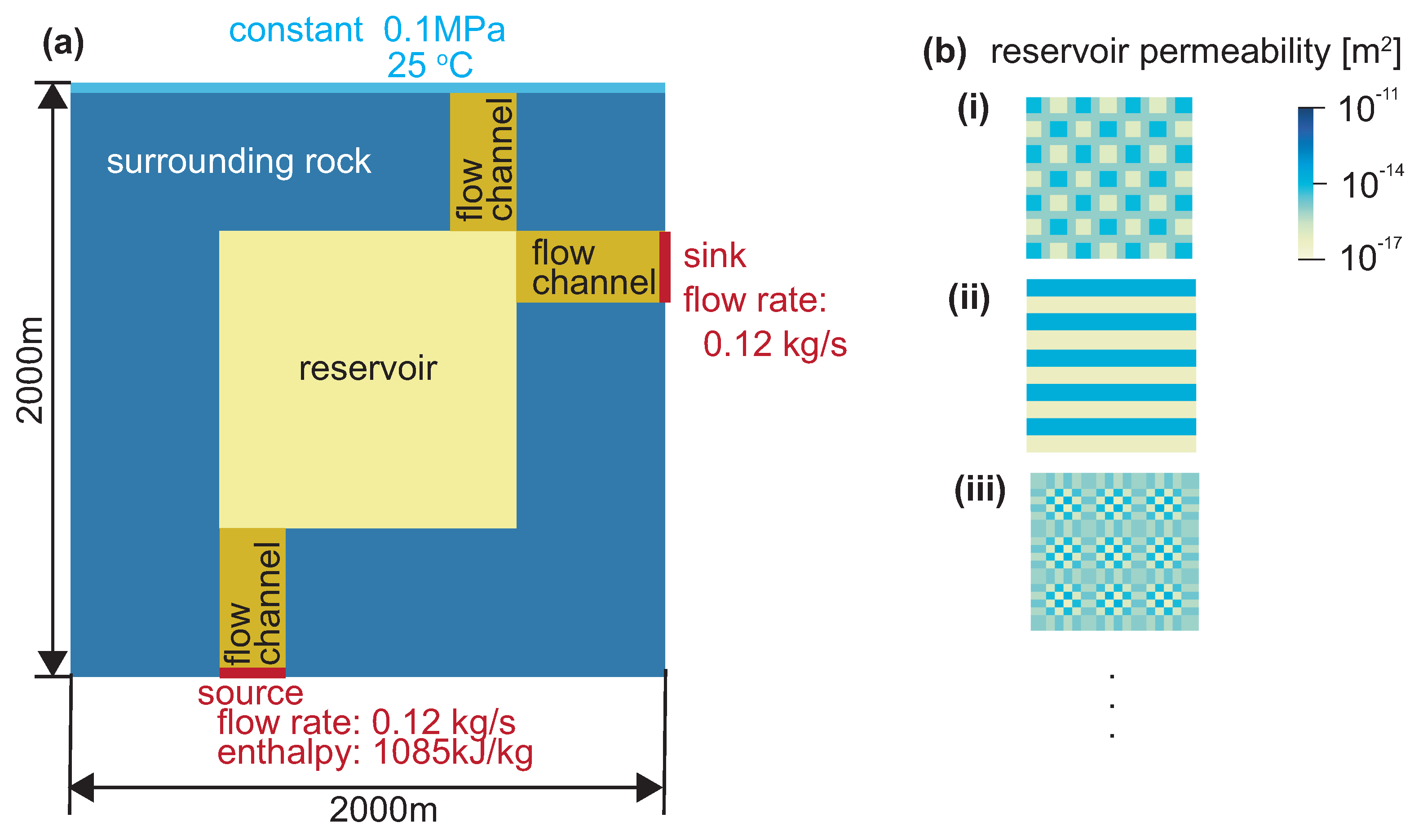
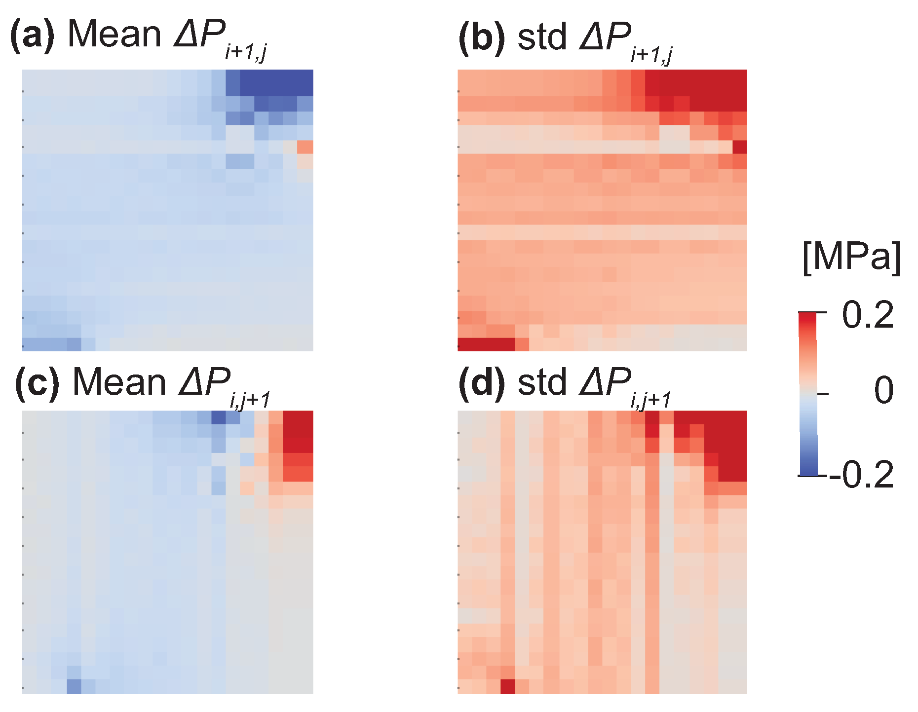
2.1. Preparation of Learning Data

In this study, we applied several popular machine-learning algorithms to estimate permeability distributions using measurable data in geothermal reservoir modeling. Here, we assume that two-dimensional temperature and pressure distributions of the area could be obtained from the temperature and pressure measured in multiple wells by using kriging or other methods.
First, we prepared large learning datasets from a numerical reservoir simulator TOUGH2, which simulates fluid and heat flow using the finite volume method [1]. Two-dimensional synthetic models were prepared with the simulation domain shown in Figure 1. The simulation area was 2000 m × 2000 m by 30 grids × 30 grids. The grids were discretized at 100 m in the center (20 grids × 20 grids) and at 50 m in the surrounding area. The top boundary was open boundary with temperature of 25 C and pressure of 0.1 MPa. The bottom and side boundaries were no flow condition except grids with sources and sinks. The heat source was located at the bottom left, and the sink was located at the right side, as shown in Figure 1. The simulation domain consisted of three areas: the surrounding rocks, the reservoir, and the flow channels. The heat source was connected to the reservoir area by the flow channels. The mass flow rate at the heat source was set to 0.12 kg/s, and the flowing specific enthalpy was 1085 kJ/kg (250 C for saturated water). The mass flow rate at the sink was set at 0.12 kg/s. The other input parameters for the simulation are listed in Table 1. It should be noted that porosity was set to constant because the effect of porosity is small on natural state simulation.
To prepare a large number of training data, different permeability patterns in the reservoir area were generated. The patterns were generated based on the discrete cosine transform, which is a basic image generation method used in image analysis [39]. The two-dimensionaldiscrete cosine transform is given by
X k 1 , k 2 = n 1 = 0 N 1 1 n 2 = 0 N 2 1 x n 1 , n 2 cos π N 2 n 2 + 1 2 k 2 cos π N 1 n 1 + 1 2 k 1 = n 1 = 0 N 1 1 n 2 = 0 N 2 1 x n 1 , n 2 cos π N 1 n 1 + 1 2 k 1 cos π N 2 n 2 + 1 2 k 2 for k 1 = 0 , , N 1 1 and k 2 = 0 , , N 2 1 .
where X is the image matrix of size N 2 by N 1 , and X k 1 , k 2 is the matrix element in X. The real numbers x 0 , 0 , , x N 1 1 , N 2 1 are transformed into the real numbers X 0 , 0 , , X N 1 1 , N 2 1 .Examples of generated permeability distributions based on the discrete cosine transform are shown in Figure 1b. Strip and lattice shapes can be seen. Note that the standard value of the permeability in the reservoir area was set to 10 15 m 2 , the permeability in the surrounding rocks was set to 10 18 m 2 , and the permeability in the flow channels was set to 10 15 m 2 . Here, some of the permeability distributions from the discrete cosine transform appear to be far from actual geological formations, but the structures close to the actual geology, such as layer formations, are also included in the training data. In particular, the machine learning method used in this project, as we explain later, does not grasp the overall trend of the distribution, but estimates the values based on local information. Therefore, even if some of the permeability distributions from discrete cosine transform seem geometric and unrealistic, we think the discrete cosine transform is fine for this project.
Two hundred permeability patterns were generated for each simulation. Each simulation was run for 10 14 s to reach the quasi-steady state, which is regarded as the natural state of geothermal reservoirs. Some of the simulations stopped before reaching the quasi-steady state. We used 180 simulation results of the simulations which continued until the end as the learning data.

2.2. Development of Machine Learning Model

The combination of permeability, temperature, and pressure distributions for 180 simulations was used for developing learning models. The variable being predicted is referred to as the “output” or “target”, while the input variables are referred to as “features”. In this study, the values of permeability in the reservoir domain were set as the target variables. The feature variables were given based on the values of the simulation outputs (i.e., temperature and pressure).
A regression analysis is a statistical method for modeling the relationship between targets and feature variables. Among the various types of regression algorithms for supervised machine learning, we applied the following in this study: a linear regression, a ridge regression, a Lasso regression, a support vector regression (SVR), a multilayer perceptron (MLP), a random forest, a gradient boosting, and a k-nearest neighbor algorithm. We used Python packages sklearn (v1.0.2), numpy (v1.22.1), optuna (v2.10.0), lightgbm (v3.3.2), and matplotlib (v3.0.3) in Python (v3.7.12).
The ridge regression and the Lasso regression, which are among the most robust versions of linear regression, introduce regularization techniques to reduce the complexity of the model [40,41]. The support vector machine (SVM) is a popular supervised machine learning algorithm and is representative of nonparametric machine learning methods [42]. We implemented the support vector regression (SVR) with the kernel functions of the linear, polynomial, and radial basis function (rbf). The multilayer perceptron (MLP) refers to a neural network of multiple formal neurons connected in multiple layers [43]. In the case of the random forest, a large number of decision trees are created by random sampling that allows for duplication, and the final prediction is determined by taking a majority vote of the prediction results obtained for each tree [44]. Gradient boosting continuously modifies and adds predictors to the ensemble, and also modifies the predictor to fit the residual error [45]. The k-nearest neighbor algorithm is a method based on the nearest training examples in the feature space [46]. We imported their modules from scikit-learn [47].
Two different approaches to building the models were applied. The first was to build a model with dependence on the grid. Each learning model was developed on each grid, and there were 400 learning models for each grid in the reservoir domain (20 grids × 20 grids). This type of model is referred as grid-dependent. The second was to build a model with no dependence on the grid. A single learning model was developed using data from all grids. This type of model is referred as grid-independent.
For both the grid-dependent model and grid-independent model, we first arranged the simulation results in a random order to separate the simulation results into a learning dataset and test dataset. The dataset of the first 70% of simulations was used as the training data, and the remaining 30% was used as the test data. The results of 180 simulations were divided into 126 simulations for use as the training data and 54 simulations for use as the test data.
The training dataset was normalized to adjust a wide numeric range of input variables to the range of [0, 1] using the minimum and maximum values of each feature variable. The normalized data was used to construct the learning model. Except for the linear regression, it was necessary to tune the hyperparameters. We used an automatic hyperparameter optimization software framework, Optuna [48], which is designed to automatically and efficiently search for optimal hyperparameters in large spaces. We performed a three-fold cross validation search for the hyperparameters. The hyperparameters and the range tuned in this study are listed in Table 2. The performance of the prediction model was scored by the coefficient of determination ( R 2 ).
After developing a learning model based on the training set, the learning model was evaluated with the test dataset. The test dataset was normalized with the scaling equation according to the attribute range of the training dataset with the best hyperparameters tuned with the training dataset.

3. Results

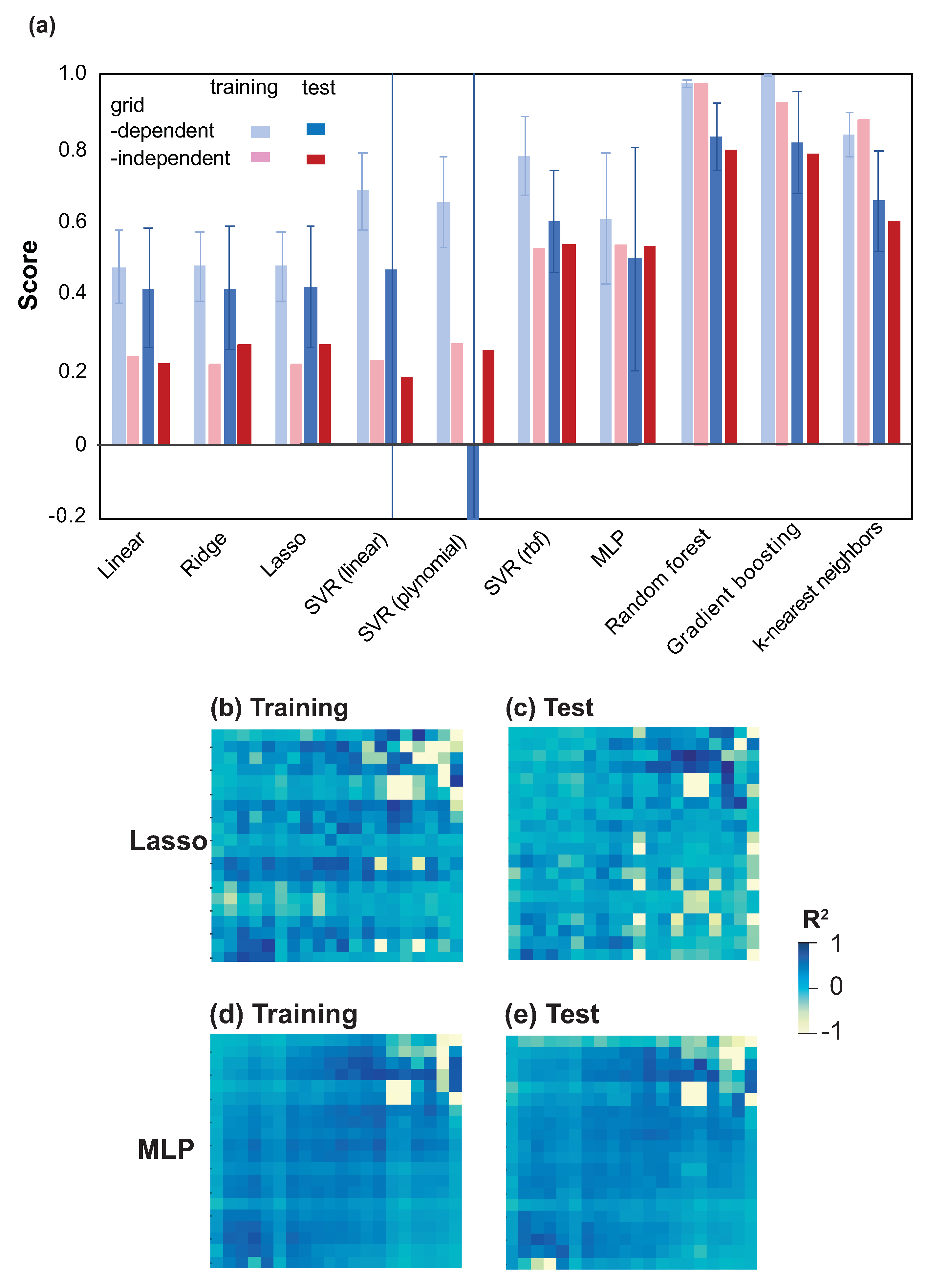
3.1. Model Selection

Selecting the feature variables is one of the core concepts in machine learning and has a large impact on the performance of the learning model [49]. We prepared 18 feature variables based on the temperature and pressure data given in Figure 2 to estimate the permeability of a grid point ( K i , j ) (Figure 2a). These features were the temperature of the point to be estimated ( T i , j ) (Figure 2b), the pressure of the point to be estimated ( P i , j ) (Figure 2c), and the temperature and pressure of the points adjacent to the point to be estimated in the x- and y-directions ( T i 1 , j , T i + 1 , j , T i , j 1 , T i , j + 1 , P i 1 , j , P i + 1 , j , P i , j 1 , P i , j + 1 ). In addition, we used the spatial differences in the temperature and pressure between the point to be estimated and the points adjacent to the point to be estimated in the x- and y-directions, which are denoted as Δ T i 1 , j , Δ T i + 1 , j , Δ T i , j 1 , Δ T i , j + 1 , Δ P i 1 , j , Δ P i + 1 , j , Δ P i , j 1 , Δ P i , j + 1 , as shown in Figure 2b,c. The grid numbers were assigned starting from the lower left of the computational domain, as shown in Figure 1a. Since the heat source was set to the lower left, the smaller grid number is considered to be upstream, and the larger grid number is considered to be downstream.
The importance of features is a measure of the extent to which feature partitioning contributes to the regression of the target. We calculated the impurity-based feature importances from scikit-learn modules with random forest [44]. The importances of feature variables for the grid-dependent models and for the grid-independent model are plotted in Figure 2d,e, respectively. For grid-dependent models, we plot their mean values and the standard deviation with error bars (Figure 2d). As shown in Figure 2d, the feature importance of the pressure difference with downwind in the x- and y-directions ( Δ P i + 1 , j , Δ P i , j + 1 ) was higher in both the grid-dependent models and the grid-independent model (Figure 2e).
It is important to note that rather than reflect the intrinsic predictive value of a particular feature by itself, the impurity-based feature importance indicates the importance of this feature for a particular model. In other words, the results obtained with random forest may not be applicable to other machine learning models. Nevertheless, it was clear that the pressure differences were more important than the other feature variables, as can be seen in Figure 2. In addition, when we consider the physical meaning of the feature variables, since permeability was used in the TOUGH2 with the Darcy law along with the pressure gradients [1], it is understandable that the pressure differences affect the flow conditions and can be more important than the other feature variables in estimating permeability.
The statistic values of pressure differences for each grid are shown in Figure 3. Figure 3a,b show the mean and standard deviation of pressure differences between adjacent grids in the x-direction, while Figure 3c,d show the mean and standard deviation of pressure differences between adjacent grids in the y-direction. As we can see, the values in the lower left and upper right of the region are larger or smaller than the others. The flow channels connecting to the heat source and sink were located near the bottom left and top right of the region. Because the flow channels were near the heat source and sink, the flow movement was rapid in these areas and the pressure difference was larger. Note also that trends in the results of the pressure differences upwind are similar to those downwind.
For both the grid-dependent and grid-independent models, the pressure differences downwind were more important than those upwind. Here, we observed that the accuracy of the model estimation was improved by using both the upwind and downwind pressure difference rather than only using the downwind pressure difference. When we prepare the pressure data, it is always possible to obtain the values of the downwind and upwind pressure differences. Thus, in the following results, we used the four pressure differences ( Δ P i 1 , j , Δ P i + 1 , j , Δ P i , j 1 , Δ P i , j + 1 ) as feature variables to build the learning model.
The different machine learning algorithms for the grid-dependent models and the grid-independent model were compared. We calculated the estimation scores as the coefficient of determination ( R 2 ). The results of the scores are plotted in Figure 4a. Since there were 400 results for the grid-dependent models, the means and the standard deviation with the error bars were plotted for the grid-dependent models, as shown in Figure 4a.
The linear, ridge, and Lasso models are based on a linear model. The obtained scores were lower than others (Figure 4a). The accuracy of the grid-dependent models based on their training data is better than that of the grid-independent model. The more diverse relationships between the feature and the target at different locations with different flow patterns in the independent model are more difficult to characterize in the linear models. This may explain the lower accuracy of the grid-independent model than that of the dependent model. The scores of training and test dataset using grid-independent model with Lasso, as an example of linear model, are shown in Figure 4b,c. The accuracy of the training data near the upper right was poor. In the upper right corner, water flowed out to the top and right boundaries due to the boundary setting in this study. This resulted in larger or smaller pressure differences, as shown in Figure 3a,c. It is expected that the flow movement was steeper than in other areas and that the linear model could not capture such different flow behaviors. In addition, the accuracy of the test data was poorer in the lower right areas. Since the pattern of the permeability distribution given by the discrete cosine transform appears to be reflected in the obtained scores, it is likely that the permeability distribution also affects the estimation accuracy. These results confirm that the simple linear model was not capable of dealing with the differences in flow patterns and differences in permeability distribution given by the discrete cosine transform.
Because SVR and MLP are nonlinear models, they are expected to be able to represent more complex relationships than the linear models. As expected, the training data for the grid-dependent model provided better scores. However, the test data for the grid-dependent SVR model with polynomial function showed very poor scores. When we observed the results of the scores in the spatial distribution, grids with poor prediction accuracy appeared randomly, which suggests that the heterogeneous permeability distributions given by the discrete cosine transform in the training data affected the accuracy of the learning model. There is a possibility that the accuracy can be improved by increasing the number of training data, but for the sake of comparison with other models, we used the same amount of training data to obtain the results in this study.
Although the scores of the nonlinear grid-independent models (SVR and MLP) were better than those of the linear models, the values of the test data stopped at about 0.5. The scores of the training and test dataset using the grid-independent model with MLP, as an example of a nonlinear model, are shown in Figure 4d,e. The accuracy of the training data near the upper right was poor, and was similar to the score obtained by the Lasso model. Nonlinear models do not characterize the features well with discontinuities in the mapping function. The large difference in the pressure differences between the center area and the upper right area suggests that the mapping function with the feature variables may be discontinuous. This may explain the poor results obtained by the test data in the grid-dependent model for the nonlinear models.
The scores of random forest and gradient boosting were almost 1.0 for the training dataset and around 0.8 for the test dataset. Random forest and gradient boosting are based on ensembles (approximation with multiple functions), and may be suitable even in cases where the mapping function is discontinuous.
In random forest and gradient boosting, although the performance of the grid-dependent models was better than the grid-independent model, the difference was small. Because it is easier to prepare the training data in the grid-independent model, it may be able to be used in different model settings, such as different positions of the source and sink in the boundary conditions. We adopted the grid-independent model with a random forest algorithm in this study.

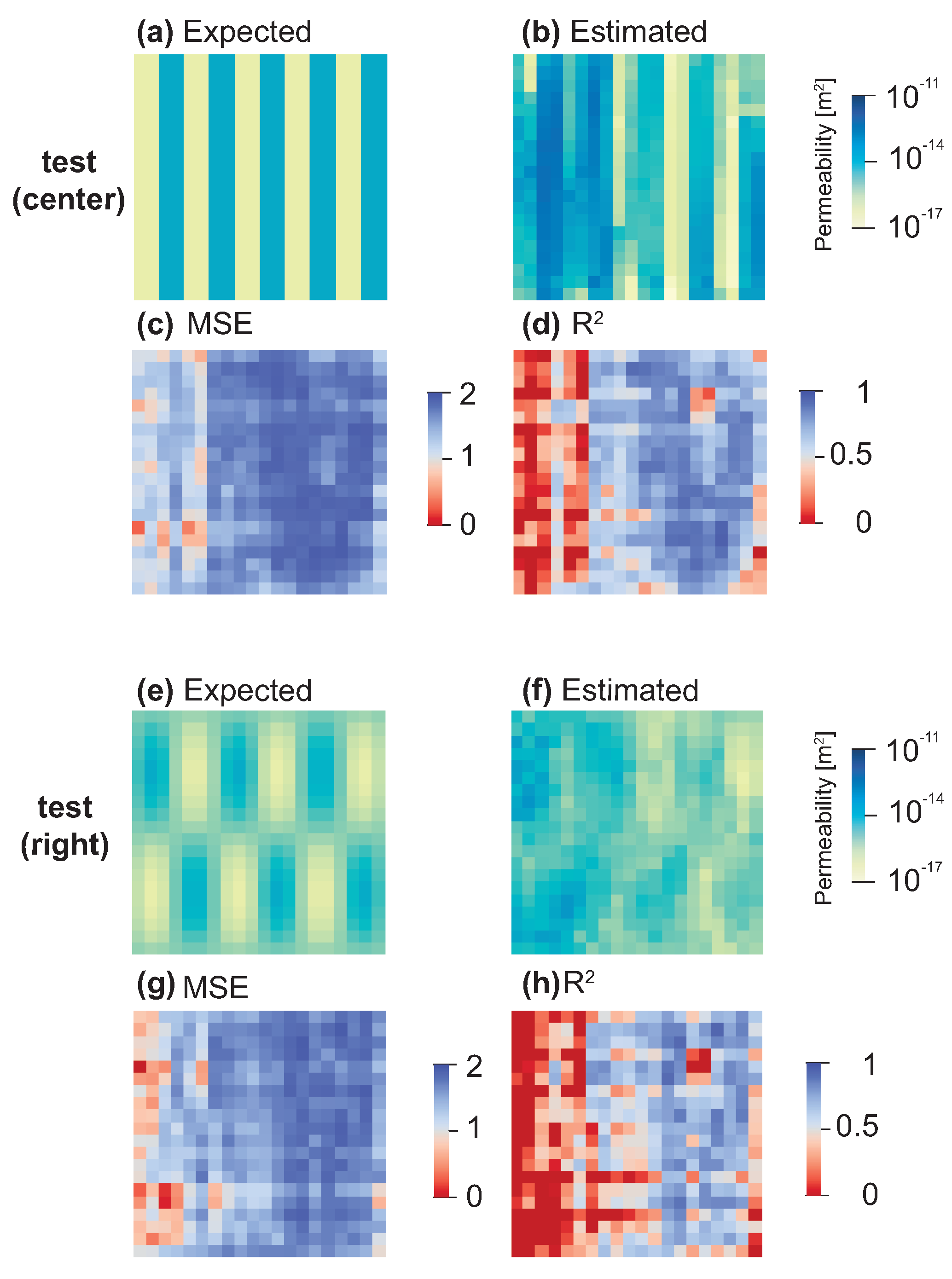
3.2. Estimation of Permeability Distributions

The results of the permeability estimation for the training dataset using the the grid-independent model with the random forest algorithm are shown in Figure 5. Among the results obtained for 126 simulations using the training dataset, we show two examples of permeability patterns (Figure 5a,c) and their estimation results (Figure 5b,d), which were selected randomly from among all the simulation results. Figure 5e plots the spatial distribution of the mean of the squared error (MSE) between the expected values and the estimated values for each grid for the training dataset. In Figure 5f, the spatial distribution of the coefficient of determination ( R 2 ) is shown for the expected and estimated values for each grid. There was almost no error, and the expected and estimated values are highly correlated. The score was calculated by using the coefficient of determination ( R 2 ). The score for the training dataset was 0.979, as listed in Table 3.
The results of the estimation for the test dataset are shown in Figure 6 for two examples of permeability patterns (Figure 6a,c) and their estimation results (Figure 6b,d). Although some parts were not perfectly estimated, the estimation captured most of the trends in the permeability distribution. This indicates that this learning model can be applied to the test dataset.
Figure 6e,f are plots of the spatial distributions of the mean of the squared error and R 2 between the expected values and the estimated values for each grid for test dataset. As shown in Figure 6e,f, near the center of the domain, the error was small and the expected and estimated values were highly correlated. On the other hand, the estimation accuracy at the top and left edges appeared to be degraded. Since the heat source was placed in the bottom left corner, the estimation of the area distant from the heat source may have been compromised. The score was 0.789.

3.3. Estimation for Different Heat Source Conditions

In the previous subsection, it was shown that the grid-independent model with random forest algorithm can estimate permeability distributions for the test dataset. The above test data were obtained from a reservoir model in which only the permeability distribution was changed from the training data. When preparing a reservoir model, in addition to the permeability distribution, settings of the conditions of the heat source and sink may also have large impacts on the simulation results. Therefore, in this subsection, we examine whether the training model can be applied to a test dataset generated under different source and sink conditions.
First, the effects of the magnitude of the mass flow rate at the source were investigated. The simulations were performed with different patterns of permeability and varied mass flow rates of 0.04, 0.12, and 0.4 kg/s, respectively. The simulation results at the mass flow rate of 0.12 kg/s were used as the training data. These results are the same as those shown in Figure 6. In order to compare the results with the test data at the mass flow rate of 0.12 kg/s, 30% of the total data was also used as the test data for the mass flow rates of 0.04 and 0.4 kg/s.
Figure 7 shows the estimation results for test dataset prepared using different source mass flow rates. Figure 7a,b show plots of an example of permeability distribution and their estimation results for mass flow rate of 0.04 kg/s, and Figure 7c,d are plots of the spatial distributions of the mean of the squared error and R 2 between the expected values and the estimated values for each grid. Figure 7e–h show the results for the test case for mass flow rate of 0.4 kg/s. In the case of the mass flow rate of 0.04 kg/s, the errors at the bottom left corner were relatively high, and the errors at the mass flow rate of 0.4 kg/s were relatively high at the bottom right corner. Nevertheless, we can see that the middle of the reservoir region was estimated with good accuracy. The scores for the test dataset with mass flow rate of 0.04 kg/s and 0.4 kg/s were 0.715 and 0.768, respectively, as listed in Table 3. There was little difference between those scores and the score for the test dataset with the same conditions as the training dataset ( R 2 = 0.789). This suggests that the learning model can be applied to reservoir models with different mass flow rates to the training data.
Next, the effect of positions of the heat source was investigated. The simulations were performed with different patterns of permeability with different positions of heat sources. The learning dataset was generated by setting the heat source on the bottom left of the reservoir, as shown in Figure 1a. Here, we prepared the test dataset with the heat source positioned at the bottom center and the bottom right, as shown in Figure 8a,b. The simulation results with the source locating at the bottom left were used as the training data, while the simulation results with source locating at the bottom left, bottom center, and bottom right were used as the test data.
Figure 9 show the estimation results for the test dataset prepared using different locations of heat source. Figure 9a,b show plots of an example of permeability distribution and their estimation results when the heat source was located on the center bottom, and Figure 9c,d are plots of the spatial distributions of the mean of the squared error and R 2 between the expected values and the estimated values for each grid. Figure 9e–h show the results for the test case when the heat source was located on the right bottom. It can be observed that as the heat source shifted to the right, the estimation accuracy of the left side of the reservoir region decreased. The scores for the test dataset where the source position was center and right were 0.576 and 0.450, respectively, as listed in Table 3. The more the source position deviated from the training data, the worse the test data score became. Since the sink was placed at the upper right of the reservoir, the main water flow was from the bottom left (the heat source) to the top right (the sink). When the heat source was located at the bottom right, the left side of the reservoir region is considered to have had less water movement. In this case, even if the permeability was high, the lack of water movement would lead to underestimations of permeability. The low accuracy of the estimation at the left side of the reservoir area may be attributed to this lack of water movement.
We have shown that the learning model developed in this study can be used to estimate most of the trends of permeability, indicating that the estimation works well even when for different positions of sources. In order to further improve the accuracy, we intend to develop a learning model that can estimate the source and sink conditions in future research. For application to objects with different conditions, the application of data augmentation and domain adaptation need to be considered as future tasks. Both of these have been shown to be effective in deep learning [50,51].

4. Discussion

The machine learning approach proposed in this study directly estimates input parameters in the reservoir model from measurable data. This eliminates the need for a trial-and-error search for input parameters in the reservoir modeling, which is a major challenge in conventional modeling approaches. Of course, inverse analysis methods developed in the past (e.g., iTOUGH2 [14]) could also provide good estimates. Although we have not compared the accuracy of the estimation between inverse analysis methods and our approach, the estimation accuracy may be better in both cases, depending on the optimization. On the other hand, the good point of our approach is that once the learning model is created, it does not need to be computed over and over again, and it can be used even on computers with low specifications. This would help to expand the spread of small fields, which cannot be developed with large amounts of equipment. It also provides reliable reservoir modeling which does not rely on the experience and intuition of analysts. This allows non-experienced developers to work on reservoir modeling and helps to create an environment where new people can take part in geothermal development. Reservoir modeling is one of the most important challenges in making strategies for geothermal reservoir development. Improvements in the reliability of reservoir modeling are expected to greatly accelerate the geothermal development.
Geothermal developments cannot drill a large number of wells due to the drilling cost. Thus, the pressure data in the natural state is only available for the discrete data from the limited wells. The learning model proposed in this study, however, requires two-dimensional pressure distributions. If we apply our method to field data, it is necessary to measure the pressure from at least three points surrounding the target surface for the 2D estimation and to interpolate the discrete data by interpolation techniques, such as kriging (e.g., [52]). Future research will examine the estimation errors when interpolations are performed.
In addition, when not many data points are available, as in the case of geothermal development, it is important to evaluate carefully how uncertain the measurements based on the data are. To evaluate the impacts of the uncertainties on the estimation, uncertainty quantification methods, such as Bayesian approximation and ensemble learning techniques (e.g., [53]), play some pivotal roles. Combining uncertainty quantification with our approach is also desirable for future study.
This study is limited to numerical experiments and has not been applied to actual field data. At present, a model for two-dimensional data has been developed, but a model for three-dimensional data is expected to be developed, assuming the actual field. In addition, our simulation was limited to thermohydraulic simulation as a first step to develop the machine learning approach. To make our analysis available for real field development, 3D thermohydraulic–mechanical–chemical simulations are needed in the next research.
This study applied several regression models in machine learning to estimate the permeability based on the two-dimensional distributed features. Two-dimensional image recognition can be powerfully trained by convolutional neural networks (CNNs) [54], and the application of CNNs should be considered in future research.
Our approach is similar to data-driven physics-informed machine learning to search for new governing equations of physical phenomena, which has been a hot topic in the field of machine learning (e.g., [55,56,57]). Although such approaches are still only applied to basic science, they are expected to be developed in the fields of Earth science and energy resource engineering. In this study, we successfully demonstrated the first step toward the goal of achieving a new data-driven geothermal reservoir engineering, which will be developed and enhanced by incorporating information science.

5. Conclusions

We developed a machine learning model to uniquely estimate input parameters based on measured data in order to improve the conventional reservoir modeling approach, which determines the input parameters by trial and error. In this study, the relationship between the measurement data and permeability, one of the most important input parameters in reservoir modeling, was successfully determined by machine learning. First, we generated a large number of permeability distributions based on the discrete cosine transform and conducted natural state simulations using each permeability distribution. The simulation results of pressure and temperature distributions were used for feature variables. We used several popular supervised machine learning approaches: the linear regression, the ridge regression, the Lasso regression, the support vector regression (SVR), multilayer perceptron (MLP), random forest, gradient boosting, and the k-nearest neighbor algorithm. Learning models were developed both with and without the dependence of the grids. The results showed that the grid-independent model by random forest with the pressure differences as feature variables provided good estimations of permeability. It was also found that the model could be applied to the test dataset with different mass flow rates of the heat sources. The estimation became more difficult when the position of the source was different. However, the estimation was successful for the region with a flow field even when the position of the source was different. We successfully demonstrated the first step toward the goal of achieving new data-driven geothermal reservoir engineering, which will be developed and enhanced by incorporating information science.

Author Contributions

Conceptualization, A.S. and T.H.; methodology, K.-i.F. and A.S.; software, validation, formal analysis, investigation, data curation, writing—original draft preparation, visualization, A.S.; writing—review and editing, K.-i.F., S.O., J.I. and T.H.; project administration, T.H.; funding acquisition, A.S. and T.H. All authors have read and agreed to the published version of the manuscript.

Funding

This research was funded by JSPS KAKENHI Grant Numbers JP20H02676 (Japan) and JST ACT-X Grant Number JPMJAX190H (Japan).

Institutional Review Board Statement

Not applicable.

Informed Consent Statement

Not applicable.

Data Availability Statement

The datasets generated in this study and the program code are available from the authors on a reasonable request.

Acknowledgments

We We would like to thank the members in Joint Research program 2021-B-01 and 2018-B-01 for useful discussions.

Conflicts of Interest

The authors declare that they have no known competing financial interests or personal relationships that could have appeared to influence the work reported in this paper. This study was supported by Tohoku Electric Power Co., Inc., of whom Shinya Onodera and Junichi Ishizaki are employees. The company and the funders had no role in the design of the study; in the collection, analyses, or interpretation of data; in the writing of the manuscript, or in the decision to publish the results.

References

  1. Pruess, K.; Oldenburg, C.M.; Moridis, G.J. TOUGH2 User’s Guide, version 2; LBNL-43134; Lawrence Berkeley National Lab.: Berkeley, CA, USA, 1999. [Google Scholar]
  2. Vinsome, K.; Shook, M. Multi-purpose simulation. J. Pet. Sci. Eng. 1993, 9, 29–38. [Google Scholar] [CrossRef]
  3. Pritchett, J.W. STAR: A geothermal reservoir simulation system. In Proceedings of the World geothermal Congress, Florence, Italy, 18–31 May 1995; pp. 2959–2963. [Google Scholar]
  4. Keller, J.; Rath, V.; Bruckmann, J.; Mottaghy, D.; Clauser, C.; Wolf, A.; Seidler, R.; Bücker, H.M.; Klitzsch, N. SHEMAT-Suite: An open-source code for simulating flow, heat and species transport in porous media. SoftwareX 2020, 12, 100533. [Google Scholar] [CrossRef]
  5. Hughes, J.; Langevin, C.; Banta, E. Documentation for the MODFLOW 6 framework. In USGS: Techniques and Methods 6-A57; U.S. Geological Survey: Reston, VA, USA, 2017; p. 42. [Google Scholar]
  6. Mahmoodpour, S.; Singh, M.; Turan, A.; Bär, K.; Sass, I. Hydro-Thermal Modeling for Geothermal Energy Extraction from Soultz-sous-Forêts, France. Geosciences 2021, 11, 464. [Google Scholar] [CrossRef]
  7. Ganguly, S.; Kumar, M.S. Geothermal reservoirs—A brief review. J. Geol. Soc. India 2012, 79, 589–602. [Google Scholar] [CrossRef] [Green Version]
  8. Pratama, H.B.; Saptadji, N.M. Numerical simulation for natural state of two-phase liquid dominated geothermal reservoir with steam cap underlying brine reservoir. IOP Conf. Ser. Earth Environ. Sci. 2016, 42, 012006. [Google Scholar] [CrossRef]
  9. Manggala Putra, R.P.; Sutopo, S.; Pratama, H.B. Improved natural state simulation of Arjuno-Welirang Geothermal field, East Java, Indonesia. IOP Conf. Ser. Earth Environ. Sci. 2019, 254, 012022. [Google Scholar] [CrossRef]
  10. Jalilinasrabady, S.; Tanaka, T.; Itoi, R.; Goto, H. Numerical simulation and production prediction assessment of Takigami geothermal reservoir. Energy 2021, 236, 121503. [Google Scholar] [CrossRef]
  11. Grant, M.A.; Bixley, P.F. Geothermal Reservoir Engineering, 2nd ed.; Academic Press: Oxford, UK, 2011; p. 378. [Google Scholar]
  12. Finsterle, S.; Pruess, K. Development of Inverse Modeling Techniques for Geothermal Applications; LBNL-40039; Lawrence Berkeley Lab.: Berkeley, USA, 1997; p. 8. [Google Scholar]
  13. O’Sullivan, M.J.; Pruess, K.; Lippmann, M.J. State of the art of geothermal reservoir simulation. Geothermics 2001, 30, 395–429. [Google Scholar] [CrossRef]
  14. Finsterle, S. iTOUGH2 User’s Guide; LBNL-40040; Lawrence Berkeley Lab.: Berkeley, CA, USA, 2007; p. 137. [Google Scholar]
  15. Poeter, E.P.; Hill, M.C. UCODE, a computer code for universal inverse modeling. Comput. Geosci. 1999, 25, 457–462. [Google Scholar] [CrossRef]
  16. Doherty, J. Calibration and uncertainty analysis for complex environmental models. Groundwater 2015, 53, 673–674. [Google Scholar] [CrossRef]
  17. Bjarkason, E.K.; O’Sullivan, J.P.; Yeh, A.; O’Sullivan, M.J. Inverse modeling of the natural state of geothermal reservoirs using adjoint and direct methods. Geothermics 2019, 78, 85–100. [Google Scholar] [CrossRef]
  18. Assouline, D.; Mohajeri, N.; Gudmundsson, A.; Scartezzini, J.L. A machine learning approach for mapping the very shallow theoretical geothermal potential. Geotherm. Energy 2019, 7, 19. [Google Scholar] [CrossRef] [Green Version]
  19. Spichak, V.; Geiermann, J.; Zakharova, O.; Calcagno, P.; Genter, A.; Schill, E. Estimating deep temperatures in the Soultz-sous-Forêts geothermal area (France) from magnetotelluric data. Near Surf. Geophys. 2015, 13, 397–408. [Google Scholar] [CrossRef]
  20. Ishitsuka, K.; Kobayashi, Y.; Watanabe, N.; Yamaya, Y.; Bjarkason, E.; Suzuki, A.; Mogi, T.; Asanuma, H.; Kajiwara, T.; Sugimoto, T.; et al. Bayesian and neural network approaches to estimate deep temperature distribution for assessing a supercritical geothermal system: Evaluation using a numerical model. Nat. Resour. Res. 2021, 30, 3289–3314. [Google Scholar] [CrossRef]
  21. Rezvanbehbahani, S.; Stearns, L.A.; Kadivar, A.; Walker, J.D.; van der Veen, C.J. Predicting the geothermal heat flux in Greenland: A machine learning approach. Geophys. Res. Lett. 2017, 44, 12271–12279. [Google Scholar] [CrossRef] [Green Version]
  22. Siler, D.L.; Pepin, J.D.; Vesselinov, V.V.; Mudunuru, M.K.; Ahmmed, B. Machine learning to identify geologic factors associated with production in geothermal fields: A case-study using 3D geologic data, Brady geothermal field, Nevada. Geotherm. Energy 2021, 9, 17. [Google Scholar] [CrossRef]
  23. Gudmundsdottir, H.; Horne, R.N. Prediction modeling for geothermal reservoirs using deep learning. In Proceedings of the 45th Workshop on Geothermal Reservoir Engineering, Stanford University, Stanford, CA, USA, 10–12 February 2020; p. 12. [Google Scholar]
  24. Holtzman, B.K.; Paté, A.; Paisley, J.; Waldhauser, F.; Repetto, D. Machine learning reveals cyclic changes in seismic source spectra in Geysers geothermal field. Sci. Adv. 2018, 4, eaao2929. [Google Scholar] [CrossRef] [PubMed] [Green Version]
  25. Gao, K.; Huang, L.; Lin, R.; Hu, H.; Zheng, Y.; Cladohous, T. Delineating faults at the soda lake geothermal field using machine learning. In Proceedings of the 46th Workshop on Geothermal Reservoir Engineering, Stanford University, Stanford, CA, USA, 16–18 February 2021; p. 8. [Google Scholar]
  26. Zheng, Y.; Li, J.; Lin, R.; Hu, H.; Gao, K.; Huang, L.; Sciences, A.; Alamos, L. Physics-Guided Machine Learning Approach to Characterizing Small-Scale Fractures in Geothermal Fields. In Proceedings of the 46th Workshop on Geothermal Reservoir Engineering, Stanford University, Stanford, CA, USA, 16–18 February 2021; p. 9. [Google Scholar]
  27. Ali, S.S.; Nizamuddin, S.; Abdulraheem, A.; Hassan, M.R.; Hossain, M.E. Hydraulic unit prediction using support vector machine. J. Pet. Sci. Eng. 2013, 110, 243–252. [Google Scholar] [CrossRef]
  28. Al-Mudhafar, W.J. Integrating well log interpretations for lithofacies classification and permeability modeling through advanced machine learning algorithms. J. Pet. Explor. Prod. Technol. 2017, 7, 1023–1033. [Google Scholar] [CrossRef] [Green Version]
  29. Anifowose, F.; Abdulraheem, A.; Al-Shuhail, A. A parametric study of machine learning techniques in petroleum reservoir permeability prediction by integrating seismic attributes and wireline data. J. Pet. Sci. Eng. 2019, 176, 762–774. [Google Scholar] [CrossRef]
  30. Erofeev, A.; Orlov, D.; Ryzhov, A.; Koroteev, D. Prediction of porosity and permeability alteration based on machine learning algorithms. Transp. Porous Media 2019, 128, 677–700. [Google Scholar] [CrossRef] [Green Version]
  31. Kaydani, H.; Mohebbi, A.; Eftekhari, M. Permeability estimation in heterogeneous oil reservoirs by multi-gene genetic programming algorithm. J. Pet. Sci. Eng. 2014, 123, 201–206. [Google Scholar] [CrossRef]
  32. Sudakov, O.; Burnaev, E.; Koroteev, D. Driving digital rock towards machine learning: Predicting permeability with gradient boosting and deep neural networks. Comput. Geosci. 2019, 127, 91–98. [Google Scholar] [CrossRef] [Green Version]
  33. Al-Anazi, A.F.; Gates, I.D. Support vector regression for porosity prediction in a heterogeneous reservoir: A comparative study. Comput. Geosci. 2010, 36, 1494–1503. [Google Scholar] [CrossRef]
  34. Mo, S.; Zabaras, N.; Shi, X.; Wu, J. Deep autoregressive neural networks for high-dimensional inverse problems in groundwater contaminant source identification. Water Resour. Res. 2019, 55, 3856–3881. [Google Scholar] [CrossRef] [Green Version]
  35. Wen, G.; Tang, M.; Benson, S.M. Multiphase flow prediction with deep neural networks. arXiv 2019, arXiv:1910.09657. [Google Scholar] [CrossRef]
  36. Tang, M.; Liu, Y.; Durlofsky, L.J. A deep-learning-based surrogate model for data assimilation in dynamic subsurface flow problems. J. Comput. Phys. 2020, 413, 109456. [Google Scholar] [CrossRef] [Green Version]
  37. Jin, Z.L.; Liu, Y.; Durlofsky, L.J. Deep-learning-based surrogate model for reservoir simulation with time-varying well controls. J. Pet. Sci. Eng. 2020, 192, 107273. [Google Scholar] [CrossRef]
  38. Liu, Y.; Durlofsky, L.J. 3D CNN-PCA: A deep-learning-based parameterization for complex geomodels. Comput. Geosci. 2021, 148, 104676. [Google Scholar] [CrossRef]
  39. Ahmed, N.; Natarajan, T.; Rao, K.R. Discrete cosine transform. IEEE Trans. Comput. 1974, C-23, 90–93. [Google Scholar] [CrossRef]
  40. Hoerl, A.E.; Kennard, R.W. Ridge regression: Biased estimation for nonorthogonal problems. Technometrics 1970, 12, 55–67. [Google Scholar] [CrossRef]
  41. Tibshirani, R. Regression shrinkage and selection via the lasso. J. R. Stat. Soc. Ser. B (Methodol.) 1996, 58, 267–288. [Google Scholar] [CrossRef]
  42. Vapnik, V. The Nature of Statistical Learning Theory, 2nd ed.; Springer Science & Business Media: Berlin/Heidelberg, Germany; Springer: New York, NY, USA, 2000. [Google Scholar] [CrossRef]
  43. Orr, G.B.; Müller, K.R. Neural Networks: Tricks of the Trade, 2nd ed.; Springer: Berlin/Heidelberg, Germany, 2012. [Google Scholar] [CrossRef]
  44. Breiman, L. Random forests. Mach. Learn. 2001, 45, 5–32. [Google Scholar] [CrossRef] [Green Version]
  45. Mason, L.; Baxter, J.; Bartlett, P.; Frean, M. Boosting algorithms as gradient descent in function space. Proc. NIPS 1999, 12, 512–518. [Google Scholar] [CrossRef]
  46. Peterson, L.E. K-nearest neighbor. Scholarpedia 2009, 4, 1883. [Google Scholar] [CrossRef]
  47. Pedregosa, F.; Varoquaux, G.; Gramfort, A.; Michel, V.; Thirion, B.; Grisel, O.; Blondel, M.; Prettenhofer, P.; Weiss, R.; Dubourg, V.; et al. Scikit-learn: Machine learning in Python. J. Mach. Learn. Res. 2011, 12, 2825–2830. [Google Scholar] [CrossRef]
  48. Akiba, T.; Sano, S.; Yanase, T.; Ohta, T.; Koyama, M. Optuna: A next-generation hyperparameter optimization framework. In Proceedings of the 25th ACM SIGKDD International Conference on Knowledge Discovery & Data Mining (KDD ’19), Association for Computing Machinery, Anchorage, AK, USA, 4–8 August 2019; pp. 2623–2631. [Google Scholar] [CrossRef]
  49. Guyon, I.; Elisseeff, A. An introduction to variable and feature selection. J. Mach. Learn. Res. 2003, 3, 1157–1182. [Google Scholar] [CrossRef]
  50. Shorten, C.; Khoshgoftaar, T.M. A survey on image data augmentation for deep learning. J. Big Data 2019, 6, 60. [Google Scholar] [CrossRef]
  51. Zhao, S.; Yue, X.; Zhang, S.; Li, B.; Zhao, H.; Wu, B.; Krishna, R.; Gonzalez, J.E.; Sangiovanni-Vincentelli, A.L.; Seshia, S.A.; et al. A review of single-source deep unsupervised visual domain adaptation. IEEE Trans. Neural Netw. Learn. Syst. 2022, 33, 473–493. [Google Scholar] [CrossRef]
  52. Teng, Y.; Koike, K. Three-dimensional imaging of a geothermal system using temperature and geological models derived from a well-log dataset. Geothermics 2007, 36, 518–538. [Google Scholar] [CrossRef]
  53. Jiang, Z.; Zhang, S.; Turnadge, C.; Xu, T. Combining autoencoder neural network and Bayesian inversion to estimate heterogeneous permeability distributions in enhanced geothermal reservoir: Model development and verification. Geothermics 2021, 97, 102262. [Google Scholar] [CrossRef]
  54. Lawrence, S.; Giles, C.L.; Tsoi, A.C.; Back, A.D. Face recognition: A convolutional neural-network approach. IEEE Trans. Neural Netw. 1997, 8, 98–113. [Google Scholar] [CrossRef] [PubMed] [Green Version]
  55. Champion, K.; Lusch, B.; Nathan Kutz, J.; Brunton, S.L. Data-driven discovery of coordinates and governing equations. Proc. Natl. Acad. Sci. USA 2019, 116, 22445–22451. [Google Scholar] [CrossRef] [PubMed] [Green Version]
  56. Raissi, M.; Yazdani, A.; Karniadakis, G.E. Hidden fluid mechanics: Learning velocity and pressure fields from flow visualizations. Science 2020, 367, 1026–1030. [Google Scholar] [CrossRef] [PubMed]
  57. Harp, D.R.; O’Malley, D.; Yan, B.; Pawar, R. On the feasibility of using physics-informed machine learning for underground reservoir pressure management. Expert Syst. Appl. 2021, 178, 115006. [Google Scholar] [CrossRef]
Figure 1. Simulation condition. (a) Simulation area with boundary conditions. (b) Examples of permeability distribution patterns in the reservoir area. The patterns were generated using a discrete cosine transformation. (b) (i–iii) depicts three different patterns.
Geosciences 12 00130 g001
Figure 2. (ac) Setting of feature variables: (a) permeability K i , j , (b) temperature T i , j , and (c) pressure P i , j for grid x = i and y = j . (d,e) Results of relative importance of feature variables based on training data with random forest for (d) grid-dependent models and (e) grid-independent model.
Geosciences 12 00130 g002
Figure 3. Spatial distributions of mean and standard deviation of pressure differences with downwind for each grid. (a,c) The mean and (b,d) standard deviation (std) of Δ P i + 1 , j and Δ P i , j + 1 .
Geosciences 12 00130 g003
Figure 4. (a) Comparison of scores (coefficient of determination: R 2 ) for different methods. (b) Training and (c) test scores of Lasso model and (d) Training and (e) test scores of MLP model.
Geosciences 12 00130 g004
Figure 5. Results of permeability estimation for training dataset. Examples of (a,c) expected distributions and (b,d) estimated results. Spatial error distributions with (e) MSE and (f) R 2 .
Geosciences 12 00130 g005
Figure 6. Results of permeability estimation for test dataset. Examples of (a,c) expected distributions and (b,d) estimated results and spatial error distributions by (e) MSE and (f) coefficient of determination R 2 .
Geosciences 12 00130 g006
Figure 7. Estimation accuracy in the case of different mass flow rates at the source from the training data. (a) Expected vs. (b) estimated values, and spatial distributions of (c) MSE and (d) R 2 for the mass flow rate of 0.04 kg/s. (e) Expected vs. (f) estimated values, and spatial distributions of (g) MSE and (h) R 2 for the mass flow rate of 0.4 kg/s.
Geosciences 12 00130 g007
Figure 8. Setting of locations of heat sources for test data.The positions of heat sources are set to (a) bottom center and (b) bottom right.
Geosciences 12 00130 g008
Figure 9. Estimation accuracy in the case of different source locations from the training data. (a) Expected vs. (b) estimated values, and spatial distributions of (c) MSE and (d) R 2 when the heat source was located at the bottom center. (e) Expected vs. (f) estimated values, and spatial distributions of (g) MSE and (h) R 2 when the heat source was located at the bottom right.
Geosciences 12 00130 g009
Table 1. Input parameters in TOUGH2.
MethodsParametersSI Unit
Rock density2250kg/m 3
Porosity0.1-
Thermal conductivity2.5W/m C
Specific heat1000J/kg C
Table 2. Hyperparameters in each model.
MethodsParametersRanges
Linear--
Ridge α 0.00001–100
Lasso α 0.00001–100
max iteration100,000
SVR (linear)C0.01–10,000
SVR (polynomial)C0.01–10,000
degree2–4
SVR (rbf)C0.01–10,000
γ 0.0001–100
ϵ 0.0001–0.01
MLPsolversgd, adam, lbfgs
activationidentity, logistic,
relu, tanh
max layer size50–300
α 0.001–1000
Random forestnumber of trees in the forest100–1000
Gradient boostingnumber of boosting stages to perform100–1000
maximum depth3
k-nearest neighborsnumber of neighbors3–7
Table 3. Scores for training and test datasets. * Represents the same conditions as the training datasets.
Conditions
Mass Flow Rate (kg/s)PositionScore (R2)
Training0.12left0.979
Test0.12 *left *0.789
0.04left *0.715
0.4left *0.768
0.12 *center0.576
0.12 *right0.450
Publisher’s Note: MDPI stays neutral with regard to jurisdictional claims in published maps and institutional affiliations.

