
Receiver Function Imaging of the Crustal Structure Beneath Northern Taiwan Using Dense Linear Arrays


1
Institute of Seismology, National Chung Cheng University, Chiayi 62102, Taiwan
2
Institute of Earth Sciences, Academia Sinica, Taipei 11529, Taiwan
*
Author to whom correspondence should be addressed.
Geosciences 2022, 12(3), 136; https://0-doi-org.brum.beds.ac.uk/10.3390/geosciences12030136
Submission received: 16 February 2022
/
Revised: 11 March 2022
/
Accepted: 14 March 2022
/
Published: 15 March 2022
(This article belongs to the Section Geophysics)
Abstract
:In order to realize the crustal structure in Taiwan, the receiver function method was used to analyze the teleseismic waveforms recorded by two orthogonal broadband linear arrays deployed in northern Taiwan in the east–west and south–north directions by the TAiwan Integrated GEodynamics Research (TAIGER) project from 2007 to 2009. By incorporation with Common Conversion Point (CCP) stacking, the Moho discontinuities beneath northern Taiwan were imaged. Based on the CCP stack of receiver functions in the east–west direction array, a collision boundary between the Philippine Sea Plate and the Eurasian Plate appears at the east of Taiwan. The Moho depth of the Eurasian Plate in west Taiwan is flat and 30 km; the Moho depth of the Philippine Sea Plate below the Central Mountain Range is about 55 km; in the east, the Moho depth of the Ryukyu arc is about 40 km. The south–north profile shows a brittle–ductile transition zone at depths of 15–20 km beneath central Taiwan from south to north. Moreover, the Moho depth of the Eurasian Plate is about 20–25 km in northern Taiwan. The Moho depth appears to deepen from north to south. The deepest Moho is located at the junction of the two profile lines, the Philippine Sea Plate, and has a depth of 60 km. According to these Moho depths, the crustal structure is thin and flat in the west part of northern Taiwan which is similar to the thin-skin model. However, the lithosphere is deformed and forms the mountain root in the east part which is similar to the lithospheric collision model.
1. Introduction
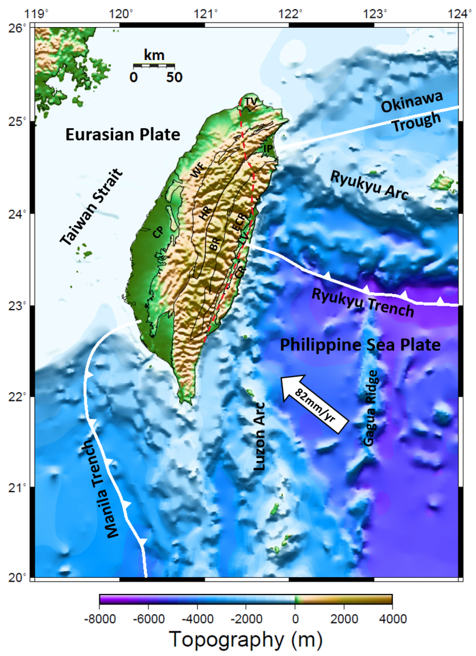
Taiwan is located at the collision zone between the Eurasian Plate and the Philippine Sea Plate. GPS observations show that the crust of Taiwan continues to rise vertically due to the compression of plates [1]. In the southeast part of Taiwan, the Philippine Sea Plate is squeezed towards the Eurasian Plate at a speed of 82 mm/year [2]. In the northeast part of Taiwan, the Philippine Sea Plate has been subducting under the Eurasian Plate along the Ryukyu Trench. The plate configuration in the vicinity of Taiwan is shown in Figure 1. The distribution of earthquake hypocenters forms a sloping northwest subduction zone. However, the Eurasian Plate subducts eastward under the Philippine Sea Plate at the southern part of Taiwan [3], which results in the active orogeny process in Taiwan. The collision not only causes a series of folds and faults but also induces frequent earthquakes around Taiwan area. Many models have been proposed to explain the orogeny process around Taiwan area due to the collision of the Eurasian Plate and the Philippine Sea Plate. Some examples are as follows: the thin-skin model advocates that the orogenic movement is only carried out above the detachment surface [4]; the lithospheric collision model indicates that the whole lithosphere is deformed and forms mountain roots [5]; a model of breaking the Eurasian Plate beneath Taiwan can show the reversal of the subduction polarity in northern Taiwan [6]; a model of active continental subduction followed by crustal exhumation [7]; a subducting indenter model using seismicity and 3D velocity structures [8].
In recent years, with the widespread establishment of broadband seismic stations in Taiwan, abundant seismic data have become available for the study of Taiwan’s geological structure. One important achievement is using seismic tomography to estimate the velocity structure beneath Taiwan by utilizing these high-quality seismic broadband data [9,10,11,12,13]. However, velocity tomography can exhibit structures with different velocities, but fails to distinguish structures with no velocity difference. Moreover, the Moho velocity under Taiwan has not yet been determined with confidence; thus, it is still difficult to judge the position and depth of the Moho from the velocity model.
When the teleseismic P-wave passes through an interface between two materials with different acoustic impedances, the P-wave and the converted S-wave are transmitted out from the interface. Thus, the depth of the interface can be estimated by the difference in travel time between the P-wave and converted S-wave. The receiver function method was first proposed by Phinney [14], which is the deconvolution of the incoming vertical and longitudinal components of the seismogram; thus, it contains the information of the time difference between the P-wave and converted S-wave. Therefore, the interface (for example, Moho discontinuity) of two materials (for example, crust and mantle) with different acoustic impedances can be estimated by the receiver function. Then, this method was refined by Langston [15], who converted the receiver function spectrum back to the time domain and used the “water-level” technique to stabilize the deconvolution result, and then used a Gaussian function low-pass filter to reduce the high-frequency noise. Owens et al. [16] developed an iterative linearized inversion procedure in the time domain to obtain a one-dimensional velocity model. Ammon [17] discovered that the receiver function is sensitive to the relative velocity of the crust rather than the absolute velocity. Therefore, the difference in impedance of the medium is the main factor in producing a clear receiver function. Ammon [18] proposed that the absolute amplitude of the receiver function is affected by the angle of incidence and the refractive index, and the amplitude will decrease with the increase of the epicenter distance. Nowadays, this is the common method used to study the structure of the crust and upper mantle [19,20,21,22,23]. In addition, Zhu [21] developed the Common Conversion Point (CCP) stacking technique by stacking the conversion positions so the position of the crustal structure can be imaged more clearly.
Thereafter, the single-station receiver function was used to explore the crustal structure of Taiwan [10, 24,25,26]. Thus, the Moho depths under the stations can be demonstrated but the Moho depths between stations are still unknown. From 2007 to 2009, high-quality seismic data were acquired by two high-density linear arrays deployed at north Taiwan in east–west and south–north directions, which are part of the TAiwan Integrated GEodynamics Research (TAIGER) project. These high-density array data and the receiver function method incorporating the CCP stacking technique [21] are used to image the crustal structure beneath northern Taiwan in this study. In the following sections, the origin of the seismic data and the methodology of receiver function are given. Then, the CCP stack of receiver functions of the two high-density linear arrays are calculated and interpreted, and finally, the discussions and conclusions of the receiver functions beneath northern Taiwan are demonstrated.
2. Seismic Data
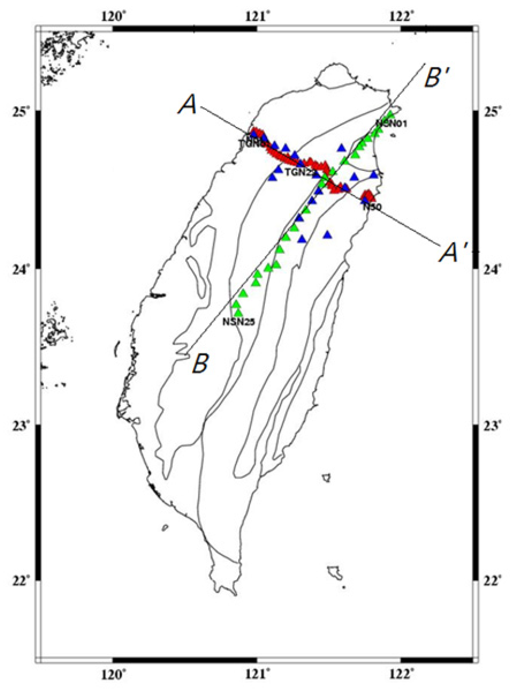
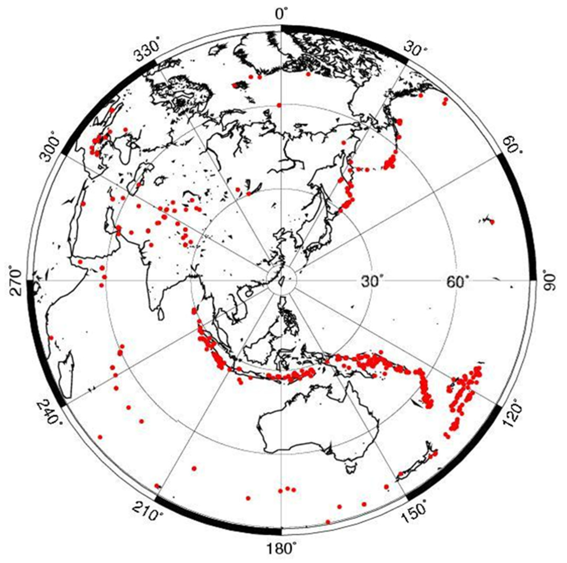
The TAIGER project deployed two high-density linear seismic arrays in north Taiwan. The first is composed of 19 broadband (Guralp CMG-3T, 120 s) seismic stations installed from May 2007 to July 2008 and 45 short-period (Sercel L-22, 2 Hz) seismic stations installed from March 2008 to June 2008 in the east–west direction, which are shown in Figure 2 as blue and red triangles, respectively. The other is composed of 25 broadband (Nanometrics Trillium 120, 120 s and Guralp CMG-3ESP, 120 s) stations installed from February 2008 to June 2009 in the south–north direction, shown as green triangles in Figure 2. Although there are two types of instruments used in this study, the instrument and source effects were removed, leaving only the path effect, by deconvolution of the radial component with the vertical component of the teleseismic P-wave in obtaining the receiver function. Thus, the broadband and short-period receiver functions can be used in combination. Since the influence and bias induced by the variation in the lateral crustal structural on the CCP stacking can be reduced by the full azimuthal coverage of the teleseismic earthquakes, the full back-azimuth coverage of the teleseismic earthquakes for performing the receiver function and CCP stacking is required. The teleseismic earthquakes are sorted during the array operation time for those whose magnitudes (Mw) are greater than 5.0 and the epicenter distances are between 30° and 90° with full back-azimuth coverage from the two arrays. There are 388 teleseismic earthquakes fitted the requirements, shown in Figure 3. In total, there were 2833 direct P-wave events detected in the two arrays for these 388 teleseismic earthquakes. Data quality is crucial in the receiver function analysis. Therefore, the poor signal-to-noise ratio data and harmful traces are removed. Finally, there are 1211 and 1287 events are used in the east–west and south–north profiles, respectively.
3. Methods of Receiver Function and CCP Stacking
3.1. Receiver Function
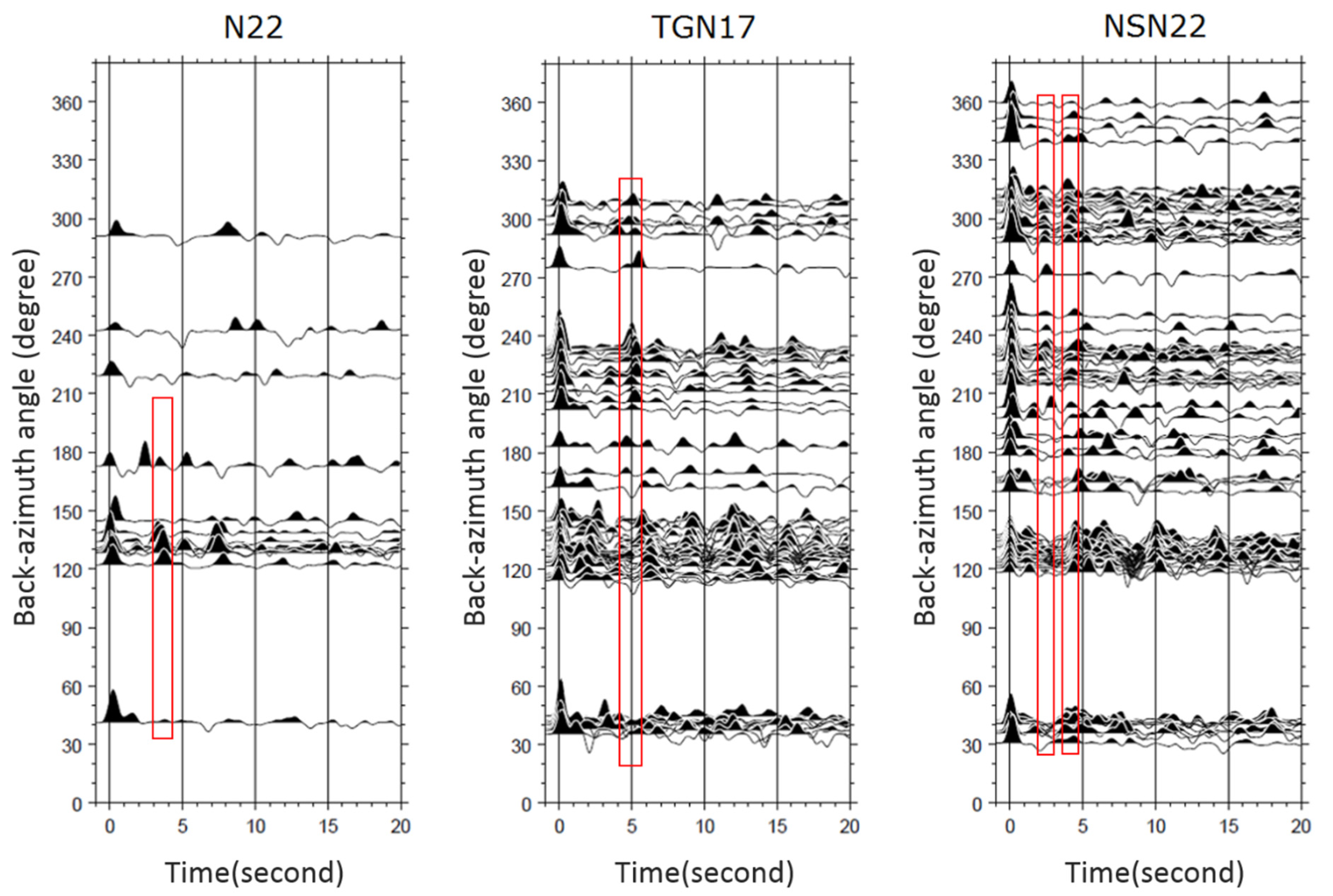
The receiver function method refined by Langston [27] and Owens et al. [16] shows that the source and instrument effects can be removed using the division of the radial component by the vertical component of the teleseismic P-wave operated in the frequency domain. The corresponding time sequence of the divide is called the receiver function, which contains the converted phase produced by the interface beneath the receiver. Thus, the receiver function can be used to indicate the depth of the interface. The teleseismic P-waves used in this study were first filtered by a Butterworth filter from 0.1 to 2.0 Hz. Then, all first arriving P-waves of the vertical components were aligned by the waveform cross-correlation technique. Next, the receiver functions were calculated using the time-domain iterative deconvolution technique [28]. Finally, the receiver functions were filtered by the Gaussian low-pass filter (1 Hz) to suppress the high-frequency noises for imaging. Figure 4 shows the receiver functions of the teleseismic P-wave detected by stations N22, TGN17 and NSN22. Stations N22 and TGN17 are the short-period and broadband seismic stations distributed at the same position in the AA′ profile but at a different time period. The 3-s events appearing in stations N22 and TGN17 are consistent. However, the 5-s events only appear in station TGN17, since long travel time events are more easily detected by the broadband seismic station. NSN22 is the broadband seismic station deployed in BB′ profile. The 3- and 4-s events can be seen in the station NSN22 during the azimuth angles of 200–360 degrees. When compared with previously mentioned studies [20,21,23], the events appearing in these back-azimuth receiver function plots are random, which shows that the structure below Taiwan is complex. This also indicates the importance of using array data to refocus individual events to their originated places.
3.2. CCP Stacking (Common Conversion Point Stacking)
In this study, the CCP stacking technique [21] was used to image the crustal structure. Since the amplitude of the time sequence of receiver function represents the acoustic impedance change of the medium at the conversion point, the amplitude at each point on the receiver function is assigned to the corresponding position on the ray path, where the P-S conversion occurs for the time relative to the direct P-wave. Then, the study area along the profile is gridded into sufficiently small pixels, and all amplitudes in each pixel are summed to obtain the average amplitude. Therefore, the image of the crustal structure along the profile is obtained. A background velocity model modified from the velocity model of Wu et al. [12] was used to calculate the ray path of the receiver function, and then, we applied the CCP stacking technique to stack all the receiver functions of teleseismic events along the profile. Then, the CCP stacking image was obtained along the profile.
4. Imaging results
4.1. A-A′ Profile
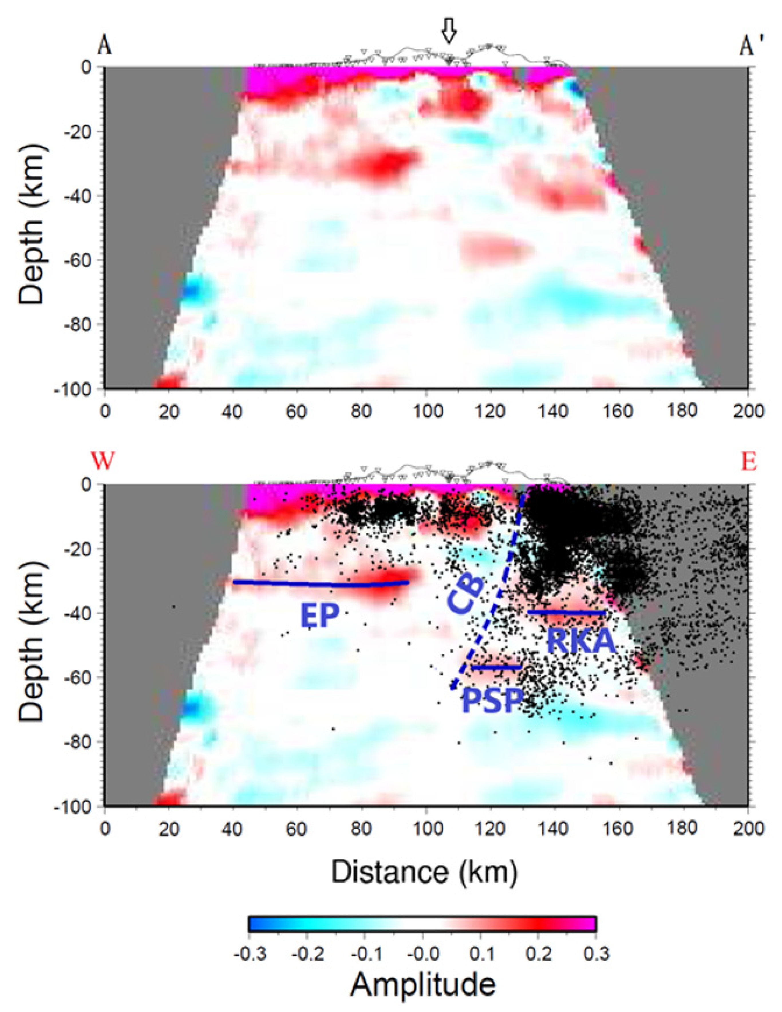
The seismic data acquired by the east–west high-density linear seismic array were processed by the receiver function and CCP stacking methods and then projected to the A-A′ profile, shown in Figure 5. The topography of Taiwan along the A-A′ profile is shown at the top of the figure. The triangles represent the locations of seismic stations which are projected to the A-A′ profile and the arrow indicates the cross point of profiles A-A′ and B-B′, where the latitude and longitude are 24.6 degrees N and 121.5 degrees E. The top figure is the CCP stack of receiver functions along the profile. The bottom figure is the interpretation of the top figure and incorporated with the earthquakes relocated by Wu et al. [29] for magnitude (ML) ≥ 3.0 in the past 15 years. A collision boundary could be seen from the distribution of earthquakes and the CCP stack of receiver functions, shown by the blue dashed line and characters “CB” in the figure. The surface position of the boundary is at 121.7 degrees E longitude. On the west side of this boundary, most of the earthquake depths are shallower than 20 km. However, on the east of the boundary, the earthquake depths are relatively deep. The deepest depth of the earthquakes is about 60 km. Thus, this boundary could be the collision boundary between the Eurasian Plate and the Philippine Sea Plate. The west part of the boundary is the Eurasian Plate and the east part is the Philippine Sea Plate and the Ryukyu arc. This collision position is consistent with the plate boundary between the Eurasian Plate and Philippine Sea Plate of Wu et al. [8]. A strong horizontal event appeared at a depth of 30 km and horizontal distances of 30–90 km, shown by a blue line and characters “EP”, which is interpreted as the Moho discontinuity of the Eurasian Plate. This indicates that the Moho of the Eurasian Plate is flat, its depth is 30 km in the north-west of Taiwan. In addition, the event for the horizontal distances of 110–130 km at a depth of 55 km shown by a blue line and characters “PSP” is considered as the Moho discontinuity of the Philippine Sea Plate. Since this area is just below the cross point of profiles A-A′ and B-B′, this interpretation is supported by the B-B′ profile (Figure 6). The event for the horizontal distances of 130–160 km at a depth of 40 km, shown by a blue line and characters “RKA”, is considered as the Moho discontinuity of the Ryukyu arc. This indicates that the crust of the Ryukyu arc was deposited on the Philippine Sea Plate and pushed into the Eurasian Plate.
4.2. B-B′ Profile
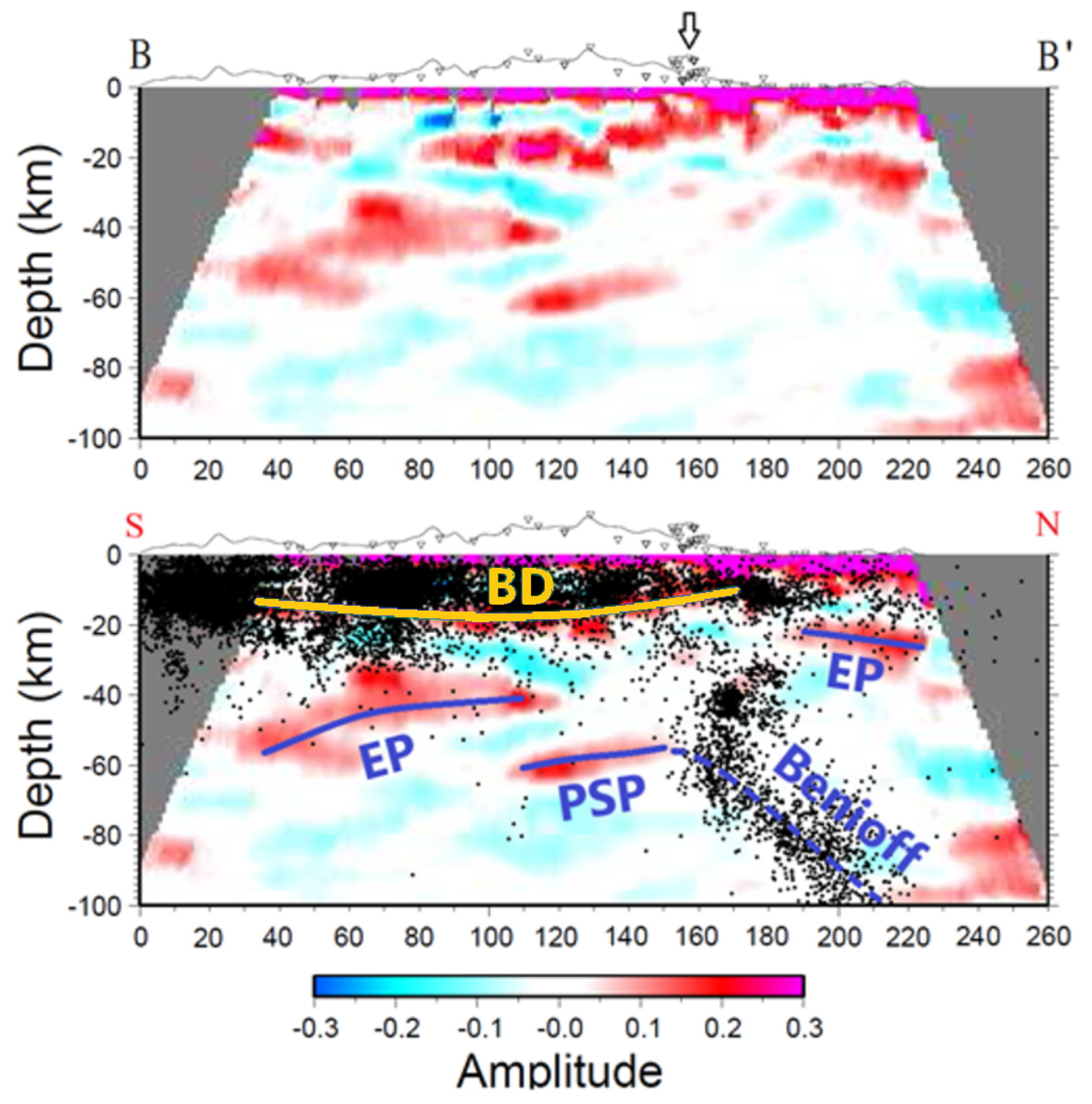
The seismic data acquired from the south–north high-density linear seismic array were processed by the same techniques used in profile A-A′ and then projected to the B-B′ profile, shown in Figure 6. The topography along the B-B′ profile is shown at the top of the figure. The top figure is the CCP stack of receiver functions and the bottom figure is the interpretation of the top figure incorporated with the earthquakes relocated by Wu et al. [29] for magnitude (ML) ≥ 3.0 in the past 15 years. An interface is seen at depths of 15–20 km and horizontal distances of 40–180 km, shown by a yellow line and characters “BD”. Almost all of the earthquakes occur above this interface, which is considered as a brittle–ductile transition zone in the upper crust. This position is consistent with the study results of crustal rheology in Taiwan by Kidder et al. [30] based on the analysis of the composition and deformation of quartzite. This upper crustal structure is similar to those in the Baltic Shield, where there is an interface in the upper crustal and almost all earthquakes occur above this interface [31]. However, almost all of the stations distributed in the A-A′ profile are on the alluvial plain, and the multi-reflection waves induced in the low-velocity sedimentary layers contaminate the shallow structure signals; therefore, the brittle–ductile transition zone is not found in the A-A′ profile. On the contrary, the stations deployed in the B-B′ profile are on the rock site, thus no multi-reflection wave is produced here and the brittle–ductile transition zone is observed in the B-B′ profile.
In the northmost part of the profile, a strong event appeared at depths of 20–25 km and horizontal distances of 180–220 km, shown by the blue line and characters “EP”, which is interpreted as the Moho discontinuity of the Eurasian Plate. In addition, the event for horizontal distances of 110–150 km at depths of 55–60 km, shown by the blue line and characters “PSP”, is considered as the Moho discontinuity of the Philippine Sea Plate. Wu et al. [8] showed that the western edge of the Philippine Sea Plate is inserted into the asthenosphere at a depth of 50 km below the Eurasian Plate in northern Taiwan. The depth and position of the western edge of the Philippine Sea Plate are consistent with our results. There are two groups of earthquakes for horizontal distances of 160–200 km in this profile. One group, at depths of 20–60 km and located at the plate boundary, is considered as the collision zone of the Eurasian Plate and the Philippine Sea Plate. Another group dips northward at depths of 60–100 km, shown by the blue dashed line and word “Benioff”, which is regarded as the Benioff seismic zone. This indicates that the Philippine Sea Plate is subducting northward under the Eurasian Plate along the Ryukyu Trench in north Taiwan. This interpretation is consistent with those proposed by Kao and Rau [32]. In addition, the event for horizontal distances of 40–110 km, shown by the blue line and characters “EP”, is considered as the Moho discontinuity of the Eurasian Plate at depths of 40–55 km. Overall, the depth of the Moho discontinuity of the Eurasian Plate gradually becomes deeper from north Taiwan to the center of Taiwan. The deepest Moho discontinuity is the Philippine Sea Plate at the center of Taiwan, with a depth of 60 km.
5. Discussions
The seismic tomogram can show the crustal velocity structure, and the receiver function responds to the crustal impedance structure, although the physical meanings of the velocity and impedance are different but similar. Thus, they can be compared with each other. Rau and Wu [10] used the P-wave arrival times of local earthquakes to inverse (or tomography) the P-wave velocity structures around Taiwan region, which shows that the crust is thick under the Central Mountain Range and thinner at the Western Foothills region than in other areas. The tomographic results of Kim et al. [11], indicate that the Moho depth is about 35 km beneath the Coastal Plain at western Taiwan and increases rapidly toward the east and reaches its maximum depth of 55 km beneath the eastern Central Mountain Range. Wu et al. [12] used the P- and S-wave arrival times of local earthquakes and the time differences between the arrival times of S- and P-waves from a dense network of strong motion stations (Taiwan Strong Motion Instrumentation Program network) to image the Vp and Vp/Vs structures beneath Taiwan. Their seismic tomogram shows that the Moho depth is about 60 km under the Central Mountain Range. Ustaszewski et al. [33] used the velocity tomography and seismic distribution to map the crust–mantle boundaries, showing that the Philippine Sea Plate subsides to the north and dips eastward under the Eurasian Plate, and the western edge of the Philippine Sea plate at 24.2 degrees N latitude is about 50–60 km in depth and the depth variation is gentle. This is consistent with “PSP” in the BB′ profile. Li et al. [34] used the joint inversion of P- and S-wave arrival times and Bouguer gravity to estimate the 3D velocity structures around the Taiwan area. Their study shows the maximum Moho depth is 56 km and located beneath the Backbone Range (or Western Central Mountain Range), and the trend of the Moho is largely consistent with the topography of the Central Mountain Range. To summarize the comparison with the seismic tomogram, the Moho depths around northern Taiwan estimated by the seismic tomograms are consistent with our results.
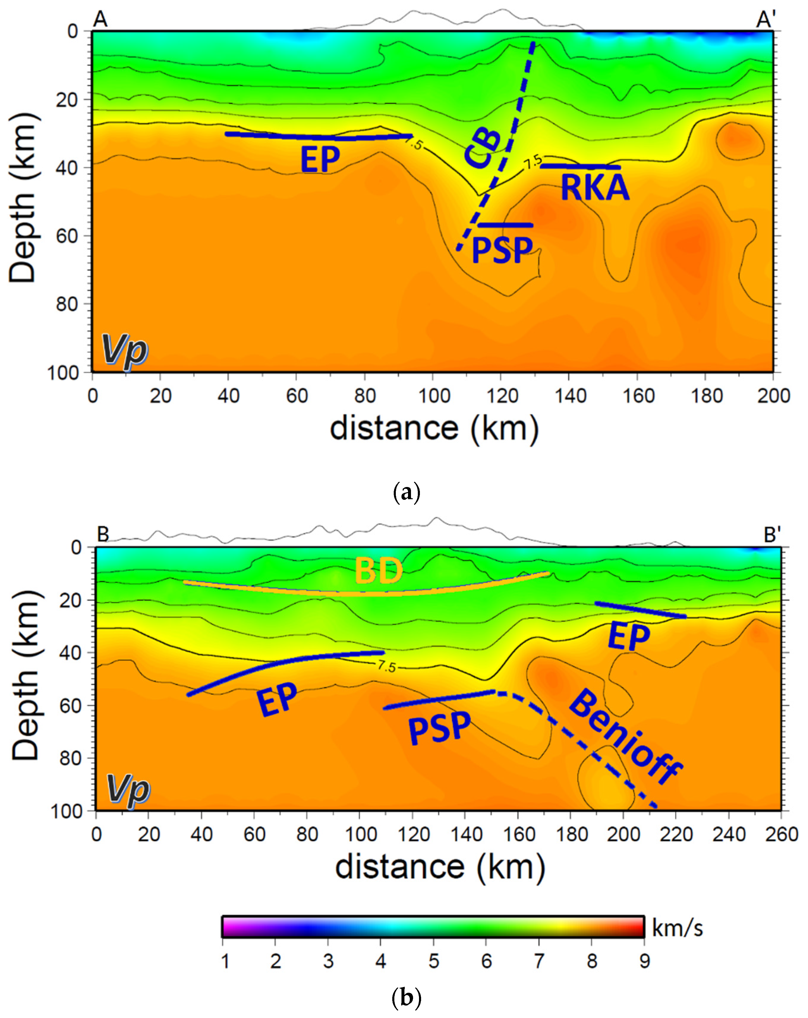
The tomographic P-wave velocity model around the Taiwan region built by Kuo-Chen et al. [13] is used for a comparison with our results. Their P-wave velocity model along the A-A′ and B-B′ profiles are shown in Figure 7a,b, respectively. Using the 7.5 km/s contour as the bottom of the crust [13], and the interval of the contour lines being 0.5 km/s, “two parallel roots” beneath Taiwan were found in their study, which can be seen in the east–west direction velocity profile (Figure 7a). The main root is under the Central Mountain Range and its depth is 50 km, corresponding with the “PSP” for horizontal distances of 110–130 km in Figure 5. The other root is under the Coastal Range and its depth is 40 km, corresponding with the “RKA” for horizontal distances of 130–160 km in Figure 5. In the west side of Figure 7a, the crust depth is nearly horizontal at depths of 28–30 km, correspondent with the “EP” for horizontal distances of 30–90 km in Figure 5. To compare the B-B′ profile (Figure 6) with south–north direction velocity profile (Figure 7b) from south to north; the depth of the crust is about 40 km for the horizontal distances of 40–110 km, the deepest part of the crust is about 45–50 km for the horizontal distances of 120–160 km and shallowest part of the crust is about 25–30 km for the horizontal distances of 190–240 km in Figure 7b, which are correlated with south “EP”, “PSP” and north “EP” in Figure 6, respectively. Although there are little differences in depth between our interpretations and Kuo-Chen et al.‘s Moho depths, the overall trends are consistent. The CCP stack image clearly indicates the positions of the interfaces. In addition, Figure 7 also indicates that the geological structures are very complex in northern Taiwan, which are induced by the collision of the Eurasian Plate and the Philippine Sea Plate. The complexity of geological structures captured by seismic waves can be quantitatively assessed by the seismic propagators [35], so the optimum solution can be estimated by a compromise between geological complexity, seismic imaging accuracy, and computational efficiency.
In the following, more comparisons of using receiver function to study the crustal structure of Taiwan are made. Tomfohrde and Nowack [24] used receiver function and Taiwan Seismographic Network data to inverse the one-dimensional velocity model under each station. Their results show that the average Moho depth is 38 km surrounding the Central Mountain Range of Taiwan. Kim et al. [25] analyzed the teleseismic receiver function of each BATS (Broadband Array in Taiwan for Seismology) station and found that the crustal thicknesses are 20–30 km at the TWB1 station and 44–46 km at the SSLB station. The TWB1 and SSLB stations are close to the horizontal distances of 220 and 60 km of the B-B′ profile. Wang et al. [26] used the H-κ stacking method proposed by Zhu and Kanamori [36] to estimate crustal thickness and Vp/Vs ratio for each BATS station in Taiwan. Their results show that the Moho depth is shallow (17–32 km) in northern and southeastern Taiwan, becomes deep (32–39 km) in southwestern, and the deepest depth is about 53 km below the SSLB station in central Taiwan. Goyal and Hung [37] applied the H-V stacking method [38] which jointly utilized P- and S-wave receiver functions to determine the Moho depths beneath the 50 stations in Taiwan and off-shore islands. Their results show that the Moho depth is about 20 km in the north and west coastal areas of Taiwan. The Moho depth deepens from coastal areas to the Central Mountain Range, and the maximum depth below the midwest of the Central Mountain Range is about 47 km. Their overall depth of the Moho is 10 km shallower than ours, but the position and trend of the variation in Moho depth are consistent with ours. The above-mentioned study results are consistent with ours. However, our results show the continuous variation of the Moho depth beneath northern Taiwan.
For comparison with the density structure, Hsieh and Yen [39] used 3D gravity inversion to estimate the density structure of Taiwan and showed that the Moho depth in the west of Taiwan is 30–35 km, corresponding to the “EP” in the AA′ profile. Their maximum Moho depth is 45–50 km beneath the middle Central Mountain Range, which is shallower than our result, but the position is similar.
The thin-skin model asserts that there is a detachment surface near the subduction plate boundary, and all orogeny processes could only be carried out above the detachment surface. The detachment surface slopes eastward and is about 5–15 km in depth below Taiwan [40]. However, the lithospheric collision model is opposed to the statement of the detachment surface. According to the 1–2 s delay in the teleseismic shear wave, the plates uplift and extend downwards to form roots under the arc-continent collision [5]. Based on our results, taking the collision of the Eurasian Plate and the Philippine Sea Plate as the boundary, the west of the boundary is consistent with the thin-skin model, where the Eurasian crust is thin and flat. In addition, the east of the boundary is similar to the lithospheric collision model, where the lithosphere of the Philippine Sea Plate is deformed and forms the mountain root.
Kind et al. [41] showed that CCP stacking would be unable to image an oblique plate with a dip of more than 30 degrees, since the converted S-wave might destructively interfere in CCP stacks. The same result is observed in our results, that oblique plates with a dip of more than 30 degrees cannot be imaged in the CCP stacks. Although this limit restricts the capability of the CCP stack of receiver functions, most of the near-horizontal Moho discontinuities could still be imaged clearly. In addition, the velocity model used in the CCP stack of receiver functions would affect the depths of the interfaces; a 10% change in the velocity model yields a 5–10% change in the depth of the Moho [42]. Thus, the absolute depth of the Moho interface may have some error; the relative depth relationship of the Moho interfaces is still true. In addition, the Moho interfaces can be delineated in the image so that their horizontal variations can be easily observed.
6. Conclusions
The crustal structure beneath northern Taiwan has been studied using receiver function and CCP stacking methods with data of two dense linear seismic arrays. As a result, in the A-A′ profile (east–west direction), a collision boundary between the Philippine Sea Plate and the Eurasian Plate is observed in the east of Taiwan (121.7 degrees E longitude). The Moho discontinuity of the Eurasian Plate in the west of northern Taiwan is flat, and its depth is 30 km. The depth of the Moho below the Central Mountain Range, which belongs to the Philippine Sea Plate, is about 55 km. The depth of the Moho in the east, which belongs to the crust of the Ryukyu arc, is about 40 km. In the B-B′ profile (south–north direction), a brittle–ductile transition zone at depths of 15–20 km beneath central Taiwan from south to north is found. The Moho depth of the Eurasian Plate is about 20–25 km in northern Taiwan. The Moho depth of the Eurasian Plate becomes gradually deeper, from 40 to 55 km from north to south in central Taiwan. The deepest Moho, the Philippine Sea Plate, which is located at the junction of the two profile lines (24.6 degrees N latitude and 121.5 degrees E longitude), has a depth of 60 km. According to these results, the crustal structure in the west of the collision boundary between the Philippine Sea Plate and the Eurasian Plate is consistent with the thin-skin model, where the Eurasian Plate is thin and flat; the crustal structure in the east part of the collision boundary is similar to the lithospheric collision model, where the lithosphere of the Philippine Sea Plate is deformed and to form the mountain root.
Author Contributions
Conceptualization, T.-C.C. and B.-S.H.; methodology, T.-C.C.; formal analysis, T.-C.C.; investigation, T.-C.C. and Y.-F.C.; data curation, T.-C.C.; writing—original draft preparation, T.-C.C.; writing—review and editing, Y.-F.C.; supervision, Y.-F.C.; funding acquisition, Y.-F.C. All authors have read and agreed to the published version of the manuscript.
Funding
This work is partially funded under the Ministry of Science and Technology grant 110-2116-M-194-014.
Data Availability Statement
Not applicable.
Acknowledgments
The authors gratefully thank Lupei Zhu for kindly providing his software package of the receiver function. We also gratefully thank the journal editor and the two reviewers for their valuable insights and recommendations for improving this manuscript.
Conflicts of Interest
The authors declare no conflict of interest.
References
- Ching, K.E.; Rau, R.J.; Johnson, K.M.; Lee, J.C.; Hu, J.C. Present-day kinematics of active mountain building in Taiwan from GPS observations during 1995–2005. J. Geophys. Res. 2011, 116, B09405. [Google Scholar] [CrossRef]
- Yu, S.B.; Chen, H.Y.; Kuo, L.C. Velocity field of GPS stations in the Taiwan area. Tectonophysics 1997, 274, 41–59. [Google Scholar] [CrossRef]
- Tsai, Y.B.; Teng, T.L.; Chiu, J.M.; Liu, H.L. Tectonic implications of the seismicity in the Taiwan region. Mem. Geol. Soc. China 1977, 2, 13–41. [Google Scholar]
- Suppe, J. Mechanics of mountain building and metamorphism in Taiwan. Mem. Geol. Soc. China 1981, 4, 67–89. [Google Scholar]
- Wu, F.T.; Rau, R.J.; Salzberg, D. Taiwan orogeny: Thin-skinned or lithospheric collision? Tectonophysics 1997, 274, 191–220. [Google Scholar] [CrossRef]
- Teng, L.S.; Lee, C.T.; Tsai, Y.B.; Hsiao, L.Y. Slab breakoff as a mechanism for flipping of subduction polarity in Taiwan. Geology 2000, 28, 155–158. [Google Scholar] [CrossRef]
- Lin, C.H. Active continental subduction and crustal exhumation: The Taiwan orogeny. Terra Nova 2002, 14, 281–287. [Google Scholar] [CrossRef] [Green Version]
- Wu, F.T.; Liang, W.T.; Lee, J.C.; Benz, H.; Villasenor, A. A model for the termination of the Ryukyu subduction zone against Taiwan: A junction of collision, subduction/separation, and subduction boundaries. J. Geophys. Res. 2009, 114, B07404. [Google Scholar] [CrossRef] [Green Version]
- Roecker, S.W.; Yeh, Y.H.; Tsai, Y.B. Three-dimensional P and S wave velocity structures beneath Taiwan; deep structure beneath an arc-continent collision. J. Geophys. Res. 1987, 92, 10547–10570. [Google Scholar] [CrossRef]
- Rau, R.J.; Wu, F.T. Tomographic imaging of lithospheric structures under Taiwan. Earth Planet. Sci. Lett. 1995, 133, 517–532. [Google Scholar] [CrossRef]
- Kim, K.H.; Chiu, J.M.; Pujol, J.; Chen, K.C.; Huang, B.S.; Yeh, Y.H.; Shen, P. Three-dimensional Vp and Vs structural model associated with the active subduction and collision tectonics in the Taiwan region. Geophys. J. Int. 2005, 162, 204–220. [Google Scholar] [CrossRef] [Green Version]
- Wu, Y.M.; Chang, C.H.; Zhao, L.; Shyu, J.B.H.; Chen, Y.G.; Sieh, K.; Avouac, J.P. Seismic tomography of Taiwan: Improved constraints from a dense network of strong motion stations. J. Geophys. Res. 2007, 112, B08312. [Google Scholar] [CrossRef]
- Kuo-Chen, H.; Wu, F.T.; Roecker, S.W. Three-dimensional P velocity structures of the lithosphere beneath Taiwan from the analysis of TAIGER and related seismic data sets. J. Geophys. Res. 2012, 117, B06306. [Google Scholar] [CrossRef] [Green Version]
- Phinney, R.A. Structure of the Earth’s crust from spectral behavior of long-period body waves. J. Geophys. Res. 1964, 62, 2997–3017. [Google Scholar] [CrossRef]
- Langston, C.A. Structure under Mount Rainier, Washington, inferred from teleseismic body waves. J. Geophys. Res. 1979, 84, 4749–4762. [Google Scholar] [CrossRef] [Green Version]
- Owens, T.J.; Zant, G.; Taylor, S.R. Seismic evidence for an ancient rift beneath the Crumberland Plateau, Tennessee: A Detailed analysis of broadband teleseismic P waveforms. J. Geophys. Res. 1984, 89, 7783–7795. [Google Scholar] [CrossRef]
- Ammon, C.J.; Randall, G.E.; Zandt, G. On the nonuniqueness of receiver function inversions. J. Geophys. Res. 1990, 95, 15303–15318. [Google Scholar] [CrossRef]
- Ammon, C.J. The isolation of receiver effects from teleseismic P waveforms. Bull. Seismol. Soc. Am. 1991, 81, 2504–2510. [Google Scholar] [CrossRef]
- Peng, X.; Humphreys, E.D. Crustal velocity structure across the eastern Snake River Plain and Yellowstone swell. J. Geophys. Res. 1998, 103, 7171–7186. [Google Scholar] [CrossRef] [Green Version]
- Xu, L.; Rondenay, S.; van der Hilst, R.D. Structure of the crust beneath the southeastern Tibetan Plateau from teleseismic receiver functions. Phys. Earth Planet. Inter. 2007, 165, 176–193. [Google Scholar] [CrossRef]
- Zhu, L. Crustal structure across the San Andreas Fault, southern California from teleseismic converted waves. Earth Planet. Sci. Lett. 2000, 179, 183–190. [Google Scholar] [CrossRef]
- Farra, V.; Vinnik, L. Upper mantle stratification by P and S receiver functions. Geophys. J. Int. 2000, 141, 699–712. [Google Scholar] [CrossRef]
- Chen, Y.; Niu, F.; Liu, R.; Huang, Z.; Tkalčić, H.; Sun, L.; Chan, W. Crustal structure beneath China from receiver function analysis. J. Geophys. Res. 2010, 115, B03307. [Google Scholar] [CrossRef] [Green Version]
- Tomfohrde, D.A.; Nowack, R.L. Crustal structure beneath Taiwan using frequency-band inversion of receiver function waveforms. Pure Appl. Geophys. 2000, 157, 737–764. [Google Scholar] [CrossRef] [Green Version]
- Kim, K.H.; Chiu, J.M.; Kao, H.; Liu, Q.; Yeh, Y.H. A preliminary study of crustal structure in Taiwan area using receiver function analysis. Geophys. J. Int. 2004, 159, 146–164. [Google Scholar] [CrossRef] [Green Version]
- Wang, H.L.; Zhu, L.; Chen, H.W. Moho depth variation in Taiwan from teleseismic receiver functions. J. Asian Earth Sci. 2010, 37, 286–291. [Google Scholar] [CrossRef]
- Langston, C.A. The effect of planar dipping structure on source and receiver responses for constant ray parameter. Bull. Seismol. Soc. Am. 1977, 67, 1029–1050. [Google Scholar]
- Ligorría, J.P.; Ammon, C.J. Iterative deconvolution and receiver-function estimation. Seismol. Soc. Am. 1999, 89, 1395–1400. [Google Scholar] [CrossRef]
- Wu, Y.M.; Chang, C.H.; Zhao, L.; Teng, T.L.; Nakamura, M. A comprehensive relocation of earthquakes in Taiwan from 1991 to 2005. Bull. Seismol. Soc. Am. 2008, 98, 1471–1481. [Google Scholar] [CrossRef] [Green Version]
- Kidder, S.; Avouac, J.P.; Chan, Y.C. Constraints from rocks in the Taiwan orogen on crustal stress levels and rheology. J. Geophys. Res. 2012, 117, B09408. [Google Scholar] [CrossRef]
- Korhonen, H.; Porkka, M.T. The structure of the baltic shield region on the basis of DSS and earthquake data. Pure Appl. Geophys. 1981, 119, 1093–1099. [Google Scholar] [CrossRef]
- Kao, H.; Rau, R.J. Detailed structures of the subducted Philippine Sea plate beneath northeast Taiwan: A new type of double seismic zone. J. Geophys. Res. 1999, 104, 1015–1033. [Google Scholar] [CrossRef] [Green Version]
- Ustaszewski, K.; Wu, Y.M.; Suppe, J.; Huang, H.H.; Chang, C.H.; Carena, S. Crust-Mantle boundaries in the Taiwan-Luzon arc-continent collision system determined from local earthquake tomography and 1D models: Implications for the mode of subduction polarity reversal. Tectonophysics 2012, 578, 31–49. [Google Scholar] [CrossRef]
- Li, Z.; Roecker, S.; Kim, K.; Xu, Y.; Hao, T. Moho depth variations in the Taiwan orogen from joint inversion of seismic arrival time and Bouguer gravity data. Tectonophysics 2014, 632, 151–159. [Google Scholar] [CrossRef]
- Fu, L. Quantitative assessment of the complexity of geological structures in terms of seismic propagators. Sci. China. Earth Sci. 2010, 53, 54–63. [Google Scholar] [CrossRef]
- Zhu, L.; Kanamori, H. Moho depth variation in southern California from teleseismic receiver functions. J. Geophys. Res. 2000, 105, 2890–2969. [Google Scholar] [CrossRef] [Green Version]
- Goyal, A.; Hung, S.H. Lateral variations of Moho depth and average crustal properties across the Taiwan orogen from H-V stacking of P and S receiver functions. Geochem. Geophys. Geosyst. 2021, 22, e2020GC009527. [Google Scholar] [CrossRef]
- Rychert, C.A.; Harmon, N. Stacked P-to-S and S-to-P receiver functions determination of crustal thickness, Vp, and Vs: The H-V stacking method. Geophys. Res. Lett. 2016, 43, 1487–1494. [Google Scholar] [CrossRef] [Green Version]
- Hsieh, H.H.; Yen, H.Y. Three-dimensional density structures of Taiwan and tectonic implications based on the analysis of gravity data. J. Asian Earth Sci. 2016, 124, 247–259. [Google Scholar] [CrossRef]
- Carena, S.; Suppe, J.; Kao, H. Active detachment of Taiwan illuminated by small earthquakes and its control of first-order topography. Geology 2002, 30, 935–938. [Google Scholar] [CrossRef]
- Kind, R.; Eken, T.; Tilmann, F.; Sodoudi, F.; Taymaz, T.; Bulut, F.; Yuan, X.; Can, B.; Schneider, F. Thickness of the lithosphere beneath Turkey and surroundings from S-receiver functions. Solid Earth 2015, 6, 971–984. [Google Scholar] [CrossRef] [Green Version]
- Caldwell, W.B.; Klemperer, S.L.; Lawrence, J.F.; Rai, S.S.; Ashish. Characterizing the Main Himalayan thrust in the Garhwal Himalaya, India, with receiver function CCP stacking. Earth Planet. Sci. Lett. 2013, 367, 15–27. [Google Scholar] [CrossRef]
Figure 1.
Plate configuration in the vicinity of Taiwan. The Philippine Sea Plate is moving northwestward with a rate of 82 mm/year and colliding with the Eurasian Plate. The red dotted line is the western edge of the Philippine Sea Plate, which is modified from Wu et al. [8]. IP = Ilan Plain, TV = Tatun volcano, LV = Longitudinal Valley, CP = Coastal Plain, HR = Hsueshan Range, WF = Western Foothills, BR = Backbone Range (or Western Central Mountain Range), ECR = Eastern Central Mountain Range and CR = Coastal Range.

Figure 2.
The positions of two orthogonal linear dense arrays deployed in north Taiwan in east–west (A-A′ line) and south–north (B-B′ line) directions. The blue triangles represent 19 broadband seismic stations installed from May 2007 to July 2008. The green triangles indicate 25 broadband stations installed from February 2008 to June 2009, and the red triangles are 45 short-period stations installed from March 2008 to June 2008.

Figure 3.
The red dots are the positions of the epicenters of the teleseismic earthquakes used in this study, in which the magnitudes are larger than 5.0 Mw and the epicenter distances are between 30° and 90°.
Figure 3.
The red dots are the positions of the epicenters of the teleseismic earthquakes used in this study, in which the magnitudes are larger than 5.0 Mw and the epicenter distances are between 30° and 90°.

Figure 4.
Back-azimuth receiver function plots of stations N22, TGN17 and NSN22.

Figure 5.
The CCP stack of receiver functions along the A-A′ profile. The topography along the A-A′ profile is shown at the top of the figure. The triangles represent the locations of seismic stations which are projected to the A-A′ profile and the arrow indicates the cross point of profiles A-A′ and B-B′. The top figure is the CCP stack of receiver functions along the profile. The bottom figure is the interpretation of the top figure and incorporated with the earthquakes relocated by Wu et al. [29] for magnitude (ML) ≥ 3.0 in the past 15 years. The blue dashed line represents the collision boundary “CB” between the Philippine Sea Plate and the Eurasian Plate. The blue lines indicate the Moho discontinuities of the Eurasian Plate (EP), Philippine Sea Plate (PSP) and Ryukyu arc (RKA).

Figure 6.
The CCP stack of receiver functions along the B-B′ profile (south–north direction). The top figure is the CCP stack of receiver functions along the profile. The bottom figure is the interpretation of the top figure and incorporated with the earthquakes relocated by Wu et al. [29] for magnitude (ML) ≥ 3.0 in the past 15 years. The blue dashed line represents the Benioff seismic zone. The yellow line is the brittle–ductile transition zone in the upper crust. The blue lines indicate the Moho discontinuities of the Eurasian Plate (EP) and Philippine Sea Plate (PSP).


Publisher’s Note: MDPI stays neutral with regard to jurisdictional claims in published maps and institutional affiliations. |
© 2022 by the authors. Licensee MDPI, Basel, Switzerland. This article is an open access article distributed under the terms and conditions of the Creative Commons Attribution (CC BY) license (https://creativecommons.org/licenses/by/4.0/).
Share and Cite
MDPI and ACS Style
Chi, T.-C.; Chang, Y.-F.; Huang, B.-S. Receiver Function Imaging of the Crustal Structure Beneath Northern Taiwan Using Dense Linear Arrays. Geosciences 2022, 12, 136. https://0-doi-org.brum.beds.ac.uk/10.3390/geosciences12030136
AMA Style
Chi T-C, Chang Y-F, Huang B-S. Receiver Function Imaging of the Crustal Structure Beneath Northern Taiwan Using Dense Linear Arrays. Geosciences. 2022; 12(3):136. https://0-doi-org.brum.beds.ac.uk/10.3390/geosciences12030136
Chicago/Turabian StyleChi, Tsung-Chih, Young-Fo Chang, and Bor-Shouh Huang. 2022. "Receiver Function Imaging of the Crustal Structure Beneath Northern Taiwan Using Dense Linear Arrays" Geosciences 12, no. 3: 136. https://0-doi-org.brum.beds.ac.uk/10.3390/geosciences12030136
Note that from the first issue of 2016, this journal uses article numbers instead of page numbers. See further details here.