Three-Dimensional Numerical Modeling of Flow Hydrodynamics and Cohesive Sediment Transport in Enid Lake, Mississippi

Abstract

Enid Lake is one of the largest reservoirs located in Yazoo River Basin, the largest basin in the state of Mississippi. The lake was impounded by Enid Dam on the Yocona River in Yalobusha County and covers an area of 30 square kilometers. It provides significant natural and recreational resources. The soils in this region are highly erodible, resulting in a large amount of fine-grained cohesive sediment discharged into the lake. In this study, a 3D numerical model was developed to simulate the free surface hydrodynamics and transportation of cohesive sediment with a median diameter of 0.0025 to 0.003 mm in Enid Lake. Flow fields in the lake are generally induced by wind and upstream river inflow, and the sediment is also introduced from the inflow during storm events. The general processes of sediment flocculation and settling were considered in the model, and the erosion rate and deposition rate of cohesive sediment were calculated. In this model, the sediment simulation was coupled with flow simulation. In this research, remote sensing technology was applied to estimate the sediment concentration at the lake surface and provide validation data for numerical model simulation. The model results and remote sensing data help us to understand the transport, deposition and resuspension processes of cohesive sediment in large reservoirs due to wind-induced currents and upstream river flows.

1. Introduction

The Yazoo River Basin is the largest basin in the state of Mississippi. Abundant streams, reservoirs and lakes are located in this region, including four large flood control reservoirs: Arkabutla Lake, Sardis Lake, Enid Lake and Grenada Lake. These lakes are significant natural and recreational resources. The soil in this region is highly erodible, resulting in a large amount of fine-grained cohesive sediment discharged into water bodies and reducing the recreation values of these lakes. Understanding the dynamic processes of cohesive sediment transport in these large lakes is important in managing the water quality and in providing useful information for potential risk assessments.

Numerical modeling is an effective tool for studying the temporal and spatial distributions of cohesive sediment in a water body. Wu and Wang [1] developed a depth-integrated 2D model to calculate the cohesive sediment transport in an estuary by considering the effect of salinity on the settling velocity. Liu [2] developed a laterally integrated 2D model to study the effects of reservoir construction on tidal hydrodynamics and cohesive sediment distributions in a river estuary. Normant [3] developed a 3D layered model to simulate the cohesive sediment transport in an estuary; in this model, the process of consolidation was considered. Klassen [4] developed a 3D numerical model to simulate cohesive sediment transport by considering the flocculation processes in turbulent flows.

Over the last several decades, remote sensing technology has been successfully applied to estimate and map the concentration of suspended sediment (SS) at the water surface. Different approaches and algorithms have been developed over time for estimating SS concentrations using optical satellite data. The available techniques can be categorized into four general groups: (1) simple regression (correlation between single band and in-situ measurements; Williams and Grabau [5]); (2) spectral unmixing techniques; (3) band ratio technique using two and more bands [6]; and (4) multiple regressions [7]. Pavelsky and Smith [8] established the relationships between the in-situ SS concentration (SSC) and remotely sensed visible/near-infrared reflectance. These relationships were applied to map SSC in the Peace–Athabasca Delta based on satellite imagery. Hossain et al. [9] developed a remote sensing-based index and determined the coefficients that can be used in riverine/lake environment quantitative mapping of SSC. In this method, the Normalized Difference Suspended Sediment Index (NDSSI) was calculated using the Landsat data and was correlated to the near real-time in-situ measurements of SSC using a power equation. Montanher et al. [10] applied a multiple regression model to estimate SSC in Amazonian white water rivers using reflectance data derived from Landsat 5/TM.

The National Center for Computational Hydroscience and Engineering (NCCHE) of the University of Mississippi has developed a three-dimensional hydrodynamic and non-cohesive sediment transport model, CCHE3D. This model has been verified against analytical solutions and validated using experimental data and field measurements [11,12,13]. In this study, a numerical model was developed based on CCHE3D for simulating cohesive sediment transport in large lakes. The general processes including flocculation, settling, deposition and erosion were considered in the model. The developed model was applied to simulate the flow hydrodynamics and cohesive sediment transport in Enid Lake. The simulated SSC was validated using the remote sensing data. This research presents an effective way of studying 3D flow circulations and SS distributions in a large lake based on a numerical model, remote sensing data, and field measurements. Field measurements provide useful datasets to calibrate parameters used in the numerical model and remote sensing technology. Remote sensing technology is a useful tool for estimating/mapping SSC at the water surface of a large lake, which can be used for model validation. Numerical modeling is an effective tool for analyzing 3D flow circulations and SS distributions, which provide useful information that expands our understanding from the water surface to the water column.

2. Model Development

In this study, the CCHE3D model developed by NCCHE was applied to simulate the flow hydrodynamics and cohesive sediment transport in large lakes.

2.1. Governing Equations for Flow Hydrodynamics

The governing equations of continuity and momentum of the three-dimensional unsteady hydrodynamic model can be written as follows:

$$\frac{\partial u_i}{\partial x_i}=0$$

(1)

$$\frac{\partial u_i}{\partial t}+\frac{\partial (u_i{u}_j)}{\partial x_j}=-\frac{1}{\rho }\frac{\partial p}{\partial x_i}+\frac{1}{\rho }\frac{\partial {\tau }_{ij}}{\partial x_j}+f_i$$

(2)

where u_i (i = 1, 2, 3) are the components of Reynolds-averaged flow velocities (u, v, w) in a Cartesian coordinate system (x, y, z); t is the time; ρ is the water density; p is the mean pressure; f_i are the components of external forces, such as gravity and Coriolis force; and τ_ij are the stresses, including both viscous and turbulent effects, which can be determined using Boussinesq’s eddy viscosity assumption:

$${\tau }_{ij}=\rho (\nu +{\nu }_t)\left(\frac{\partial u_i}{\partial x_j}+\frac{\partial u_j}{\partial x_i}\right)-\frac{2}{3}\rho k{\delta }_{ij}$$

(3)

where ν and ν_t are the kinematic viscosity and turbulent viscosity, respectively; k is the turbulent kinetic energy, and δ_ij is the Kronecker delta.

The horizontal turbulent viscosity is computed using the Smagorinsky scheme:

$${\nu }_{th}=\alpha \Delta x\Delta y{\left[{\left(\frac{\partial u}{\partial x}\right)}^2+\frac{1}{2}{\left(\frac{\partial v}{\partial x}+\frac{\partial u}{\partial y}\right)}^2+{\left(\frac{\partial v}{\partial y}\right)}^2\right]}^{1/2}$$

(4)

where ν_th is the horizontal turbulent viscosity; Δx and Δy are the grid sizes in the x and y directions; and α is a parameter in the range of 0.01 to 0.5. In this study, α = 0.1.

For wind-driven flow, the vertical turbulent viscosity is mainly determined by the wind stress and it can be calculated using an empirical formula [14,15]:

$${\nu }_{tv}={\nu }_{tv,\max }{\eta }_z(-3.24{\eta }_z^2+2.78{\eta }_z+0.62)$$

(5)

where ${\nu }_{tv,\max }$ is the maximum vertical turbulent viscosity, which can be obtained based on surface shear velocity [14]; η_z is the non-dimensional elevation (${\eta }_z=z/H$, H is the water depth).

The free surface elevation (z_s) is computed using the following equation:

$$\frac{\partial z_s}{\partial t}+u_s\frac{\partial z_s}{\partial x}+v_s\frac{\partial z_s}{\partial y}-w_{sf}=0$$

(6)

where u_s, v_s and w_sf are the surface velocities in x, y and z directions; z_s is the water surface elevation.

Wind stress is one of the most important driving forces for lake water movement. The wind shear stresses (τ_wx and τ_wy) at the free surface are expressed by:

$${\tau }_{wx}={\rho }_a{C}_d{U}_{wind}\sqrt{U_{wind}^2+V_{wind}^2}$$

(7)

$${\tau }_{wy}={\rho }_a{C}_d{V}_{wind}\sqrt{U_{wind}^2+V_{wind}^2}$$

(8)

where ${\rho }_a$ is the air density; U_wind and V_wind are the wind velocity components at 10 m elevation in the x and y directions, respectively. In this study, C_d was set to 1.0 × 10⁻³, and this value is applicable for simulating the wind-driven flow in the lakes in the Mississippi Delta [16].

2.2. Governing Equations for Cohesive Sediment Transport

The governing equation for cohesive sediment transport is based on the three-dimensional mass transport equation:

$$\frac{\partial S}{\partial t}+\frac{\partial (uS)}{\partial x}+\frac{\partial (vS)}{\partial y}+\frac{\partial (w-w_s)S}{\partial z}=\frac{\partial }{\partial x}(D_x\frac{\partial S}{\partial x})+\frac{\partial }{\partial y}(D_y\frac{\partial S}{\partial y})+\frac{\partial }{\partial z}(D_z\frac{\partial S}{\partial z})$$

(9)

where S is the concentration of cohesive sediment; D_x, D_y and D_z are the mixing coefficients in the x, y and z directions, and they can be obtained based on turbulent viscosities. w_s is the settling velocity (m/s), which can be calculated using the formula proposed by Burban et al. [17] and Gailani et al. [5]:

$$w_s=m{d}_f^n$$

(10)

where the parameter $m=1.915\times {10}^{-7}{(S{F}_s)}^{-0.85}$, F_s is the fluid shear stress (N/m²) and S is the concentration of cohesive sediment (kg/m³); the parameter $n=-[0.8+0.5\log (100S{F}_s-7.5\times {10}^{-6})]$; d_f is the diameter of flocs (cm), which can be calculated using the following formula [5,18]:

$$d_f={\left(\frac{{10}^{-10}}{S{F}_s}\right)}^{0.5}$$

(11)

Equations (10) and (11) can be used to estimate the settling velocities of flocs and their diameters in freshwater bodies. However, some limitations were observed: if the values of sediment concentration S or fluid shear stress F_s are very small, the two equations are not applicable.

For the boundary condition at free surfaces, the vertical sediment flux is assumed to be zero and the following formula is used:

$$w_{s}S+D_z\frac{\partial S}{\partial z}=0$$

(12)

At the bottom, the following condition is used:

$$w_{s}S+D_z\frac{\partial S}{\partial z}=D_b-E_b$$

(13)

where D_b and E_b are the deposition rate and erosion rate at the bottom (kg/m²/s), and can be calculated by [19,20,21]:

$$D_b=\{\begin{array}{l}0 {\tau }_b\ge {\tau }_{cd}\\ w_{s}S\left(1-\frac{{\tau }_b}{{\tau }_{cd}}\right) {\tau }_b<{\tau }_{cd}\end{array}$$

(14)

$$E_b=\{\begin{array}{l}0 {\tau }_b\le {\tau }_{ce}\\ E_c\left(\frac{{\tau }_b}{{\tau }_{ce}}-1\right) {\tau }_b>{\tau }_{ce}\end{array}$$

(15)

where ${\tau }_b$ is the bed shear stress (N/m²); ${\tau }_{cd}$ and ${\tau }_{ce}$ are the critical shear stress for deposition and erosion (N/m²); E_c is the erodibility coefficient, which ranged from 0.00001 to 0.0004 kg/m²/s [22].

3. Remote Sensing Technology for Estimation of SS Concentration

Hossain et al. [9] developed a remote sensing-based Normalized Difference Suspended Sediment Index (NDSSI) using the Landsat data. A power equation was obtained based on on-site measurements and NDSSI to estimate SSC in the waterbody. NDSSI was calculated using Landsat TM imagery for different seasons to map the relative variation of SS. In Enid Lake, due to the limitation of cloud coverage and coarse temporal resolution (16 days), it was not possible to use the Landsat data to calculate NDSSI and estimate SSC. Moderate Resolution Imaging Spectroradiometer (MODIS) imagery was available during the study period and was used for quantitative estimation of SSC. A linear regression equation could be obtained based on on-site measurements of SSC and MODIS visible/near-infrared reflectance (VNIR), and applied to map the SSC in Enid Lake.

4. Application to Enid Lake

4.1. Study Site

Enid Lake is a large reservoir located in Yazoo River Basin, Mississippi (Figure 1). It is a US Army Corp of Engineers (USACE) flood control structure built in 1952. It was impounded by Enid Dam on the Yocona River in Yalobusha County and covers an area of 30 square km. Figure 1 shows that the mean water depth of the lake is around 4 m. During the dry season (Oct. to Jan.), the mean depth could drop to 3 m and the covered area may reduce by 15 to 20%. The soil in this region is highly erodible, and the erosion rate has been recognized as one of the highest in the nation [23]. This lake has significant natural and recreational resources; however, it is impaired by mercury, and a fish consumption advisory was issued by the Mississippi Department of Environmental Quality (MDEQ) in 1995, which may not be sufficiently protective [24]. In order to reduce the mercury level in the lake, mercury TMDL has been established in the lake watershed [25]. It has been observed that the interactions between the sediment and mercury greatly affect the mercury distributions in the lake [26]. In this paper, the transport process of the cohesive sediment in Enid Lake was studied based on field measurements, numerical modeling, and remote sensing techniques.

4.2. Field Measured Data

In this study, field measurements were conducted on 12 March 2013 and the water surface elevation, SSC and the median diameter of sediment particles in the lake were obtained. The water depth of the lake is relatively shallow (Figure 1), and the thermal stratification effect was not considered. The measured data was used to evaluate the sediment levels in the lake and to validate the results obtained using remote sensing technology and numerical modeling.

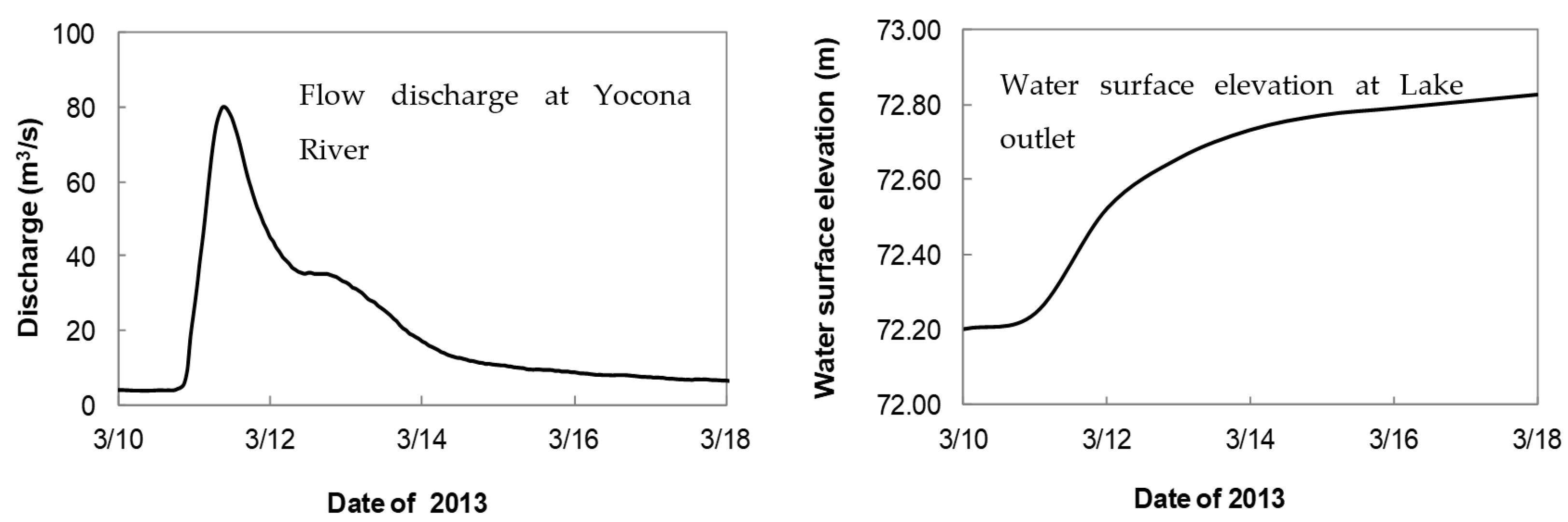
The upstream Yocona river flow discharge and water surface elevation at the lake outlet were obtained from USGS and US Army Corp of Engineers. Figure 2 shows the flow discharge and water surface elevation during a spring storm event that occurred in March 2013.

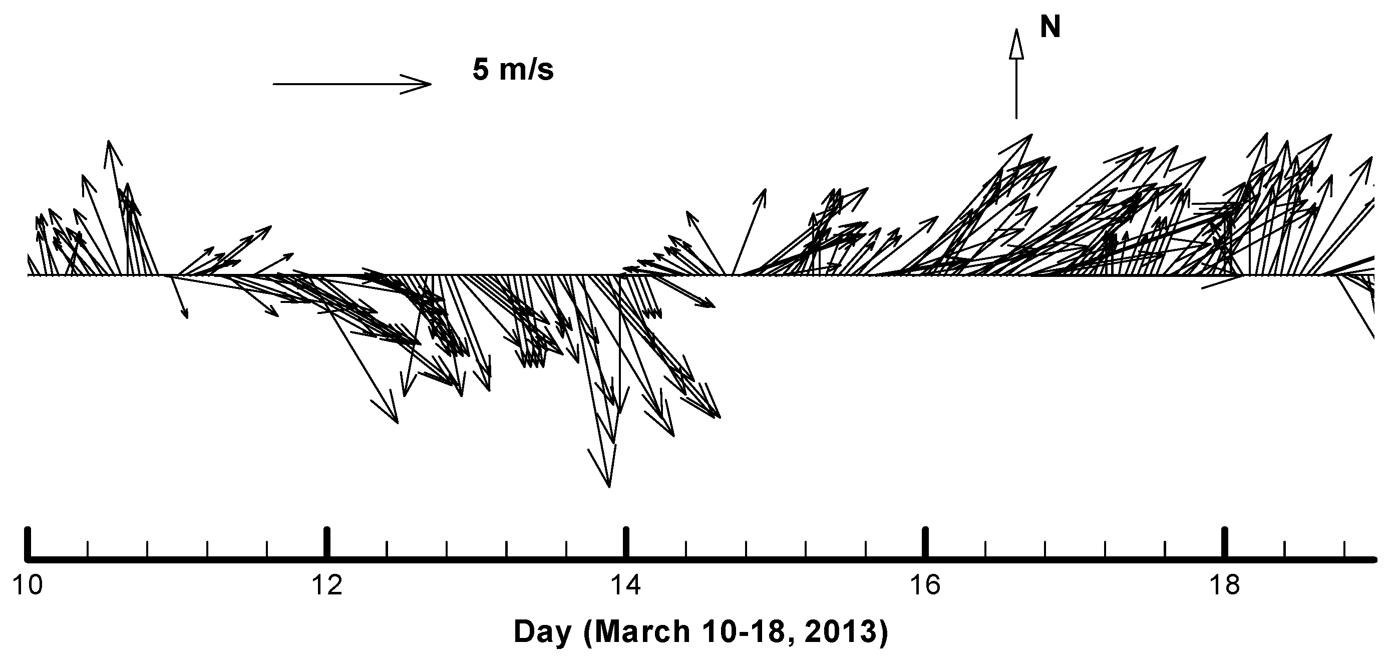
Wind is one of the most important driving forces for lake circulation. Figure 3 shows the wind speeds and directions near the lake during the study period (10 March 2013–18 March 2013) produced by the NOAA National Centers for Environmental Information.

4.3. Remote Sensing-Based Suspended Sediment Concentration Estimation

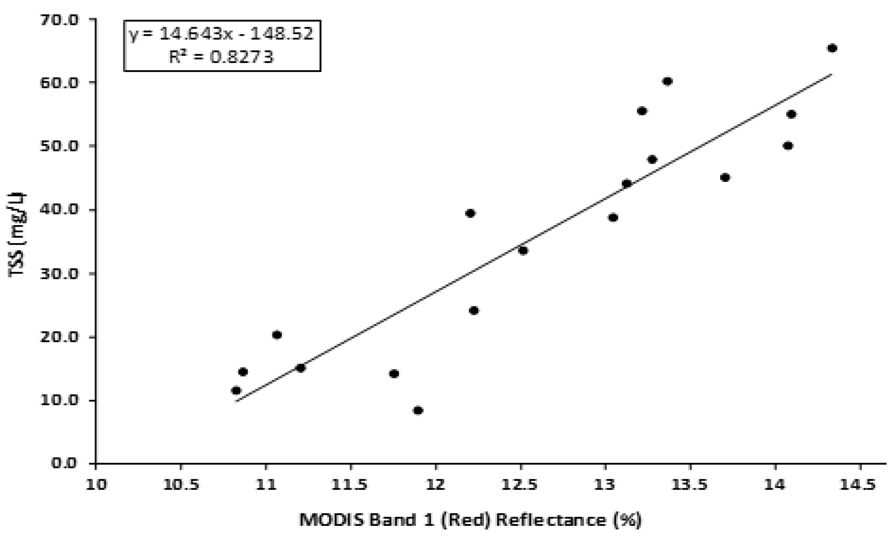
Several studies had success in estimating total suspended sediment (TSS) using simple linear regression techniques involving the MODIS visible and near-infrared (VNIR) bands and in situ measurements [6]. A similar approach was used in this study to estimate TSS in Enid Lake. The correlation coefficient of the regression equation was obtained using near-real time in situ measurements of TSS and the reflectance values of the red (R) and near infra-red (NIR) bands of the MODIS (Band 1 and Band 2) imagery acquired on 12 March 2013. The measured datasets include 18 in situ samples.

Figure 4 and Figure 5 show the correlation between the MODIS Reflectance of Red and NIR Bands (Band 1 and Band 2) and the TSS for 12 March 2013.

The obtained regression equation (Equation (16)) with a higher coefficient of determination (R²), as shown in Figure 4, was applied to the water pixels of the MODIS imagery to estimate the SSC in the lake at a 250 m spatial resolution. These 250 m spatial resolution estimations were then used to interpolate to a 1 m spatial resolution for the estimation of SSC in the lake water.

$$SS{C}_{MODIS}=14.643{\rho }_{Band1(Red)}-148.52$$

(16)

where SSC_MODIS is the MODIS-observed suspended sediment concentration and ρ_Band1(Red) is the surface reflectance recorded in the red spectral band (Band 1) of the MODIS sensor.

4.4. Numerical Model Simulation

Based on the initial bed elevation data obtained from the Enid Lake Fishing and Boating Map, the computational domain was discretized into a structured finite element mesh using the CCHE Mesh Generator. In the horizontal plane, two meshes with node numbers of 353 × 171 and 705 × 341 were employed to test the sensitivity of the mesh grid size on the numerical results. In the vertical direction, as this is a shallow lake, the domain was divided into eight layers based on the local water depth using a uniformly distributed function. For the case of wind-induced flow circulation in a big and shallow lake (mean water depth is less than 5 m), 8 to 10 vertical layers should be appropriate for model simulation [15]. The CCHE3D model was applied to simulate the wind-induced flow circulations using two meshes with 353 × 171 × 8 nodes and 705 × 341 × 8 nodes. The simulation results showed that the flow patterns obtained using two meshes were identical and that the maximum difference of the flow velocity was less than 1%. Therefore, the mesh with 353 × 171 × 8 nodes was used for the model simulation in this study.

4.4.1. Model Calibrations

In CCHE3D, several parameters, such as the parameter α in the Smagorinsky scheme (Equation (4)), drag coefficient C_d (Equations (7) and (8)) and bed roughness height need to be calibrated. A period from 17–25 November 2013, was selected for the model calibration run. In this period, wind was the main driving force for lake flow circulation. On 19 November, the USDA National Sedimentation Laboratory (NSL) measured flow velocities in the lake using an Acoustic Doppler Current Profiler (ADCP). The measured data was used for model comparison. After obtaining the measured wind data produced by NOAA, CCHE3D was used to simulate the wind-induced flow circulation in Enid Lake. The above-mentioned parameters were adjusted repeatedly to obtain a reasonable reproduction of the flow velocities measured by NSL. In this study, α = 0.1, C_d = 0.001 and bed roughness height = 0.02 m. The simulated flow velocities in the x and y directions at Station A (shown in Figure 1) were compared with the field-measured data (Figure 6). The flow velocities produced by the numerical model were generally in good agreement with field measurements.

The measured median diameter of the sediment particles was around 0.0025 to 0.003 mm, well within the cohesive sediment size. The settling velocities estimated using Equations (10) and (11) were in the order of 10⁻⁴ to 10⁻⁵ m/s. The critical shear stresses for deposition (${\tau }_{cd}$) and for erosion (${\tau }_{ce}$) in Equations (14) and (15) varied widely and needed to be calibrated. Since there was no sufficient measured sediment data in Enid Lake, the values of ${\tau }_{cd}$ and ${\tau }_{ce}$ were obtained based on our previous studies on a nearby lake (Deep Hollow Lake) with similar sediment size classes [16]. In this study, ${\tau }_{cd}$ = 0.01 N/m² and ${\tau }_{ce}$ = 0.02 N/m².

4.4.2. Model Applications

A simulation period from 10–18 March 2013 was selected for the model application to Enid Lake. In this period, the wind and upstream river discharge were the main driving forces for lake flow circulation. After setting up the inlet boundary conditions (flow and SS discharges) and outlet boundary conditions (water level), as well as the wind fields, the developed model could be applied to simulate the flow and cohesive sediment transport in the lake. In the model simulation, the parameters were the same as the calibrated values.

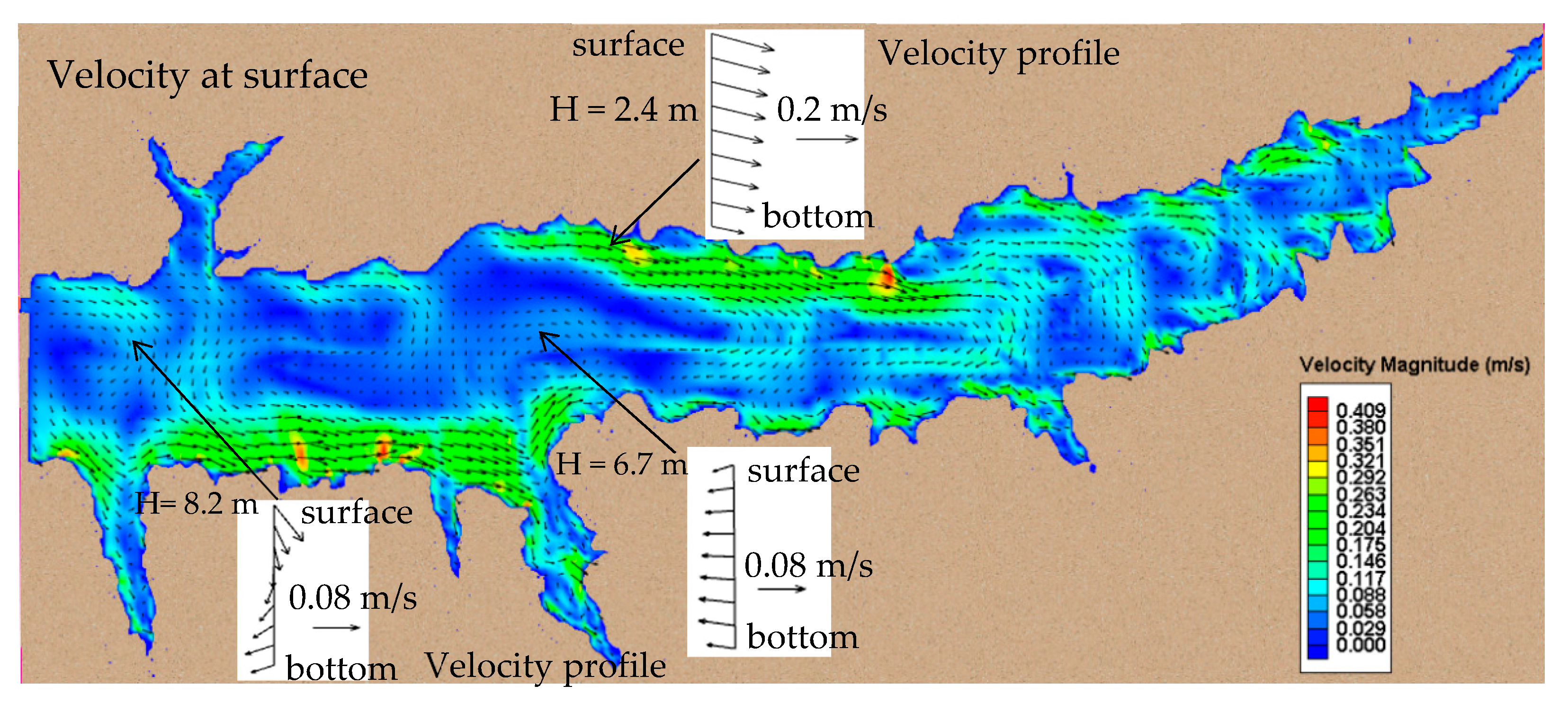
Figure 7 and Figure 8 shows the flow velocities at the water surface and near the bed (12 March 2013), which was induced by the upstream river discharge as well as the wind forces. The vertical velocity profiles in deeper and shallower areas were also plotted for comparison. In general, the velocities in shallower regions were stronger than those in deeper regions (Section 5 gives a detailed discussion).

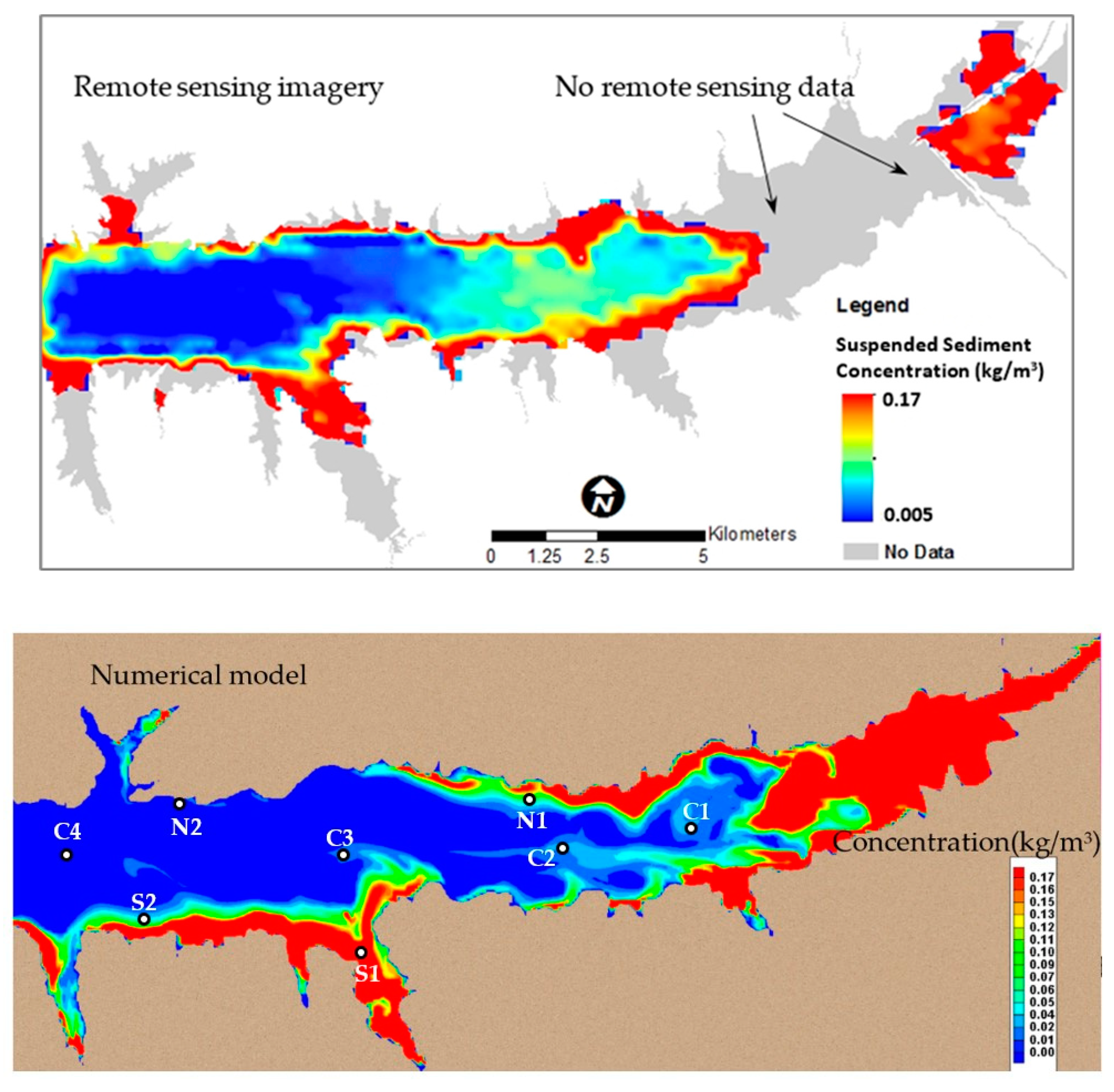
Figure 9 shows the comparison of concentrations of cohesive sediment at the surface of the lake obtained by numerical modeling and remote sensing technology (on 12 March 2013). The simulated results were generally in agreement with the data obtained with the remote sensing technology. Both the remote sensing data and numerical results showed the maximum SS concentration in the lake as being about 0.17 kg/m³. The SSC was higher near the river mouth and along shoreline areas, while it was much lower in the deeper water near the dam. Figure 9 shows that the numerical model underestimated the SSC along the northwest shoreline (near N2) and lake central area (near C2) compared to the remote sensing data. The possible reasons causing these differences are discussed in Section 5.

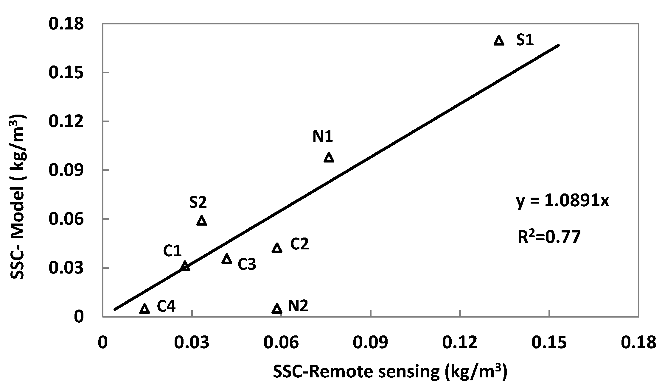
The SSC at several check points from the central area (C1, C2, C3, C4), north shoreline (N1, N2) and south shoreline (S1, S2) were extracted from the remote sensing data and model results for comparison. Figure 10 shows that the simulated SSC agreed with the remote sensing data, with a reasonable coefficient determination (R²) value of 0.77.

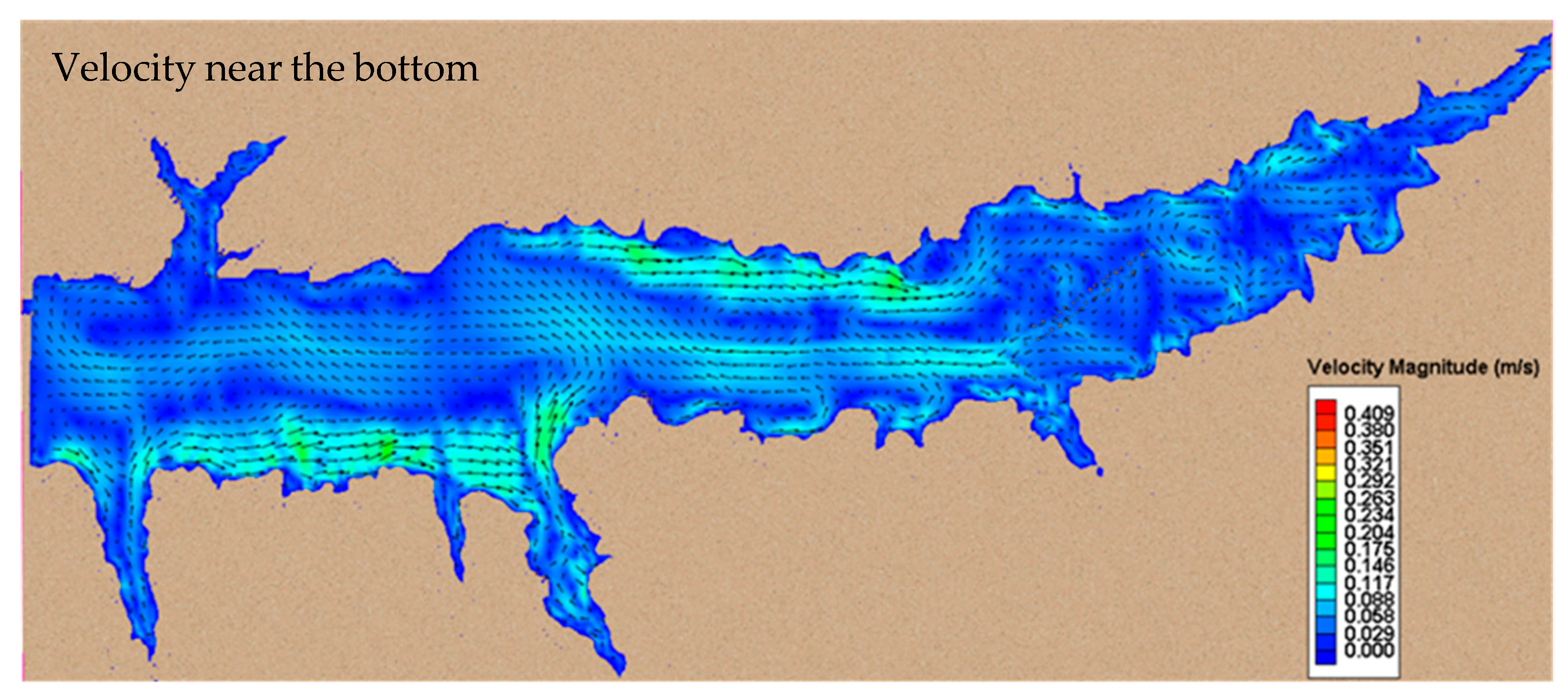
Figure 11 shows the simulated concentrations of cohesive sediment near the bottom of the lake. The sediment concentration in the lake is generally affected by the flow velocity, turbulent diffusion and settling velocity. Since the size of the cohesive sediment is very fine (0.0025~0.003 mm), the gradient of the vertical concentration of sediment is small. Figure 11 shows that the SSC in the central areas of the lake were slightly higher near the bottom than those at the water surface. In the shallow area, the SS was well mixed and the SSCs near the bottom and water surface were very close.

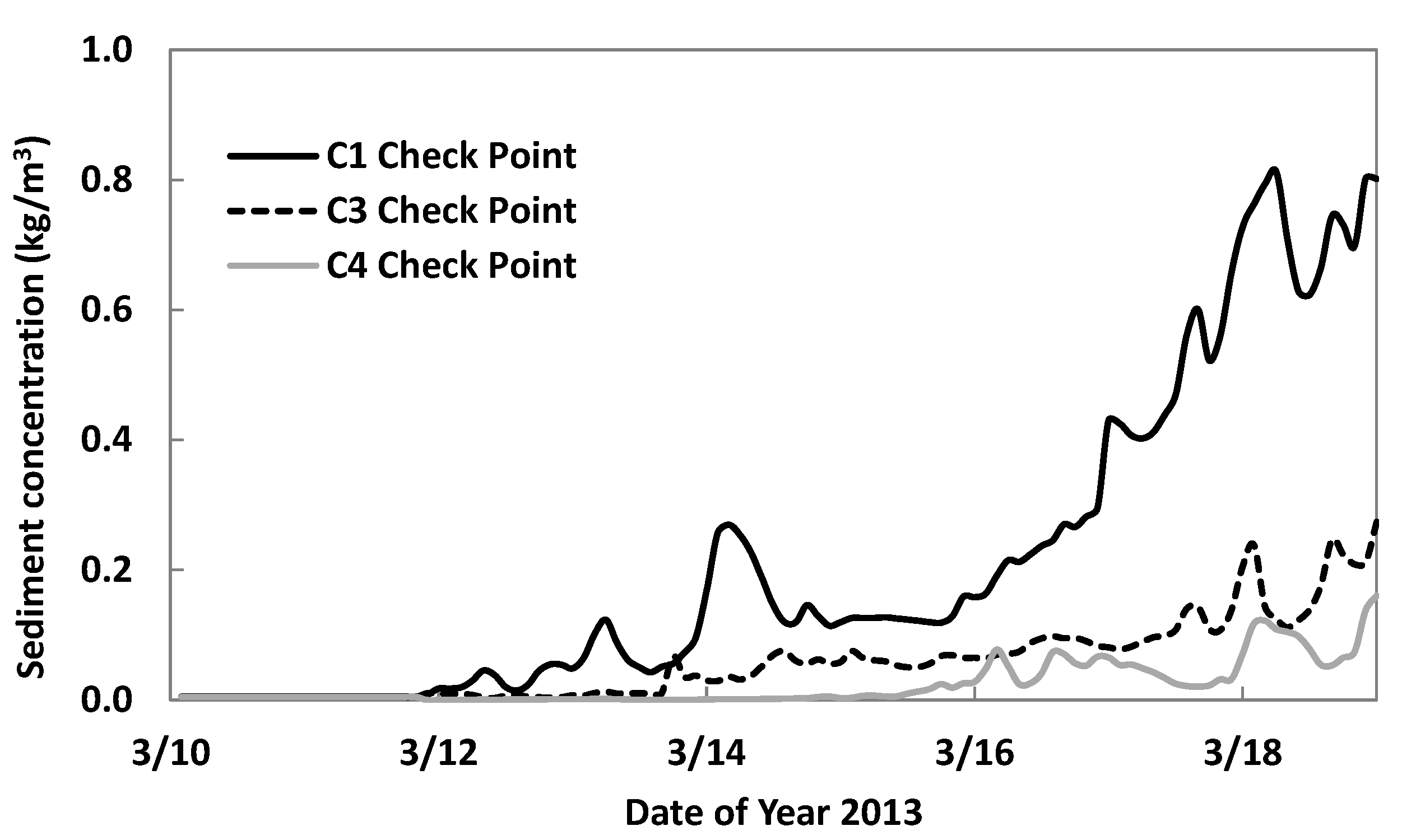
In general, the mean SSC in the lake was very low (~0.005 kg/m³). During the storm event, a large amount of sediment discharged into the lake from the upstream Yocona River. Figure 12 shows the time series of SSC at the water surface at check points C1 (upstream), C3 (mid-reach) and C4 (downstream; Figure 9). For the simulation, the sediment plume passed the check point C1 on 12 March. Around one and half days later, it reached the C3 point. On 15 March, the plume reached the area near the dam. In general, the SSC in the upstream of the lake (near C1) was much higher than that in the downstream.

5. Discussion

5.1. Three-Dimensional Flow Patterns in the Lake

The CCHE3D model was applied to simulate the flow hydrodynamics in Enid Lake during a spring storm event. Flow patterns in the lake are generally induced by wind force and upstream river flow discharge. Figure 7 and Figure 8 show flow patterns (12 March 2013) which indicate that the river discharges affect the flow fields near the river mouth (east parts) of the lake, and that the wind stress dominates the flow circulations of the entire lake. During this period, the major wind directions were coming from the northwest (Figure 3). In the shallow areas (near the north and south shorelines), flow patterns generally followed the wind directions, and the velocity magnitudes were also stronger than those in deeper regions. The velocity profile in shallow water (Figure 7) showed that the velocities at the water surface and near the bottom had the same directions, and that the bottom velocity was relatively smaller. While in the deeper regions, the flow patterns were very complex and the water velocities at the surface and bottom could turn towards different directions. The velocity profile near the dam showed that the flow circulations at the surface followed the wind direction, blowing from the northwest, while they turned to the inverse direction near the bottom (Figure 7). The velocity profile near the middle reach of the lake showed that the flow on the surface moved to the southwest, while it turned to the northwest at the bottom.

5.2. SS Concentration Distributions in the Lake

The sediment in Enid Lake primarily comes from the upstream Yocona River. During storm events, a large amount of SS discharges into the lake. The median diameter of sediment particles in the lake is very fine (around 0.0025 to 0.003 mm), and SSC in the lake is generally affected by the processes of advection, turbulence diffusion, sediment deposition and resuspension. Figure 9 and Figure 12 show that the SS plume moved westward and quickly occupied the upstream of the lake and gradually propagated to the mid-reach and downstream. Due to the process of deposition, the SSC in the mid-reach and downstream were much lower than that in the upstream. Figure 9 shows that the SSC near the north and south shorelines had reached certain levels before the SS plume arrived. This was due to the effects of wind-driven flow. Figure 7 shows that the wind-induced flow velocities in those shallow shoreline areas were relatively strong, and that the wind-induced bed shear stresses were greater than the critical shear stress for erosion, causing the SS resuspension (Equation (15)).

Figure 9 and Figure 11 show that the SSCs at the water surface and near the bottom had similar distributions, with a slightly higher concentration near the bottom. This result was also observed by others [27]: with the decrease of sediment size, the sediment is distributed more uniformly in the vertical direction due to the turbulence diffusion.

In this study, a linear regression equation (Equation (16)) obtained from the measured SSC and satellite image reflectance was applied to map the SSC in Enid Lake. The remote sensing technology provided a useful tool for validating the numerical model results for SS simulation. On the other hand, the missing data in the satellite image for SS estimation (such as the grey areas in Figure 9) could also be obtained using the numerical model. In addition, numerical modeling not only provides the surface SSC, but also the SS distributions in the water column.

A numerical model has been developed based on CCHE3D to simulate the process of cohesive sediment transport in Enid Lake. Compared with remote sensing imagery, the SSC at the northwest shoreline and central area of the lake were underestimated by the numerical model. This might be caused by the limitations of numerical modeling in simulating bed shear stress due to the wind, which significantly affects the SS resuspension (Equation (15)). The bed shear due to the wind is determined by both wind-induced currents and waves. In this model, the wind-induced current was simulated; however, the effect of wind-induced waves on the sediment resuspension was not taken into account, which may cause underestimation of SSC in shallow areas of the lake. In addition, the processes of bank erosion and landslides were not considered in this model simulation, which may also affect the model results. In general, the wind speeds and directions near the water surface of a large lake, such as Enid Lake, may vary spatially. The wind data provided by one station might not be sufficient for simulating the wind driving force for the entire lake.

6. Conclusions

A 3D numerical model has been developed to predict the dynamic flow fields and the temporal and spatial concentrations of cohesive sediment over an entire lake. Based on the upstream river flow discharge, sediment concentration, outlet water surface elevation and wind conditions, the flow fields—including velocity, water level, eddy viscosity, and the concentration of cohesive sediment in the lake—could be solved. In the model, the general processes of cohesive sediment transport, including flocculation, settling, deposition and erosion, were considered. The developed model was calibrated using the field-measured data, and then it was applied to simulate a spring storm event in Enid Lake. The simulated cohesive sediment concentration (median diameter 0.0025 to 0.003 mm) was generally in agreement with satellite imagery. Model results and satellite imagery show that the concentration of sediment was higher near the river mouth and shallow shoreline area than that in the deeper water areas near the dam.

Remote sensing technology has been successfully used to estimate and map the distributions of SS at the entire lake surface following a storm event. It also provides useful information for numerical model validation. The results from this study are directly applicable to other large lake systems in Mississippi and elsewhere.

Remote sensing and numerical modeling are both useful tools for the estimation and mapping of sediment concentrations in large lakes. This research demonstrates their advantages for sediment studies in large waterbodies by integrating the numerical model and remote sensing data; remote sensing can provide initial condition and validation data for numerical modeling; numerical modeling can simulate the spatial and temporal distributions of sediment concentration for the entire waterbody, which may provide useful information for estimating missing remote sensing data and mapping SS distributions under the water surface.

References

- Wu, W.; Wang, S.S.Y. Depth-Averaged 2-D Calculation of Tidal Flow, Salinity and Cohesive Sediment Transport in Estuaries. Int. J. Sed. Res. 2004, 19, 172–190. [Google Scholar]
- Liu, W.C. Modelling the Effects of Reservoir Construction on Tidal Hydrodynamics and Suspended Sediment Distribution in Danshuei River Estuary. Environ. Model. Softw. 2007, 22, 1588–1600. [Google Scholar] [CrossRef]
- Normant, C.L. Three-Dimensional Modeling of Cohesive Sediment Transport in the Loire Estuary. Hydrol. Process. 2000, 14, 2231–2243. [Google Scholar] [CrossRef]
- Klassen, I. Three-dimensional Numerical Modeling of Cohesive Sediment Flocculation Processes in Turbulent Flows. Ph.D. Thesis, Karlsruhe Institute of Technology, Karlsruhe, Germany, 2017. [Google Scholar]
- Gailani, J.; Ziegler, C.K.; Lick, W. Transport of Suspended Solids in the Lower Fox River. J. Great Lakes Res. 1991, 17, 479–494. [Google Scholar] [CrossRef]
- Wang, X.; Wang, Q.; Wu, Q. Estimating Suspended Sediment Concentration in Coastal Water of Minjiang River Using Remote Sensing Images. J. Remote Sens. 2003, 7, 54–57. [Google Scholar]
- Binding, C.E.; Bowers, D.G.; Mitchelson-Jacob, E.G. Estimating Suspended Sediment Concentrations from Ocean Color Measurements in Moderately Turbid Waters; The Impact of Variable Particle Scattering Properties. Remote Sens. Environ. 2005, 94, 373–383. [Google Scholar] [CrossRef]
- Pavelsky, T.M.; Smith, L.C. Remote Sensing of Suspended Sediment Concentration, Flow Velocity, and Lake Recharge in the Peace-Athabasca Delta, Canada. Water Resour. Res. 2009, 45, W11417. [Google Scholar] [CrossRef]
- Hossain, A.; Jia, Y.; Chao, X. Development of Remote Sensing Based Index for Estimating/Mapping Suspended Sediment Concentration in River and Lake Environments. In Proceedings of the 8th International Symposium on ECOHYDRAULICS (ISE 2010), COEX, Seoul, Korea, 12–16 September 2010; Volume 435, pp. 578–585. [Google Scholar]
- Montanhera, O.C.; Novoa, E.M.L.M.; Barbosaa, C.C.F.; Rennóa, C.D.; Silva, T.S.F. Empirical Models for Estimating the Suspended Sediment Concentration in Amazonian White Water Rivers Using Landsat 5/TM. Int. J. Appl. Earth Obs. Geoinf. 2014, 29, 67–77. [Google Scholar] [CrossRef]
- Jia, Y.; Scott, S.; Xu, Y.; Huang, S.; Wang, S.S.Y. Three-Dimensional Numerical Simulation and Analysis of Flows around a Submerged Weir in a Channel Bendway. J. Hydraul. Eng. 2005, 131, 682–693. [Google Scholar] [CrossRef]
- Jia, Y.; Scott, S.; Xu, Y.; Wang, S.S.Y. Numerical Study of Flow Affected by Bendway Weirs in Victoria Bendway, the Mississippi River. J. Hydraul. Eng. 2009, 135, 902–916. [Google Scholar] [CrossRef]
- Wang, S.S.Y.; Roche, P.J.; Schmalz, R.A.; Jia, Y.; Smith, P.E. Verification and Validation of 3D Free-Surface Flow Models; American Society of Civil Engineering: Reston, VA, USA, 2008. [Google Scholar]
- Koutitas, C.; O’Connor, B. Modeling Three-Dimensional Wind-Induced Flows. J. Hydraul. Div. 1980, 106, 1843–1865. [Google Scholar] [CrossRef]
- Chao, X.; Hossain, A.K.M.A.; Jia, Y. Three Dimensional Numerical Modeling of Flow and Pollutant Transport in a Flooding Area of 2008 US Midwest Flood. Am. J. Clim. Chang. 2013, 2, 116–127. [Google Scholar] [CrossRef] [Green Version]
- Chao, X.; Jia, Y.; Shields, F.D., Jr.; Wang, S.S.Y.; Cooper, C.M. Three-Dimensional Numerical Modeling of Water Quality and Sediment-Associated Processes with Application to a Mississippi Delta Lake. J. Environ. Manag. 2010, 91, 1456–1466. [Google Scholar] [CrossRef] [PubMed]
- Burban, P.Y.; Xu, Y.J.; Mcneil, J.; Lick, W. Settling Speeds of Flocs in Fresh Water and Seawater. J. Geophys. Res. 1990, 95, 18213–18220. [Google Scholar] [CrossRef]
- Lick, W.; Lick, J. Aggregation and Disaggregation of Fine-Grained Lake Sediments. J. Great Lakes Res. 1988, 14, 514–523. [Google Scholar] [CrossRef]
- Krone, R.B. Flume Studies on the Transport of Sediment in Estuarine Shoaling Processes, Hydraulic Engineering Laboratory; Technical Report for University of California: Berkeley, CA, USA, 1962. [Google Scholar]
- Mehta, A.J.; Partheniades, E. An Investigation of the Depositional Properties of Flocculated Fine Sediment. J. Hydraul. Res. 1975, 13, 361–381. [Google Scholar] [CrossRef]
- Partheniades, E. Erosion and Deposition of Cohesive Soils. J. Hydraul. Div. 1965, 91, 105–139. [Google Scholar] [CrossRef]
- Van Rijn, L.C. Handbook Sediment Transport by Currents and Waves; Delft Hydraulics: Delft, The Netherlands, 1989. [Google Scholar]
- Bennet, S.J.; Rhoton, F.E. Linking Upstream Channel Instability to Downstream Degradation: Grenada Lake and the Skuna and Yalobusha River Basin, Mississippi. Ecohydrology 2009, 2, 235–247. [Google Scholar] [CrossRef]
- Wolff, S.; Brown, G.; Chen, J.; Meals, K.; Thornton, C.; Brewer, S.; Cizdziel, J.; Willett, K. Mercury Concentrations in Fish from Three Major Lakes in North Mississippi: Spatial and Temporal Differences and Human Health Risk Assessment. J. Toxicol. Environ. Health Part A 2016, 79, 894–904. [Google Scholar] [CrossRef] [PubMed]
- Mississippi Department of Environmental Quality (MDEQ). Yocona River and Enid Reservoir Phase One Total Maximum Daily Load For Mercury; Mississippi Department of Environmental Quality (MDEQ): Jackson, MS, USA, 2002. [Google Scholar]
- Huggett, D.B.; Steevensa, J.A.; Allgoodb, J.C.; Lutkenc, C.B.; Gracec, C.A.; Benson, W.H. Mercury in Sediment and Fish from North Mississippi Lakes. Chemosphere 2001, 42, 923–929. [Google Scholar] [CrossRef]
- Li, Y.; Xie, L.; Su, T.C. Vertical Distribution of Suspended Sediments above Dense Plants in Water Flow. Water 2020, 12, 12. [Google Scholar] [CrossRef] [Green Version]