
Suitability of Screened Monitoring Wells for Temperature Measurements Regarding Large-Scale Geothermal Collector Systems


GeoZentrum Nordbayern, Department Geographie und Geowissenschaften, Friedrich-Alexander-Universität Erlangen-Nürnberg, Schlossgarten 5, 91054 Erlangen, Germany
*
Author to whom correspondence should be addressed.
Geosciences 2022, 12(4), 162; https://0-doi-org.brum.beds.ac.uk/10.3390/geosciences12040162
Submission received: 7 March 2022
/
Revised: 25 March 2022
/
Accepted: 29 March 2022
/
Published: 4 April 2022
(This article belongs to the Section Hydrogeology)
Abstract
:Groundwater temperature (GWT) is usually measured using screened monitoring wells (MWs). The aim of this study was to investigate whether MWs are suitable for monitoring the effects of large-scale geothermal collector systems (LSCs) on GWT, focusing on possible vertical flows within the MWs due to both natural and forced convection. Comparative temperature depth profiles were therefore recorded over a period of nine months in both shallow MWs and in small-diameter, non-screened temperature monitoring stations (TMSs), each of which was installed in a single borehole. Particularly high temperature deviations were measured in MWs in the upper part of the water column where the GWT reached up to 1.8 K warmer than in the surrounding subsurface. These deviations correlate unambiguously with the prevailing positive thermal gradients and are caused by thermal convection. Where forced convection occurred, the GWT was measured to be up to 0.8 K colder. Potential temperature deviations must be considered when monitoring very shallow GWT as thermal gradients can be particularly high in these zones. For monitoring concepts of LSCs, a combination of MW and TMS is proposed for GWT measurements decoupled by the effects of convection and in order to enable further investigations such as pumping tests.
1. Introduction
1.1. Importance of Monitoring Groundwater Temperature
Conduction is the dominant heat transport mechanism in unsaturated soils [1]. The thermal conductivity of an unsaturated soil depends on a number of soil parameters [2,3,4,5,6] and on temperature [7]. In addition to conduction, convection is another important means of heat transport in aquifers [8]. The groundwater flow rate can therefore influence the effective thermal conductivity of an aquifer [9]. The temperature of the shallow subsurface is mostly determined by the climatic conditions at the surface. Shallow groundwater temperature (GWT) is affected by vertical heat transfer in the unsaturated zone down to depths of 10 to 15 m [10]. Rising temperatures due to climate change [11,12,13] or to heated underground structures and artificial surface sealing in urban areas [14,15,16,17] can therefore have an impact on GWT.
A further anthropogenic factor that can influence shallow GWT is the use of geothermal energy systems, which continues to increase since in addition to climate friendly power generation, the provision of energy for heating is also an important factor [18]. The thermal impact of open-loop systems and borehole heat exchangers on GWT is well studied [19,20,21]. For very shallow systems, such as horizontal ground heat exchangers, studies have focussed predominately on soil temperatures in the unsaturated zone [22,23,24,25,26,27]. However, for large-scale geothermal collector systems (LSC) [28], their possible impact on GWT, especially in areas with a shallow groundwater level, needs to be considered to ensure sustainability and to prevent interference between neighbouring geothermal systems. It is also important to note that altering the thermal conditions of the subsurface can bear ecological and geochemical impacts [29,30,31,32]. Negative changes in groundwater quality due to thermal alterations must be averted [33]. Therefore, predicting the thermal effects on GWT represents a potentially important element in the statutory approval process for geothermal systems. Hähnlein et al. [34] recommend that the sustainable thermal use of shallow geothermal energy should be based on technical assessment, environmental assessment and monitoring, whereby the environmental assessment would include temperature thresholds and groundwater quality criteria. In general, this means groundwater monitoring wells (MWs) are required for monitoring GWT and groundwater sampling.
1.2. Vertical Flows in MWs due to Convection
Ordinary screened MWs with diameters ≥50 mm are often used to monitor GWT. However, the temperatures measured in MWs can be influenced by vertical flows within the well [35]. These flows can be caused by forced convection resulting from hydraulic gradients, since the MWs are hydraulically connected by the well screen to different permeable layers in the subsurface. Therefore, in addition to temperature measurements, groundwater sampling and groundwater level measurements can also be influenced by forced convection [36,37].
Another possible cause of vertical flow in MWs or in boreholes is natural (or free) convection [35,38,39,40,41]. Unlike forced convection, natural convection can affect the water column in all directions [38]. Natural convection occurs as a result of density differences, when the ratio of the forces driving fluid movement to those retarding fluid flow exceed a certain critical value [42]. This ratio of driving to retarding forces is described by the dimensionless Rayleigh number Rat. The critical density gradients can be caused by temperature differences due to a downward positive thermal gradient. The critical thermal Rayleigh number–the threshold above which natural thermal convections starts–can be calculated for water columns in boreholes or MWs by considering the thermal conductivity of the fluid and the surrounding material [43]. In addition to thermal causes, natural convection can also be caused by density differences due to gradients in salinity or dissolved solids. Solutal convection and the combination of solutal and thermal convection is described in detail by Börner and Berthold [35].
According to Rayleigh [42] and Gershuni and Zhukhovitskii [43], and as summarised by Börner and Berthold [35], is calculated as follows:
where:
- = thermal Rayleigh number
- = gravitational acceleration [m/s2]
- = thermal expansion coefficient [1/K]
- = radius of water column [m]
- = kinematic viscosity [m2/s]
- = thermal diffusivity [m2/s]
- = thermal gradient [K/m]
A fluid’s therefore depends on the diameter of the water column and the temperature of the fluid. According to Börner and Berthold [35] a critical thermal Rayleigh number of 148 can be applied for typical subsurface zones based on a thermal conductivity value for water of 0.6 W/mK and for the surrounding rock of 2.1 W/mK. Table 1 shows for different monitoring well diameters and a range of water temperatures, the critical thermal gradient at which the Rayleigh number exceeds the critical value of 148 and thermal convection begins.
As can be seen in Table 1, the critical thermal gradient decreases with increasing diameter of the water column and increasing fluid temperature. When conducting GWT measurements, it is therefore advisable to select the smallest possible diameter for the MWs so that the measurements are not distorted by natural convection in the water column. However, in addition to temperature measurements, additional investigations, such as pumping tests or groundwater sampling, are often required for which sufficiently large diameter MWs are needed. If, as is often the case, large diameter wells are used for temperature measurements, possible temperature deviations due to convection need to be estimated and accounted for.
1.3. Aims of This Study
According to current knowledge, the thermal impact of LSCs on GWT has not yet been investigated. Such a study will require temperature monitoring concepts to be created in advance. This paper discusses whether ordinary MWs are suitable for the thermal monitoring of such systems and which factors need to be accounted for. For this reason, the aim of the study was to determine how the well screen and the diameter of the well casing–two parameters that can influence convection–affect GWT measurements in the shallow subsurface.
Forced convection has been investigated using chemical samples and geophysical measurements [36]. Natural convection has thus far been investigated in the laboratory, through modelling, particle velocity image measurements or geophysical borehole measurements [38,41,44,45]. Berthold and Börner [38] proposed two algorithms based on high-resolution geophysical borehole measurements that would facilitate detection of the causes and effects of natural convection. These studies focused mainly on short-term temperature deviations or temperature oscillations at a certain depth, rarer on actual seasonal temperature deviations and the locations where they occur.
The present study aims to investigate the influence of convection by making comparative GWT measurements. To this end, GWT measurements were conducted in six MWs over a period of nine months. In addition, non-screened small-diameter temperature measurements stations (TMSs) that were filled with water were installed in the same boreholes. Due to the lack of screens and the small diameter, convection-driven vertical flows in the TMSs were either non-existent or significantly weakened (Table 1). The depth profile measurements were recorded with an accuracy and resolution typical for practical hydrogeological applications, so that the results could be transferred to other locations and other projects. The objective is to detect temperature deviations in the MWs to determine the influence of convection and of the thermal gradient in the subsurface, including seasonal variations, and to develop a proposal for temperature monitoring concepts for LSCs.
2. Materials and Methods
2.1. Study Site and Hydrogeological Conditions
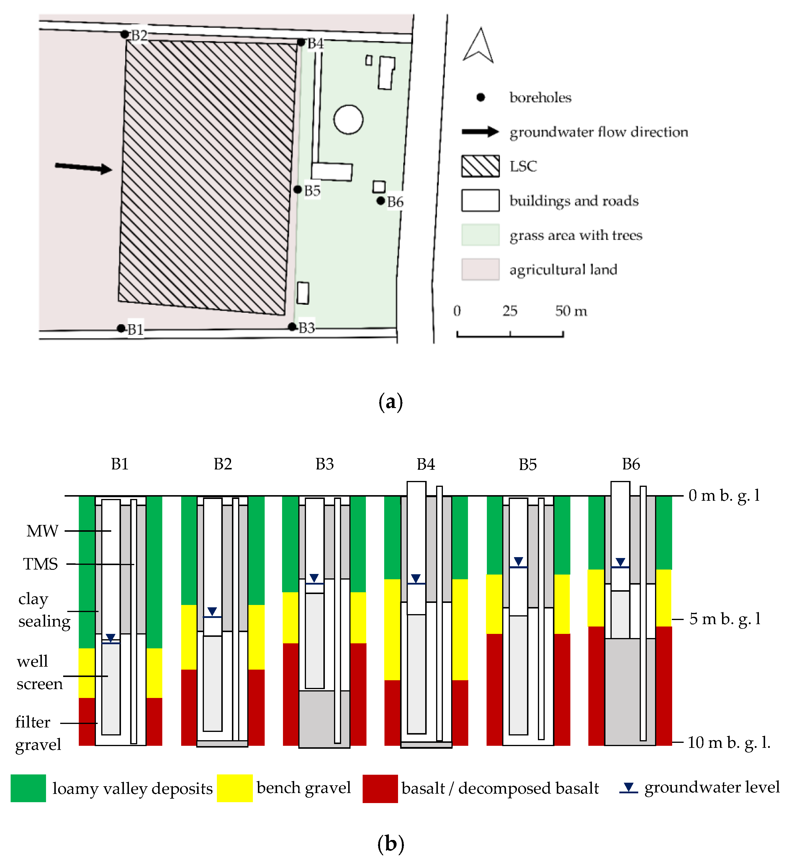
The test site was located at Bad Nauheim, a city in Hesse in the southwest of Germany. A two-layer LSC, which was described in detail by Zeh et al. [28] and covering a total area of 22,000 m2, was installed under agricultural land (Figure 1a). This system will provide heating and cooling energy for a new residential settlement via a low-temperature district heating network. Scientific evaluation and support are provided through the research project ‘KNW-Opt’ (Grant No. 03EN3020C). The groundwater monitoring system at the LSC site comprised six boreholes with a diameter of 220 mm that were located over a 14,000 m2 array. The maximum distance between neighbouring boreholes was 145 m and they were sunk to a depth of 10.5 m below ground level (m b. g. l.).
The LSC was not yet in operation during the measurement period. However, several test operations and leak tests were carried out, so that a certain thermal influence on the subsurface could be assumed. Therefore, the thermal conditions were considered disturbed and may deviate from natural conditions.
Bad Nauheim is located at the eastern edge of the Taunus mountain range. The shallow groundwater flows towards the river Usa, which is about 600 m away. Quaternary loamy valley deposits and bench gravels from the river Usa were found in the shallow subsurface at the test site [46]. These river deposits are overlain by topsoil and agricultural soil. The geological units encountered at each borehole are shown in Figure 1b and Table 2.
Several grain size analyses were performed, and the loamy valley deposits can be described as clayey silt with estimated permeabilities in the range k = 10−6 to 10−9 m/s [47]. This unit can therefore be characterised as an aquitard or semi-confining layer. The boundary to the bench gravel below occurs at varying depths and is not sharply delineated.
The quaternary bench gravel has a thickness of between 2.1 m and 4.3 m and is the local shallow aquifer. This gravel layer contains stones with an edge length of up to 0.15 m and interjacent finer layers of clayey silt. The permeability of the gravelly parts was estimated to be k ≈ 10−3 m/s [47]. At high groundwater levels, the groundwater is regarded as semi-confined due to the overlying loam. During the measuring period, the groundwater level had an amplitude of 1.1–1.2 m.
A very heterogeneous layer of tertiary basalt lies below the bench gravel. In the upper sections of the basalt layer, the basalt is mostly decomposed to clayey silt with clay sections. In B4, the basalt has decomposed to form a clay known as ‘Rotlehm’ [48]. Deeper down, the basalt has more solid rock characteristics and can be permeable (Table 2).
In each borehole, a MW with a diameter of 80 mm was installed. The well casing, borehole fillings and screen length are shown in Figure 1 and Table 2. The TMSs were fitted with non-screened PVC pipe with an inner diameter of 32 mm. By filling the TMS with water, the temperature in the saturated zone and above the groundwater level—in the unsaturated zone—can be measured. Due to leakage issues at the bottom of the TMSs and following adjustment of the water table to the groundwater level, PE pipes with a wall thickness of 3 mm and a diameter of 25 mm were additionally installed after the first measurement in February 2021. The water remained in the TMSs, thus at all measurements a thermal equilibrium was granted.
2.2. GWT and Electrical Conductivity Measurements
The temperature measurements were conducted once a month from February to October 2021. The temperature was recorded every 0.5 m starting from the groundwater table in the MWs or from the water table in the TMSs to the bottom of the well casing. The temperature was measured using a Solinst TLC-meter with a stated accuracy of ±0.1 K. The electrical conductivity (EC) of the groundwater was also recorded every 0.5 m with an accuracy of 2% of the reading value. The measurements were conducted on the following dates [DD-MM] in 2021: 03–02, 24–03, 22–04, 26–05, 23–06, 08–07, 19–08, 28–09 and 14–10.
To compare the temperatures measured in the MWs and in the TMSs in each borehole, the temperature difference at each measurement depth in the MWs was calculated as follows:
where:
- ΔTi = calculated temperature difference at the depth i [K]
- T(MW)i = measured temperature in MW at the depth i [°C]
- T(TMS)i = linearly interpolated temperature in TMS at the depth i [°C]
- i = depth [m b. g. l.]
- z = depth [m b. gw. l.]
Given the measurement accuracy of the TLC-meter, temperature differences were deemed significant when ΔT > 0.2 K.
3. Results
3.1. Temperatures and Differences between MWs and TMSs
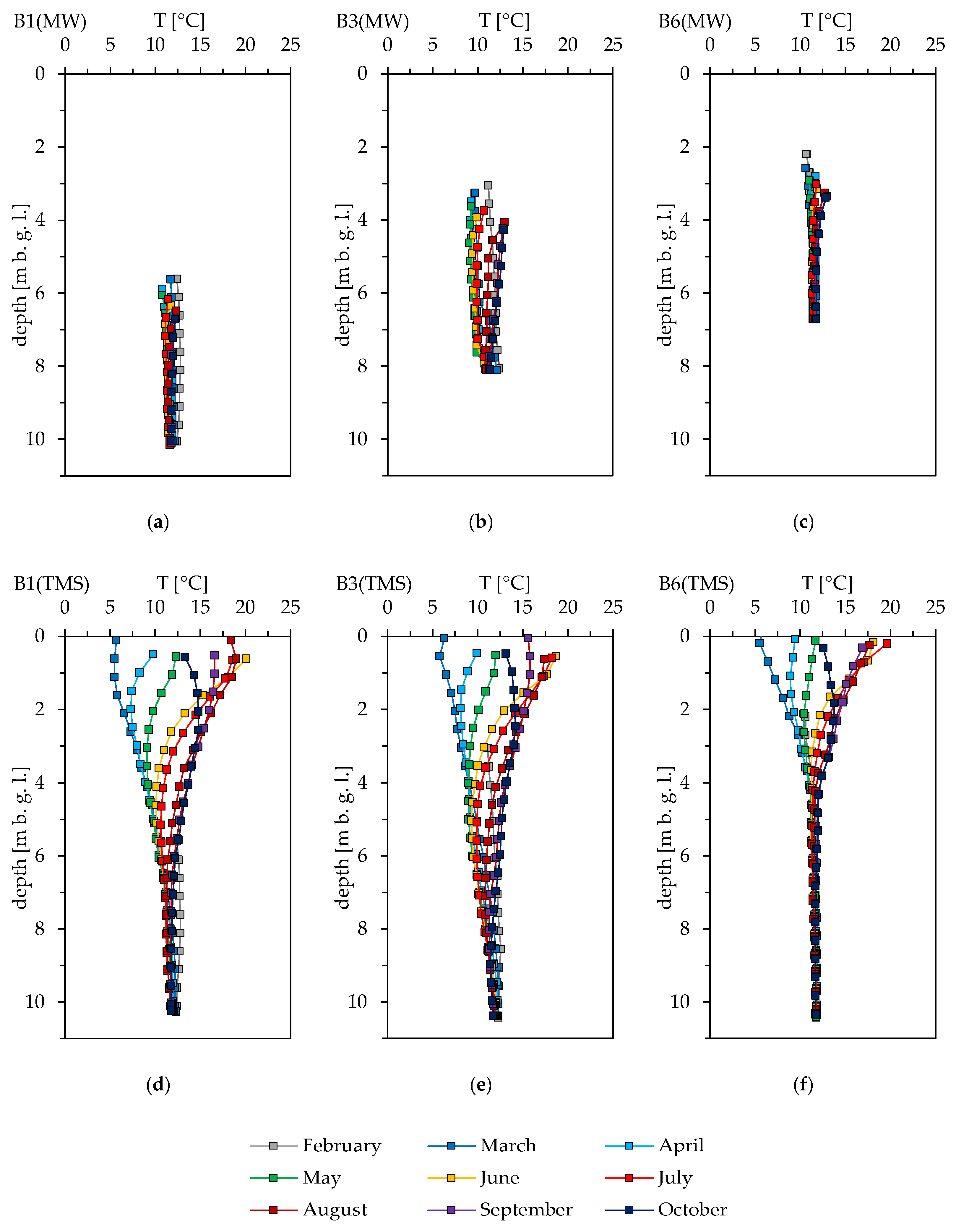
Figure 2 presents examples of temperature depth profiles measured in the MWs and TMSs for selected boreholes.
Temperature shifts were observed in each borehole over the nine-month measurement period. These shifts became more prominent with decreasing distance to ground level. As is apparent in Figure 2, the temperature shifts varied between boreholes. The temperature depth profiles recorded in the TMSs show the most significant temperature fluctuations in the first 4 m below ground level. While these fluctuations could still be observed at greater depths in other boreholes, in B6 the GWT measured in the TMS was approximately constant at depths of more than 4 m.
At the bottom of the MWs in boreholes B1, B2, B4 and B5 (i.e., at a depth of approximately 10 m b. g. l.), the GWT were between 10.8 °C and 12.4 °C with amplitudes of 0.8–1.1 K over the measuring period. Likewise, in the TMSs at depths of 10.0–10.4 m below ground level, temperatures of between 11.0 °C and 12.3 °C with amplitudes of 0.5–0.9 K were measured. It was only in the TMS in borehole B6, where a constant temperature of about 11.8 °C could be observed at this depth.
In contrast to the other MWs, in B3 significant jumps in the GWT were observed in the depth range 7.3–7.6 m below ground level, which is at least 0.5 m above the bottom of the well. These temperature jumps were measured from March to July. At these depths, the GWT rose by up to 1.2 K per 0.5 m. In March, the temperature in the depth range 6.3–6.8 m below ground level increased additionally at a rate of 1.1 K per 0.5 m. However, no equivalent rapid change of temperature was observed at those depths in the TMS.
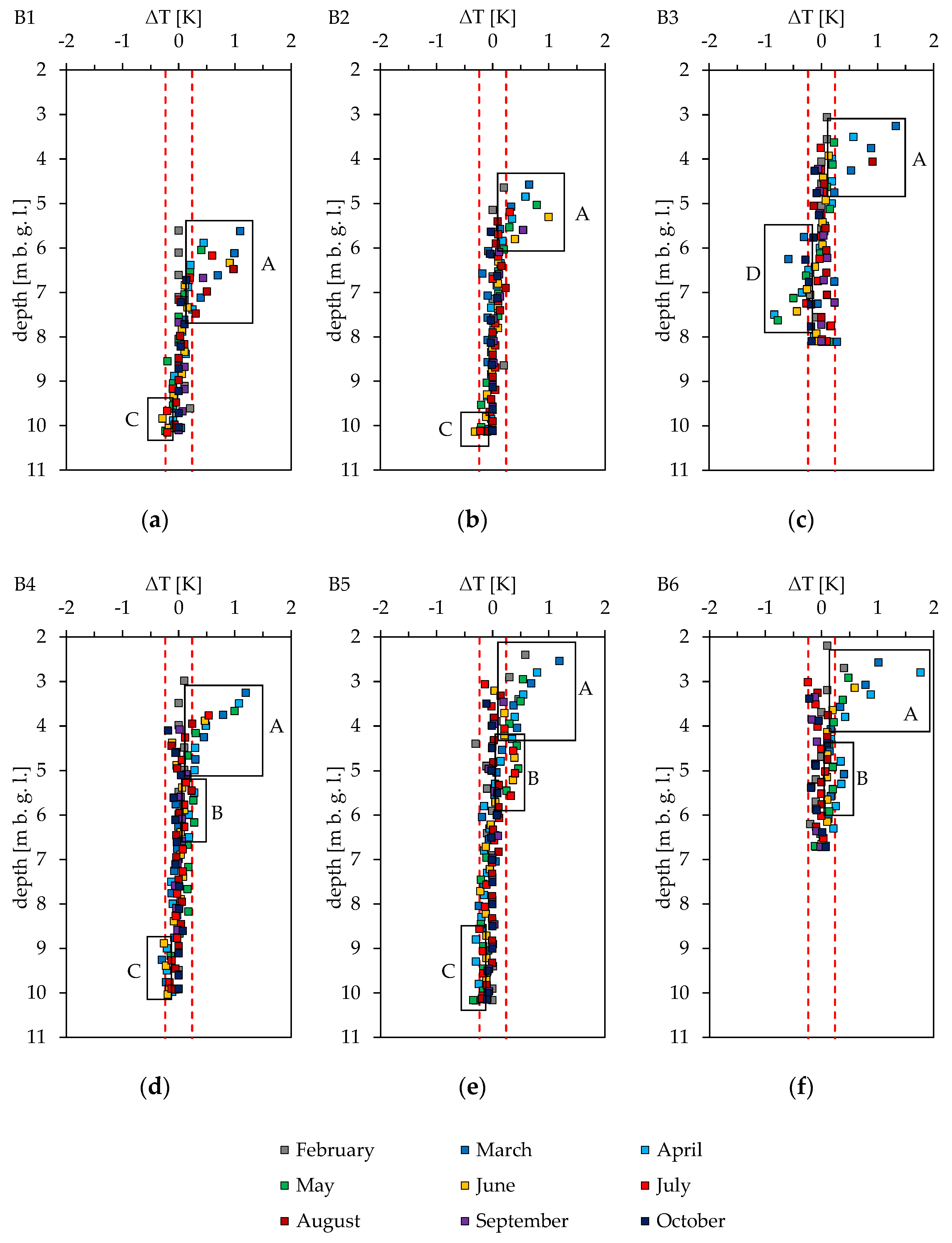
The ΔT values calculated using Equation (2) are shown for each borehole in Figure 3.
There are four distinct areas along the water column where significant values for ΔT occurred. These areas are marked in Figure 3. Area A was observed temporarily in each borehole and was located between the groundwater table and a depth of z = 1.5 below groundwater level depending on the borehole. The largest temperature differences with values up to 1.8 K were observed at the groundwater table. At z = 0.5 m, the maximum value of ΔT was 1.0 K while at z = 1.5 m, the maximum value was 0.4 K. The temperature difference between the MW and the TMS decreased with increasing depth. In this area (A), only positive values for ΔT were observed, i.e., higher temperatures were measured in the MWs than in the TMSs. Significant temperature differences in area A occurred predominately in the period March to May.
Area B was mainly observed in borehole B5 and less significantly in B4 and B6. In this area, which was not far below or overlaps with area A, positive values of ΔT of up to 0.5 K in B5 from May to July, 0.3 K in B4 in April and May and 0.4 K in B6 in March and April were observed.
Area C was identified in boreholes B1, B2, B4 and B5 close to the bottom of the MW. In this area, negative values of ΔT of −0.3 K were observed temporarily.
Area D only occurred in B3. This area is located in the depth range 5.8–7.6 m below ground level. From March to July and in October significant negative values of ΔT of up to 0.8 K were observed. Thus, in Area D, the MW produced temporary but significantly colder values of the GWT than those recorded in the TMS.
3.2. Electrical Conductivities in MWs
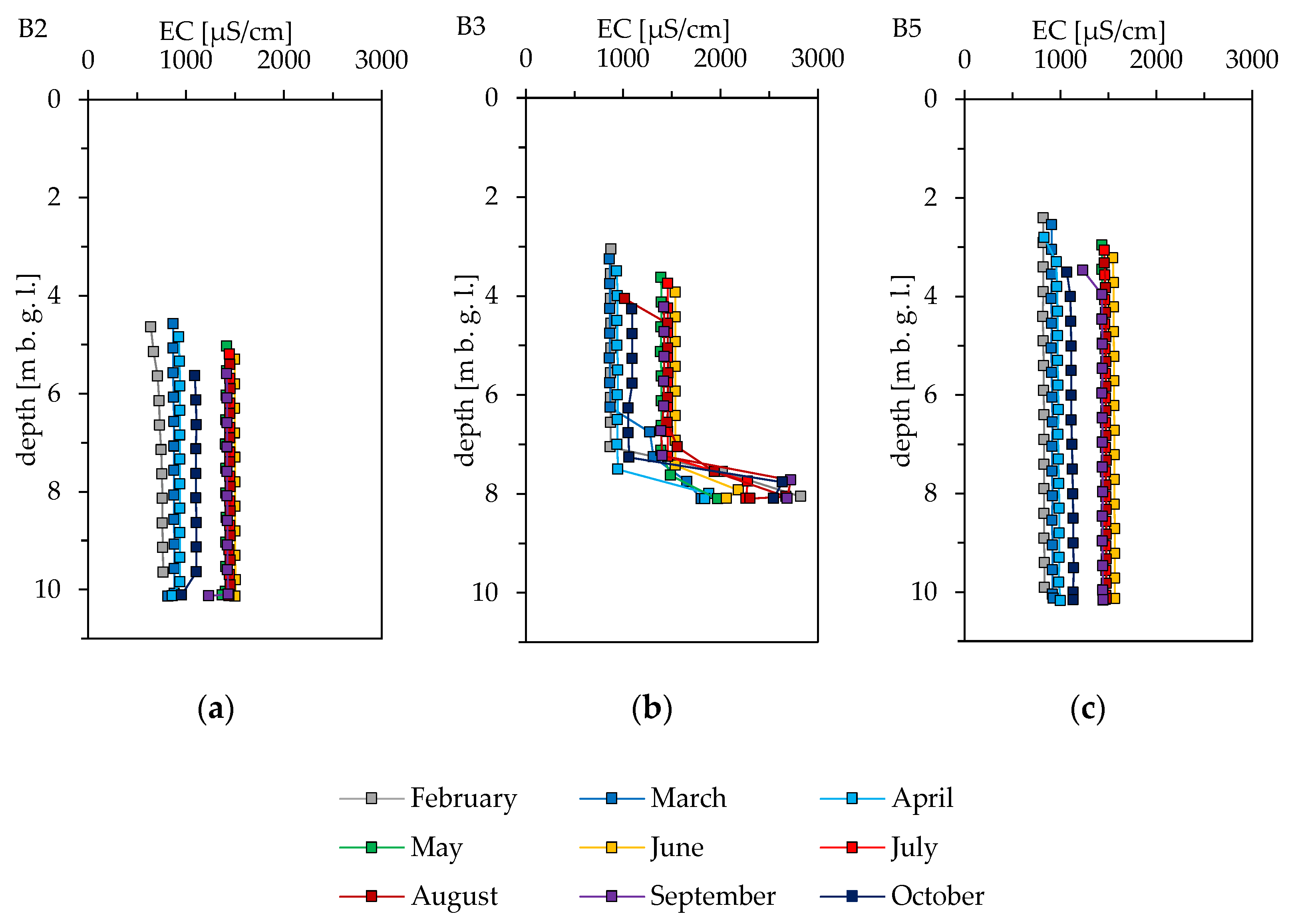
Examples of the electrical conductivity (EC) values measured in MWs are shown in Figure 4. In all boreholes, excluding B3, the EC depth profiles exhibit either constant but time-fluctuating EC values of between 700 μS/cm and 1600 μS/cm or a very slightly downward positive gradient. At the bottom of the MWs, lower EC values were often measured due to the small layer of mud present at these depths. Lower values were also measured at the groundwater table in some cases, which can be explained by the measurement uncertainty of the TLC-meter at the groundwater surface.
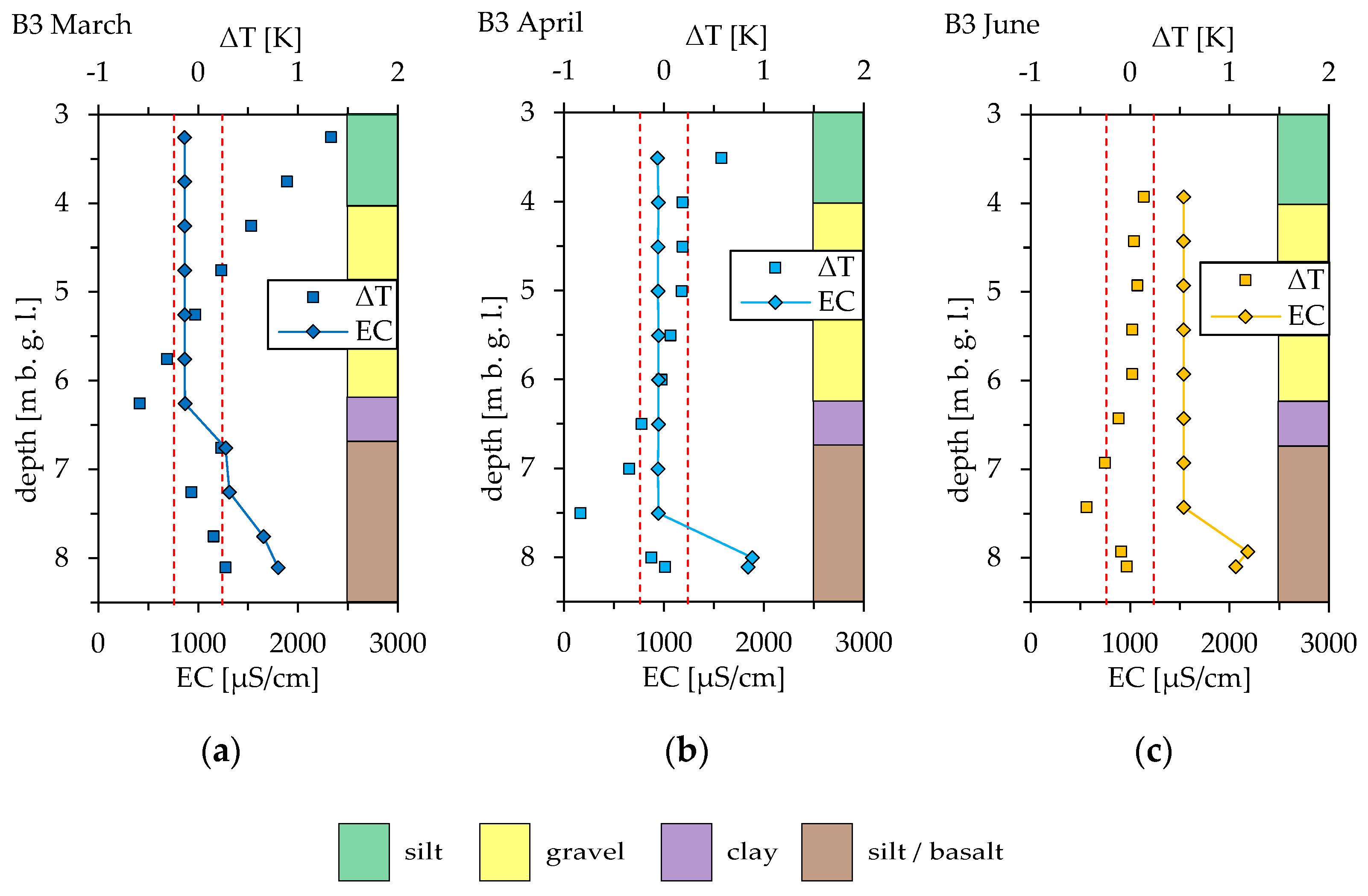
In the upper water column, the groundwater in B3 had similar EC values. However, regardless of when the measurements were performed, the values increased rapidly in the depth range 7.2–7.6 m and remained at a high level down to the bottom of the MW. The EC values increased by up to 1150 μS/cm per 0.5 m at this depth, reaching a maximum value of around 2800 μS/cm. In March and in August, smaller increases in the EC values were observed additionally in the depth range 6.3–6.6 m below ground level.
These rapid changes in the EC occurred at the same depths as the temperature jumps described in Section 3.1. As Figure 5 shows, negative values of ΔT (Area D) occurred above the jumps in the EC and GWT values during the period March to July.
From April to July, Area D was located in the partially permeable silt layer of the tertiary basalt where basalt rocks are also present. This is the area in which the significant shifts in EC and GWT values were observed. However, in March, Area D was located in the gravel layer with higher values of GWT and EC already measured in the clayey layer.
3.3. Comparison of Temperature Deviations and Thermal Gradients
The thermal gradient was determined by the temperature depth profiles of the TMSs, since the absence of well screens and the small diameter of the TMSs produces large critical thermal gradients (Table 1), which exclude forced convection and significantly minor natural convection. Figure 6 plots the thermal gradients across depth steps of 0.5 m (G0.5).
In all of the boreholes, different thermal gradients occurred within the water columns in the MWs. The absolute values of G0.5 increased with decreasing distance from the surface. The largest downward positive gradient of 1.2 K/m arose in B5 in February. In the upper part of the water column, positive gradients were observed especially in the first half of the study period. Lower down in the water column of the MWs, positive gradients were recorded at later measurement times, with zero thermal gradients or negative gradients prevailing in the upper section of the column.
Significant values for ΔT were observed predominantly in the upper part of the water column in the MWs down to a depth of 1.5 m below groundwater level. (Area A). The influence of the thermal gradient on the observed temperature deviations for this area was therefore examined (Figure 7). At each measuring step in the depth range 0.0–1.5 m below groundwater level, a linearly interpolated thermal gradient (G2.0) (interpolation length: 2 m) was calculated. As sudden changes in the gradient can occur near the surface (see Figure 6), determining the thermal gradient over a distance of 2 m provides a more representative description of the thermal conditions in this area.
In B1, most of the G2.0 thermal gradients had values ≥0.0 m/K. As the distance from the surface to the groundwater level decreased, the number of positive thermal gradients was found to decrease. In B3 to B6, for example, only four positive gradients at z = 0.0 m were observed. Equally, the greater the depth, the larger the number of positive thermal gradients (G2.0 ≥ 0.0 m/K) observed. In B3, B5, B5 and B6, the maximum value of G2.0 measured was 0.8 K/m; in B1 and B2, the maximum values were 0.6 K/m and 0.5 K/m, respectively. In the latter half of the measuring period from June to October, negative gradients were found depending on the surface-to-groundwater distance or the depth below groundwater level. As mentioned earlier, in the depth range 0.0–1.5 m below groundwater level, only positive significant values of ΔT were observed. Furthermore, these temperature differences were for the most part associated with positive thermal gradients. Only at z = 0.0 m were occasional significant temperature differences in combination with negative gradients found.
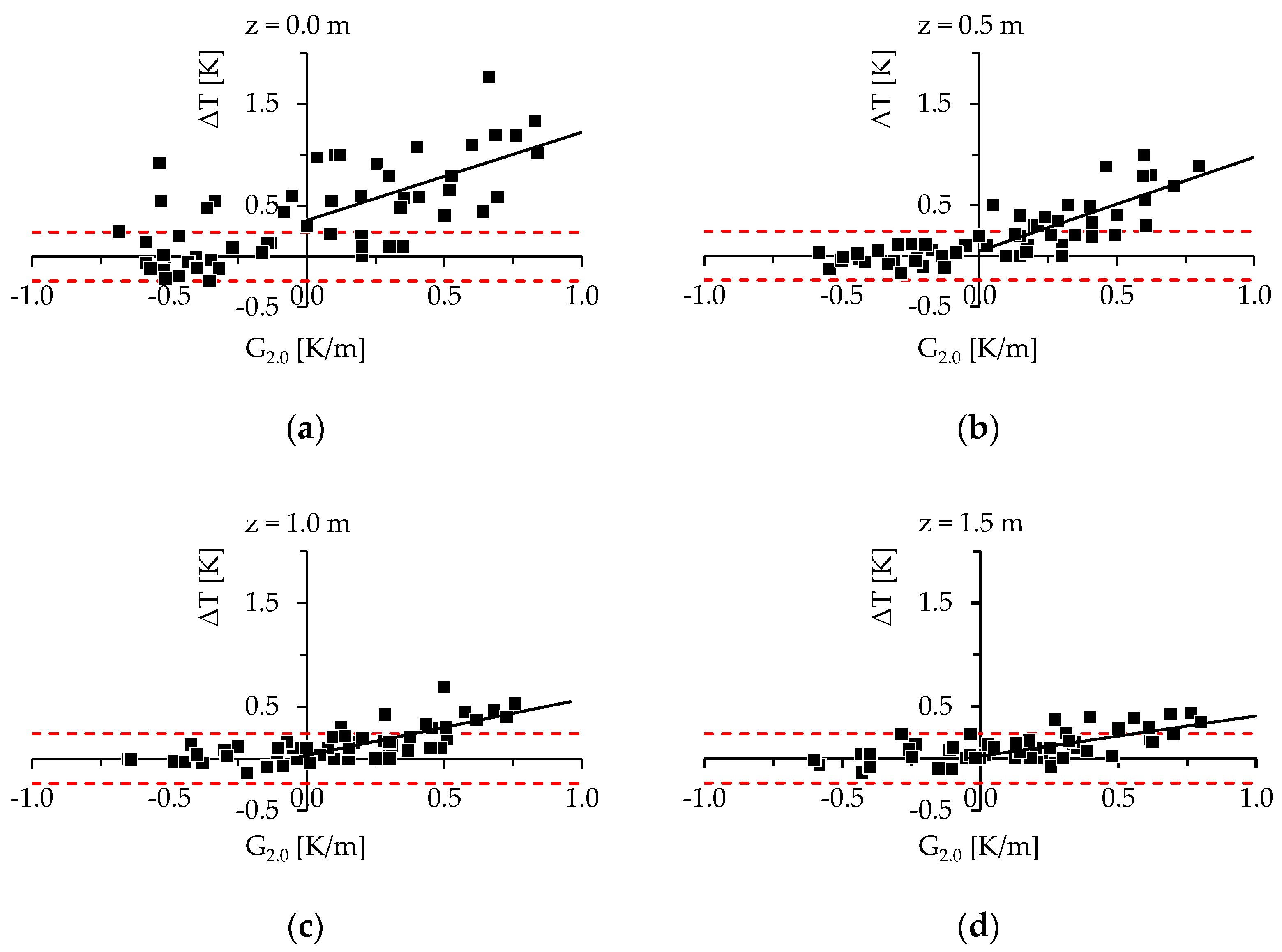
On the simplifying assumption that G2.0 and ΔT correlate linearly, the Pearson coefficient (r) was calculated for each depth and each borehole (Table 3). As natural convection only starts when a critical positive thermal gradient is exceeded, only thermal gradients of G2.0 ≥ 0.0 m/K were considered. As can be seen in Table 3, clear correlations (r ≥ 0.5) are found in each borehole at at least two depths. In the boreholes B3, B4, B5 and B6, r coefficients ≥ 0.8 occurred.
When all of the values at each step were included, a significant and clear correlation was found at z = 0.0 m (r = 0.5) and at z = 0.5–1.5 m (r = 0.7). Using linear regression, it is possible to determine the threshold thermal gradient (Gt) for all boreholes and depths for which ΔT > 0.2 K. When all of the data are considered, the threshold thermal gradient Gt lies between 0.3 K/m and 0.4 K/m. Some values of Gt deviate significantly from these values, with the largest maximum value of Gt (0.8 K/m) found in B3 at z = 1.5 m.
4. Discussion
4.1. Deviations of GWT from the Ambient Subsurface Temperature in MWs
Measured subsurface temperatures in TMSs show well-known temperature depth profiles with seasonal variations as described e.g., by Kurylyk et al. [49]. Similarly, seasonal shifts in the GWT were observed in all MWs. As described above, the natural thermal conditions within the subsurface of the test site are assumed to be disturbed due to operational and leak testing of the LSC. At approximately 10 m below ground level, small temperature fluctuations were still present, except in borehole B6, thus the neutral zone had not yet been reached at this depth. The neutral zone is the subsurface zone that is no longer thermally influenced by the climate at the surface; it is normally located at depths of 10 m or more [10].
As the maximum thermal gradient observed in this study was G0.5 = 1.2 K/m, it was assumed that no significant natural convection occurred in the TMSs, particularly in the groundwater zone. According to Table 1, the simplified critical thermal gradient for natural convection in water columns with a diameter of 25 mm at a temperature of 10 °C is 1.3 K/m. The measured temperature can therefore be regarded as the actual temperature of the surrounding subsurface. For the measurements conducted in February, the TMSs had a diameter of 32 mm and thus a lower critical thermal gradient of 0.5 K/m. In February, this critical value was occasionally exceeded thus natural convection in the TMSs in February cannot be ruled out. However, due to the significantly smaller diameter of the water column in a TMS compared to a MW, it was assumed that natural convection had significantly less effects on the temperature measurements in TMSs than in MWs.
According to Figure 3, there are three significant areas in the water column with clusters of ΔT > 0.2 K. The possible causes for these temperature deviations will be discussed in detail in Section 4.2 and Section 4.3. Area A occurred in all boreholes down to a depth of 1.5 m below groundwater level and is primarily caused by thermal convection. The deviations in Area B and Area C are also mainly caused by convection. Area D was observed only in borehole B3. Here, forced convection creates a downward flow leading to GWTs that are colder than the actual temperature of surrounding subsurface.
Transcurrent flow as a possible decisive cause for temperature deviations in screened MWs can be ruled out. The groundwater flow direction in the shallow area is determined by the gaining stream “Usa” east of the test site. Therefore—in a large-scale consideration—a one-dimensional flow direction was predominantly assumed, especially for the shallow groundwater in the bench gravels.
4.2. Impact of Forced Convection on GWT Measurements
Between March and July, rapid temperature jumps were observed in the MW in borehole B3 in the depth-range 7.3–7.6 m below ground level. The GWT was up to 0.8 K colder than in the subsurface above where the temperature jumps occurred. The electrical conductivity of the groundwater was also found to increase in the same depth range as the jumps in the GWT. At this depth, beneath a thin layer of confining clay, the geological unit comprises silt with stony basalt components. Deeper down, below the bottom of the MW, the crumbly basalt was found to be water-bearing while drilling. The increased electrical conductivity measured at this depth indicates that the silt with stony basalt components is permeable to a certain extent and is at least temporarily water-bearing and of higher salinity. Higher values of EC in the subsurface in Bad Nauheim have already been reported [50].
Because GWT was colder above the depths in which the temperature jumps were measured, natural convection due to a positive thermal gradient can be ruled out as the cause. Furthermore, the greater salinity and thus higher density of the deeper groundwater would impede natural convection [35]. As the increasing EC values showed at least temporary correlation with the observed temperature jumps, pollution can also be excluded as a cause.
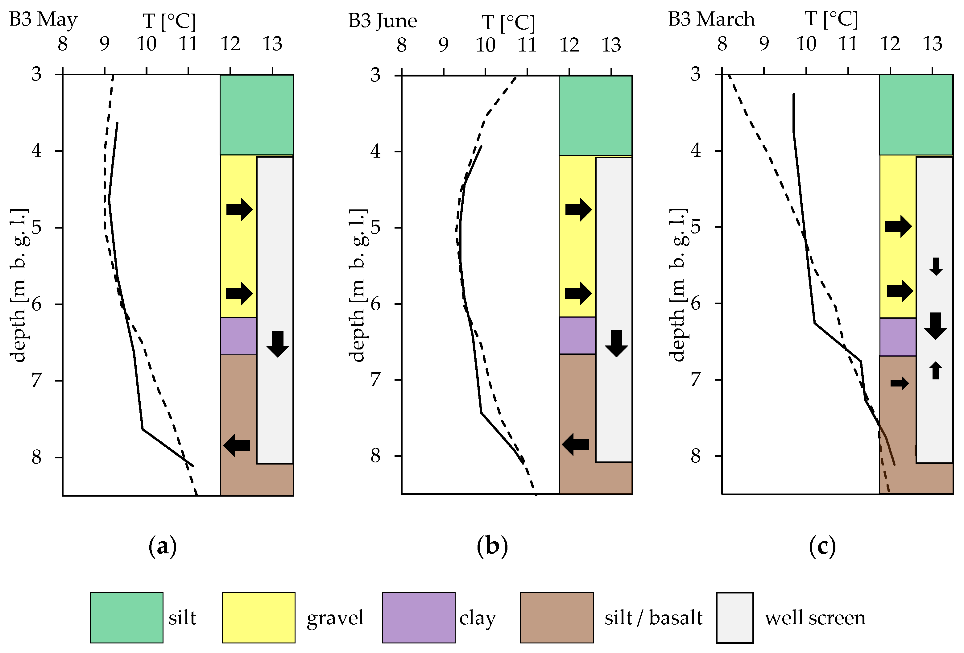
According to Berthold and Börner [35], vertical downward flows within MWs in combination with a positive downward thermal gradient leads to local GWTs that are colder than the ambient surface temperature. As can be seen in Figure 8, the negative temperature deviations observed from April to July can also be explained by downward flow in the MW. In this case, groundwater flows from the bench gravel into the MW and flows out again at the deeper decomposed basalt layer, where salinity is higher. Due to a positive thermal gradient between the in- and outflow sections of the well, colder GWTs are measured.
In March, another conductivity and temperature jump in the depth range 6.3–6.8 m below ground level was observed. At this time of the year, Area D was located in the gravel aquifer. This can be explained by assuming a temporary and less pronounced upward flow from the decomposed basalt within the MW. The positive but non-significant ΔT below Area D combined with a negative thermal gradient in October also suggest that there is a temporary upward flow in the lower section of the MW. The positive deviations in the upper part of the water column (Area A) in March are caused by thermal convection, as described in the following section.
4.3. Impact of Thermal Convection on GWT Measurements
According to Table 1, the critical thermal gradient for natural convection to occur in water columns in MWs with a diameter of 80 mm is 0.01 K/m. As the downward positive thermal gradients nearly always exceeded this critical value, thermal convection was present in the MWs.
However, as EC gradients were detected that were equal to zero or were slightly negative in the downward direction, solutal convection could be ruled out as a decisive factor for vertical flow. In B3, vertical flow driven by forced convection was identified. The strongly increasing values of EC in the lower part of the water column also have a stabilising effect on natural convection.
Exclusively positive significant temperature deviations were found in Area A in each borehole. These deviations correlate well with the prevailing positive thermal gradients (G2.0), as can be seen in Figure 7 and Table 3. Furthermore, significant deviations associated with negative thermal gradients were observed in Area A at z = 0.0 m below groundwater level. An argument supporting the idea that these temperature deviations are caused by thermal convection is that they only arise when there are positive gradients and that we observed no significant negative deviations in combination with negative gradients. However, the presence of small-scale forced upward flows cannot be completely ruled out.
Significant deviations with negative gradients were measured sporadically at times of warm surface temperatures. These results can be explained if it is assumed that the probe of the TLC-meter was still warm (as a result of the higher surface air temperatures) when inserted and this affected the temperature measurement at the groundwater table. The lower Pearson coefficient for z = 0.0 m can therefore be explained. The material of the well casing itself has no influence on the subsurface temperature [8].
Just as with Area A, the deviations in Area B also occurred with positive thermal gradients and can thus be explained by thermal convection. These deviations occurred in combination with a positive thermal gradient in Area B, but with a locally negative gradient or gradient equal to zero in Area A. This was particularly observed in borehole B5 in the period May–July (Figure 5c). Similarly, the significant negative temperature deviations in Area C are accompanied by positive thermal gradients in the lower part of the water column. From this, it is deduced, that colder water sinks due to thermal convection leading to the observed negative temperature deviation. The effects of thermal convection and forced convection observed in this study are shown for each borehole in Figure 9.
In thermal convection, water circulates due to density differences in the section of the water column in which there is a downward positive thermal gradient [35]. In wells with diameters of 4.8 cm, these convection cells can extend up to 0.5 m in height and they can reach even higher in larger diameter wells [41]. The fact that the thermally driven deviations are greatest in the vicinity of the groundwater table and that they decrease with depth can be explained by the fact that a sort of stack of convection cells forms and warmer water is transported upwards within the MW via these convection cells. In the middle of the water column, the temperature is stabilised by convection cells above and below this zone, at least within the accuracy levels applicable to field-based temperature measurements. This is also the reason why the deviations in Area B only occur with negative gradients or gradients equal to zero in the upper area. Correspondingly, cold water is transported downwards through the pile of convection cells, resulting in negative deviations at the lower end of the water column with a positive gradient. In the middle of the water column, the inflow of groundwater through the well screen may also provide additional temperature stabilisation.
The deviations are greatest in the upper part of the water column where there are greater thermal gradients due to the shorter distance to the surface. These deviations are therefore of particular importance for evaluating GWT measurements in practice. Therefore, the threshold thermal Gt, above which significant temperature deviations (ΔT > 0.2 K) are likely to occur in the upper part of the water column, was calculated for MWs with a diameter of 80 mm. However, as can be seen in Table 3, there are significant differences in Gt between boreholes, thus this should only be considered as a rough guide. In general, for thermal gradients of 0.3 K/m, the possibility of temperature deviations should be considered when evaluating GWT measurements. Since thermal convection in a water column is also dependent on the diameter, a lower value of Gt can be expected for larger diameter columns.
These threshold thermal gradients are mainly reached during the cold season, but the distance from the groundwater level to the surface must also be considered. At greater depths, these threshold thermal gradients will be observed delayed, thus positive thermal gradients can also occur in the warmer season (Area B). Similarly, a cooling of the shallow subsurface, e.g., due to geothermal use, can be expected to increase the thermal gradient.
4.4. Recommended Monitoring Concept for LSCs
LSCs, as described by Zeh et al. [28], have not found widespread use thus far. However, as these systems extract heat or cold from the very shallow subsurface over a large area, groundwater monitoring should be installed to observe the thermal impact of the system, especially when groundwater-to-surface distances are small. This type of monitoring is already being carried out for other geothermal systems. The normal method of measuring GWT involves the use of screened MWs. In view of the results from this study, the question arises as to which kind of well casing should be used in order to obtain temperature measurements of sufficient accuracy.
Climate conditions at the surface continue to influence the temperature in the subsurface down to depths of 10–15 m [10]. This results in larger thermal gradients. Due to these larger positive thermal gradients, temperature deviations caused by thermal convection become more prevalent. When heat is extracted from the subsurface, due to the presence of an LSC, these positive thermal gradients can become even larger.
In this study, deviations up to 1.8 K at the groundwater table and 1.0 K at 0.5 m below groundwater level were measured in screened MWs due to thermal convection. With larger diameters or different thermal conditions, temperature deviations can be even higher [41,45]. Given the permissible temperature differences for (open) shallow geothermal systems of ±6 K in Germany or ±3 K in Switzerland [34], these deviations can be crucial when evaluating GWT measurements. This could, for instance, result in an incorrect measurement of the cooling of very shallow groundwater.
In light of these findings, MWs with very small diameters, such as piezometers, are more suitable, as they significantly reduced the effects of thermal convection. However, forced convection due to existing well screens is still possible. The effects of forced convection can be reduced by reducing the length of screen. To reduce the effects of natural convection and to fully prevent forced convection, TMS well casings with no screen and with small diameters can be used. In addition, the temperature of the unsaturated zone can also be measured. However, these systems provide no information on the groundwater level. Well screens are also required in order to carry out groundwater sampling, e.g., for groundwater quality monitoring as recommend by Hähnlein et al. [34], or to perform hydraulic aquifer tests such as pumping tests.
For GWT monitoring at LSC sites the configuration used in this study, i.e., the combination of a TMS and an MW installed in a single borehole, is generally recommended. As this does not increase the number of required boreholes, it also helps to limit additional costs. However, the monitoring concept should always be adapted to the conditions on site and the specific water management requirements. In particular, the effects of forced convection or solutal convection are strongly dependent on the local hydrogeological conditions. Finally, it should be noted that even when using the variant proposed here with a combination of MWs and TMSs, convection processes may still occur due to filling of the borehole with filter gravel, which can lead to temperature deviations in the TMS itself.
The advantages offered by different well casings in boreholes for monitoring of very shallow geothermal systems are summarised in Table 4.
Natural convection currents can also be prevented through other methods. For example, well fillers with lower viscosity can be used [45]. If these can be removed from the well by purging, pumping tests and sampling can also be carried out.
5. Conclusions
From February to October 2021, temperature measurements were conducted in groundwater monitoring wells and in water-filled well-casings without screens, each installed in a single borehole. Comparison of the temperature–depth profiles show that the temperatures measured in the monitoring wells differ from those recorded in the TMSs. In the upper water column of the MWs groundwater temperatures that measured up to 1.8 K warmer were observed. These observed temperature deviations correlate clearly to the thermal gradient. It was concluded that the deviations were driven by natural thermal convection currents. As an initial benchmark for guidance purposes, significant temperature deviations in the upper part of the water column can be expected when the thermal convection gradient is 0.3 K/m or higher.
As the critical gradient for natural convection in the TMSs was not reached, the water column in these measuring systems can be considered to be stable and to represent the prevailing thermal conditions in the surrounding bedrock. Other temperature deviations observed in the monitoring wells were attributed either to natural convection or to forced convection in the wells. In B3, this resulted in groundwater temperatures that measured up to 0.8 K colder due to the downward flow of the groundwater. This vertical flow was caused by different hydraulic heads in permeable layers, which were separated by a non-permeable clay layer, within the well screen section.
As the installation of large-scale geothermal collector systems would lead to greater cooling in the shallow subsurface zone, which would intensify the downward positive thermal gradient, increases in temperature deviations of monitoring wells are to be expected. It is therefore recommended that, depending on the specific requirements of the water management monitoring programme, a combination of monitoring wells and non-screened well casings with small diameters should be used in order to obtain reliable temperature measurements while also allowing for further hydraulic investigations or groundwater sampling.
Author Contributions
Conceptualization, M.R.; methodology, M.R.; validation, M.R.; formal analysis, M.R.; investigation, M.R.; resources, D.B. and M.R.; data curation, M.R.; writing—original draft preparation, M.R. and D.B.; writing—review and editing, M.R. and D.B.; visualization, M.R.; supervision, D.B.; project administration, D.B. and M.R.; funding acquisition, D.B. All authors have read and agreed to the published version of the manuscript.
Funding
This research was funded in the cause of ‘KNW-Opt’ by Federal Ministry for Economic Affairs and Climate Action (BMWK), Grant No. 03EN3020C.
Data Availability Statement
The data presented in this study are available on request from the corresponding author. The data are not publicly available due to privacy restrictions.
Acknowledgments
We would like to thank and express great gratitude to our research partners Stockinger and his group from the Technische Hochschule Nürnberg as well as to Stadtwerke Bad Nauheim GmbH, who provided administrative support during our measurements. We also thank the members of the shallow geothermal working group at Friedrich-Alexander Universität Erlangen-Nürnberg for their help with the measurements and valuable discussions. Last but not least, we would like to thank our colleagues from Rohn’s engineering geology working group (FAU) for providing the TLC-meter.
Conflicts of Interest
The authors declare no conflict of interest.
References
- Farouki, O.T. Thermal Properties of Soils; Cold Regions Research and Engineering Lab Hanover NH: Hanover, NH, USA, 1981. [Google Scholar]
- Bertermann, D.; Klug, H.; Morper-Busch, L.; Bialas, C. Modelling vSGPs (very shallow geothermal potentials) in selected CSAs (case study areas). Energy 2014, 71, 226–244. [Google Scholar] [CrossRef]
- Bertermann, D.; Schwarz, H. Laboratory device to analyse the impact of soil properties on electrical and thermal conductivity. Int. Agrophys. 2017, 31, 157–166. [Google Scholar] [CrossRef] [Green Version]
- Di Sipio, E.; Bertermann, D. Factors Influencing the Thermal Efficiency of Horizontal Ground Heat Exchangers. Energies 2017, 10, 1897. [Google Scholar] [CrossRef] [Green Version]
- Di Sipio, E.; Bertermann, D. Thermal properties variations in unconsolidated material for very shallow geothermal application (ITER project). Int. Agrophys. 2018, 32, 149–164. [Google Scholar] [CrossRef]
- Schwarz, H.; Bertermann, D. Mediate relation between electrical and thermal conductivity of soil. Géoméch. Geophys. Geo-Energy Geo-Resour. 2020, 6, 50. [Google Scholar] [CrossRef]
- Xu, X.; Zhang, W.; Fan, C.; Li, G. Effects of temperature, dry density and water content on the thermal conductivity of Genhe silty clay. Results Phys. 2020, 16, 102830. [Google Scholar] [CrossRef]
- Alexander, M.D.; MacQuarrie, K.T.B. The measurement of groundwater temperature in shallow piezometers and standpipes. Can. Geotech. J. 2005, 42, 1377–1390. [Google Scholar] [CrossRef]
- Huber, H.; Arslan, U.; Sass, I. Zum Einfluss der Filtergeschwindigkeit des Grundwassers auf die effektive Wärmeleitfähigkeit. Grundwasser 2014, 19, 173–179. [Google Scholar] [CrossRef]
- Taylor, C.A.; Stefan, H.G. Shallow groundwater temperature response to climate change and urbanization. J. Hydrol. 2009, 375, 601–612. [Google Scholar] [CrossRef]
- Benz, S.A.; Bayer, P.; Winkler, G.; Blum, P. Recent trends of groundwater temperatures in Austria. Hydrol. Earth Syst. Sci. 2018, 22, 3143–3154. [Google Scholar] [CrossRef] [Green Version]
- Gunawardhana, L.N.; Kazama, S. Climate change impacts on groundwater temperature change in the Sendai plain, Japan. Hydrol. Process. 2011, 25, 2665–2678. [Google Scholar] [CrossRef]
- Hemmerle, H.; Bayer, P. Climate Change Yields Groundwater Warming in Bavaria, Germany. Front. Earth Sci. 2020, 8, 575894. [Google Scholar] [CrossRef]
- Menberg, K.; Bayer, P.; Zosseder, K.; Rumohr, S.; Blum, P. Subsurface urban heat islands in German cities. Sci. Total Environ. 2013, 442, 123–133. [Google Scholar] [CrossRef] [PubMed]
- Schweighofer, J.A.V.; Wehrl, M.; Baumgärtel, S.; Rohn, J. Detecting Groundwater Temperature Shifts of a Subsurface Urban Heat Island in SE Germany. Water 2021, 13, 1417. [Google Scholar] [CrossRef]
- Tissen, C.; Benz, S.A.; Menberg, K.; Bayer, P.; Blum, P. Groundwater temperature anomalies in central Europe. Environ. Res. Lett. 2019, 14, 104012. [Google Scholar] [CrossRef] [Green Version]
- Zhu, K.; Bayer, P.; Grathwohl, P.; Blum, P. Groundwater temperature evolution in the subsurface urban heat island of Cologne, Germany. Hydrol. Process. 2015, 29, 965–978. [Google Scholar] [CrossRef]
- Vienken, T.; Händel, F.; Epting, J.; Dietrich, P.; Liedl, R.; Huggenberger, P. Energiewende braucht Wärmewende–Chancen und Limitierungen der intensiven thermischen Nutzung des oberflächennahen Untergrundes in urbanen Gebieten vor dem Hintergrund der aktuellen Energiedebatte in Deutschland. Grundwasser 2016, 21, 69–73. [Google Scholar] [CrossRef]
- Hähnlein, S.; Molina-Giraldo, N.; Blum, P.; Bayer, P.; Grathwohl, P. Ausbreitung von Kältefahnen im Grundwasser bei Erdwärmesonden. Grundwasser 2010, 15, 123–133. [Google Scholar] [CrossRef]
- Steiner, C.; Heimlich, K.; Hilberg, S. Vergleichende Temperaturfahnenprognose anhand zweier industriell genutzter Grundwasserwärmepumpen: FEFLOW vs. ÖWAV-Modell. Grundwasser 2016, 21, 173–185. [Google Scholar] [CrossRef] [Green Version]
- Vienken, T.; Kreck, M.; Dietrich, P. Monitoring the impact of intensive shallow geothermal energy use on groundwater temperatures in a residential neighborhood. Geotherm. Energy 2019, 7, 8. [Google Scholar] [CrossRef]
- Fuji, H.; Tsuya, S.; Harada, R.; Kosukegawa, H. Field Test of Horizontal Ground Heat Exchangers Installed Using Horizontal Directional Drilling Technology. In Proceedings of the 44th Workshop on Geothermal Reservoir Engineering, Stanford, CA, USA, 11–13 February 2019. [Google Scholar]
- Fuji, H.; Yamasaki, S.; Maehara, T. Numerical modeling of slinky-coil horizontal ground heat exchangers considering snow coverage effects. In Proceedings of the Thirty-Eighth Workshop on Geothermal Reservoir Engineering, Stanford, CA, USA, 11–13 February 2013. [Google Scholar]
- Ramming, K. Bewertung und Optimierung Oberflächennaher Erdwärmekollektoren für Verschiedene Lastfälle. Ph.D. Thesis, Technische Universität Dresden, Dresden, Germany, 2007. [Google Scholar]
- Sangi, R.; Müller, D. Dynamic modelling and simulation of a slinky-coil horizontal ground heat exchanger using Modelica. J. Build. Eng. 2018, 16, 159–168. [Google Scholar] [CrossRef]
- Selamat, S.; Miyara, A.; Kariya, K. Analysis of Short Time Period of Operation of Horizontal Ground Heat Exchangers. Resources 2015, 4, 507–523. [Google Scholar] [CrossRef] [Green Version]
- Wu, Y.; Gan, G.; Verhoef, A.; Vidale, P.L.; Gonzalez, R.G. Experimental measurement and numerical simulation of horizontal-coupled slinky ground source heat exchangers. Appl. Therm. Eng. 2010, 30, 2574–2583. [Google Scholar] [CrossRef] [Green Version]
- Zeh, R.; Ohlsen, B.; Philipp, D.; Bertermann, D.; Kotz, T.; Jocic, N.; Stockinger, V. Large-Scale Geothermal Collector Systems for 5th Generation District Heating and Cooling Networks. Sustainability 2021, 13, 6035. [Google Scholar] [CrossRef]
- Arning, E.; Kölling, M.; Schulz, H.D.; Panteleit, B.; Reichling, J. Einfluss oberflächennaher Wärmegewinnung auf geochemische Prozesse im Grundwasserleiter. Grundwasser 2006, 11, 27–39. [Google Scholar] [CrossRef]
- Bonte, M.; van Breukelen, B.M.; Stuyfzand, P.J. Temperature-induced impacts on groundwater quality and arsenic mobility in anoxic aquifer sediments used for both drinking water and shallow geothermal energy production. Water Res. 2013, 47, 5088–5100. [Google Scholar] [CrossRef]
- Brielmann, H.; Lueders, T.; Schreglmann, K.; Ferraro, F.; Avramov, M.; Hammerl, V.; Blum, P.; Bayer, P.; Griebler, C. Oberflächennahe Geothermie und ihre potenziellen Auswirkungen auf Grundwasserökosysteme. Grundwasser 2011, 16, 77–91. [Google Scholar] [CrossRef]
- Griebler, C.; Brielmann, H.; Haberer, C.; Kaschuba, S.; Kellermann, C.; Stumpp, C.; Hegler, F.; Kuntz, D.; Walker-Hertkorn, S.; Lueders, T. Potential impacts of geothermal energy use and storage of heat on groundwater quality, biodiversity, and ecosystem processes. Environ. Earth Sci. 2016, 75, 1391. [Google Scholar] [CrossRef]
- VDI. VDI 4640 Part 1. Thermal Use of the Underground Fundamentals, Approvals, Environmental Aspects; Beuth Verlag GmbH: Berlin, Germany, 2010. [Google Scholar]
- Hähnlein, S.; Bayer, P.; Ferguson, G.; Blum, P. Sustainability and policy for the thermal use of shallow geothermal energy. Energy Policy 2013, 59, 914–925. [Google Scholar] [CrossRef]
- Börner, F.; Berthold, S. Vertical flows in groundwater monitoring wells. In Groundwater Geophysics; Kirsch, R., Ed.; Springer: Berlin/Heidelberg, Germany, 2009; pp. 367–389. [Google Scholar]
- Church, P.E.; Granato, G.E. Bias in Ground-Water Data Caused by Well-Bore Flow in Long-Screen Wells. Groundwater 1996, 34, 262–273. [Google Scholar] [CrossRef]
- Elçi, A.; Flach, G.; Molz, F. Detrimental Effects of Natural Vertical Head Gradients on Chemical and Water Level Measurements in Observation Wells: Identification and Control. J. Hydrol. 2003, 281, 70–81. [Google Scholar] [CrossRef]
- Berthold, S.; Börner, F. Detection of free vertical convection and double-diffusion in groundwater monitoring wells with geophysical borehole measurements. Environ. Geol. 2008, 54, 1547–1566. [Google Scholar] [CrossRef]
- Diment, W.H. Thermal Regime of a Large Diameter Borehole: Instability Of The Water Column And Comparison Of Air- And Water-filled Conditions. Geophysics 1967, 32, 720–726. [Google Scholar] [CrossRef]
- Krige, L.J. Borehole temperatures in the Transvaal and Orange Free State. Proc. R. Soc. Lond. 1939, 173, 450–474. [Google Scholar] [CrossRef] [Green Version]
- Sammel, E.A. Convective flow and its effect on temperature logging in small-diameter wells. Geophysics 1968, 33, 1004–1012. [Google Scholar] [CrossRef]
- Rayleigh, L. LIX. On convection currents in a horizontal layer of fluid, when the higher temperature is on the under side. Lond. Edinb. Philos. Mag. J. Sci. 1916, 32, 529–546. [Google Scholar] [CrossRef] [Green Version]
- Gershuni, G.Z.; Zhukhovitskii, E.M. Convective Stability of Incompressible Fluids; Keter Publishing House Jerusalem Ltd.: Jerusalem, Israel, 1976. [Google Scholar]
- Berthold, S.; Resagk, C. Investigation of thermal convection in water columns using particle image velocimetry. Exp. Fluids 2012, 52, 1465–1474. [Google Scholar] [CrossRef]
- Eppelbaum, L.; Kutasov, i. Estimation of the effect of thermal convection and casing on the temperature regime of boreholes: A review. J. Geophys. Eng. 2011, 8, R1–R10. [Google Scholar] [CrossRef]
- Kümmerle, E. Geologische Karte von Hessen 1:25,000 5618 Friedberg; Hessisches Landesamt Für Bodenforschung: Wiesbaden, Germany, 1976. [Google Scholar]
- Hölting, B.; Coldewey, W.G. Hydrogeology, 1st ed.; Springer: Berlin/Heidelberg, Germany, 2019; p. 357. [Google Scholar]
- Kümmerle, E. Erläuterungen zur Geologischen Karte von Hessen 1:25,000: Blatt Nr. 5618 Friedberg; Hessisches Landesamt für Bodenforschung: Wiesbaden, Germany, 1976; p. 247. [Google Scholar]
- Kurylyk, B.; Macquarrie, K.; Caissie, D.; McKenzie, J. Shallow groundwater thermal sensitivity to climate change and land cover disturbances: Derivation of analytical expressions and implications for stream temperature modeling. Hydrol. Earth Syst. Sci. 2015, 19, 2469–2489. [Google Scholar] [CrossRef] [Green Version]
- Schäffer, R.; Sass, I. Ausbreitung und Vermischung geogener, kohlendioxidführender Thermalsole in oberflächennahem Grundwasser, Bad Nauheim. Grundwasser 2016, 21, 305–319. [Google Scholar] [CrossRef]
- Chen, W.; Bense, V. Using transient temperature–depth profiles to assess vertical groundwater flow across semi-confining layers in the Chianan coastal plain aquifer system, southern Taiwan. Hydrogeol. J. 2019, 27, 2155–2166. [Google Scholar] [CrossRef]
- Constantz, J.; Tyler, S.W.; Kwicklis, E. Temperature-Profile Methods for Estimating Percolation Rates in Arid Environments. Vadose Zone J. 2003, 2, 12–24. [Google Scholar] [CrossRef]
- Taniguchi, M. Estimated Recharge Rates from Groundwater Temperatures In The Nara Basin, Japan. Appl. Hydrogeol. 1994, 2, 7–14. [Google Scholar] [CrossRef]
- Taniguchi, M.; Turner, J.V.; Smith, A.J. Evaluations of groundwater discharge rates from subsurface temperature in Cockburn Sound, Western Australia. Biogeochemistry 2003, 66, 111–124. [Google Scholar] [CrossRef]
- Doussan, C.; Toma, A.; Poitevin, G.; Ledoux, E.; Detay, M. Coupled use of thermal and hydraulic head data to characterize river-groundwater exchanges. J. Hydrol. 1994, 153, 215–229. [Google Scholar] [CrossRef]
- Hunt, R.J.; Krabbenhoft, D.P.; Anderson, M.P. Groundwater inflow measurements in wetland systems. Water Resour. Res. 1996, 32, 495–507. [Google Scholar] [CrossRef]
- Land, L.A.; Paull, C.K. Thermal gradients as a tool for estimating groundwater advective rates in a coastal estuary: White Oak River, North Carolina, USA. J. Hydrol. 2001, 248, 198–215. [Google Scholar] [CrossRef]
Figure 1.
(a) Large-scale geothermal collector system (LSC) and positioning of six boreholes around the LSC site; (b) each borehole contains a groundwater monitoring well (MW) and a temperature measuring station (TMS). Additionally shown are the well casings, the borehole filling, the boundaries of the geological units in metres below ground level (m b. g. l) and the mean groundwater level in each borehole. For ease of representation, the overlying soils have been combined with the loamy valley deposits. In the deepest section of each borehole, the drill diameter was reduced from 220 mm to 178 mm, which is not shown in the figure.

Figure 2.
Examples of temperature (T) depth profiles in selected boreholes; (a) MW in B1; (b) MW in B3; (c) MW in B6; (d) TMS in B1; (e) TMS in B3; (f) TMS in B6.
Figure 2.
Examples of temperature (T) depth profiles in selected boreholes; (a) MW in B1; (b) MW in B3; (c) MW in B6; (d) TMS in B1; (e) TMS in B3; (f) TMS in B6.

Figure 3.
Values of ΔT for all boreholes; (a) B1; (b) B2; (c) B3; (d) B4; (e) B5 and (f) B6. The area within the dashed red lines indicates the measurement accuracy of the TLC-meter (ΔT ≤ 0.2 K). Temperature differences outside of the dashed lines are considered significant. Areas with clusters of significant ΔT values (areas A, B, C and D), as described in the text, are marked.

Figure 4.
Measured electrical conductivities (EC) of groundwater in selected boreholes; (a) B2; (b) B3; (c); B5.
Figure 4.
Measured electrical conductivities (EC) of groundwater in selected boreholes; (a) B2; (b) B3; (c); B5.

Figure 5.
Main soil types and hard rock types in borehole B3 and the measured values of ΔT and EC at selected measuring times; (a) March; (b) April; (c) June. For ease of representation, interjacent silt layers in the bench gravel were neglected.
Figure 5.
Main soil types and hard rock types in borehole B3 and the measured values of ΔT and EC at selected measuring times; (a) March; (b) April; (c) June. For ease of representation, interjacent silt layers in the bench gravel were neglected.

Figure 6.
Thermal gradients (G0.5) between each measuring step of 0.5 m for selected boreholes; (a) B1; (b) B4; (c) B6.
Figure 6.
Thermal gradients (G0.5) between each measuring step of 0.5 m for selected boreholes; (a) B1; (b) B4; (c) B6.

Figure 7.
Correlation between ΔT and the thermal gradient interpolated over a distance of 2 m at a certain depth (G2.0) and the linear regression for G2.0 ≥ 0.0 m/K; (a) z = 0.0 m; (b) z = 0.5 m; (c) z = 1.0 m; (d) z = 1.5 m. The area bounded by the dashed red lines represents the measurement accuracy of the TLC-meter (ΔT ≤ 0.2 K). Temperature differences outside of the dashed lines are considered significant.

Figure 8.
Temperature deviations in MWs due to forced convection. Temperature depth profiles MW (solid line) and surrounding subsurface (TMS, dashed line line) with main soil types and hard rock, flow directions from surrounding bedrock and within MW for selected measuring times based on schematic figures in Berthold and Börner [35]; (a) May; (b) June and (c) March. For ease of representation, interjacent silt layers in the bench gravel were neglected. Moreover, only flow directions caused by forced convection are shown.

Figure 9.
Temperature depth profiles in a MW and in surrounding subsurface and the dominant causes for temperature deviations: thermal convection (tc), forced convection (fc) or air temperature (at); (a) B1 in March; (b) B2 in April; (c) B3 in April; (d) B4 in March; (e) B5 in July; (f) B6 in April.


Table 1.
Critical thermal gradients for thermal convection in circular columns of pure water calculated for different monitoring well (MW) diameters and temperatures in accordance with Rayleigh [42] and Gershuni and Zhukhovitskii [43]. According to Börner and Berthold [35] a critical Rayleigh number of 148 is assumed.
| Diameter of MW [mm] | 5 °C | 10 °C | 15 °C | 20 °C | 25 °C | 30 °C |
|---|---|---|---|---|---|---|
| 25 | 11.02 | 1.26 | 0.64 | 0.42 | 0.31 | 0.24 |
| 50 | 0.69 | 0.08 | 0.04 | 0.03 | 0.02 | 0.01 |
| 80 | 0.11 | 0.01 | 0.01 | <0.01 | <0.01 | <0.01 |
| 100 | 0.0 | <0.01 | <0.01 | <0,01 | <0.01 | <0.01 |
| 125 | 0.02 | <0.01 | <0.01 | <0,01 | <0.01 | <0.01 |
Table 2.
Elevation at the location of the MWs and TMSs in metres above sea level (m a. s. l.), depth of bottom of MW and TMS, location of PVC well screen in the MWs, extent of geological units; ‘permeable basalt’ refers to areas where the decomposed basalt is presumed to be permeable, although it may not always be water-bearing.
| Borehole | Elevation [m a. s. l.] | Depth MW [m b. g. l] | Depth TMS [m b. g. l.] | Well Screen [m b. g. l] | Loam [m b. g. l.] | Gravel [m b. g. l.] | Permeable Basalt [m b. g. l.] |
|---|---|---|---|---|---|---|---|
| B1 | 142.5 | 10.1 | 10.4 | 6.1–10.1 | 0.8–6.4 | 6.4–8.5 | 10.0–10.5 |
| B2 | 141.3 | 10.0 | 10.3 | 6.0–10.0 | 0.8–4.6 | 4.6–7.3 | - |
| B3 | 139.9 | 8.1 | 10.4 | 4.1–8.1 | 0.8–4.1 | 4.1–6.2 | 6.7–10.5 |
| B4 | 139.5 | 10.0 | 10.3 | 5.0–10.0 | 1.3–3.5 | 3.5–7.8 | - |
| B5 | 139.2 | 10.1 | 10.3 | 5.1–10.1 | 0.8–3.3 | 3.3–5.8 | 6.9–10.4 |
| B6 | 138.7 | 6.0 | 10.3 | 4.0–6.0 | 0.3–3.1 | 3.1–5.5 | 8.1–10.5 |
Table 3.
Pearson’s coefficient (r) for the linear correlation between G2.0 and ΔT at different depths and for different boreholes and r is bold, when the p-value is less than or equal to the significance value of 5% and the correlation is thus significant. The table also lists the threshold gradient (Gt) above which ΔT is considered significant based on a linear regression analysis. In this study only values of G2.0 ≥ 0.0 m were used.
| z | B1 | B2 | B3 | B4 | B5 | B6 | Total | |||||||
|---|---|---|---|---|---|---|---|---|---|---|---|---|---|---|
| r | Gt | r | Gt | r | Gt | r | Gt | r | Gt | r | Gt | r | Gt | |
| 0.0 | 0.0 | - | 0.2 | - | 0.9 | 0.3 | 0.5 | 0.2 | 0.6 | 0.2 | 0.7 | 0.4 | 0.5 | 0.3 |
| 0.5 | 0.6 | 0.3 | 0.5 | 0.3 | 1.0 | 0.4 | 0.8 | 0.3 | 0.7 | 0.3 | 0.8 | 0.2 | 0.7 | 0.3 |
| 1.0 | 0.7 | 0.3 | 0.6 | 0.3 | 0.9 | 0.5 | 0.9 | 0.5 | 0.9 | 0.4 | 0.3 | - | 0.7 | 0.4 |
| 1.5 | 0.7 | 0.3 | −0.2 | - | 0.9 | 0.8 | 0.8 | 0.5 | 0.5 | 0.5 | 0.3 | - | 0.7 | 0.4 |
Table 4.
Benefits and possible investigations of different kinds of well casings; MW = monitoring well with a diameter ≥ 50 mm; PM = Piezometer (small diameter with filter screen); MW/TMS = monitoring well and temperature measuring station combined in one borehole; TMS = non-screened temperature measuring station with small diameter.
| Benefit of Specific Well Casing | MW | PM | TMS | MW/TMS |
|---|---|---|---|---|
| groundwater level | + | + | − | + |
| temperature in unsaturated zone | − | − | + | + |
| continuous temperatures with data logger | + | −/+ | + | + |
| minimised natural convection | − | + | + | + |
| no forced convection | − | −/+ | + | + |
| pumping tests or other hydraulic tests | + | − | − | + |
| groundwater sampling | + | − | − | + |
Publisher’s Note: MDPI stays neutral with regard to jurisdictional claims in published maps and institutional affiliations. |
© 2022 by the authors. Licensee MDPI, Basel, Switzerland. This article is an open access article distributed under the terms and conditions of the Creative Commons Attribution (CC BY) license (https://creativecommons.org/licenses/by/4.0/).
Share and Cite
MDPI and ACS Style
Bertermann, D.; Rammler, M. Suitability of Screened Monitoring Wells for Temperature Measurements Regarding Large-Scale Geothermal Collector Systems. Geosciences 2022, 12, 162. https://0-doi-org.brum.beds.ac.uk/10.3390/geosciences12040162
AMA Style
Bertermann D, Rammler M. Suitability of Screened Monitoring Wells for Temperature Measurements Regarding Large-Scale Geothermal Collector Systems. Geosciences. 2022; 12(4):162. https://0-doi-org.brum.beds.ac.uk/10.3390/geosciences12040162
Chicago/Turabian StyleBertermann, David, and Mario Rammler. 2022. "Suitability of Screened Monitoring Wells for Temperature Measurements Regarding Large-Scale Geothermal Collector Systems" Geosciences 12, no. 4: 162. https://0-doi-org.brum.beds.ac.uk/10.3390/geosciences12040162
Note that from the first issue of 2016, this journal uses article numbers instead of page numbers. See further details here.