1. Introduction
The Central Apennines are in the center of the Italian peninsula and consist of both the Umbria-Marche and the Abruzzi Mountain ranges. This mountain chain represents an Oligocene–Quaternary fold-and-thrust belt, resulting from the convergence of the African and European continental margins [
1,
2]. The area shows evidence of different deformation events, the last of which is responsible for the present-day seismicity of the area [
3,
4,
5,
6]. In the last 25 years, three different seismic sequences have affected this mountain group: Colfiorito (1997–1998), L’Aquila (2009), and the most recent one, Amatrice Visso-Norcia Campotosto (2016–2017). They have lasted for a long time with a series of moderate-to-large earthquakes distributed over 40 to 60 km-long Apenninic-trending segments [
7]. In this sense, the purpose of this paper is twofold: firstly, it aims to provide additional information and a geological interpretation of the seismic sequence after the 2016–2017 events. This was carried out by starting the analysis of the Global Navigation Satellite Systems (GNSS) data of more than 230 IGM95 geodetic network points and about 350 km of geometric leveling collected by the Italian Military Geographical Institute (IGM). Secondly, with the support of such a copious amount of new and accurate data, this allows for a precise geological interpretation of the events, both incorporating and confirming findings from published works and the existing literature. Therefore, the integration of prior studies in our paper serves two purposes: on the one hand, we reinforce what has already been achieved in existing research. On the other hand, it also shows how this study builds on existing works to advance concrete and up-to-date knowledge in the field.
The displacements of the Earth’s surface can be geodetically measured by several techniques, including triangulation with theodolites and/or Total Stations, GNSS, and remote sensing techniques, such as Differential Interferometric Synthetic Aperture Radar (DInSAR) and optical satellite imagery [
8].
This paper focuses on GNSS, which, according to recent literature, is currently employed worldwide for earthquake monitoring and prediction [
9,
10]. The Southern California Integrated GPS Network (SCIGN), a US Geological Survey Program presented by Hudnut et al. [
11] and whose goal is to monitor the state-of-the-art of 250 continuously operating stations, examines the ongoing crust deformation produced by the San Andreas fault and other tectonic elements in the Los Angeles Basin. Melbourne et al. [
12] describe the over 400 GNSS points of the combined PANGA (Pacific Northwest Geodetic Array) and PBO (Plate Boundary Observatory) networks operating along the Cascadia subduction zone; every point is telemetered in real-time and at a high rate. The availability of these permanent stations allowed for the application of novel approaches toward hazards mitigation since they monitor the M9 megathrust, the M7 crustal faults beneath population centers, several active Cascades volcanoes, and a host of other hazard sources. Hao et al. [
13] collected and processed three sources of GNSS datasets, including GNSS observations, GNSS positioning time series, and published GNSS velocities, to derive unified velocity and strain rate fields in East Asia. The VADASE (Variometric Approach for Standalone Engine Displacement Analysis) technique, applied to GNSS measurements, is used by [
14] to obtain displacements from seismic events with magnitudes on the Richter Scale (SR), greater than 7 and 9 occurred in the Indian Ocean (2016, 9.1 Mw), Chile (2010, 8.8 Mw) and New Zealand (2016, 7.8 Mw). In Italy, Anzidei et al. [
15], by comparing the pre- and post-earthquakes coordinates of the IGM95 and the Tyrgeonet networks, provide the estimation of the deformation associated with the seismic sequence that occurred in the Italian Umbria and Marche regions in 1997.
Moreover, the 2016–2017 coseismic sequence in Central Italy has already been studied by GNSS techniques [
16,
17]. The first authors used High-Rate sampling GNSS data from 52 permanent stations to retrieve the coseismic dynamic displacements, while the second authors, using low-cost GNSS receivers and short-baseline networks, presented a novel record of near-field coseismic displacement that was important for assessing fault displacement of surface ruptures, defining seismic hazard and predicting ground motion.
Other research focused on combining GNSS and DInSAR technologies [
18,
19,
20]. In fact, due to its high resolution and accuracy with extensive and continuous temporal coverage, DInSAR for surface displacement monitoring is widely used in earthquake investigations. Wang et al. [
18] have selected DInSAR and GNSS data to investigate the focal mechanism and the slip distribution of the Mw 6.4 earthquake that occurred in 2016 in Meinong (Taiwan, China). Belardinelli et al. [
19] have modelled the poroelastic signature of two medium-large earthquakes (Mw 6.1 and 6.0) that occurred in the Emilia-Romagna Region (Italy) in 2012 using both GNSS and DInSAR data. Niu et al. [
20] used GNSS data and C-band Radarsat-2 SAR imagery to map the coseismic surface deformation related to the 2014 Mw 6.1 Ludian County earthquake (Yunnan Province, China); after having inverted the derived coseismic deformation for the slip distribution based on the constructed conjugate fault model, they estimated the Coulomb failure stress due to the analyzed seismic event to investigate the potential seismic hazards in this region.
The results from DInSAR, also used to study the Amatrice earthquake in combination with GNSS data, allowed us to define a fairly coherent deformation pattern extended over the whole epicentral area [
21,
22,
23,
24,
25]. This data permitted us to characterize the deformation with pinpoint spatial and temporal accuracy, distinguish the coseismic deformation’s association with single main events of the sequence [
21,
22,
26], and measure the entire post-seismic deformation [
27]. Moreover, multitemporal data from radar interferometry was integrated with geological field data of surface coseismic ruptures [
28,
29,
30] and seismological data [
31] to analyze ground deformation and the triggered landslides to model the source geometry. Papadopoulos et al. [
32], based on rupture histories and DInSAR ground deformation model, the stress transfer among consecutive earthquake events from August to October 2016.
On the grounds of published geodetics works, other authors presented their geological interpretation and tectonic models of the 2016–2017 seismic sequence in Central Italy [
33,
34,
35,
36,
37,
38,
39].
Through GNSS surveys, the IGM, owner, and manager of the leading national geodetic networks updated the position of several geodetic points located close to the earthquake area after the 2016–2017 seismic sequence [
40]. The vertices belong to the IGM95 network [
41,
42], implemented in 1992 in parallel to the classic trigonometric networks; the network consists of 20,000 geodetic points (one every 20 km) endowed with individual monographies. The results of new measurements executed by IGM after the event and their comparison with previous data are described in this paper.
2. Geology of the Area
The study area, located in the central part of the Italian Apennine chain, results from different deformation events of the contractional and extensional types related to the convergence of African and European continental margins. This mechanism gave rise to a complex fold-and-thrust belt whose origin can be summarized in three principal tectonic phases [
43,
44]: first, a Jurassic extensional event, which caused the fragmentation of the carbonate platform in deep pelagic basins and shallow-water structural highs [
45]; a second late Miocene-early Pliocene NE verging compressional event, which caused the closure of the so-called Ligurian Ocean and the consequent continental collision generating the fold-and-thrust belt [
46]; a third late Pliocene-Quaternary extensional phase, which caused the developing of SW dipping, NNW-SSE trending normal fault systems (15 to 35 km-long) and, as a consequence, the development of several intramountain basins. This last phase is responsible for the present-day seismicity of the area, as shown by the occurrence of historical earthquakes [
47] and by the ongoing extensional deformation according to geodetic measurements at a medium rate of 3 mm/year [
48].
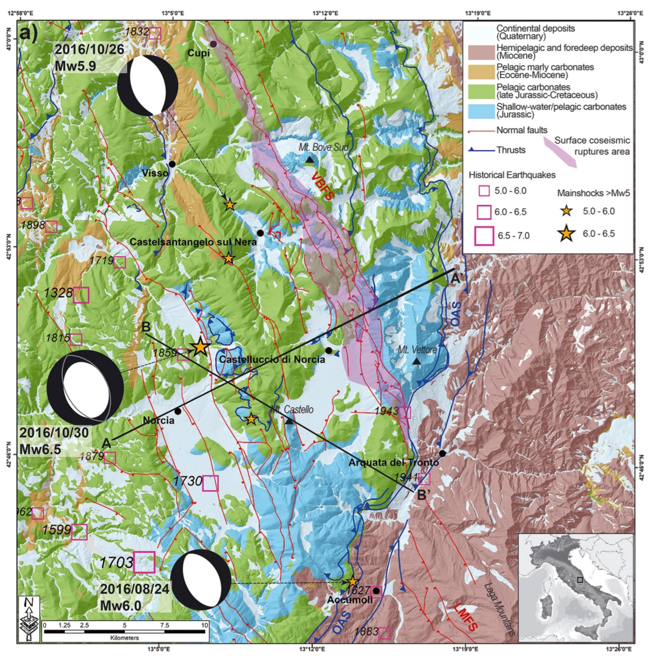
In the study area, there are two main extensional fault systems corresponding to the Mt. Vettore-Mt. Bove location (northern VBFS system in
Figure 1) and Mt. Laga (southern LMFS system in
Figure 1). VBFS is a roughly 30 km-long system composed of several NNW–SSE normal faults, both synthetic and antithetic, which affect the lower units of the Umbro-Marche domain and expose the Jurassic deposits at their footwall [
49]. The LMFS, comparable in size to the VBFS, comprises two main NW–SE fault segments affecting the weak Miocene Umbria-Marche units [
49,
50]. These two main systems, evidence of the actual extensional regime, are separated by a major regional curved-shape fold-and-thrust system that originated during the compressional phase. This structure, called Olevano-Antrodoco-Sibillini thrust (OAS in
Figure 1), superimposed the Meso-Cenozoic carbonatic multilayer over a wide Miocene foredeep basin, which was subject to a 10 km shortening [
51,
52]. The OAS changes its direction indicatively between Norcia and Amatrice and, therefore, in the central part of the study area, it becomes oblique to VBFS and LMFS. The importance of the OAS on the seismicity of the area may be decisive, controlling the evolution of the seismic activity. In fact, different authors have already studied how pre-existing structures can affect the evolution of Quaternary active fault systems acting as barriers [
6,
53,
54]. There is still debate among the scientific community about this interpretation. Still, recent studies on the 2016 central Italy earthquakes revealed the presence of barriers controlling the evolution of the seismic sequence [
22,
30,
35,
37,
38].
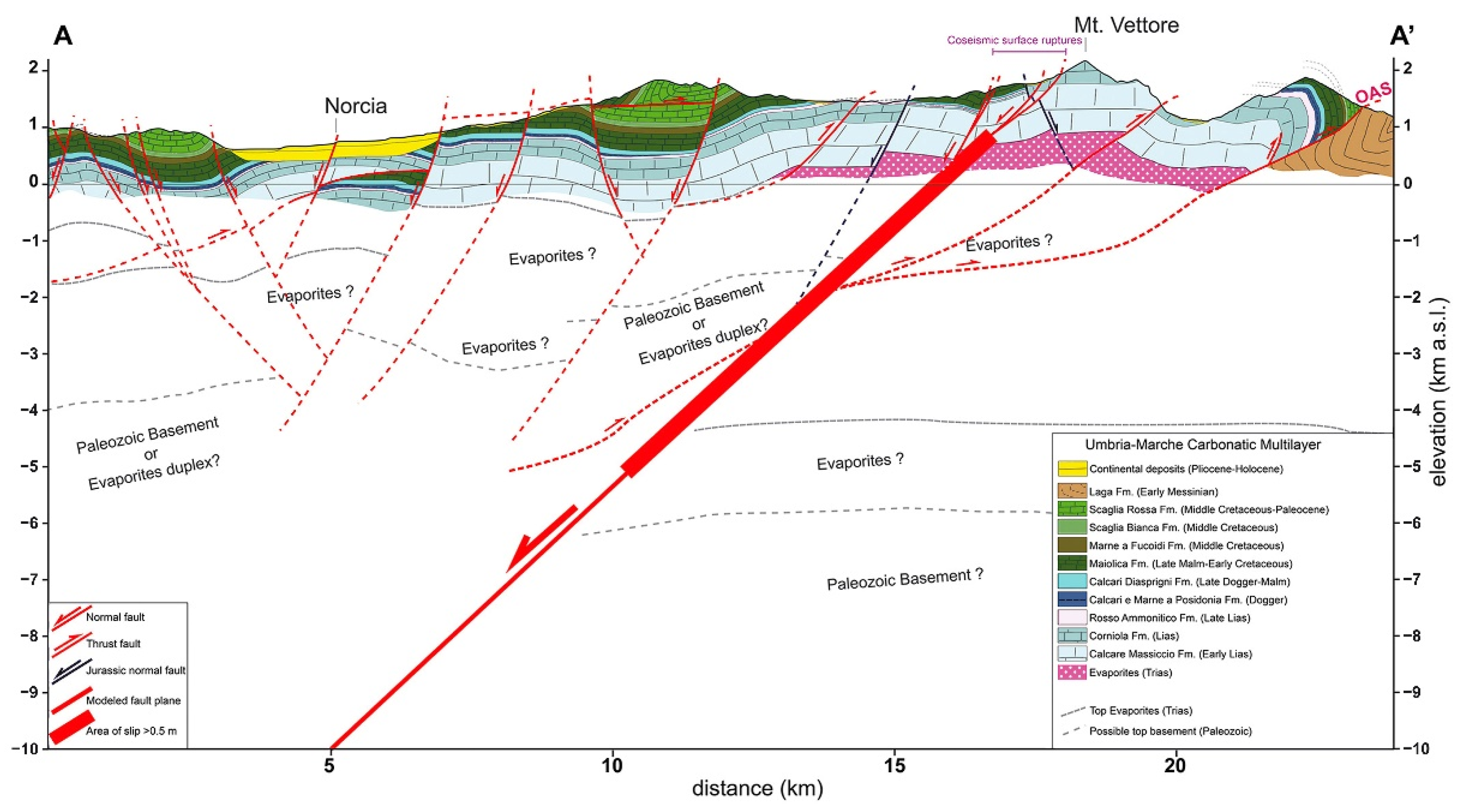
The A–A’ geological cross-section of
Figure 1 is shown in
Figure 2, where the Meso-Cenozoic multilayer is emplaced onto the Miocene siliciclastic unit (Lega Fm) through the OAS. Below the Meso-Cenozoic carbonatic multilayer, Triassic rocks are present (Evaporites in
Figure 2) with a “detachment layer” over-imposed to the crystalline Palaeozoic basement at their base [
6,
49].
3. Materials and Methods
The GNSS measurements began during the summer of 2017 in the areas where the greatest damages had occurred: the localities of Amatrice and Accumoli (Province of Rieti, Lazio Region) and the area from Norcia and Castelluccio (Province of Perugia, Umbria Region) extends to Visso (Province of Macerata, Marche Region). The activity focused not only on the GNSS horizontal and vertical measurement of the IGM95 network points but also on the updated survey of extensive parts of high precision geometric leveling lines [
56]. Given the large extension of the area of interest, about 5000 square km, the surveys also continued in the spring and summer of 2018 until stable areas were reached. In the analyzed territory corresponding to the central part of the earthquake area, the new estimation of three-dimensional coordinates must allow, through comparison with the previous values, determination of the three-dimensional point displacement induced by the seismic sequence.
The first step of the work was the choice of the most significant seismic events, considering those with Mw ≥ 4.8. This data, provided by the Italian National Institute of Geophysics and Volcanology (INGV), is shown together with the position of epicenters in
Table 1.
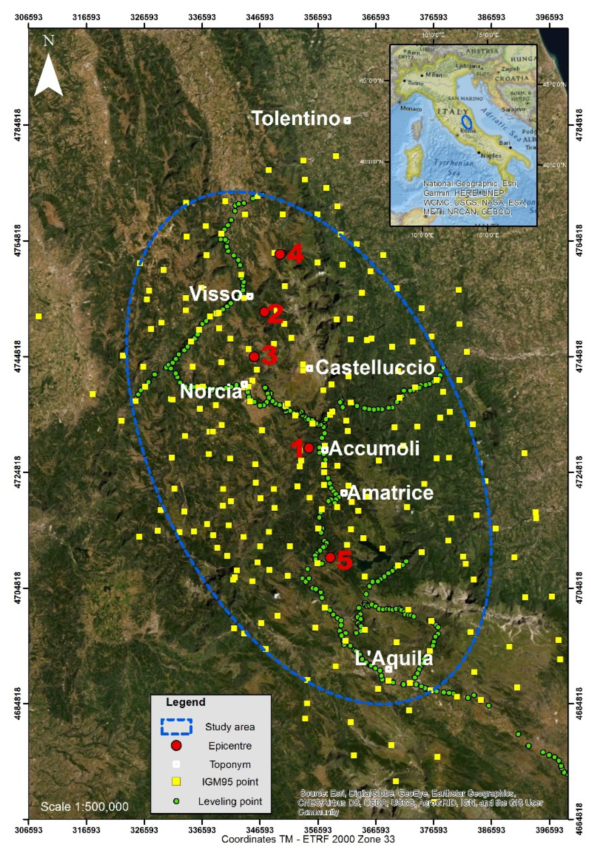
To identify the area affected by the major movements, two summary reports published by the INGV after interferometric analyses of the seismic events were utilized [
57,
58]. The area affected by the major movements extends from northwest to southeast, i.e., from Tolentino (Province of Macerata, Marche Region) to L’Aquila (Abruzzo Region). The area where GNSS surveys and geometric leveling were carried out is highlighted by the dashed line in
Figure 3, which shows the position of the five considered earthquakes (the same as
Table 1) and the IGM95 network points.
3.1. GNSS Data Surveying and Processing
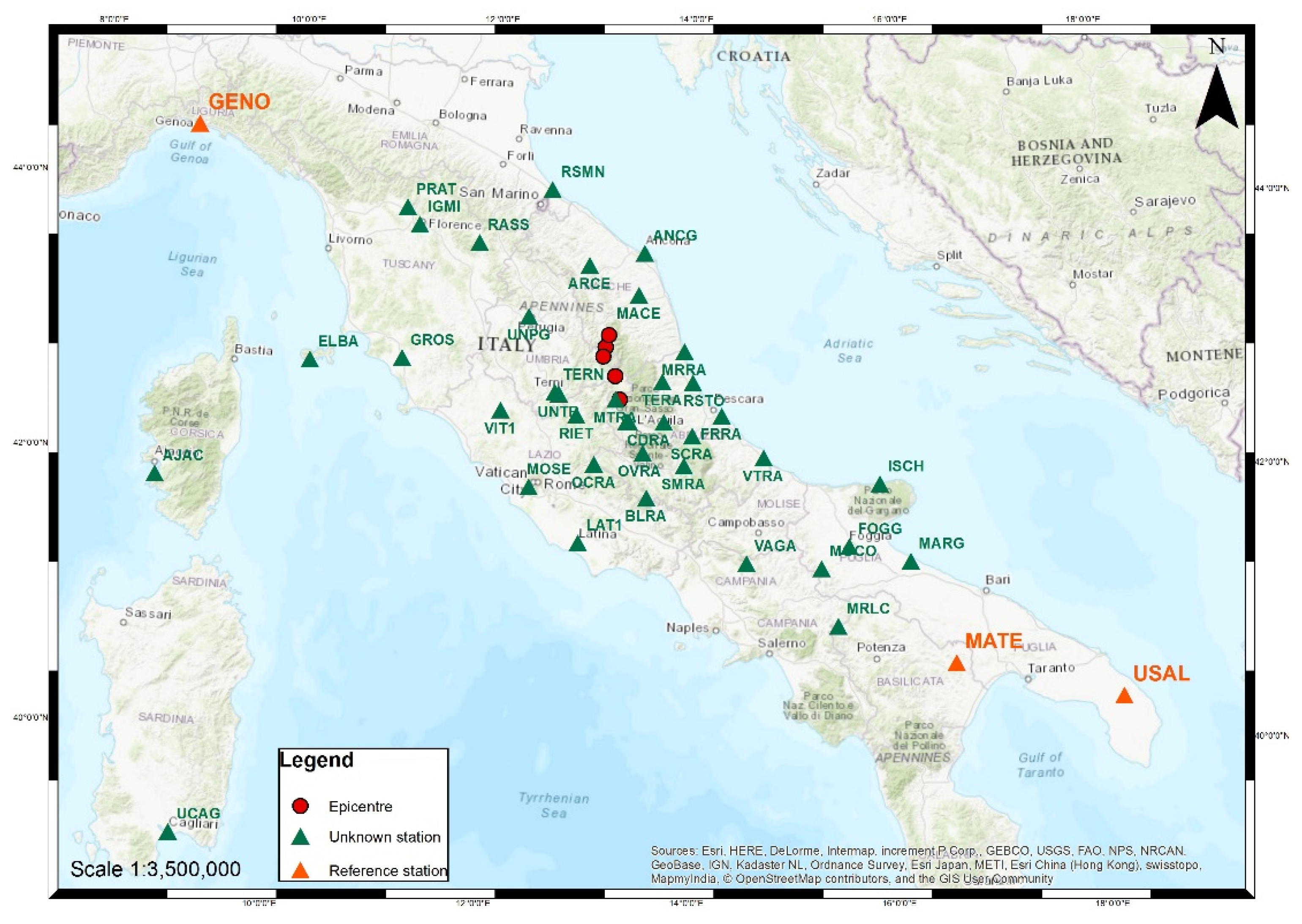
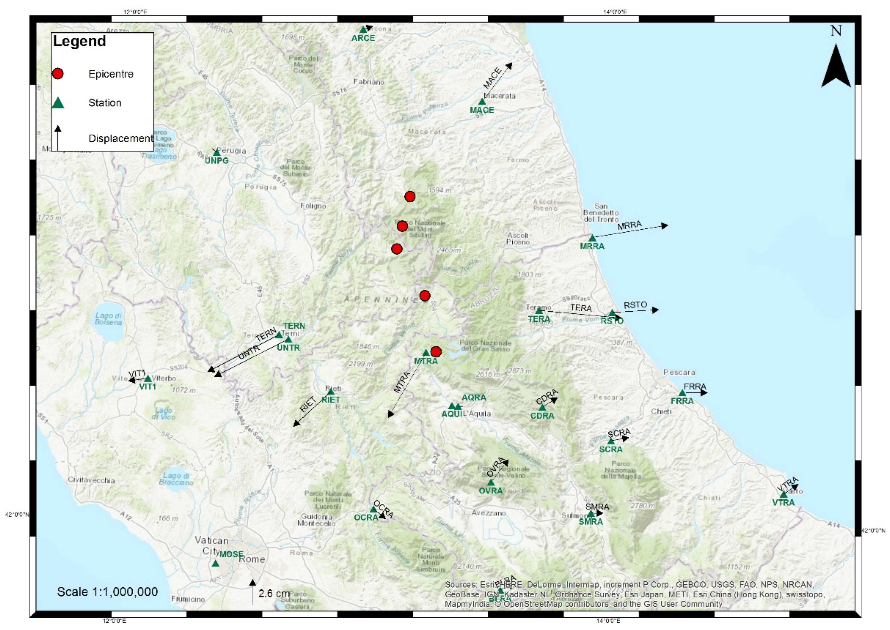
One of the first decisions to be taken was identifying the stable points to be used as a reference for displacement calculations. Since the real extent of the area affected by the earthquake was only partially known, it was necessary to undertake topographic surveys outside the area affected by the most evident damages to highlight the effective movements. While trying to reduce the effort and limit the size of the area, it was analyzed the behavior of the permanent GNSS stations present in the area, thus taking advantage of already available data. In particular, the following 21 GNSS permanent stations of the national RDN (Rete Dinamica Nazionale—National Dynamic Network) and regional networks (Abruzzo, Marche, Umbria and Lazio regions) were used: AQRA, AQUI, ARCE, BLRA, CDRA, FRRA, MACE, MRRA, MTRA, OCRA, OVRA, RIET, RSTO, SCRA, SMRA, TERA, TERN, UNPG, UNTR, VIT1, VTRA. To include stable points in the network that are outside of the area affected by the movements, 33 additional GNSS stations were added to the database—most of them are in Central Italy, but others included to obtain a correct georeferencing are located at a great distance (up to 900 km). Therefore, in total, 54 GNSS permanent stations were used in this study.
The calculation of the GNSS permanent station coordinates was carried out by using the Bernese GNSS Software (5.2 version). The software, developed at the Astronomical Institute of the University of Bern (AIUB) by a team of researchers [
59], is a scientific code characterized by the highest quality standards for geodetic analyses further applications based on GNSS data. Within Bernese, the GNSS observations available in daily RINEX file format, acquired in 6 or more consecutive weeks, were processed. Data refers to two distinct periods: before and after the seismic events. The first period is represented by 49 daily sessions between the 1904 and 1910 GPS weeks corresponding to the period from 3 July to 20 August 2016; the second period is related to 42 daily sessions between the 1933 and 1938 GPS weeks corresponding to the time span 22 January–4 March 2017. Both calculations, performed by the same workflow described hereunder in the text, were referred to the IGb08 global system according to strategies suggested by the EUREF guidelines (
http://www.epncb.oma.be/ accessed on 9 February 2022) in force at the time of the processing (summer 2017). The following stations were chosen as a reference because, even if quite far from the earthquake areas, they belong to the A class of the European EPN network, characterized by position and speed, with an accuracy lower than 1 cm and 1 mm/year respectively: BZRG, COMO, EBRE, GENO, GRAS, GRAZ, MATE, NOT1, USAL, WTZR, ZIMM, SOFI.
Figure 4 shows the position of some reference stations and that of stations to be calculated.
The data processing was carried out using the precise ephemerides made available by the International GNSS Service (IGS) and the calibration file of the IGb08.atx antennas.
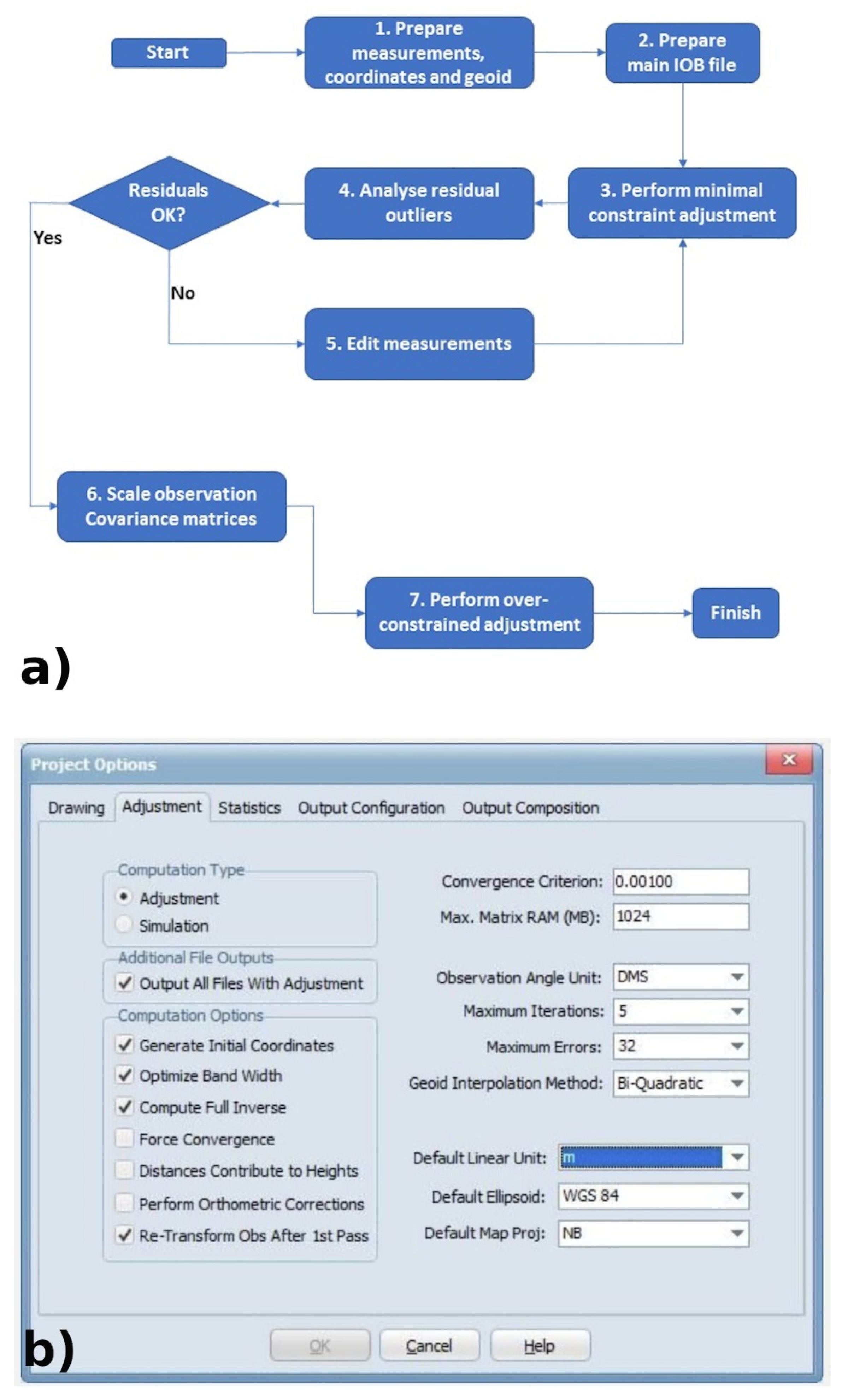
The determination of the station positions in both periods was divided into two phases: the first phase concerned with the calculation of the network’s daily solutions expressed as normal equations relating to the above observation sessions. For this type of processing, the standard procedures developed by AIUB were followed. In the second phase, performed using the ADDNEQ2 module of the Bernese software, the network was adjusted on the basis of the reference stations positions; the procedure was carried out according to the minimum constraints’ method (three translations) by combining the normal equations as computed in the previous step. Thus, the final coordinates of the stations were obtained and expressed in the IGb08 system and temporally referred to as the central moment of each period: 27 July 2016 (epoch 2016.6) for the period before the main earthquake and 11 February 2017 (epoch 2017.1) for the period after the mainshocks.
To determine the displacements caused by the earthquakes by comparison of the station positions in the two periods, it was necessary to exclude the translations related to the tectonic plate movement (approximately 3 mm/year). The removal of this component was done by transforming the coordinates referred to the IGb08 into the ETRF2000 system, which is based on the Eurasian plate. Italy has adopted as an official reference (Decree of the Council of Ministers Presidency dated 10 November 2011) the implementation of the European system ETRS89, named ETRF2000 at the time, called 2008.0. The IGM has materialized this system in Italy by assigning the coordinates to the RDN network and, with a little less precision, to the IGM95. The materialized points of these networks, distributed throughout the national territory, represent the system. The GNSS is a relative determiner; thus, it determines the vectors in space (baseline) with high precision that connect the unknown points to the aforementioned networks; the determination of the new points in the official national system is thus obtained.
The method suggested by EUREF for this transformation consists of applying seven roto-translation parameters updated to the moment of interest, using the coefficients published by Boucher and Altamini [
60]. In this work, the coefficients published by EUREF and related to the periods of interest (i.e., 2016.6 and 2017.1) are shown in
Table 2.
By applying these parameters to the results expressed in the IGb08 global system, the coordinates of the stations in the ETRF2000 system were obtained for the two periods (i.e., before and after the main earthquakes). Their spatial comparison represented the starting point for the evaluation of the displacements connected to the seismic events.
After obtaining a reliable permanent GNSS stations network characterized by known pre- and post-earthquake positions, a more detailed investigation of the area affected by the earth shocks was carried out. By measuring 452 baselines through static GNSS methodology, with stationing times always exceeding 2 h, a network of 250 points was generated, including 16 permanent local stations and 230 points of the IGM95 network that were essentially measured in 1992 and refined in 2001; the remaining part of the points belongs to the Lazio Region network, recalculated by IGM in 2006, but still not included into the IGM95 network. The position of many points of the IGM95 network is shown later in the text when the results are presented.
Five permanent local stations, namely AQRA, MRRA, MTRA, OVRA and TERA (
Figure 4), have a known position in view of the fact that they belong to the network already calculated by the Bernese software as previously described. By fixing their coordinates in a least-squares compensation calculation, performed within the GEOLAB software (Bitwise Ideas Inc.) as shown in
Figure 5, the post-earthquake position of the other 11 permanent stations was obtained.
Thirteen of the 16 known GNSS stations (i.e., AQRA, ASCO, AVZZ, CAMR, CSCA, FOL1, MRRA, MTRA, NRC2, OVRA, RIETI, ROIO and TERA), were chosen for their reliability and homogeneous distribution over the territory, were employed referentially in the GEOLAB software for a subsequent adjustment. This design provided the position of the entire network (250 points) with a mean square error of 9 mm. Although determined with high reliability, it must be mentioned that the ASCC, GINE and VCRA GNSS stations were not employed since they are considered not fundamental for the spatial distribution, and they showed a mean square error slightly higher than others.
Once more, the multitemporal comparison between the coordinates of 230 points of the IGM95 network (four of them have not been used for comparison because they are very close to other points and therefore considered not significant) allowed us to estimate the surface displacements in relation to the seismic events.
The maps of displacement were created in a Geographic Information System (GIS) by using the Inverse Distance Weighting (IDW) spatial interpolation method based on the points of known coordinates.
3.2. High Precision Geometric Leveling
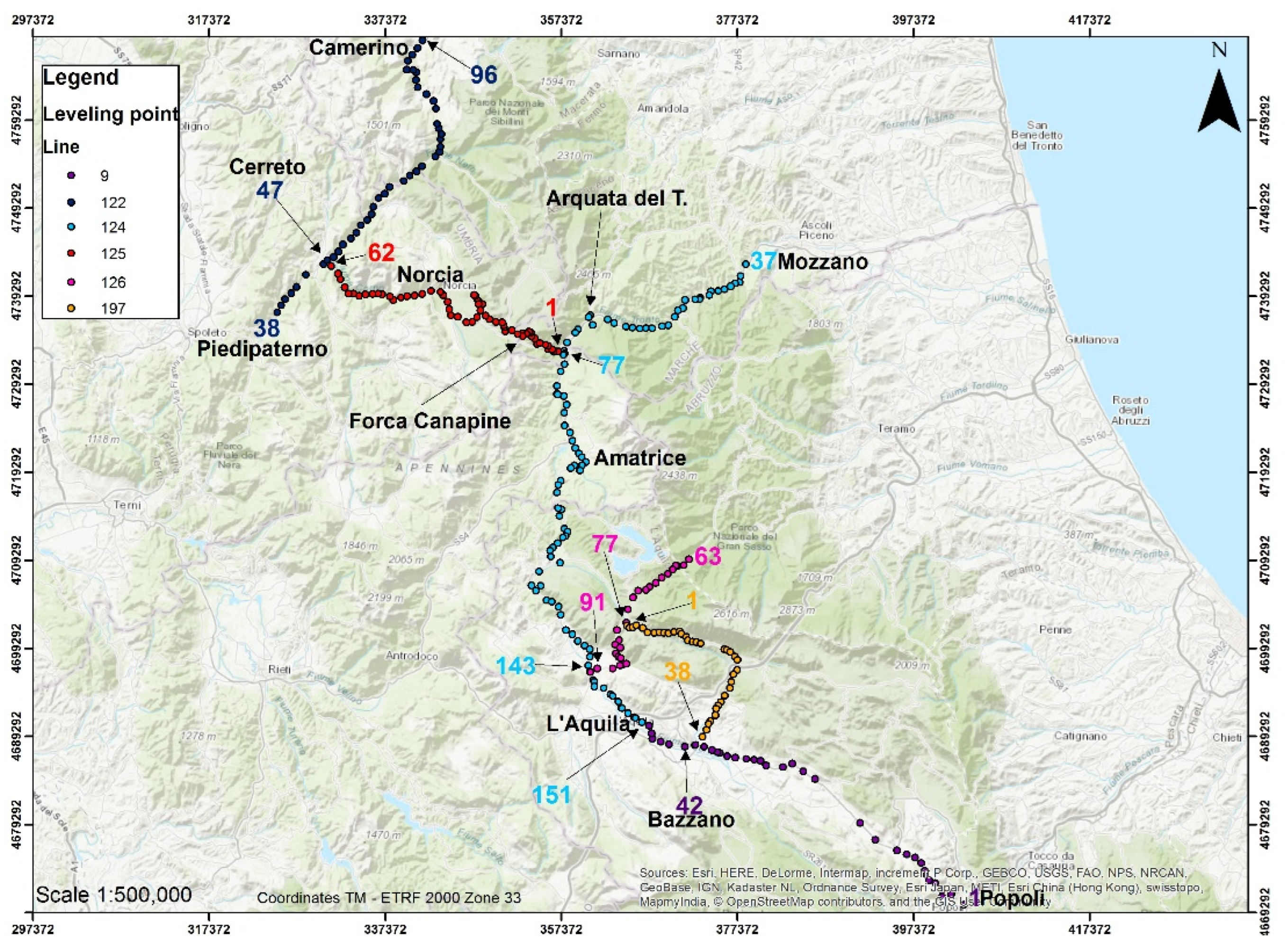
The study area is also characterized by the presence of geometric leveling lines that belong to the high precision national network set up by IGM in the early 2000s. All the lines falling within the study area were remeasured (
Figure 6) for a total length of about 350 km with an equivalent number of benchmarks. Theoretically, this allowed an additional estimation of the vertical movements connected to the seismic events and the improvement of the altimetric accuracy from the GNSS surveys. To have an external connection with benchmarks not affected by the seismic events, in the southern part, the remeasurement of line number 9 (
Figure 6) continued outside the area of interest until reaching the nodal point of Popoli. In particular, the following lines have been measured during the years 2017–2018:
Part of line number 122: from Piedipaterno to Camerino, for a total length of about 58 km.
Part of line number 124: from L’Aquila to Mozzano, for a total length of about 115 km.
Line number 125: from Pescara del Tronto to Cerreto, for a total length of about 60 km.
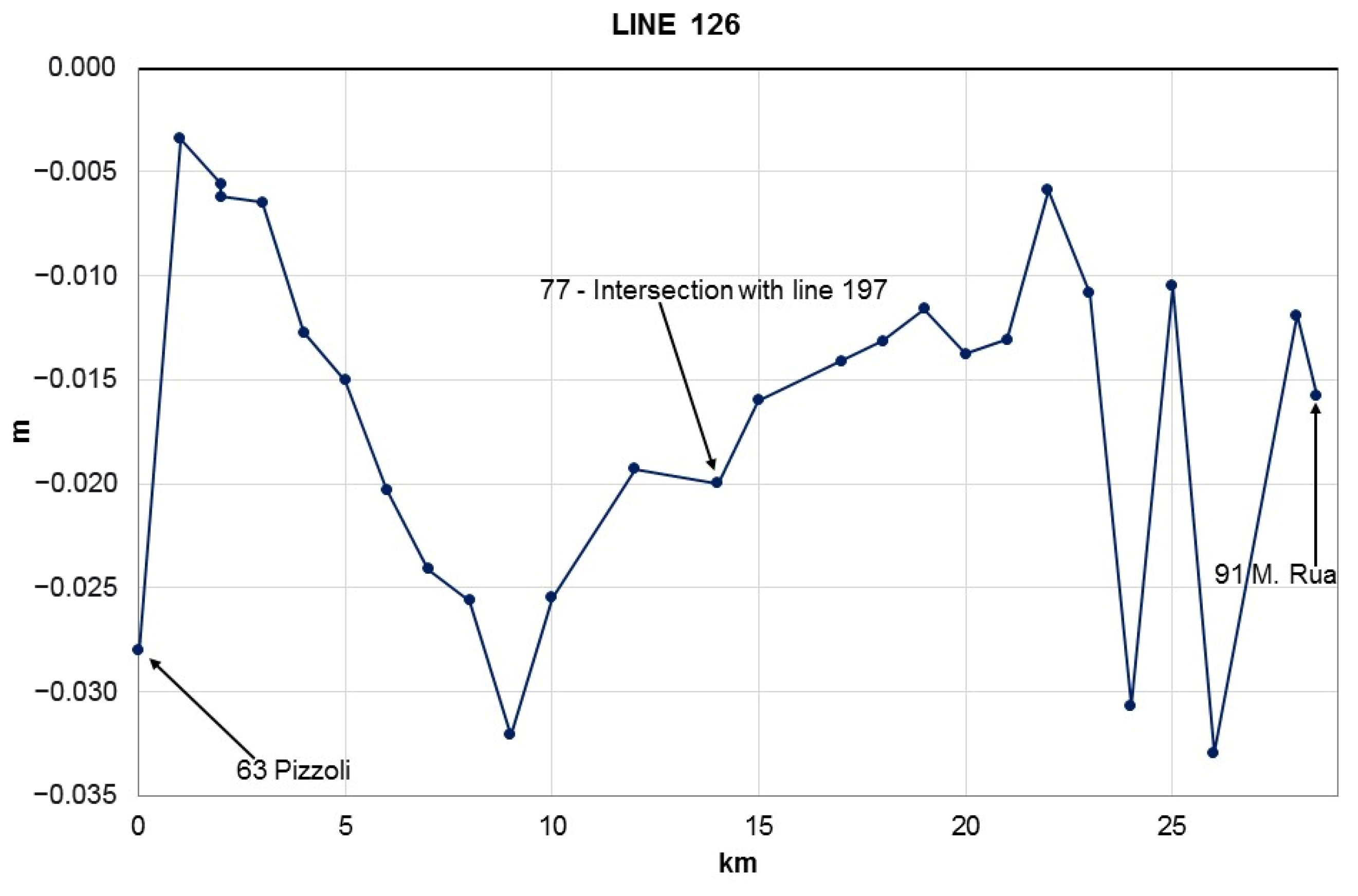
Part of line number 126: from Pizzoli to Monte Rua, for a total length of about 28 km.
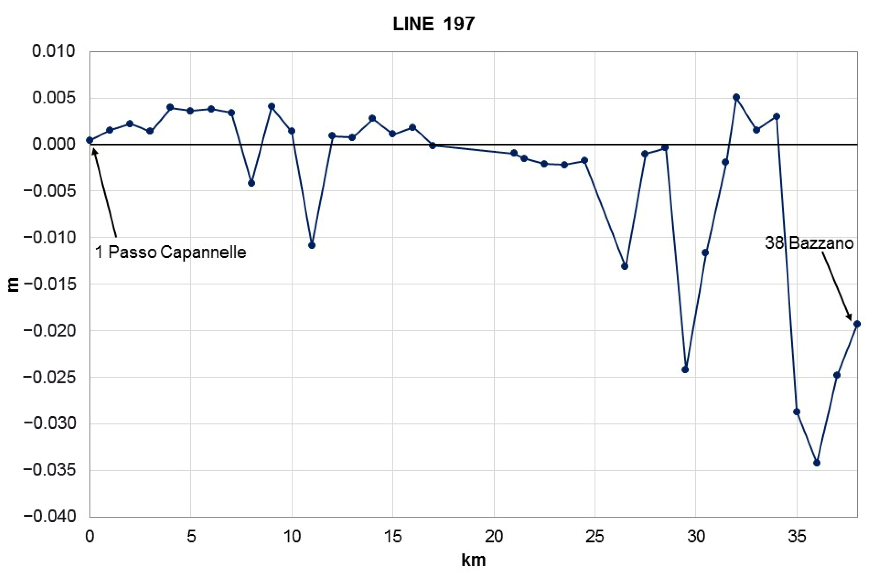
Line number 197: from Passo Capannelle to Bazzano, for a total length of about 38 km.
Part of line number 9: from L’Aquila to Popoli, for a total length of about 50 km.
Lines 122, 124 and 125 were initially measured in 2001, while lines 9, 126 and 197 in 2009. Among the total 350 remeasured benchmarks, only 300 maintained the original structure and allowed for a proper leveling and a correct subsequent estimation of the vertical displacement.
4. Results
The coordinates of 21 permanent GNSS stations present in the area of interest and in the surrounding zones and their differences as computed after the seismic events are presented in
Table 3. The GNSS stations with differences greater than 2 cm are highlighted in bold, considering this value as a threshold below which a possible uncertainty between real displacements and calculation errors is present. The data in
Table 3 shows how coordinate differences of GNSS stations before and after the earthquake are quite small, probably due to the considerable distance of the sites from the earthquake epicenters.
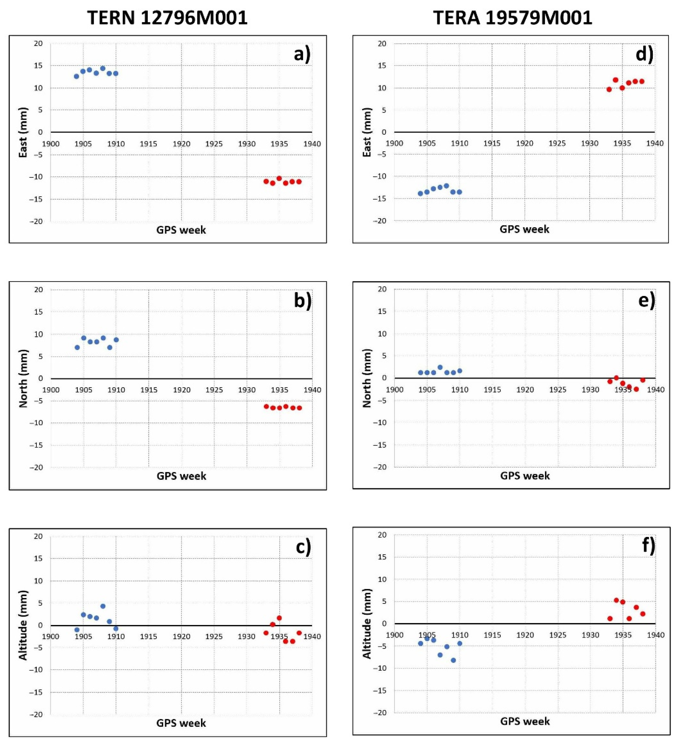
Figure 7, for instance, shows the trends of the coordinates of the Terni (TERN 12796M001) and Teramo (TERA 19579M001) GNSS stations that have experienced maximum planimetric displacements of approximately 26 mm. Belsorano GNSS station (BLRA 19567M001) is characterized instead by the maximum altimetric displacement (i.e., 116 mm,
Table 3).
Figure 8 shows the planimetric displacements of all the stations located in the area affected by the earthquake and in the surrounding zones.
The accuracy of GNSS surveying must respect the IGM guidelines. The IGM has never published official technical specifications since there is no experience of more than a century on GNSS differently than the geometric leveling described below. Nevertheless, updated technical specifications were used because of technological innovations that rapidly followed. Since the error analysis on points with 2 h of stationing largely depends on the local conditions (e.g., number of visible satellites, their spatial arrangement, the presence of obstacles and of cycle slips, etc.), to assess the quality of the executed measurements it was referred to [
61,
62]. One hour of the static surveying method between the bases with a distance less than 10 km from one to the other results in an expected accuracy of 1.5 cm [
61] and 1.0 cm (from 10
−6 to 10
−8 ppm [
62]).
By setting the international stations with coordinates estimated by the EUREF, the 13 permanent stations closest to the area of interest were calculated by using Bernese GNSS Software and an error lower than 1 cm was obtained. Then, the adoption of a stationing time never shorter than 2 h allowed for the measurements of 452 bases that connect 250 points, including the 13 permanent stations already calculated. The average length of the bases was about 9 km. The adjustment performed by GeoLab Software provided the following results expressed at a 95% confidence level: (i) the RMSE of the weight unit is 5 mm (in the text, we previously wrote 9 mm because, in our opinion, it was conducted with the most reliable repeatability); (ii) the mean value of the major semi-axes of the planimetric absolute error ellipses is 16 mm; (iii) the average value of the absolute altimetric errors is 81 mm (for this reason, we used the leveling heights instead of those from the GNSS survey); (iv) the mean value of the semi-major axes of the relative planimetric error ellipses (i.e., errors on the bases) is 15 mm; (v) the average value of relative altimetric errors is 12 mm.
Finally, the error analysis executed for the 2 h observations of the GNSS surveying was considered acceptable because it was obtained from a significant amount of data, and it supported the reference theory [
61,
62]: 2 h with bases at 10 km that result in an accuracy lower than 15 mm.
In terms of the high precision geometric leveling, the analysis of altitude differences of each line shown in
Figure 6 allowed us to estimate the vertical displacements connected to the seismic sequence. The accuracy of these estimations follows the technical specifications published by the IGM [
63], where the fundamentals for the execution of high-precision geometric leveling are described. These are some of the most significant guidelines:
- −
A leveling instrument, positioned between a backsight and a foresight rod for measuring fractionated sections, must be used;
- −
The distance between the leveling instrument and the rod must not exceed 40 m and, consequently, the length of a section must not exceed 80 m;
- −
The height difference of each section must be measured twice (foresight and backsight) in a totally independent way;
- −
The discrepancy between the foresight and backsight height difference of each section must not exceed the following tolerance:
where L is the length of the entire vertical control network expressed in kilometers;
- −
When the tolerance is respected, the average of the foresight and backsight values is assumed as the difference in the height of each section.
In the case of the post-seismic measurement, entire lines were not remeasured between nodal benchmarks, but only partial sections where preliminary investigations led to suspect possible displacements. In any case, the measurements were continued until five consecutive differences in height were found both at the beginning and at the end of the line in tolerance with the previous data. As a further check, it was always verified that the remeasured vertical control network was in tolerance with respect to the benchmarks remaining fixed at the beginning and the end, with a difference between the new and previous differences in height lower than:
Given the substantial experience of the IGM’s personnel, it is notorious that the high precision leveling implemented with these technical specifications allows for the precision in height differences of 1 mm per km.
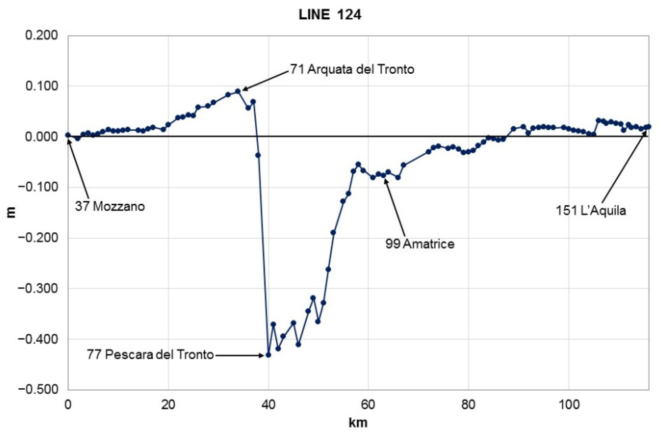
For line number 124 (
Figure 9), the new measurement started from the locality of Mozzano, where, for the first 20 km, no significant variations were noted. The next 14 km showed gradual increases up to a maximum of +9 cm in Arquata del Tronto (
Figure 6) which was dramatically experienced by the mainshocks; a sudden drop followed which, in approximately 6 km, seemed to exceed −40 cm in Pescara del Tronto. From here, a recovery of the lowering—first rapid and then slower—continued for about 50 km until the locality of Montereale, which appeared to be stable. The last 25 km, up to the city of L’Aquila, did not show significant altimetric differences.
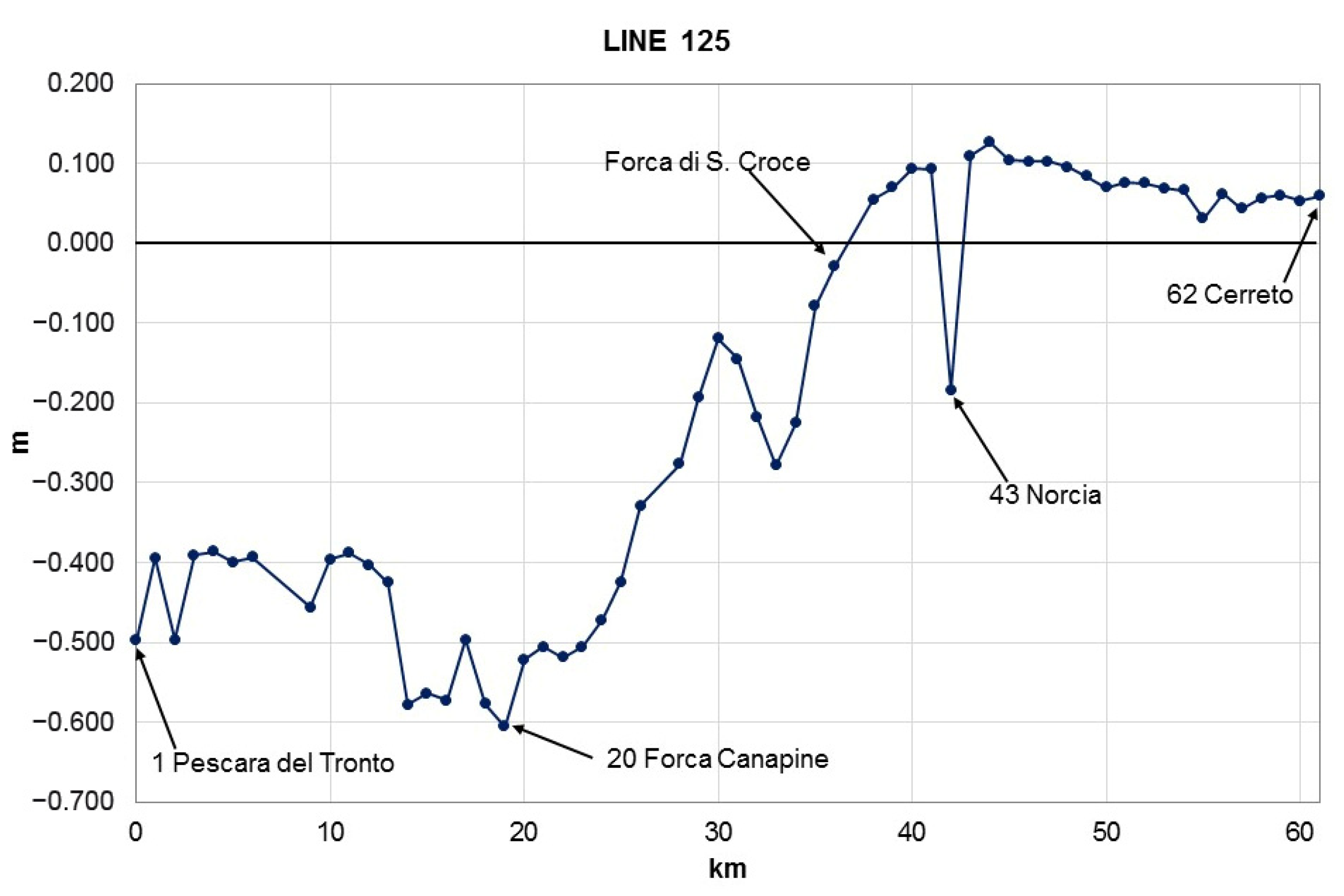
Line number 125 (
Figure 10) is hooked up to the benchmark of number 77 of line 124 in Pescara del Tronto where the already-reported significant drop (
Figure 9) showed an increase up to −50 cm. In the first 20 km, the lowering increases further, up to a maximum of −60 cm in the area of Forca Canapine. From here, the decrease of the lowering starts and continues for about 15 km up to Forca di Santa Croce where parity is reached. The next 8 km, excluding the anomalous benchmark of Norcia, showed an uplift of a maximum of +12 cm. In the last 18 km of the line, the rise gradually decreases up to 6 cm in the locality of Cerreto.
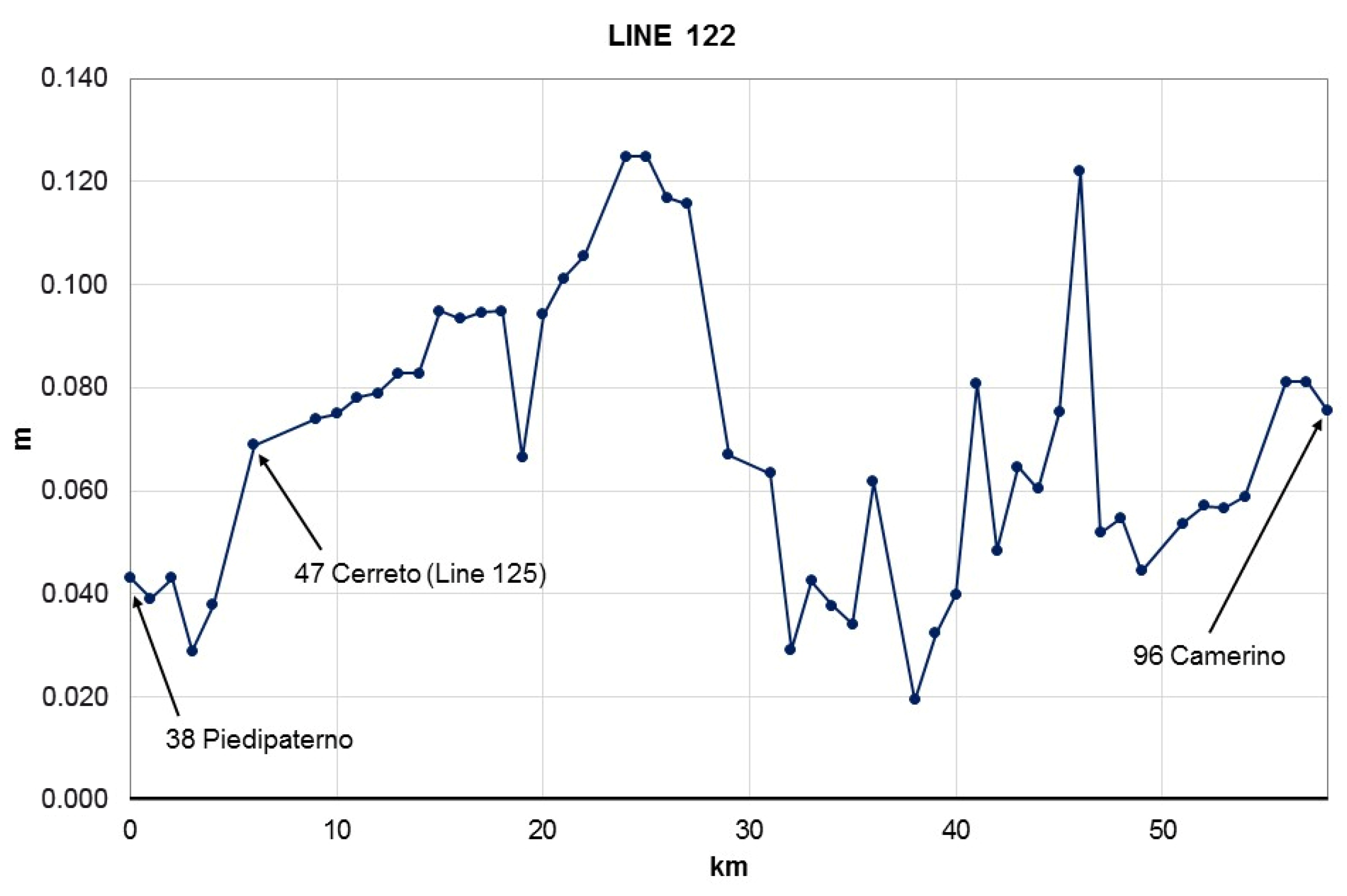
Line number 122 (
Figure 11) was remeasured starting from the connection with line number 125; the uplift of 7 cm measured in Cerreto slightly decreases towards the southwest up to 4 cm in Piedipaterno and increases towards the northeast for about 18 km, reaching the value of +13 cm. Then, the trend decreases for the following 13 km until a lower value of +2 cm. The last 22 km are characterized by fluctuating values of the rise ending with +7 cm of uplift in the city of Camerino.
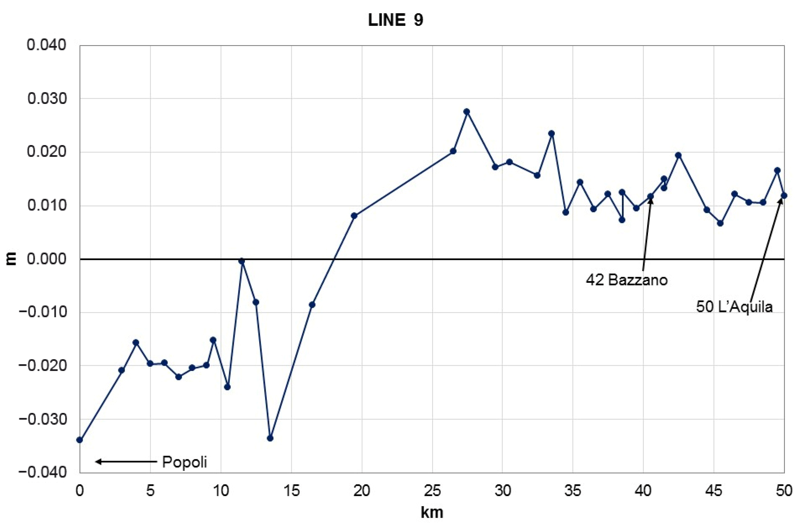
Line number 9, whose profile of altitude differences is shown in
Figure 12, is within the area of the earthquake 20 km northwest of Popoli with a low rising value of about 1 cm. In the following part, the altitude differences wave for the 30 km were around very low positive values; in the localities of Bazzano and L’Aquila, where lines number 197 and 124 begin, respectively, line number 9 reports uplift values of +1.5 and +1.2 cm, respectively.
In the southern part of the study area, altitude differences resulting from the geometric leveling of lines number 126 (
Figure 13) and number 197 (
Figure 14) indicate small-scale movements waving around the values of +0.5 and −3.5 cm.
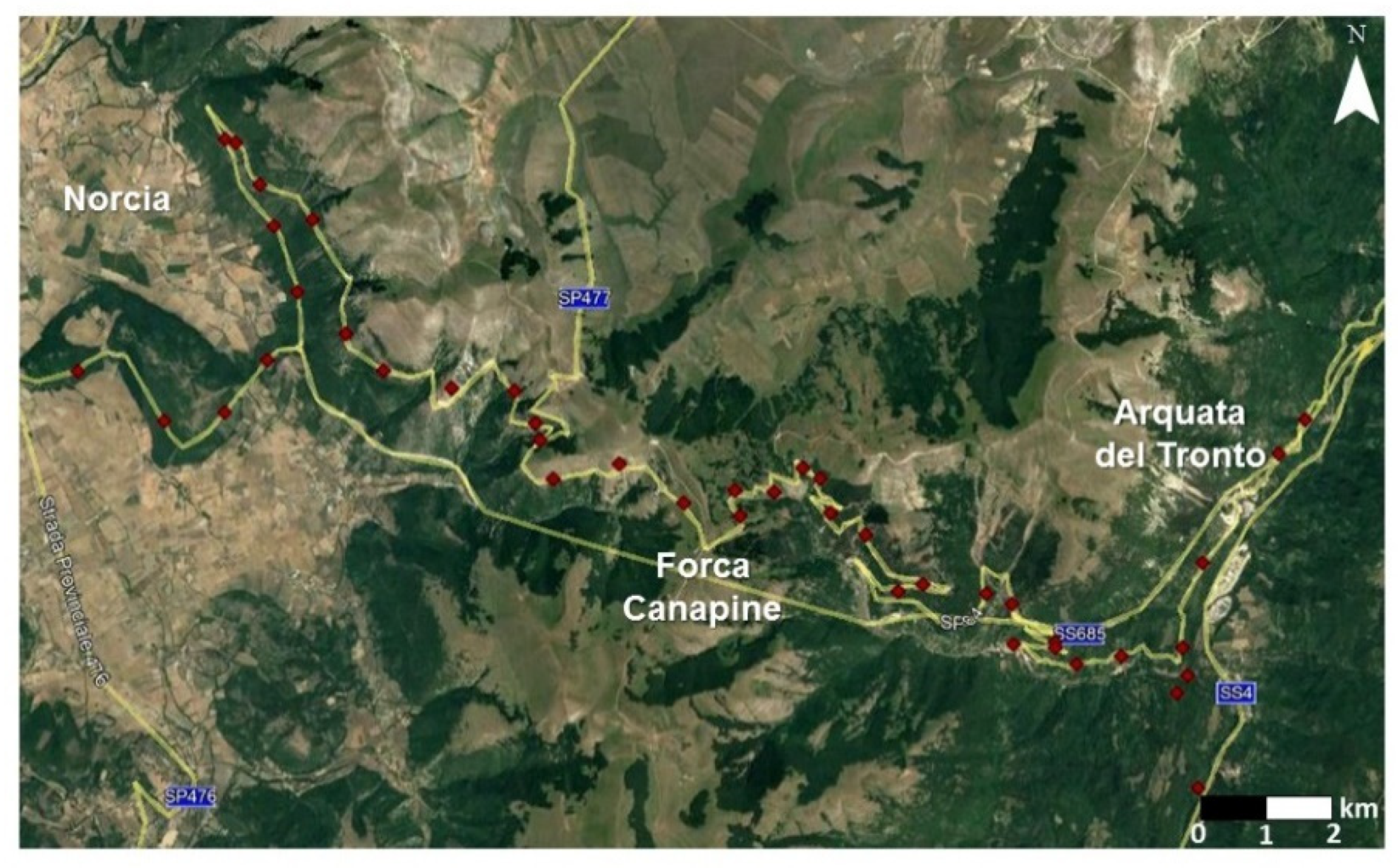
In some cases, the analyzed profiles have trends that are difficult to interpret with standard deformation models since they show sudden alternations of decreases and rises with values reaching up to 20 cm. This fact can be partially related to the presence of a series of hairpin bends (
Figure 15) that distort the calculation of benchmarks position. In the resulting profile, the benchmarks are spaced between many kilometers despite being planimetrically very close.
Both of the obtained results, one from the processing of GNSS data and the other from geometric leveling, allowed for the comparison between the pre- and post-earthquake positions of the analyzed benchmarks as well as the estimation of the relative ground displacements. In particular, the multitemporal comparison between the coordinates of 230 points of the IGM95 network allowed the estimation of movements in relation to the 2016–2017 seismic sequence.
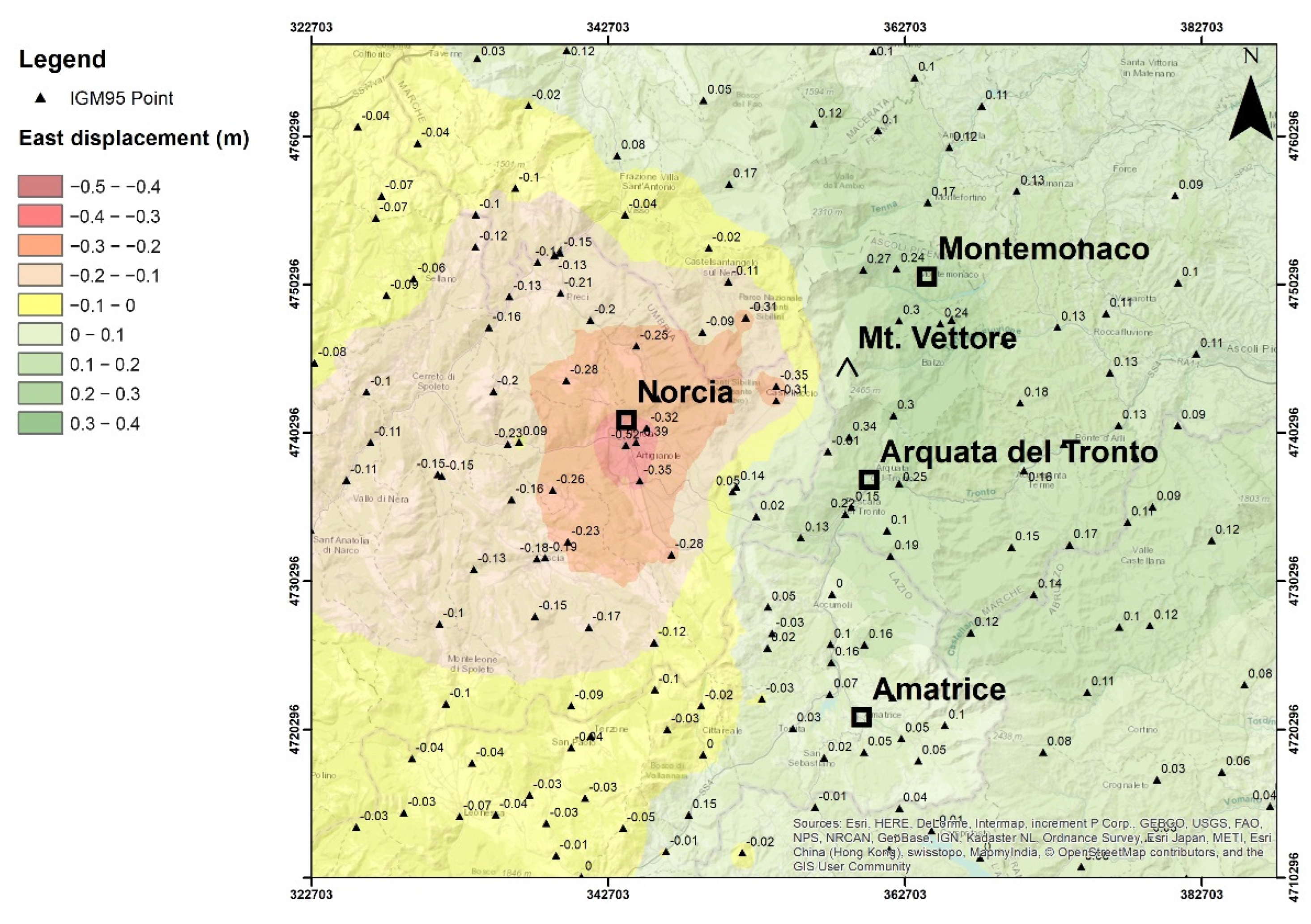
The analysis of the planimetric differences highlights both negative and positive trends; the maximum decrease of the east coordinate (equal to −52 cm), which corresponds to a westward movement of the ground, is recorded in the locality of Norcia (
Figure 16).
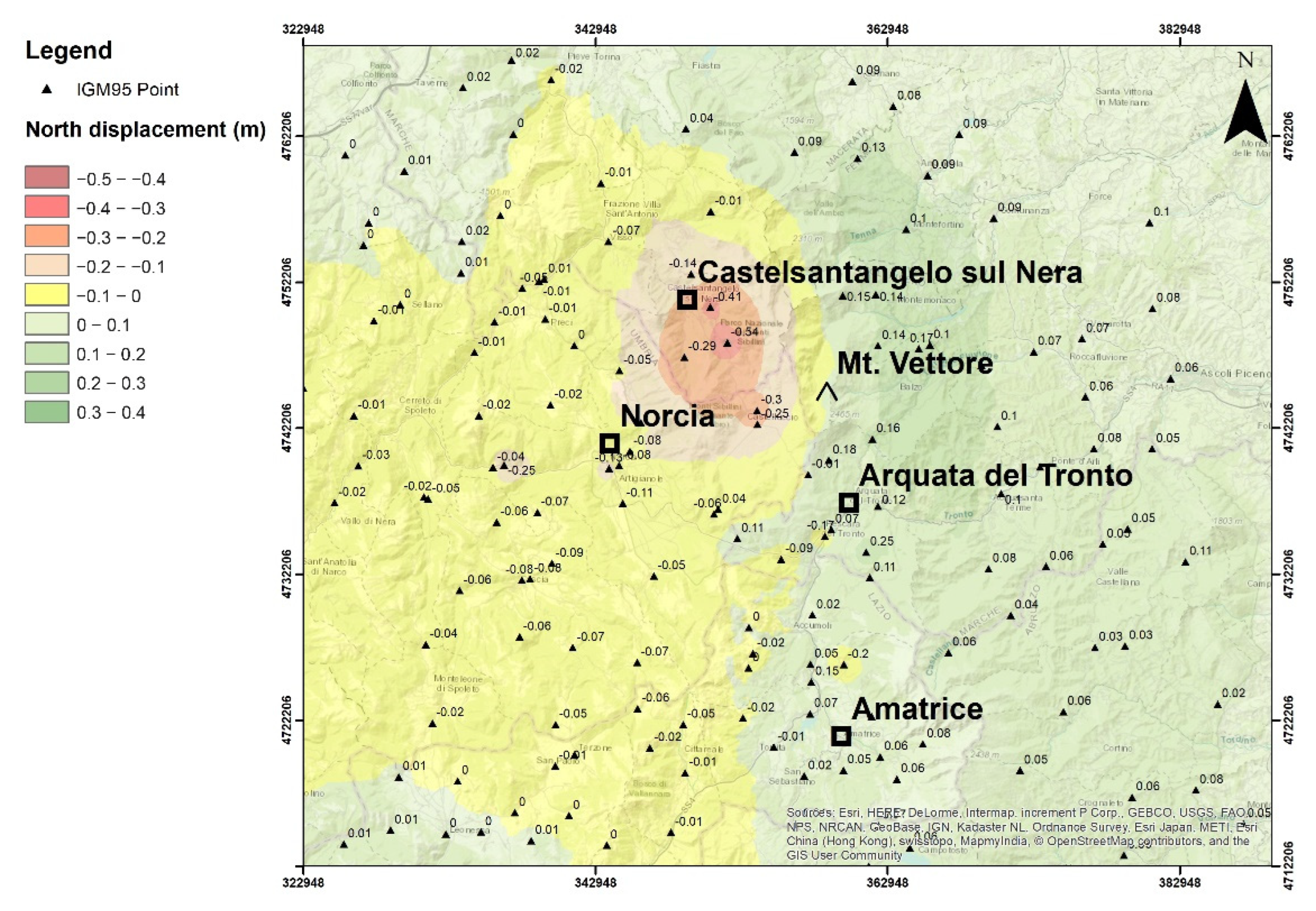
From this location, moving eastward, smaller shifts have been highlighted until the east coordinates show positive increases reaching their maximum in the locality of Montemonaco (+27 cm). This trend is confirmed by the analysis of changes in the north coordinates, which are spatialized in
Figure 17: the boundary between positive and negative values is very similar to that of
Figure 16. While the maximum southward displacement (decrease of the north coordinate), equal to −54 cm, occurred in the north of Castelluccio (between Norcia and Arquata del Tronto, immediately west of Mt. Vettore), the maximum northward movement (increase of the north coordinate) of +25 cm was registered immediately south of Arquata del Tronto.
5. Discussion
The results from this analysis have been compared with several studies on the same area published in recent years. In planimetry, the obtained maps (
Figure 16 and
Figure 17) show in the area of Norcia a clear westward movement with a maximum amplitude of about 50 cm, in agreement with Cheloni et al. [
21]. The authors also highlighted a slight uplift of about 15 cm in the surroundings of Norcia, similar to our results with a maximum local rate of 12 cm. Moreover, Cheloni et al. [
21] described an eastward displacement of the footwall of VBFS, east of the Vettore Mount, with a maximum amplitude of about 30 cm. The GNSS site named VETT, described in Xu et al. [
23], shows the maximum horizontal displacement of 36 cm and 13 cm for the east and north components, respectively; in the same area, we found eastward and northward displacements with a maximum amplitude of about 30 cm and about 15 cm, respectively. Still, in agreement with our results, Wilkinson et al. [
26] compared their measurements, obtained by one short-baseline GNSS dataset for the Norcia earthquake, with Regional GNSS stations [
58] and present horizontal coseismic displacements of 38.3 cm north–east (GNSS station VETT, in the footwall of VBFS) and 26 cm south–west (GNSS station MSAN, hanging wall). Pousse-Beltran et al. [
27] in the area between Norcia and Amatrice report on post-seismic surface displacements that reached 35.5 ± 1.7 mm in ascending Line Of Sight (LOS) of SAR scenes by January 2017 and reached 50.5 ± 2.1 mm on 30 April 2017; in the same area we have found post-seismic surface displacements varying from −3 cm to −60 cm. The LOS values in ascending data shown in Xu et al. [
23] document major motion towards the satellite ranging from −50.1 cm to 26.7 cm, in agreement with Bignami [
64], where deformations toward the satellite varied from about −50 cm to about 27 cm. One ALOS-2 interferogram in Xu et al.’s study [
23] spanned the Norcia earthquake and showed LOS values ranging from −66 cm to −22 cm. Wilkinson et al. [
26] measured the absolute vertical coseismic displacements of a 5.5 cm uplift (VETT, footwall—in the same area, we computed displacements up to 10 cm) and 44.6 cm of subsidence (ARQT, hanging wall—in the same area, we calculated displacements greater than −50 cm). Papadopoulos et al. [
32] found the maximum ground subsidence in the area of Norcia equal to −35 cm from the DInSAR analysis.
The analysis of the altimetric changes resulting from the geometric leveling highlights the presence of vertical movements of considerable entity, clearly higher than those observed during the main seismic events which had previously affected the national territory in the last decades (earthquakes of Umbria Region 1997, city of L’Aquila 2009, Emilia-Romagna Region 2012).
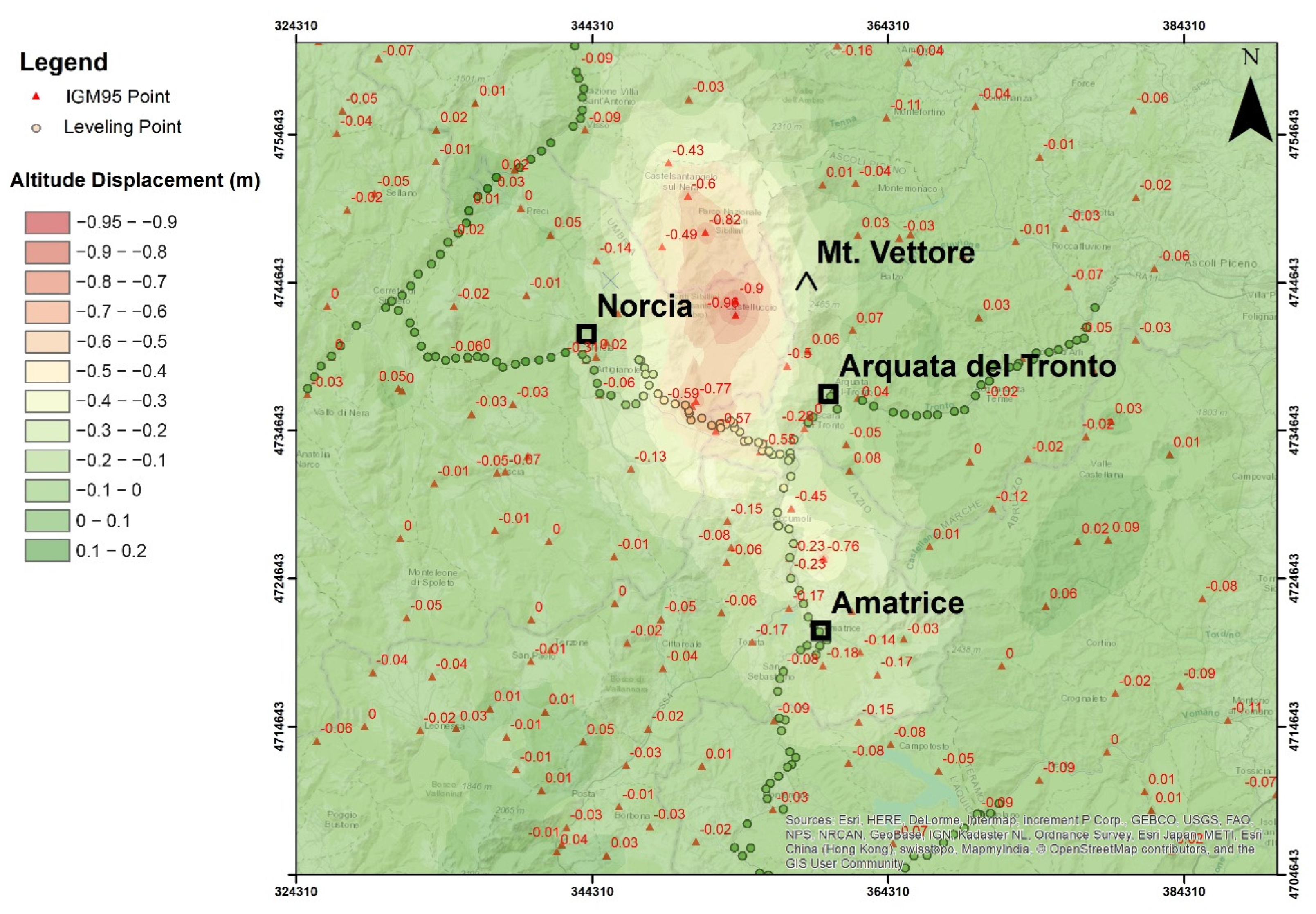
Figure 18 shows the altimetric differences as recorded in the 350 benchmarks before and after the seismic events. The differences obtained from the IGM95 network analysis are represented by triangles and labels, while the data related to the geometric leveling are reported through dots using the color scale of the map.
The comparison between the data obtained from the two methodologies indicates a satisfactory agreement in such a way as to validate their correctness. Somewhere, the non-perfect correspondences are due to the interpolation algorithm of the IGM95 network points and the subdivision of the results into classes of 10 cm; on the other hand, a more detailed subdivision would have worsened the graph’s readability by creating an excessive number of color shades. The altimetric displacements are almost totally negative, with a maximum lowering value east of Norcia at the locality of Castelluccio (−95 cm), on the west side of the Vettore Mount. Moving away from this site, the lowering decreases in all directions, and it ends at distances of about 15 km to the east and the west and 30 km to the south and north.
Moving toward the east in the area of Castelluccio, we obtained a westward movement with a maximum amplitude of about 35 cm, in agreement with data from Cheloni et al. [
21], where localized westward motions reach up to about 60 cm were described. A southern component is also present, with a maximum amplitude of about 50 cm north of Castelluccio, near Castelsantangelo sul Nera. However, the major displacements have been detected by analyzing the altitude data, with maximum subsidence of about 1 m in the proximity of Castelluccio and other high values in the whole area between Norcia and Accumoli with lower rates up to Amatrice. Cheloni et al. [
21] showed the maximum detected subsidence of about 90 cm in the surroundings of Castelluccio. Pousse-Beltran et al. [
27], in the Castelluccio basin, presented lower LOS displacement values that attained 13.2 ± 1.4 mm in the ascending line of sight on 6 January 2017 and reached 37.9 ± 1.3 mm on 30 April 2017. Furthermore, Papadopoulos et al. [
32] presented the maximum ground subsidence in the area of Castelluccio as equal to −67 cm from DInSAR analysis and −22.5 cm east from Castelluccio (similar to our results, up to −25.5 cm in the hanging wall of VBFS). Our results also support those of Huang et al. [
28] in terms of the horizontal components in their work based on Sentinel-1’s decomposing ascending and descending interferograms.
To the south, in the area of Accumoli, InSAR results from Huang et al. [
28] show that most of the coseismic displacement is in the vertical direction; there are two main coseismic subsidence areas with peak vertical displacements of about −20 cm and −19 cm north and east of Accumoli. These results agree with our findings even if we have greater subsidence rates in the area (up to −40 cm) and the major values are localized west of Accumoli. A southern component of displacement is also present, with a maximum amplitude of about 18 cm between Accumoli e Amatrice.
Finally, in the zone of Amatrice and Campotosto, Cheloni et al. [
22] presented LOS subsidence with the maximum value of about 8 cm away from the satellite while, in the same area, we obtained values varying from −3 cm to −11 cm. Pousse-Beltran et al. [
27] documented ground surface movements away from the satellite by more than −6 cm in LOS in the area south of Amatrice affected by the Campotosto earthquake (18 January 2017). The maximum observed LOS change presented by Xu et al. [
23] in the Campotosto epicentral area reaches up to −9.6 cm for Sentinel-1 and −12.2 cm for ALOS-2.
From these comparisons, the obtained results agree with those existing in the literature, at least as far as the values of maximum cumulative deformation during the seismic sequence are concerned.
Furthermore, a short technical in-depth analysis is necessary: GNSS provides excellent results in terms of planimetry, while due to the technical nature of the system, the accuracy of vertical measurements was lower than the horizontal. In fact, satellites are orbiting (not geostationary) and constantly changing their arrangements. The receivers implement several algorithms to choose the best group of satellites for positional calculations (with a privilege for position rather than altitude). Furthermore, the Earth is not a sphere, and the mathematical model (ellipsoid and datum) contained in the receivers only partially compensates for the irregularities of the Earth’s surface. To complicate matters, it is also necessary to consider the fact that receivers are often unable to collect data from satellites below 10–15° of elevation because the signal must cross a very large thickness from the atmosphere and is too weakened and degraded. It is clear, therefore, that being able to “range” for 360° horizontally and only about 150° vertically, the vertical precision will always be less accurate than the horizontal one.
For this reason, we used GNSS in our work for the evaluation of planimetric deformations and mainly precision leveling for the evaluation of vertical deformations. Much of the works cited in the comparison between the values are also based on GNSS and many on DINSAR, which, if not treated with data in the ascending and descending orbits on permanent common scatterers, only allows for an evaluation of the deformation along the LOS, which depends on the angle of incidence of the satellite radar. Consequently, the assessment of the extent of the movement by analyzing the LOS alone must be treated with attention, to the point of considering it more from a qualitative perspective rather than from a quantitative one.
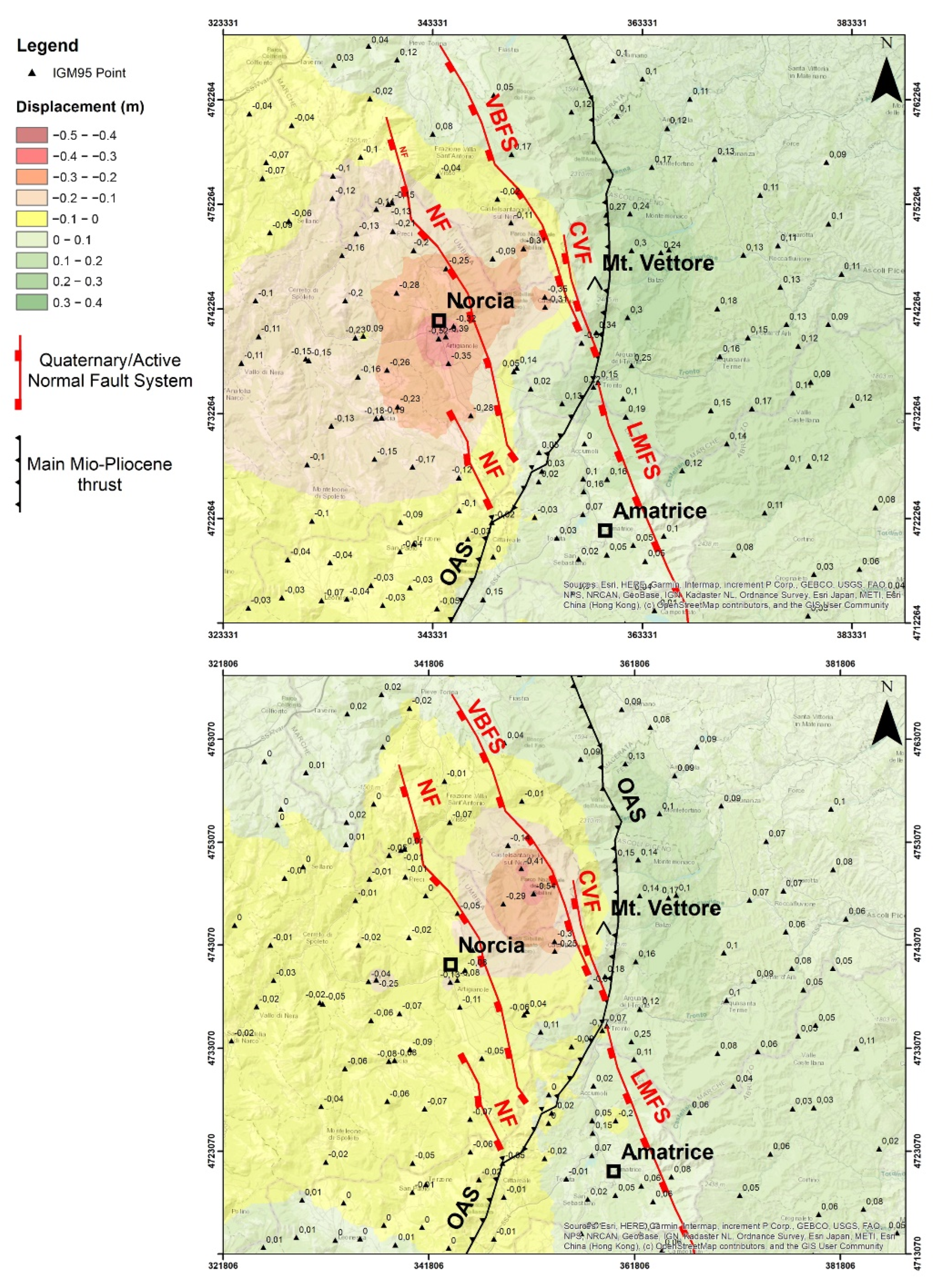
From the geological point of view, the results of our work are coherent with the regional tectonic setting of the area, which is dominated by the already mentioned VBFS and LMFS normal fault systems, trending northwest to southeast. This is clearly visible in
Figure 19 and
Figure 20, where draft representations of VBFMS and LMFS have been included in the displacement maps, and, in addition, the “Norcia Fault” (NF—[
65]) and the “Cordone del Vettore Fault” (CVF) have been included as well; the latter, considered active by Calamita et al. [
66], can be interpreted as an independent fault originated in the footwall of OAS [
3,
6].
The data from our study agree with other works that indicate the activation of the Mt. Vettore-Mt. Bove and Mt. Laga systems for the analyzed seismic event. Before the 2016–2017 seismic sequence, these systems were considered silent since no historical seismicity in this sector of the chain was documented [
6,
67]. On the contrary, the seismicity of the northern and southern sectors was already well known since they were recently struck respectively by the Colfiorito sequence in 1997 and the L’Aquila sequence in 2009. As previously indicated, Bonini et al. [
36], Cheloni et al. [
22], Falcucci et al. [
35], Improta et al. [
37], Pino et al. [
38], Porreca et al. [
31], Puliti et al. [
39] and Walters et al. [
30] documented how AOS acted as a geological barrier for the propagation of the rupture, delimiting the rupture of the first two seismic events (24 August 2016 and 26 October 2016) and subsequently acting as a stress concentrator probably leading to the third main event (30 October 2016) that crossed the barrier itself. VBFS and LMFS likely evolved separately during the Quaternary and started to kinematically interact in succession. Since the interaction may cause the formation of secondary structures [
68,
69], Pizzi et al. [
6] affirmed that in the study area, these structures were generated in the footwall of the OAS, creating a direct link between VBFS and LMFS, likely through CVF. The findings of these papers appear to be coherent with the topographic results of this study.
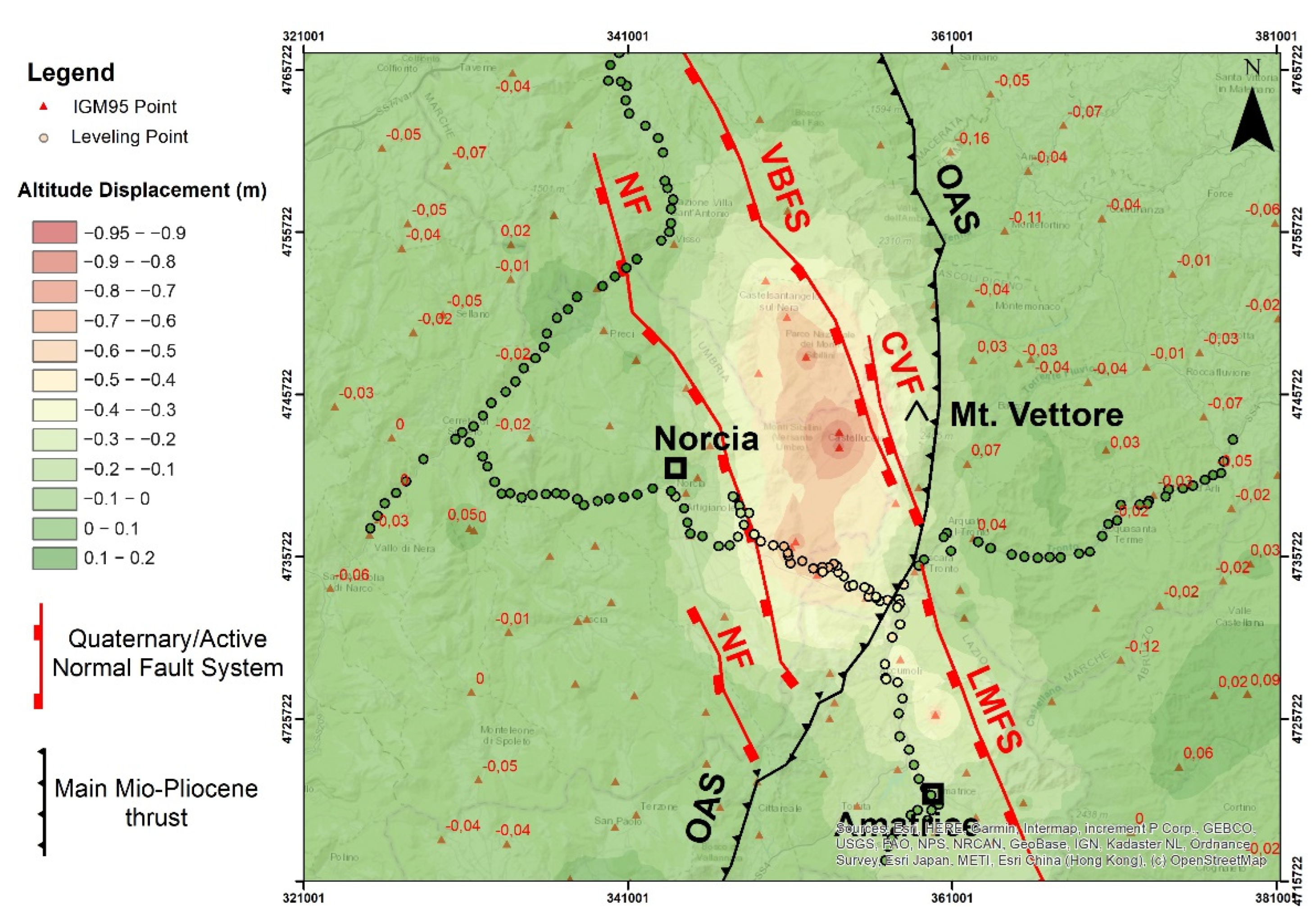
The eastward and westward displacements show an evident stop of their propagation in correspondence with the OAS thrust ramp. In addition, the altimetric differences are higher northwest and southeast of OAS, while they change in magnitude when crossing the thrust itself (
Figure 20).
Following this hypothesis, the OAS barrier in the future will probably be crossed, remaining as an irregularity on a unique continuous extensional fault system [
6].
Results from Cirella et al. [
24] confirmed a coseismic activation of the fault along the western flank of Mt. Vettore, as also suggested by Cheloni et al. [
21]. Analyses of these authors confirmed the previous findings, such as the prominent bilateral rupture, already documented by Huang et al., Lavecchia et al., and Tinti et al. [
28,
29,
70], with low to no-slip at the hypocenter and two well-separated slip patches. On the NW patch, the slip is maximum (nearly 1.3 m), and the rupture velocity is largely variable, between 2.2 and 3.2 km/s, in agreement with Liu et al. [
33]. Their study provides a complete description of the rupture propagation and inhibition due to the spatial distribution of rheological heterogeneities and the presence of inherited tectonic structures; the results corroborate the hypothesis that the rupture evolution of the 2016 Amatrice earthquake was strongly controlled by the presence of a tectonic structure, acting as a geometrical and rheological barrier; its location, trace, strike, and dip could be associated with the lateral ramp of the OAS. In addition, Porreca et al. [
31] provided a novel reconstruction of the subsurface geology of the area based on previously unpublished seismic reflection profiles and available geological data. They find that most of the seismicity is confined within the sedimentary sequence and does not penetrate the underlying basement (constrained at depths of 8 to 11 km). Their results allow us to better understand the rheological properties of the seismogenic rock volume, as well as the coseismic deformations of the topographic surface observed by geodetic techniques and field mapping.
Nevertheless, the bilateral rupture highlighted by strong motion and GNSS data does not provide conclusive information on the geometric configuration and earthquake-fault association. Lavecchia et al. [
29] have extensively explored multisensor/multiorbit DInSAR measurements to investigate the seismogenic source through analytical and numerical modelling techniques. The results revealed that the earthquake originated within the interlink zone at a depth between two seismogenic sources along two en-echelon faults connected at the hypocenter. Bonini et al. [
36] tested different tectonic models to conclude that the best fit between new data and previously published estimates includes partial or total reuse of inherited structures represented by steeper shallow faults overlying a master fault. The hypothesis is also supported by Falcucci et al. [
35], which affirm that OAS has played a major role in influencing the structural setting and evolution of the region, as well as VBFS has been re-used to accommodate the current extensional regime. Improta et al. [
37], presenting the first high-quality catalogue of early aftershocks of the three mainshocks of the 2016 sequence, document reactivation and kinematic inversion of OAS and its role in controlling segmentation of the normal faults. The spatial partitioning of aftershocks highlights that the OAS lateral ramp had a dual control on rupture propagation, behaving as a barrier for the Amatrice and Visso mainshocks and later as an asperity for the Norcia earthquake; they hypothesize that the Visso mainshock also re-activated the deep part of an optimally oriented pre-existing thrust. According to these authors, aftershock patterns reveal that the Amatrice aftershock and the Norcia mainshock ruptured two distinct antithetic faults 3–4 km apart.
Furthermore, Pavlides et al. [
34] confirmed the hypothesis that measured displacements are coherent with the regional tectonic setting of the area dominated by a fault and thrust system. They highlighted how the earthquake sequence from August to October 2016 had some special characteristics different from previous earthquakes either in the Apennines or elsewhere, such as widespread coseismic fractures and double events, quadruplicate seismic activity, and the fifth stronger event re-activating more or less the same fault segments. The surficial and, especially, the deeper geometry of the fault structures are very complex, following the thrust inherited structures that control the normal fault architecture, as well as the complex fault linkage and triggering of different fault segments.
Further evidence comes from the results of Walters et al. [
30]: they suggested that intersections between major and subsidiary faults controlled the extent and termination of rupture in each event in the sequence and that the structural barriers played a role in fluid diffusion, channeled along the fault intersections, and rupture re-initiation timing which lasted up to several months.
We can conclude that the understanding of the geological factors is very important to improve the possibility of predicting whether faults will fail in large, complex earthquakes or in temporally distributed seismic sequences of multiple large events. This knowledge and awareness represent important end-member scenarios with very different implications for seismic hazards.


