Review of Petroleum and Hydrogeology Equations for Characterizing the Pressure Front Diffusion during Pumping Tests

Abstract

In hydrogeology, the pressure front diffusion equation is crucial for the interpretation of pumping tests. It describes the displacement around the pumping well of the pressure front generated by a hydraulic disturbance, such as pumping or injection. This equation serves to physically locate the hydraulic objects (the recharge boundary, impermeable boundary, fault and hydraulic connection) that are able to influence the hydrodynamic behaviour of aquifers during a transient hydraulic test. However, several authors who have attempted to characterize this equation have come up with different expressions because the pressure front has been defined according to different approaches. This paper first clarifies the origin of the divergence between authors before reviewing seven approaches used to characterize the diffusion equation. In addition, a new approach is proposed, which is more practical and which defines the pressure front using the logarithmic derivative of the drawdown. Finally, all these reviewed approaches, plus the new one, are unified into a single general approach that defines the pressure front according to a general criterion, which is the critical drawdown, noted as $s_c$. To do this, the pressure front criteria of each existing approach, including the new one, were converted into equivalent critical drawdowns. The ultimate goal of this study is to enable hydrogeologists to use all these approaches correctly in order to improve the accuracy of the interpretation of pumping test data for the better characterization of the geometry of aquifers.

1. Introduction

Groundwater management requires the appropriate characterization of hydraulic properties (transmissivity T and storage coefficient S) governing aquifer hydrodynamics [1,2,3,4]. Constant-rate pumping tests (or aquifer pumping tests) are the most common and routine direct investigations used by practitioners [5,6,7]. They consist of creating a disturbance of the groundwater piezometric head in the vicinity of the well and measuring the transient variation of the piezometric head as a function of the time and distance from the pumping well.

The habitual interpretation of the time-series datasets relies on conventional flow models that assume a homogeneous, isotropic, two-dimensional domain and confined conditions, in which a radial flow regime occurs [8,9]. The term ‘‘flow regime” refers to a specific form of the aquifer’s hydraulic response to pumping. Although conventional flow models have their uses, they have been proven to be inaccurate in numerous applications where aquifers have non-uniform and/or discontinuous properties, thereby, leading to inaccurate interpretations [10,11,12,13,14].

Several field investigation studies have reported that the flow regimes occurring in real media are actually much more complex and diversified than what is modeled by the simple radial flow regime [14,15,16,17,18,19,20,21]. To overcome this issue, some pioneering publications [22,23,24,25] have improved the interpretation of transient hydraulic tests by introducing a diagnostic plot approach that typically combines the logarithmic derivative of the drawdown ($ds/dlnt$) as reported by Bourdet, Whittle, Douglas and Pirard [24] and the flow dimension parameter ($n$) conceptualized by Barker [26].

This type of analysis makes it possible to achieve a more realistic representation of various specific natural conditions, due to its greater sensitivity to variations of the aquifer’s hydrodynamics [27]. The flow dimension $n$ ($n \in \left[0;4\right]$) is a parameter that characterizes a linear log-derivative response, such that $n=2\left(1-v\right)$ where $v$ is the slope of $ds/dlnt$ on a bi-log plot [28,29,30]. Figure 1 below summarizes the published theoretical flow dimensions and their associated flow regimes.

Any change in the flow dimension during a transient hydraulic test reflects a change in the hydrodynamic conditions that control the shape of the pressure front pulse diffusing through the aquifer [26,30,31,32]. The pressure front pulse is theoretically considered as the moving limit between the zones that are and are not influenced during a pumping test [32]. In some cases, the changes in the flow dimension may reflect the attainment of discrete hydraulic heterogeneities (or hydraulic objects) by the pressure front pulse, such as hydraulic boundaries, faults or connections to another aquifer [14,30].

A sequence of flow dimensions $n$ may then provide information on the geometry of the aquifer as it is scanned by the pressure front pulse propagating around the well during pumping. The modelling of the aquifer geometry ultimately requires the spatial location of hydraulic objects that successively alter the flow dimension. This points out the necessity of determining the distances of these objects within the aquifer.

The diffusion equation (Equation (1)) links the distance traveled by the pressure front pulse from the source to the elapsed time [33]. Assessing this equation is necessary for any spatial location of hydraulic objects within the aquifer [34,35,36,37]. The time it takes for any hydraulic object to impact the drawdown response at the source and potentially alter the flow dimension is referred to as the time of influence [35,38,39]. The knowledge of this parameter, as well as the diffusion equation (Equation (1)) in its explicit form, makes it possible to determine the distances of the objects from the source (pumping well) if several observation wells are available.

$$⟨r^2⟩\propto t^{\gamma }$$

(1)

where $r$ is the distance traveled by the pressure front [L], $t$ is the time [T] and $\gamma$ is a real constant depending on the flow regime.

The time exponent $\gamma$ is a key parameter in the characterization of the diffusion equation because it defines the diffusion regime. A normal diffusive regime corresponds to $\gamma =1$ while an abnormal diffusive regime refers to $\gamma \ne 1$ [12,33,40,41].

In the first instance, the normal diffusion regime refers to the Fickian regime ($r\propto \sqrt{t}$) [41,42]. This may relate to a continuous, homogeneous and isotropic medium [12,33,40,41]. Moreover, the normal diffusion regime is also produced in heterogeneous aquifers where the heterogeneity is diffuse and follows a homogenous Euclidian statistical scheme (ex. Log-normal) [43]. In contrast, the abnormal diffusion regime is produced in fractured aquifers with a fractal geometry [11,40,41] or relates to the transient hydraulic interactions between Euclidian hydraulic objects and non-equal topological dimensions—typically a fault within a conductive matrix [12,33]. In both cases, the abnormal regime induces a slowdown of diffusion; hence,$\gamma <1$.

The explicit characterization of Equation (1) requires an understanding of the relationship between the diffusion regime and the flow regime—in other words, between $\gamma$ and $n$. Conceptual flow models published by authors suggest that, as a general rule, flow regimes with integer flow dimensions ($n=1, 2, 3$) pertain to normal diffusion ($\gamma =1$), while non-integer flow dimension regimes are caused by abnormal diffusion ($\gamma <1$) [11,40,41].

Indeed, the abnormal diffusive regime was initially attributed to fractal geometry models to explain non-integer flow dimensions [26,40,41,44]. However, in nature, non-integer flow dimensions have been observed outside the hypotheses of the fractal medium [30,45,46,47,48]. In other perspectives, Doe [31], Rafini and Larocque [12] extended the interpretation of fractional $n$ values to the concept of non-fractal geometries [30].

Particularly, [12] numerically demonstrated that $n=1.5$ was generated by an aquifer crosscut by a single leaky fault, which is non-fractal by definition. This fractional flow response corresponds to the specific abnormal diffusion regime $\gamma =0.25$. Finally, abnormal diffusion and corollary fractional flow regimes remain as unconventional models and are beyond the scope of this review paper. This article focuses on characterizing the diffusion equation in normal diffusion and associated integer dimension flow regimes.

Integer flow dimensions $n=1, 2, 3,$ respectively refer to linear, radial and spherical flow regimes [26,28,30,49]. The explicit form of the diffusion equation in these conditions is given by Equation (2) in which $T$ is the transmissivity [L²/T], $S$ is the ideal storage coefficient of the aquifer [dimensionless], $\alpha$is the diffusion coefficient [dimensionless] [32,36,50,51]. For groundwater radial flow, the transmissivity T and the storage coefficient S of the aquifer are: $T=Kb$ and $S=S_{s}b$, where$K$ is the hydraulic conductivity [L/T], $S_s$ is the specific storage coefficient [L⁻¹] and $b$ is the aquifer thickness [L].

$$r=\alpha \sqrt{\frac{T}{S}t}$$

(2)

In Equation (2), the hydraulic properties $T$ and $S$ are typically determined by conceptual models that are based on specific hydraulic and geometric assumptions [8,9,30,52,53]. However, consensus has not been reached in the literature on how to best determine the diffusion coefficient $\alpha$ as it is supposed to have a constant value and does not depend on the hydraulic properties of the medium. Indeed, the different approaches proposed by different authors to define the pressure front pulse produce divergent values of $\alpha$ [54,55,56,57]. Such a lack of agreement causes uncertainties in the interpretation of transient test results, particularly in regards to the location of hydraulic objects, which directly challenges the hydrogeologist community.

Bresciani, Shandilya, Kang and Lee [39] recently performed a review in which they offer a practical guide to assist hydrogeologists in choosing the suitable operational definition of the diffusion equation depending on the practical context. The objective of this study is to first investigate the origin of the problem related to the characterisation of the diffusion equation, which has led to different values of the diffusion coefficient $\alpha$. Then, seven approaches used by various authors to characterize the diffusion equation are reviewed and discussed with an emphasis on the conceptual flow models and the quantitative factors influencing the differences in value of the diffusion coefficient $\alpha$.

A new approach for characterizing the diffusion equation is developed, and it is more practical and based on the drawdown log-derivative function. Finally, all reviewed approaches plus the new one are unified by a single approach, which defines the pressure front according to a general criterion, which is the critical drawdown $s_c$. To do this, the pressure front criteria of each existing approach, including the new one, are converted into equivalent critical drawdowns. The reader is forewarned that all equations presented in this article are converted into the metric unit system and may, therefore, appear in a different form than in the original publication.

2. Background

The current section aims to investigate the origin of the divergence between authors in characterizing the diffusion equation, which led to different values of the coefficient $\alpha$. To reach this goal, the Generalized Radial Flow model (GRF) proposed by Barker [26] is considered. The theory underlying the GRF model is first reviewed.

Barker [26] developed the GRF model in a context where conventional models [8,9] were not suitable for interpreting the complex hydraulic responses of aquifers. The GRF is a mathematical model that includes a comprehensive set of equations describing groundwater piezometric head changes during all of the commonly employed forms of hydraulic testing [26]. Flow is generalized by introducing the parameter of flow dimension $n$, which describes the flow regime or the nature of the flow that occurs in the aquifer during a pumping test. In addition, the GRF model is based on the flow regime concept, which has proven to be versatile and efficient in reproducing natural flow behaviours in various contexts of aquifer media, including integer and non-integer flow dimension regimes [14,26,30,33,58].

The basic assumptions of the GRF model are as follows: (1) Flow is radial, occurring in a homogeneous, isotropic and confined medium from a single source and filling an $n$-dimensional space. (2) Flow obeys Darcy’s law. (3) The source is an n-dimensional sphere of radius $r_w$ and storage capacity $s_w$. (4) The source has infinitesimal skin. (5) Any piezometers in the medium have negligible size and storage capacity [26].

The generalized flow equations are developed using a system of $n$-dimensional spherical surfaces centered on a common point that represents the source or the well [31]. The areas $A_n$ of these surfaces vary with distance $r$ from the source according to Equation (3), in which $a_n$ is the area of a unit sphere in $n$-dimension [26]. For instance, in the linear flow regime ($n=1$), the equipotential surfaces are constants while in radial ($n=2$) and spherical ($n=3$) flow regimes, $A_n$is proportional to $r$ and $r^2$, respectively (Figure 2).

$$A_n\left(r\right)=a_n{r}^{n-1} with a_n=\frac{2{\pi }^{n/2}}{\Gamma \left(n/2\right)}$$

(3)

where $\Gamma \left(x\right)$ is the gamma function of argument $x$ and $n$ is the flow dimension.

Applying the principle of conservation of mass (Equation (4)) between the regions bounded by two equipotential surfaces, which have radii $r$ and $r+dr$, and then assuming that the flow obeys Darcy’s law (Equation (5)), Barker obtained the generalized flow equation (Equation (6)). In this equation, $K$ is the hydraulic conductivity [L/T], $S_s$ is the specific storage coefficient of the aquifer [L⁻¹], $h$ is the hydraulic piezometric head [L], $r$ is the distance [L] and $t$ is the time [T].

$$\Delta V=q\Delta t, with \Delta V=S_s{b}^{3-n}{a}_n{r}^{n-1}\Delta r\Delta h$$

(4)

$$q=K{b}^{3-n}{a}_n\left[{\left(r+\Delta r\right)}^{n-1}\frac{\partial h\left(r+\Delta r,t\right)}{\partial r}-r^{n-1}\frac{\partial h\left(r,t\right)}{\partial r}\right]$$

(5)

$$S_s\frac{\partial h}{\partial t}=\frac{K}{r^{n-1}}\frac{\partial }{\partial r}\left(r^{n-1}\frac{\partial h}{\partial r}\right)$$

(6)

The boundary conditions assumed to solve Equation (6) are: the well has an infinitesimal radius in which a constant flow-rate pumping test occurs; the flow region is infinite; a zero drawdown is assumed at infinite distance from the source ($s\left(\infty ,t\right)=0$); and a zero drawdown is assumed as initial boundary condition ($s\left(r,0\right)=0$).

The general drawdown solution obtained by solving Equation (6) is given by Equation (7). In this equation, $s\left(r,t\right)$ is the drawdown predicted at any distance $r$, and at any time$t$, $Q$ is the pumping flow rate [L³/T], $\Gamma$ is the incomplete gamma function. In the particular case of the Theis radial flow conceptual model ($n=2$), the $\Gamma$function is equal to the well function $W$ or the exponential integral function $E_1$.

$$s\left(r, t\right)=\frac{Q{r}^{2v}}{4{\pi }^{1-v}K{b}^{3-n}}\Gamma \left(-v,u\right) \mathrm{with} u=\frac{r^2{S}_s}{4Kt} \mathrm{and} v=1-\frac{n}{2},v<1$$

(7)

As the pressure front pulse is theoretically considered as the moving limit between the zones that are and are not influenced during a pumping test, then the characterization of the diffusion equation requires solving the equation $s\left(r,t\right)=0$, which leads to:

$$r^{2v}=0, v\ne 0$$

(8)

or

$$\Gamma \left(-v, u\right)=0$$

(9)

Equations (8) and (9) have two meanings: either an instantaneous pressure front diffusion, i.e., the disturbance created at the source is instantly felt everywhere throughout the aquifer, even at infinite distances, or the pressure front stays at the source and does not move during the entire duration of the pumping test.

Both solutions are not physically based, which means that the analytical characterization of the diffusion equation is a theoretical deadlock. This dilemma poses a challenge to researchers regarding their ability to detect the pressure front. Authors have resorted to setting a given threshold of detectability of the pressure front, according to different conceptual models and approaches. This has resulted in a variety of values of the diffusion coefficient $\alpha$ values, thereby, leading to quantitative bias in the interpretation of aquifers.

3. Literature Review of Different Approaches Used to Characterize the Diffusion Equation

The purpose of this section is to present different approaches that characterize the diffusion equation according to specific pressure front criteria. Conceptual models associated to the different approaches are also outlined. Indeed, seven different methods used by various authors to characterize the diffusion equation in the normal diffusion regime are reviewed, and a new method is proposed.

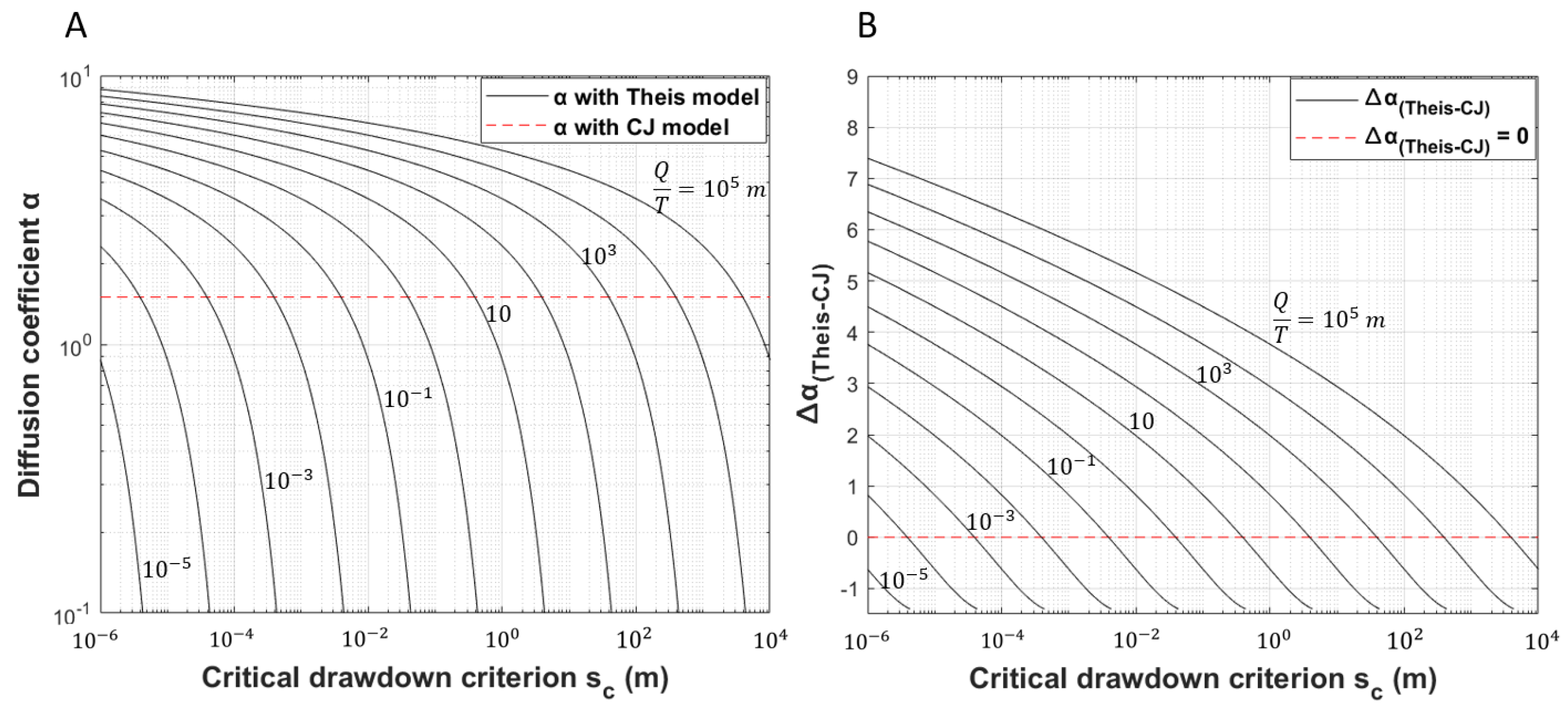
3.1. The Cooper Jacob Approximation (CJA) (1946) Approach

The approach based on the CJA considers the pressure front as the limit beyond which the drawdown is zero. The aquifer conceptual model of this approach derives from that of Theis, which assumes a two-dimensional groundwater flow occurring in a homogenous, isotropic medium of constant thickness with an infinite extension and the source has infinitesimal radius. The drawdown solution $s_{CJ}\left(r,t\right)$proposed by Cooper and Jacob [9] results from approximating the Theis well function to a straight-line for large dimensionless time. Chapuis [59] stated that the Cooper–Jacob approximation is tolerable for $u<0.01$; indeed, critical values equal to $0.02$ and $0.05$ are commonly practiced in hydrogeology applications [60,61,62].

Thus, taking Equation (10) and solving $s_{CJ}\left(r,t\right)=0$ leads to Equation (11), in which the diffusion coefficient value is $1.5$.

$$s_{CJ}\left(r,t\right)=\frac{Q}{4\pi T}ln\left(\frac{2.25Tt}{r^{2}S}\right)$$

(10)

$$r=1.5\sqrt{\frac{T}{S}t}$$

(11)

The advantage of the CJA approach is that it allows characterizing the diffusion equation by simply solving the equation$s_{CJ}\left(r,t\right)=0$. In addition, the fact that $\alpha =1.5$ is a constant is easier to implement by practitioners when calculating the distance of hydraulic objects. This value is also recommended by some hydrogeology manual [59]. However, the CJA approach is arbitrary because the value $\alpha =1.5$ induces an interpretation error of the pressure front. When the drawdown predicted by the CJ model is zero at the time $t_0$ (Figure 3), the drawdown predicted by the Theis model is equal to the critical value ${\epsilon }_{Theis-CJ}$ given by Equation (12).

This critical value, herein referred to as the pressure front interpretation error ${\epsilon }_{Theis-CJ}$, is proportional to $Q/T$ (in meters) and consequently becomes higher for low-transmissivity aquifers or high pumping rate hydraulic tests. The CJA approach also implicitly involves a greater error in the estimation of $\alpha$, in the sense that, if the pressure front is defined using the Theis drawdown model according to a variable criterion ${\mathrm{s}}_c$, the obtained $\alpha$ value given by Equation (13) might be higher or lesser than $1.5$, which refers to the CJ model (Figure 4A). The error of estimation of $\alpha$ with the CJ model, compared to that obtained with the Theis model ($\Delta {\alpha }_{Theis-CJ}$), is displayed in Figure 4B for different values of$Q/T$.

The minimum and maximum values of $Q/T$ are, respectively, ${10}^{-5}$ m and ${10}^5$m and are determined according to typical pumping test data obtained from communal and individual water-producing wells.

$${\epsilon }_{Theis-CJ}=s_{Theis}\left(r,t_0\right)=\frac{Q}{4\pi T}{E}_1\left(0.5625\right)=\frac{Q}{T}\ast 0.03903$$

(12)

$$\alpha =2\sqrt{E_1{}^{-1}\left(\frac{4\pi T}{Q}{s}_c\right)}$$

(13)

3.2. The Relative Critical Drawdown (RCD) Approach

The RCD approach is a method to characterize the diffusion equation that considers the pressure front criterion as the drawdown critical threshold ($s_c$), under which no disturbance generated by the pumping test is measurable. This criterion $s_c$ is quantified relative to the maximum drawdown at the pumping well $s\left(r_w,\Delta t\right)$ according to Equation (14) in which, $x$ is the relative factor ($x\in \left]0;1\right[$), $\Delta t$ is the total elapsed time of the pumping test and $r_w$ is the well radius [39,63]. Assuming the radial groundwater flow regime occurring under the Theis assumptions, the drawdown equation used to characterize the diffusion equation is given by Equation (15). Then, combing Equations (14) and (15) leads to Equation (16) [39].

$$s_c=x·s\left(r_w,\Delta t\right)$$

(14)

$$s_{Theis}\left(r,t\right)=\frac{Q}{4\pi T}{\mathrm{E}}_1\left(u\right) , u=\frac{r^{2}S}{4Tt}$$

(15)

$$r=\alpha \sqrt{\frac{T}{S}t} \mathrm{with} \alpha =2\sqrt{E_1{}^{-1}\left(x.{\mathrm{E}}_1\left(u_w\right)\right)} \mathrm{and} u_w=\frac{r_w{}^{2}S}{4T\Delta t}$$

(16)

Equation (16) shows that the diffusion coefficient $\alpha$ value depends on the pressure front relative factor $x$. Practically, Aguilera [64], Johnson [65] and Bourdarot [66], without providing any additional details, stated that Jones [35] defined the pressure front according to a relative factor of 1% and obtained Equation (18). Moreover, Hossain, Tamim and Rahman [57] quantified the pressure front relative factor at 0.0000016%, and they obtained Equation (17).

$$r=8.11\sqrt{\frac{T}{S}t}$$

(17)

$$=4\sqrt{\frac{T}{S}t}$$

(18)

The RCD approach makes it possible to characterize the diffusion equation both analytically and numerically. It is an exact approach because the diffusion coefficient $\alpha$ value is not constant and depends to the relative factor $x$, the aquifer hydraulic properties ($T$ and $S$), the total elapsed time $\Delta t$ and the well radius $r_w$. This gives the advantage of adapting the estimate of the diffusion coefficient value to the conditions under which the pumping test is conducted.

However, due to the fact that aquifer hydraulic properties could vary by several orders of magnitude depending on the nature of formations, the value of the diffusion coefficient could also vary widely. To ensure a certain stability of the diffusion coefficient value, the pressure front relative factor $x$ must also vary by several orders of magnitude, thus, leading to unrealistic definition of the pressure front in some practical cases.

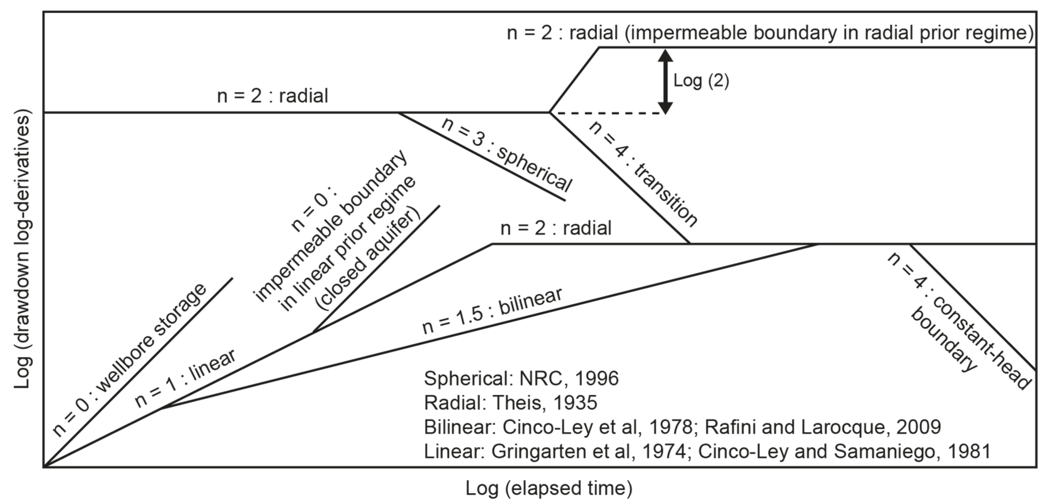
3.3. The Drawdown Log-Radius Derivative (DLRD) Approach

This approach characterizes the diffusion equation based on the drawdown log-radius derivative function Equation (19). The pressure front is defined at any distance where drawdown log-radius derivative reaches the absolute critical threshold $\delta$ such that $\delta \in \left[-\frac{Q}{2\pi T};0\right[$. Then, taking Equation (19) and solving $ds/dlnr=\delta$ leads to Equation (20).

$$\frac{d{s}_{Theis}\left(r,t\right)}{dln\left(r\right)}=-\frac{Q}{2\pi T}{e}^{-\frac{r^{2}S}{4Tt}}$$

(19)

$$r=\alpha \sqrt{\frac{T}{S}t} \mathrm{with} \alpha =2\sqrt{-\ln \left(\frac{-2\pi T}{Q}\delta \right)} \mathrm{and}-\frac{Q}{2\pi Kb}<\delta <0 \mathrm{and} \delta \mathrm{in} \mathrm{meter}$$

(20)

Equation (20) shows that the diffusion coefficient $\alpha$ depends on the pressure front criterion $\delta$, the pumping rate $Q$ and the aquifer transmissivity $T$, which give the advantage of the DLRD approach to adapt the value of the diffusion coefficient to the conditions under which the pumping test is conducted. For instance, Rahman et al. [37] proceeded by numerical simulations to determine the diffusion Equation (21). They arbitrarily estimated the pressure front criterion at $\left|\delta \right|=1 \mathrm{psi}$ (or $\left|\delta \right|=6894.76/\mathsf{\rho }\mathrm{g}$ in meters).

$$r=2.5495\sqrt{\frac{T}{S}t}$$

(21)

Although the DLRD approach has the advantage of better determining the value of the diffusion coefficient, it is not easy to put it into practice in a real pumping test case where drawdown time series data are recorded. Moreover, this approach is also subject to uncertainties in the definition of the pressure front as it is the case for the RCD approach, because the pumping rate $Q$, as well as the aquifer transmissivity $T$ could widely vary in realty.

3.4. The Relative Critical Flow (RCF) Approach

The RCF approach consists in defining the pressure front relatively to the fluid flow rate within the aquifer. During a pumping test, the propagation of the pressure disturbance induces a groundwater flow rate $q\left(r,t\right)$into the aquifer, which is analytically expressed by Equation (22) assuming the Theis conceptual model. This flow rate decreases as a function of the radial distance $r$ from the pumping well. The RCF approach considers the pressure front criterion as the flow rate critical threshold ($q_c$), under which no flow is measurable. The value of the criterion $q_c$ is quantified according to the pumping flow rate $Q$ at the source Equation (23). In this equation, $x$ is the relative factor such that$x\in \left]0;1\right[$. Then, combining Equations (22) and (23) leads to Equation (24).

$$q\left(r,t\right)=Q{e}^{-\frac{r^{2}S}{4Tt}}$$

(22)

$$q_c=xQ$$

(23)

$$r=\alpha \sqrt{\frac{T}{S}t} \mathrm{with} \alpha =2\sqrt{-\ln \left(x\right)}, x \in \left]0;1\right[$$

(24)

The diffusion coefficient $\alpha$ in Equation (24) depends only on the relative factor$x$. For instance, Tek, et al. [67] used the RCF approach to characterize the diffusion equation. They arbitrarily defined the pressure front according to a relative factor of 1%, leading to the following result:

$$r=4.29\sqrt{\frac{T}{S}t}$$

(25)

The fact that the diffusion coefficient from the RCF approach depends only on the relative factor $x$ makes this approach less restrictive than the RCD and DLRD approaches. As a result, using the RCF approach to calculated the distance of hydraulic objects may induce errors as this approach does not take into account the aquifer properties, the flow rate $Q$. In addition, the RCF approach is not easy to apply in the real-world context of a pumping test because it is not common to measure the fluid flow into the aquifer during transient hydraulic tests.

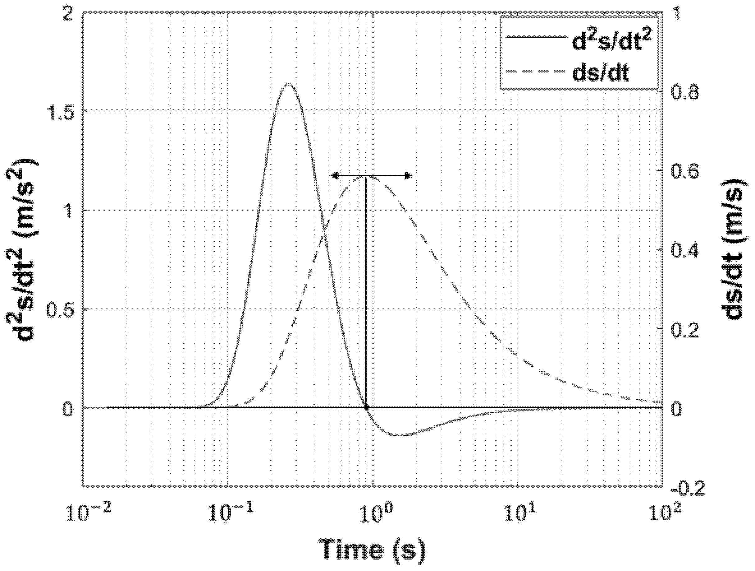
3.5. The Maximum Drawdown Rate (MDR) Approach

The maximum drawdown rate approach consists of characterizing the diffusion equation using the drawdown derivative function ($ds/dt$). This approach considers the pressure front as the pic of the $ds/dt$ function [66]. In other words, it finds the moment at which the second derivative of the drawdown function is zero ($d^{2}s/d{t}^2=0$) as illustrated on Figure 5. Assuming classic constant flow pumping test occurring in an aquifer formation that verifies the Theis hypothesis, the second derivative of the drawdown function $\frac{d^2{s}_{Theis}\left(r,t\right)}{d{t}^2}$ is given by Equation (26). Then, taking Equation (26) and setting it equal to zero leads to obtaining Equation (27).

$$\frac{d^2{s}_{Theis}\left(r,t\right)}{d{t}^2}=\frac{Q}{4\pi T}\left(u-1\right)\frac{e^{-u}}{t^2} \mathrm{with} u=\frac{r^{2}S}{4Tt}$$

(26)

$$r=2\sqrt{\frac{T}{S}t}$$

(27)

The MDR approach gives a physical meaning to the pressure front, which is the peak of the $ds/dt$ curve. Then, the diffusion coefficient that is obtained is a constant ($\alpha =2$) and does not depend on any parameter, such as the flow rate, the hydraulic properties, which makes the MDR approach subject to uncertainties. In other words, the fact that $\alpha$ is constant could induce some error of estimation of the distances of hydraulic objects.

3.6. The Maximum Drawdown (MD) Approach for an Impulse Test

The maximum drawdown (MD) approach uses the same principle as the maximum drawdown rate (MDR) method except that the MD approach directly relies on the drawdown function. Indeed, this approach considers the pressure front as the pic of the drawdown function for an impulse test. In other words, it determines the time at which the first derivative function of the drawdown is zero. To apply this approach, Lee [36] conceptualized a homogeneous and isotropic line source model with an infinite lateral extension. The drawdown solution ($s{\left(r,t\right)}_{GR}$) corresponding to these hypotheses for a pulse test is given by Equation (28) as proposed by Gringarten and Ramey [52].

$$s{\left(r,t\right)}_{GR}=\frac{S}{4\pi Tt}\exp \left(-\frac{r^{2}S}{4Tt}\right)$$

(28)

Equation (28) is similar to the first derivative of the drawdown solution predicted by the Theis model, which implies a long-time pumping test (LTPT). The relationship between both equations is given by Equation (29). This similarity is explained by the fact that a long-time constant flow rate pumping test (Theis hypothesis) is considered as an extension of a flow pulse test in the same conceptual model; thus, the drawdown produced by a LTPT is an integral of that produced by a pulse test [45,61].

Therefore, solving the diffusion problem with the flow pulse test by applying the maximum drawdown approach, i.e., $ds{\left(r,t\right)}_{GR}/dt=0$ [36], is equivalent to taking the second derivative of the Theis drawdown solution and setting it equal to zero ($d^{2}s{\left(r,t\right)}_{Theis}/d{t}^2=0$), as presented in the previous section (Section 3.5). Both approaches lead to the same result (see Equation (27)). Therefore, the MD approach could be subject to the same uncertainties related to the MDR approach as stated in the previous section.

$$s{\left(r,t\right)}_{GR}=\frac{S}{Q}\ast \frac{ds{\left(r,t\right)}_{Theis}}{dt}$$

(29)

3.7. The Deviation Time (DT) Approach

The concept of deviation time was introduced by Wattenbarger et al. [68] to refer to the time of influence of a hydraulic object in order to characterize its distance from the source during a transient hydraulic test. The time of influence is considered as the moment in time when a change in flow regime is judged significant enough to be detected on the drawdown signal. Wattenbarger et al. [68] simulated a long-time constant flow transient test in a vertical hydraulically fractured well whose fracture extends all the way to the lateral boundaries. The well is in the center of a rectangular drainage area as illustrated in Figure 6.

The flow regime that occurs is linear. The normalized drawdown solutions is given by Equation (30). Representing this equation on a bi-logarithmic scale shows a half-slope linear flow reflecting the natural behaviour of the aquifer, followed by a deviation illustrating the contribution of external boundaries to the aquifer hydrodynamics (Figure 7). Wattenbarger et al. [68] make a graphical approximation by stating that the deviation appears at $t_{Dye}=0.5$ without providing details on the precision with which the pressure front is read. Taking the expression of the parameter $t_{Dye}$, and setting it equal to $0.5$ leads to Equation (31).

$${\chi }^{-1}{s}_{wD}{}_{constant-flow}=\frac{1}{\rho g}\left[\frac{\pi }{2}\left[\frac{1}{3}+t_{Dye}\right]-\frac{2}{{\pi }^2}{\displaystyle \sum }_{n=1}^{\infty }\left(\frac{1}{n^2}\right)\exp \left[-n^2{\pi }^2{t}_{Dye}\right]\right]$$

(30)

where

$$\chi =\frac{y_e}{x_f}, t_{Dxf}=\frac{0.00633kt}{\varnothing \mu c_t{x}_f{}^2} , s_{wD}\left(r_w,t\right)=\frac{kb}{141.2qB\mu }s\left(r_w,t\right), t_{Dye}=\frac{0.00633kt}{\varnothing \mu c_t{y}_e{}^2}$$

$$r=1.42\sqrt{\frac{T}{S}{t}_{ehs}}$$

(31)

where $t_{ehs}$is considered by Wattenbarger et al. [68] as the time corresponding to the end of the half-slope ($ehs$) regime (Figure 7).

The value of the diffusion coefficient ($\alpha =1.42$) obtained by the DT approach for a constant flow rate is constant. This value depends on the accuracy with which Wattenbarger et al. [68] identified the value of the deviation time $t_{Dye}$. However, these authors did not provide details about this accuracy. Therefore, the DT approach may be subject to uncertainties in its application for the localisation of hydraulic objects.

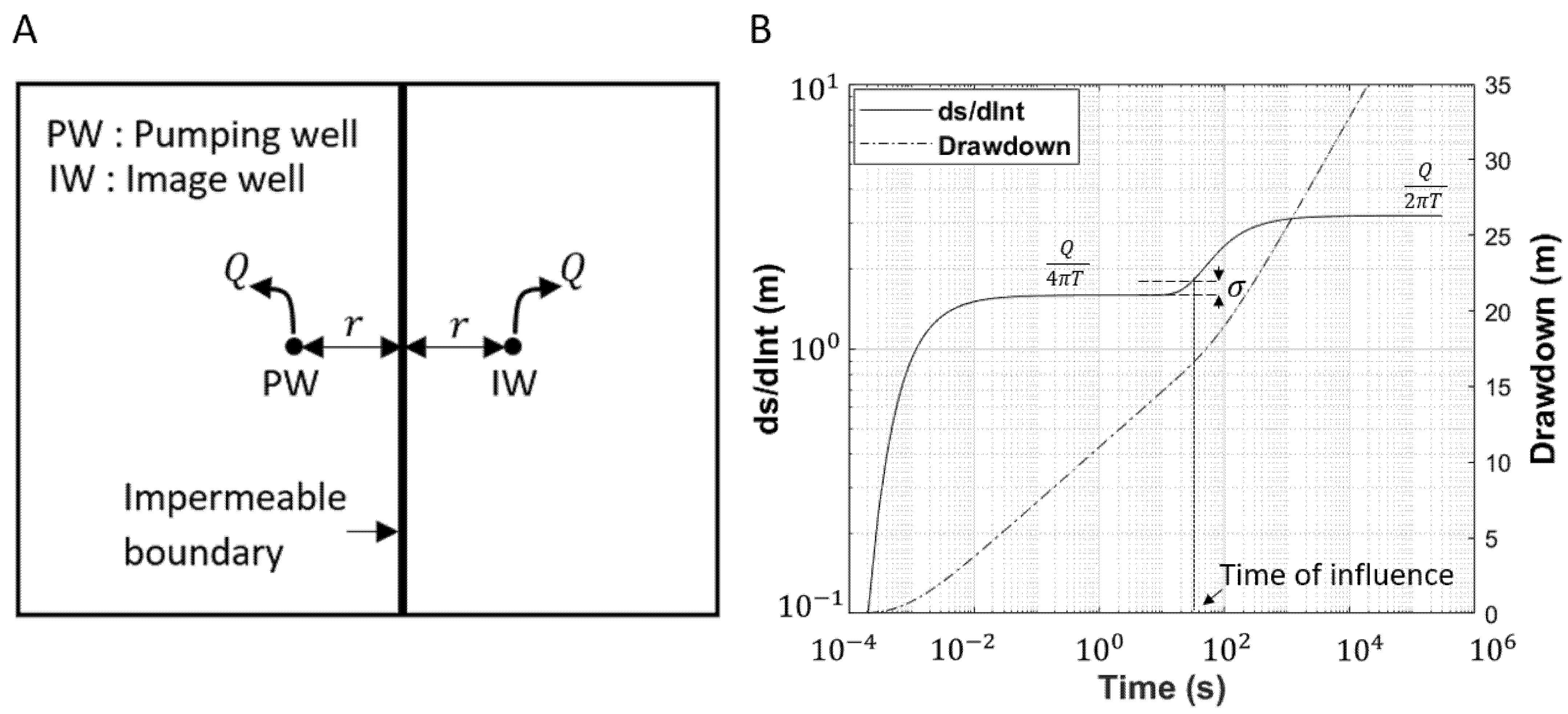
3.8. Developing a New Approach: The Drawdown Log-Time Derivative (DLTD) Approach

In addition to the methods presented in the previous Review section, a novel approach is proposed in this study to characterize the diffusion equation. We show that this new approach produces a more realistic diffusion coefficient value. The assumptions related to the Theis model are considered, i.e., the flow is two-dimensional and horizontal, occurring in a homogenous, isotropic medium of constant thickness with an infinite extension, and the source has an infinitesimal radius.

The DLTD approach is similar to the Wattenbarger approach and is applied to the Theis conceptual model, where the flow regime is radial. The objective is to characterise the diffusion equation from the influence of a hydraulic boundary—in our case, an impermeable boundary located at a distance $r$ from the source. The purpose of the approach is to determine the time of influence $t_i$ of the impermeable boundary on the drawdown log-derivative curve recorded at the pumping well. For this purpose, the “image-well” theory is applied, which considers an imaginary well to be located twice as far from the pumped well as the impermeable boundary (Figure 8A). The principle of the DLTD approach is first to determine the expressions of both the total drawdown produced into the real well $s_t\left(r_w,t\right)$ and its log-time derivative $d{s}_t\left(r_w,t\right)/dln\left(t\right)$.

Indeed, the total drawdown produced in the real well (Equation (32)) is the sum of that produced by the real well itself $s\left(r_w,t\right)$ and that produced by the imaginary well located at the distance ($2r$) from the real well $s\left(2r,t\right)$. Thus, the expression of the log-time derivative $d{s}_t\left(r_w,t\right)/dln\left(t\right)$ is given by Equation (33).

$$s_t\left(r_w,t\right)=\frac{Q}{4\pi T}\left[W\left(u_w\right)+W\left(u_{2r}\right)\right] with u_w=\frac{r_w{}^{2}S}{4Tt} and u_{2r}=\frac{{\left(2r\right)}^{2}S}{4Tt}$$

(32)

$$\frac{d{s}_t\left(r_w,t\right)}{dln\left(t\right)}=\frac{Q}{4\pi T}\left[\frac{d}{dln\left(t\right)}W\left(u_w\right)+\frac{d}{dln\left(t\right)}W\left(u_{2r}\right)\right] =\frac{Q}{4\pi T}\left[e^{-\frac{r_w{}^{2}S}{4Tt}}+e^{-\frac{{\left(2r\right)}^{2}S}{4Tt}}\right]$$

(33)

Both drawdown and log-time derivative signals are represented in Figure 8B. The time of influence ($t_i$) can be defined as the time at which the influence of the impermeable boundary starts to be felt in the real well. Then, in long time periods before the influence of the impermeable boundary is felt in the real well ($t<t_i$), the natural behaviour of the aquifer dominates; thus, the term $e^{-\frac{{\left(2r\right)}^{2}S}{4Tt}}$ becomes negligible and $e^{-\frac{r_w{}^{2}S}{4Tt}}\to 1$.

Therefore, Equation (33) simplifies to Equation (34), which illustrates the first plateau of the log-time derivative curve corresponding to the value $Q/\left(4\pi T\right)$ in Figure 8B. The value $Q/4\pi T$ corresponds to the slope of the Cooper–Jacob drawdown straight-line in semi-logarithmic scale.

In very long time periods, after the influence of the impermeable boundary is felt in the real well ($t\gg t_i$), $e^{-\frac{r_w{}^{2}S}{4Tt}}\to 1$and $e^{-\frac{{\left(2r\right)}^{2}S}{4Tt}}\to 1$, then Equation (33) simplifies to Equation (35), which corroborates the second plateau corresponding to the value $Q/\left(2\pi T\right)$. This value is equal to two times the Cooper–Jacob slope.

$$\frac{d{s}_t\left(r_w,t\right)}{dln\left(t\right)}=\frac{Q}{4\pi T} ; t<t_i$$

(34)

$$\frac{d{s}_t\left(r_w,t\right)}{dln\left(t\right)}=\frac{Q}{2\pi T} ; t\gg t_i$$

(35)

The time of influence $t_i$ of the impermeable boundary reflects the time at which a deviation from the natural behaviour of the aquifer is observed on the log-time derivative curve. This time of influence depends on the accuracy with which the deviation is interpreted. Indeed, if we consider the absolute criterion $\sigma$ (deviation of the $ds/dlnt$ curve with respect to the first plateau), it is then possible to characterise the distance of the impermeable boundary Equation (36) by solving$\frac{ds}{dlnt}=\frac{Q}{4\pi T}+\sigma$ (Figure 8B).

$$r=\alpha \sqrt{\frac{T}{S}{t}_i} with \alpha =\sqrt{-\ln \left(\frac{4\pi T}{Q}\sigma \right)} and 0<\sigma <\frac{Q}{4\pi T}$$

(36)

The diffusion coefficient obtained with the DLTD approach depends on both the criterion $\sigma$ at which the time of influence of the hydraulic boundary is determined, the aquifer transmissivity $T$ and the pumping flow rate $Q$. The knowledge of these parameters makes it possible to accurately determine the location of a hydraulic object using Equation (36). This approach is simpler and more practical, as it is based directly on the drawdown logarithmic derivative curve, which is usually employed by hydrogeologists to interpret pumping test data. However, due to the noise of the real pumping test data, the application of the DLTD approach to locate hydraulic objects may be subject to uncertainties.

Finally, the highlights of the seven approaches revised from the literature as well as the one developed in this paper are summarized in

Table 1. Summary of the relevant points of the different approaches.

Approaches and Definition of the Pressure Front	Pressure Front General Criteria and/or Expression of the Diffusion Coefficient $\mathit{\alpha }$	Pressure Front Specific Criteria	$\mathbf{Value} \mathbf{of} \mathit{\alpha }$	Hydraulic Test Condition	Flow Regimes	Authors
The Cooper Jacob Approximation (CJA) Approach: For any position $r$, the pressure front corresponds to the time when the drawdown predicted by the CJ model is zero.	$s{\left(r,t\right)}_{CJ}=0$ $s{\left(r,t\right)}_{CJ}=\frac{Q}{4\pi T}\ln \left(\frac{2.25Tt}{r^{2}S}\right)$	$s_c=0$	$1.5$	Constant flow rate drawdown test	Radial	[9]
The Relative Critical Drawdown (RCD) Approach: At any time $t$, the pressure front is defined at the position $r$, where the drawdown reaches a certain percentage $x$ of the total drawdown at the source.	$s_c=x.s\left(r_w,\Delta t\right)$ $\alpha =2\sqrt{E_1{}^{-1}\left(x.{\mathrm{E}}_1\left(u_w\right)\right)}$	$x=1\%$	$4$	Constant flow rate drawdown test	Radial	[35]
		$x=1.6·{10}^{-6}\%$	$8.11$	Constant flow rate drawdown test	Radial	[57]
The Drawdown Log-Radius Derivative (DLRD) Approach: At any time $t$, the pressure front is defined at the distance $r$, where the drawdown log-radius derivative reaches the absolute criterion $\delta$.	$\frac{\mathrm{ds}}{\mathrm{dln}\left(\mathrm{r}\right)}=\delta$ $\alpha =2\sqrt{-ln\left(\frac{-2\pi T}{Q}\delta \right)}$ $with-\frac{Q}{2\pi T}<\delta <0$	$\left|\delta \right|=1 \mathrm{psi}$	$2.5495$	Constant flow rate drawdown test	Radial	[37]
The Relative Critical Flow (RCF) Approach: At any time $t$, the pressure front is defined at the distance $r$, where the fluid flow reaches a certain percentage of the pumping flow rate at the source.	$q\left(r,t\right)=xQ$ $\alpha =2\sqrt{-ln\left(x\right)}$	$x=1\%$	$4.29$	Constant flow rate drawdown test	Radial	[67]
The Maximum Drawdown Rate (MDR) Approach: At any distance $r$ the pressure front is defined at the time $t$ when the pressure variation rate is maximum.	$\frac{d^{2}s\left(r,t\right)}{d{t}^2}=0$	$\frac{d^{2}s\left(r,t\right)}{d{t}^2}=0$	$2$	Constant flow rate drawdown test	Radial	[66]
The Maximum Drawdown (MD) Approach: At any distance $r$ the pressure front is defined at the time $t$ when the pressure disturbance is maximum.	$\frac{ds\left(r,t\right)}{dt}=0$	$\frac{ds\left(r,t\right)}{dt}=0$	$2$	Flow impulse test (injection)	Radial	[36]
The Deviation Time (DT) Approach: The pressure front is defined at the dimensionless time when a deviation is observed on the normalized drawdown curve.	Starting of the deviation	$t_{Dye}=0.5$	$1.414$	Constant flow rate drawdown test	Linear	[68]
The Drawdown Log-Time Derivative (DLTD) Approach: The pressure front is defined at the time when the deviation on the drawdown log-derivative curve reaches the absolute criterion $\sigma$.	$\frac{ds}{dln\left(t\right)}=\sigma$ $\alpha =2\sqrt{-ln\left(\frac{4\pi T}{Q}\sigma \right)}$ $0<\sigma <\frac{Q}{4\pi T}$			Constant flow rate drawdown test	Radial	This work

. For each approach, the pressure front criterion, the general expression of the diffusion coefficient $\alpha$, the specific pressure front criterion (if applicable), the different values of $\alpha$, the hydraulic test conditions, the flow regime and the names of the authors are mentioned. The approaches appear in the same order as they were discussed in the main body of the article.

In the end, all approaches summarised in Table 1 are based on the definition of the pressure front from theoretical criteria that use mathematical tools often difficult to access for practising hydrogeologists (DLRD, MDR and MD approaches). Sometimes these pressure front criteria are based on theoretical quantities that are difficult to measure in the field, such as the critical flow rate $q_c$ (the RCF approach). These different theoretical criteria make it difficult to implement the different approaches developed in real contexts of pumping test interpretation excepted those based on the critical drawdown values (CJA and RCD approaches) and the absolute criterion of the drawdown logarithmic derivative (the DLTD approach).

For this reason, we decided to convert all criteria into terms of critical drawdowns excepted the deviation time (DT) approach as it is based on a graphic determination of the parameter $t_{Dye}$. In other words, it is a matter of determining the equivalent critical drawdown value $s_{ceq}$ of each criterion. The different steps, as well as the results of this standardization, are summarized in

Table 2. Standardization of the criteria used in the different methods. (The steps 1 to 5 indicate the operation used to standardize the criteria of the different approaches).

Approaches	Initial Criteria		Equivalent Critical Drawdown Criteria	Authors
Standardization Step 1: Summary of different approaches	Standardization Step 2: Determining the expression of the pressure front criteria	Standardization Step 3: Combining the pressure front criteria in step 1 and their expressions given in step 2 leads to obtaining the expression of the parameter $u$	Standardization Step 4: Introducing the expression of the parameter u into the drawdown solution leads to the equivalent critical drawdown criterion
The Cooper Jacob Approximation (CJA) Approach	$s{\left(r,t\right)}_{CJ}=\frac{Q}{4\pi T}\ln \left(\frac{0.5625}{u}\right)$ $with u=\frac{r^{2}S}{4Tt}$	$s{\left(r,t\right)}_{CJ}=0 \to u=0.5625$	$s\left(u\right)=\frac{Q}{4\pi T}{E}_1\left(u\right)$ $s_{c_{eq}}=\frac{Q}{T}0.03903$	[9]
The relative critical drawdown (RCD) Approach	$s_c=x.\frac{Q}{4\pi T}{E}_1\left(\frac{r_w{}^{2}S}{4T\Delta t}\right)$ $with 0<x<1$	$s\left(r,t\right)=s_c \to$ $u=E_1{}^{-1}\left(x.E_1\left(\frac{r_w{}^{2}S}{4T\Delta t}\right)\right)$	$s\left(u\right)=\frac{Q}{4\pi T}{E}_1\left(u\right)$ $s_{c_{eq}}=0.07958x\frac{Q}{T}{E}_1\left(\frac{r_w{}^{2}S}{4T\Delta t}\right)$	[35,57,69]
The Drawdown Log-Radius Derivative (DLRD) Approach	$\frac{ds}{dln\left(r\right)}=-\frac{Q}{2\pi T}{e}^{-u}$ $with u=\frac{r^{2}S}{4Tt}$	$\frac{ds}{dln\left(r\right)}=\delta \to$ $u=-\ln \left(-\frac{2\pi T}{Q}\delta \right)$ $with-\frac{Q}{2\pi T}<\delta <0$	$s\left(u\right)=\frac{Q}{4\pi T}{E}_1\left(u\right)$ $s_{c_{eq}}=0.07958\frac{Q}{T}{E}_1\left(ln\left(-\frac{Q}{2\pi T\delta }\right)\right)$	[37]
The Relative Critical Flow (RCF) Approach	$x=e^{-u}$ $with u=\frac{r^{2}S}{4Tt}$	$x=e^{-u} \to$ $u=-\ln \left(x\right)$ $with 0<x<1$	$s\left(u\right)=\frac{Q}{4\pi T}{E}_1\left(u\right)$ $s_{c_{eq}}=0.07958\frac{Q}{T}{E}_1\left(ln\left(\frac{1}{x}\right)\right)$	[67]
The Maximum Drawdown Rate (MDR) Approach	$\frac{d^{2}s\left(r,t\right)}{d{t}^2}=\frac{Q}{4\pi T}\left(u-1\right)\frac{e^{-u}}{t^2}$ $with u=\frac{r^{2}S}{4Tt}$	$\frac{d^{2}s\left(r,t\right)}{d{t}^2}=0 \to$ $u=1$	$s\left(u\right)=\frac{Q}{4\pi T}{E}_1\left(u\right)$ $s_{c_{eq}}=\frac{Q}{4\pi T}{E}_1\left(1\right)=0.0176\frac{Q}{T}$	[66]
The Maximum Drawdown (MD) Approach	$\frac{ds\left(r,t\right)}{dt}=\frac{S}{4\pi T}\left(u-1\right)\frac{e^{-u}}{t^2}$ $with u=\frac{r^{2}S}{4Tt}$	$\frac{ds\left(r,t\right)}{dt}=0 \to$ $u=1$	$s\left(u\right)=\frac{S}{4\pi Tt}\exp \left(-u\right)$ $s_{c_{eq}}=\frac{1}{\pi e{r}^2}=\frac{0.117}{r^2}$	[36]
The Drawdown Log-Time Derivative (DLTD) Approach	$\frac{ds}{dln\left(t\right)}=\frac{Q}{4\pi T}{e}^{-u}$ $with u=\frac{r^{2}S}{4Tt}$	$\frac{ds}{dln\left(t\right)}=\sigma \to$ $u=-\ln \left(\frac{4\pi T}{Q}\sigma \right)$ $with 0<\sigma <\frac{Q}{4\pi T}$	$s\left(u\right)=\frac{Q}{4\pi T}{E}_1\left(u\right)$ $s_{c_{eq}}=0.07958\frac{Q}{T}{E}_1\left(ln\left(\frac{Q}{4\pi T\sigma }\right)\right)$	This work

.

4. Discussion and Conclusions

The diffusion equation is important in hydrogeology to locate hydraulic objects (around the pumping well) that can modify the hydrodynamics of aquifers. The objective of this paper is to review seven approaches developed by many authors to characterize the diffusion equation. The majority of these approaches characterize the diffusion equation directly according to a critical detectability criterion of the pressure front pulse, except for the approach of Wattenbarger et al. [68], which is based on the analytic resolution of conceptual flow problems involving a change in flow conditions due to a distant hydraulic object.

In addition to the seven approaches, a new one was developed in this article (the DLTD approach). This is similar to the Wattenbarger approach but adapted to the conceptual model of radial flow. The newly developed approach has the advantage of being both practical and rigorous. On the one hand, it is based on the logarithmic derivative curve usually used by practitioners for the interpretation of pumping tests.

On the other hand, the resulting diffusion coefficient considers the pressure front criterion $\sigma$, the aquifer transmissivity $T$ and the pumping flow rate $Q$, which is also the case of the RCD, DLRD and RCF approaches. It is worth remembering that the procedure for characterizing the diffusion equation from the Wattenbarger approach is indeed identical to that of the approach developed in this paper (the DLTD approach). However, it remains arbitrary and open to errors of interpretation as the authors do not mention the accuracy at which the pressure front is defined.

In addition, some approaches result in constant values of the diffusion coefficient. These approaches are subject to errors of interpretation, especially when applied to the calculation of distances of hydraulic objects, as they do not take into account certain variables ($Q$, $T$) that may affect the estimation of distances. This is the case for the CJA, MD and MDR approaches.

All the approaches presented in this review paper are subject to uncertainties in their application depending on the parameters taken into account in the estimation of the diffusion coefficient $\alpha$. Moreover, their application is strictly limited to the particular contexts of the flow regimes for which they were developed, i.e., the radial flow regime for most of them except for the DT approach, which corresponds to the linear regime.

Furthermore, all approaches are standardized, i.e., the criteria on which these approaches are based on are expressed in terms of critical drawdowns in order to compare them on the basis of the accuracy of the pressure front interpretation. However, in general, it appears that the equivalent critical drawdowns of certain approaches involve only the flow rate $Q$ and the transmissivity $T$. This is the case for the MDR and CJA approaches. Based on these criteria, the MDR approach can be said to be more accurate than the CJA approach. The other approaches involve other variables that make them non-comparable.

This scientific contribution, which consisted of rewriting the criteria for all approaches in terms of the critical drawdown, will allow the characterization of the diffusion equation to be studied more generally in the future. These future works will, therefore, serve to facilitate and more precisely determine the value of the diffusion coefficient and enable more appropriate use of the diffusion equation in the spatial interpretation of hydraulic objects.

References

1. Bridge, J.S.; Hyndman, D.W. Aquifer Characterization; Society for Sedimentary Geology: Tulsa, OK, USA, 2004; 172p. [Google Scholar]
2. Illman, W.A.; Zhu, J.; Craig, A.J.; Yin, D. Comparison of Aquifer Characterization Approaches through Steady State Groundwater Model Validation: A Controlled Laboratory Sandbox Study. Water Resour. Res. 2010, 46, W04502. [Google Scholar] [CrossRef]
3. Maliva, R.G. Aquifer Characterization Techniques; Springer: Cham, Switzerland, 2016; Volume 10. [Google Scholar]
4. Shishaye, H.A.; Tait, D.R.; Befus, K.M.; Maher, D.T. An Integrated Approach for Aquifer Characterization and Groundwater Productivity Evaluation in the Lake Haramaya Watershed, Ethiopia. Hydrogeol. J. 2019, 27, 2121–2136. [Google Scholar] [CrossRef]
5. Kabala, Z.J. The Dipole Flow Test: A New Single-borehole Test for Aquifer Characterization. Water Resour. Res. 1993, 29, 99–107. [Google Scholar] [CrossRef]
6. Gernand, J.D.; Heidtman, J.P. Detailed Pumping Test to Characterize a Fractured Bedrock Aquifer. Groundwater 1997, 35, 632–637. [Google Scholar] [CrossRef]
7. Vouillamoz, J.-M.; Favreau, G.; Massuel, S.; Boucher, M.; Nazoumou, Y.; Legchenko, A. Contribution of Magnetic Resonance Sounding to Aquifer Characterization and Recharge Estimate in Semiarid Niger. J. Appl. Geophys. 2008, 64, 99–108. [Google Scholar] [CrossRef]
8. Theis, C.V. The relation between the lowering of the Piezometric surface and the rate and duration of discharge of a well using ground-water storage. Trans. Am. Geophys. Union 1935, 16, 519–524. [Google Scholar] [CrossRef]
9. Cooper, H.H., Jr.; Jacob, C.E. A generalized graphical method for evaluating formation constants and summarizing well-field history. Eos Trans. Am. Geophys. Union 1946, 27, 526–534. [Google Scholar] [CrossRef]
10. Le Borgne, T.; Bour, O.; De Dreuzy, J.R.; Davy, P.; Touchard, F. Equivalent mean flow models for fractured aquifers: Insights from a pumping tests scaling interpretation. Water Resour. Res. 2004, 40. [Google Scholar] [CrossRef]
11. Bernard, S.; Delay, F.; Porel, G. A new method of data inversion for the identification of fractal characteristics and homogenization scale from hydraulic pumping tests in fractured aquifers. J. Hydrol. 2006, 328, 647–658. [Google Scholar] [CrossRef]
12. Rafini, S.; Larocque, M. Insights from numerical modeling on the hydrodynamics of non-radial flow in faulted media. Adv. Water Resour. 2009, 32, 1170–1179. [Google Scholar] [CrossRef]
13. Rafini, S.; Chesnaux, R.; Ferroud, A. A numerical investigation of pumping-test responses from contiguous aquifers. Appl. Hydrogeol. 2017, 25, 877–894. [Google Scholar] [CrossRef]
14. Ferroud, A.; Chesnaux, R.; Rafini, S. Insights on pumping well interpretation from flow dimension analysis: The learnings of a multi-context field database. J. Hydrol. 2018, 556, 449–474. [Google Scholar] [CrossRef] [Green Version]
15. Leveinen, J. Composite model with fractional flow dimensions for well test analysis in fractured rocks. J. Hydrol. 2000, 234, 116–141. [Google Scholar] [CrossRef]
16. Kuusela-Lahtinen, A.; Niemi, A.; Luukkonen, A. Flow Dimension as an Indicator of Hydraulic Behavior in Site Characterization of Fractured Rock. Groundwater 2003, 41, 333–341. [Google Scholar] [CrossRef] [PubMed]
17. Lods, G.; Gouze, P. WTFM, software for well test analysis in fractured media combining fractional flow with double porosity and leakance approaches. Comput. Geosci. 2004, 30, 937–947. [Google Scholar] [CrossRef]
18. Maréchal, J.-C.; Dewandel, B.; Subrahmanyam, K. Use of hydraulic tests at different scales to characterize fracture network properties in the weathered-fractured layer of a hard rock aquifer. Water Resour. Res. 2004, 40. [Google Scholar] [CrossRef] [Green Version]
19. Audouin, O.; Bodin, J.; Porel, G.; et Bourbiaux, B. Flowpath structure in a limestone aquifer: Multi-borehole logging investigations at the hydrogeological experimental site of Poitiers, France. Hydrogeol. J. 2008, 16, 939–950. [Google Scholar] [CrossRef]
20. Verbovšek, T. Influences of Aquifer Properties on Flow Dimensions in Dolomites. Groundwater 2009, 47, 660–668. [Google Scholar] [CrossRef]
21. Odling, N.; West, L.; Hartmann, S.; Kilpatrick, A. Fractional flow in fractured chalk; A flow and tracer test revisited. J. Contam. Hydrol. 2013, 147, 96–111. [Google Scholar] [CrossRef] [Green Version]
22. Chow, V.T. On the determination of transmissibility and storage coefficients from pumping test data. Trans. Am. Geophys. Union 1952, 33, 397–404. [Google Scholar] [CrossRef] [Green Version]
23. Tiab, D.; Kumar, A. Application of the PD’Function to Interference Analysis. J. Pet Technol 1980, 32, 1465–1470. [Google Scholar] [CrossRef]
24. Bourdet, D.; Whittle, T.M.; Douglas, A.A.; et Pirard, Y.M. A new set of type curves simplifies well test analysis. World Oil 1983, 196, 95–106. [Google Scholar]
25. Renard, P.; Glenz, D.; Mejias, M. Understanding diagnostic plots for well-test interpretation. Appl. Hydrogeol. 2008, 17, 589–600. [Google Scholar] [CrossRef] [Green Version]
26. Barker, J.A. A generalized radial flow model for hydraulic tests in fractured rock. Water Resour. Res. 1988, 24, 1796–1804. [Google Scholar] [CrossRef] [Green Version]
27. Issaka, M.; Ambastha, A. A Generalized Pressure Derivative Analysis For Composite Reservoirs. J. Can. Pet. Technol. 1999, 38. [Google Scholar] [CrossRef]
28. Beauheim, R.L.; et Roberts, R.M. Flow-dimension analysis of hydraulic tests to characterize water-conducting features. In Dans Water-Conducting Features in Radionuclide Migration, GEOTRAP Project Workshop Proceedings, Barcelona, Spain, 10–12 June 1998; OECD NEA: Paris, France, 1998; pp. 287–294. ISBN 92-64-17124X. [Google Scholar]
29. Bowman, D.O.; Roberts, R.M.; Holt, R.M. Generalized Radial Flow in Synthetic Flow Systems. Groundwater 2012, 51, 768–774. [Google Scholar] [CrossRef]
30. Ferroud, A.; Rafini, S.; Chesnaux, R. Using flow dimension sequences to interpret non-uniform aquifers with constant-rate pumping-tests: A review. J. Hydrol. X 2018, 2, 100003. [Google Scholar] [CrossRef]
31. Doe, T. Fractional dimension analysis of constant-pressure well tests. In Proceedings of the Dans SPE Annual Technical Conference and Exhibition, Dallas, TX, USA, 6–9 October 1991; Society of Petroleum Engineers. Paper No. SPE-22702-MS. pp. 461–467. [Google Scholar] [CrossRef]
32. Chesnaux, R. Avoiding confusion between pressure front pulse displacement and groundwater displacement: Illustration with the pumping test in a confined aquifer. Hydrol. Process. 2018, 32, 3689–3694. [Google Scholar] [CrossRef]
33. Rafini, S.; Larocque, M. Numerical modeling of the hydraulic signatures of horizontal and inclined faults. Appl. Hydrogeol. 2012, 20, 337–350. [Google Scholar] [CrossRef]
34. Muskat, M. The Flow of Homogeneous Fluids through Porous Media: Analogies with Other Physical Problems; McGraw-Hill Incorporated: New York, NY, USA, 1937. [Google Scholar]
35. Jones, P. Reservoir Limit Test on Gas Wells. J. Pet. Technol. 1962, 14, 613–619. [Google Scholar] [CrossRef]
36. Lee, J. Well Testing; Society of Petroleum Engineers of AIME: Dallas, TX, USA, 1982; 159p. [Google Scholar]
37. Rahman, N.M.A.; Pooladi-Darvish, M.; Santo, M.S.; Mattar, L. Use of PITA for Estimating Key Reservoir Parameters. J. Can. Pet. Technol. 2008, 47, PETSOC-08-08-24. [Google Scholar] [CrossRef]
38. Horner, D.R. Pressure Build-up in Wells.; World Petroleum Congress. Available online: https://onepetro.org/WPCONGRESS/proceedings-abstract/WPC03/All-WPC03/WPC-4135/203521 (accessed on 27 February 2022).
39. Bresciani, E.; Shandilya, R.N.; Kang, P.K.; Lee, S. Well radius of influence and radius of investigation: What exactly are they and how to estimate them? J. Hydrol. 2020, 583, 124646. [Google Scholar] [CrossRef]
40. Chang, J.; Yortsos, Y.C. Pressure-Transient Analysis of Fractal Reservoirs. SPE Form. Eval. 1990, 5, 31–38. [Google Scholar] [CrossRef]
41. Acuna, J.A.; Yortsos, Y.C. Application of Fractal Geometry to the Study of Networks of Fractures and Their Pressure Transient. Water Resour. Res. 1995, 31, 527–540. [Google Scholar] [CrossRef]
42. Cello, P.A.; Walker, D.D.; Valocchi, A.; Loftis, B. Flow Dimension and Anomalous Diffusion of Aquifer Tests in Fracture Networks. Vadose Zone J. 2009, 8, 258–268. [Google Scholar] [CrossRef] [Green Version]
43. Brixel, B.; Klepikova, M.; Lei, Q.; Roques, C.; Jalali, M.R.; Krietsch, H.; Loew, S. Tracking Fluid Flow in Shallow Crustal Fault Zones: Insights From Cross-Hole Forced Flow Experiments in Damage Zones. J. Geophys. Res. Solid Earth 2020, 125. [Google Scholar] [CrossRef]
44. Walker, D.D.; Cello, P.A.; Valocchi, A.J.; Loftis, B. Flow dimensions corresponding to stochastic models of heterogeneous transmissivity. Geophys. Res. Lett. 2006, 33. [Google Scholar] [CrossRef] [Green Version]
45. Nicol, A.; Walsh, J.; Watterson, J.; Gillespie, P. Fault size distributions—Are they really power-law? J. Struct. Geol. 1996, 18, 191–197. [Google Scholar] [CrossRef]
46. Hardacre, K.; Cowie, P. Variability in fault size scaling due to rock strength heterogeneity: A finite element investigation. J. Struct. Geol. 2003, 25, 1735–1750. [Google Scholar] [CrossRef]
47. de Dreuzy, J.-R.; Davy, P.; Erhel, J.; D’Ars, J.D.B. Anomalous diffusion exponents in continuous two-dimensional multifractal media. Phys. Rev. E 2004, 70, 016306. [Google Scholar] [CrossRef] [Green Version]
48. De Dreuzy, J.-R.; Davy, P. Relation between fractional flow models and fractal or long-range 2-D permeability fields. Water Resour. Res. 2007, 43. [Google Scholar] [CrossRef] [Green Version]
49. Giese, M.; Reimann, T.; Liedl, R.; Maréchal, J.-C.; Sauter, M. Application of the flow dimension concept for numerical drawdown data analyses in mixed-flow karst systems. Appl. Hydrogeol. 2017, 25, 799–811. [Google Scholar] [CrossRef]
50. Datta-Gupta, A.; Xie, J.; Gupta, N.; King, M.J.; Lee, W.J. Radius of Investigation and its Generalization to Unconventional Reservoirs. J. Pet. Technol. 2011, 63, 52–55. [Google Scholar] [CrossRef]
51. Craig, D.P.; et Jackson, R.A. Calculating the Volume of Reservoir Investigated During a Fracture-Injection/Falloff Test DFIT. In Proceedings of the Dans SPE Hydraulic Fracturing Technology Conference and Exhibition, The Woodlands, TX, USA, 24 January 2017. Society of Petroleum Engineers. Paper No. SPE-184820-MS. [Google Scholar] [CrossRef]
52. Gringarten, A.C.; Ramey, H.J.J. The Use of Source and Green’s Functions in Solving Unsteady-Flow Problems in Reservoirs. Soc. Pet. Eng. J. 1973, 13, 285–296. [Google Scholar] [CrossRef]
53. Horne, R.N.; Temeng, K.O. Recognition and Location of Pinchout Boundaries by Pressure Transient Analysis. J. Pet. Technol. 1982, 34, 517–519. [Google Scholar] [CrossRef]
54. Alabert, F.G. Constraining description of randomly heterogeneous reservoirs to pressure test data: A Monte Carlo study. In Proceedings of the Dans SPE Annual Technical Conference and Exhibition, San Antonio, TX, USA, 8 October 1989. Society of Petroleum Engineers. Paper No. SPE-19600-MS. [Google Scholar] [CrossRef]
55. Bourdet, D. Well Test Analysis: The Use of Advanced Interpretation Models; Elsevier: New York, NY, USA, 2002; 426p. [Google Scholar]
56. Taheri, A.; Shadizadeh, S.R. Investigation of Well Drainage Geometries in One of the Iranian South Oil Fields; Paper No. PETSOC-2005-028; Petroleum Society of Canada: Calgary, AB, Canada, 2005. [Google Scholar]
57. Hossain, M.; Tamim, M.; Rahman, N. Effects of Criterion Values on Estimation of the Radius of Drainage and Stabilization Time. J. Can. Pet. Technol. 2007, 46, 24–30. [Google Scholar] [CrossRef]
58. Ferroud, A.; Chesnaux, R.; Rafini, S. Drawdown log-derived analysis for interpreting constant-rate pumping tests in inclined substratum aquifers. Appl. Hydrogeol. 2019, 27, 2279–2297. [Google Scholar] [CrossRef]
59. Chapuis, R.P. Guide des Essais de Pompage et Leurs Interprétations [Guide to Pumping Tests and Their Interpretation]; Gov. of Quebec: Quebec City, QC, Canada, 2007; 55p.
60. Ferris, J.G.; Knowles, D.B.; Brown, R.; et Stallman, R.W. Theory of Aquifer Tests; US Geological Survey Denver: Denver, CO, USA, 1962.
61. Todd, D.K.; et Mays, L.W.I. Groundwater Hydrology, 2nd ed.; John Willey&Sons: Hoboken, NJ, USA, 1980. [Google Scholar]
62. Todd, D.K.; et Mays, L.W. Groundwater Hydrology, 3rd ed.; John Wiley&Sons: Hoboken, NJ, USA, 2004. [Google Scholar]
63. Bird, R.B.; Stewart, W.E.; et Lightfoot, E.N. Transport Phenomena John; Department of Chemical Engineering, University of Wisconsin: Madison, WI, USA; John Wiley&Sons, Inc.: New York, NY, USA; London, UK, 1960. [Google Scholar]
64. Aguilera, R. Radius and linear distance of investigation and interconnected pore volume in naturally fractured reservoirs. J. Can. Pet. Technol. 2006, 45. [Google Scholar] [CrossRef]
65. Johnson, P.W. The Relationship Between Radius of Drainage and Cumulative Production (includes associated papers 18561 and 18601). SPE Form. Eval. 1988, 3, 267–270. [Google Scholar] [CrossRef]
66. Bourdarot, G. Well Testing: Interpretation Methods; Editions Technip: Paris, France, 1998; ISBN 2-7108-0738-6. [Google Scholar]
67. Tek, M.; Grove, M.; Poettmann, F. Method for Predicting the Back-Pressure Behavior of Low Permeability Natural Gas Wells. Trans. AIME 1957, 210, 302–309. [Google Scholar] [CrossRef]
68. Wattenbarger, R.A.; El-Banbi, A.H.; Villegas, M.E.; et Maggard, J.B. Production analysis of linear flow into fractured tight gas wells. In Proceedings of the Dans SPE Rocky Mountain Regional/Low-Permeability Reservoirs Symposium, Denver, CO, USA, 5–8 April 1998. Society of Petroleum Engineers. Paper No. SPE-39931-MS. [Google Scholar] [CrossRef]
69. Nobakht, M.; Clarkson, C.R.; et Kaviani, D. New and improved methods for performing rate-transient analysis of shale gas reservoirs. SPE Reserv. Eval. Eng. 2012, 15, 335–350. [Google Scholar] [CrossRef]
Figure 1. Summary of published theoretical flow regimes and their associated flow dimensions n in bi-log scale of d l o g s / d t vs. time (redrawn from [12]).
Geosciences 12 00201 g001
Figure 2. Examples of flow geometries for integer flow dimensions: (a) one-dimensional flow within a plane ( n = 1 and v = 1 / 2 ); and (b) two-dimensional flow within a cylinder (well) ( n = 2 , v = 0 ); and (c) three-dimensional flow within a sphere ( n 3 , v = 1 / 2 ).
Geosciences 12 00201 g002
Figure 3. Illustration of simulated drawdown curves predicted by Theis and CJ models at r = 6   m for a pumping test with Q = 0.2   m 3 / s , T = 0.01   m 2 / s and S = 0.001 .
Geosciences 12 00201 g003
Figure 4. (A)—Comparison of α values from Theis and CJ models; (B)—Representation of α estimation error of CJ model compared to α estimation from Theis model.
Geosciences 12 00201 g004
Figure 5. Representation of drawdown solution predicted by the Theis model and its first derivative functions versus time at the position r = 6   m , with Q = 0.18   m 3 / s , T = 0.01   m 2 / s and S = 0.001 .
Geosciences 12 00201 g005
Figure 6. Example of hydraulic fracture in the center of a rectangular reservoir.
Geosciences 12 00201 g006
Figure 7. Representation of the drawdown solution for constant rate pumping test in a closed linear reservoir (redrawn from [68]).
Geosciences 12 00201 g007
Figure 8. (A) Aquifer conceptual model with linear impermeable boundary. (B) Drawdown s ( r , t ) and log-derivative d s / d l n t curves.
Geosciences 12 00201 g008