Regional-Scale Seismic Liquefaction Susceptibility Mapping via an Empirical Approach Validated by Site-Specific Analyses

Abstract

Regional-scale analyses of susceptibility to liquefaction are seldom performed in data-scarce areas. However, in spite of data limitations, such efforts can still provide useful information in case of populated, seismically active regions. The present work focuses on susceptibility zonation for soil liquefaction that might occur due to ground shaking in the Foggia Province, a data-scarce, seismically active area of about 7000 km² located in southern Italy. The Analytical Hierarchy Process (AHP) approach is used to obtain the susceptibility to liquefaction map of the whole area, while a geological and geotechnical database including 531 boreholes from 84 localities is used for cross-validation. The data are processed by means of a simplified quantitative method to determine liquefaction potential and assess whether a specific area is prone to liquefaction or not. Our results, along with an AUC − ROC = 0.89 test value, indicate that there are widespread areas of medium to high and very high susceptibility, and that the most susceptible zones are localized along the Adriatic Sea coastline and watercourses. The final susceptibility to liquefaction map represents a step forward towards the assessment of secondary seismic hazard in the study area, thus supporting the regional and local administrations responsible for land-use planning and risk mitigation.

1. Introduction

Liquefaction represents an important indirect phenomenon capable to cause damage to buildings and infrastructure during an earthquake (e.g., [1]). Liquefaction hazard assessment is one of the relevant components of seismic risk analysis as well as risk mitigation planning [2,3,4,5,6].

Liquefaction has caused diffuse damage worldwide during major earthquakes events, such as in Alaska in 1964; Loma Prieta, California in 1989; Kobe, Japan in 1995; Chi-Chi, Taiwan in 1999; Perú in 2001; New Zealand 2010; and Sichuan, China in 2008 [6,7,8], to mention a few. This phenomenon occurs also on the European Continent, and in this regard [6], describes liquefaction associated with several earthquakes, i.e., Turkey 1999 and 2012 and Greece 2008 and 2014. In the Italian peninsula, liquefaction events have recently been reported during the 2009 Aquila (central Italy) earthquake [9] and the 2012 Emilia (northern Italy) earthquake [10,11].

Liquefaction is a typical secondary effect that occurs due to ground shaking and rapid increase of pore-water pressure with consequent reduction in soil shear strength [12,13,14,15,16,17]. Soils prone to liquefaction are mainly sands and silty sands, which change their state from solid to a viscous fluid mass, [3,14,18].

Different factors influence the occurrence of liquefaction, including local litho-stratigraphy, water table depth, which in turn depends on the existing hydraulic regimes and boundary conditions (e.g., distance to sea coast, rivers and streams, water feeding systems, topographic indicators), as well as regional seismicity [6,8,19]. These factors are spatially variable with their estimates being largely uncertain, so that compiling susceptibility liquefaction maps at regional scales could be a challenging task [20]. However, a liquefaction susceptibility map is essential to identify areas prone to liquefaction hazards in seismically-active regions. This is exemplified by a recent study of the liquefaction potential in Po Plain, Italy [21], where the vulnerability related to this phenomenon is described as an “unexpected vulnerability” to moderate magnitude earthquakes.

In their recent studies, [6,8,19,22] present global scale liquefaction models using datasets from many historical earthquakes. In particular, [8,19] propose a geospatial approach to estimate earthquake-induced liquefaction from geospatial explanatory variables, available at global scale, which are proxies for soil saturation, soil density, and dynamic loading. They propose one Global Geospatial Liquefaction Model (GGLM) for coastal earthquakes and another one for non-coastal earthquakes, relying on datasets from 27 earthquakes that occurred in United States, Japan, New Zealand, China, Taiwan, and India, with the majority of the liquefaction events localized in coastal areas. A statistical logistic regression approach is used to develop the model and susceptibility maps for two test areas ascribed to four earthquakes that occurred in Kobe (Japan) and Christchurch (New Zealand), where liquefaction and non-liquefactions polygons are spatially defined across each region. Subsequently, [6] introduce an upgrade of the model proposed by [8], aimed at the two specific goals. First, the authors test the Global Geospatial Liquefaction Model (GGLM), including an additional 29 new events not considered in [8], in order to evaluate the performance of the model at regional scale. Secondarily, they build the GGLM in order to develop a liquefaction intensity index. In addition, [12] propose a probabilistic model of liquefaction hazard and risk in Portugal to assess the expected damage on buildings at a national scale and demonstrate that several regions of Portugal are prone to liquefaction hazard.

Other recent studies have evaluated the performance of regional liquefaction maps by comparing predictive models with real cases of earthquake-induced liquefaction phenomena [20,23,24]. In particular, [20] create a mega-zonation map of earthquake-induced soil liquefaction hazard for the entire European area using a probabilistic prediction model based on a logistic regression function. The maps prepared for different return periods are calibrated and validated by using a database of liquefaction phenomena that occurred in Europe [25].

In data-scarce areas, knowledge-driven methods can represent a valid alternative to data-driven approaches to the assessment of susceptibility to earthquake-induced liquefaction. One of these methods is the Analytical Hierarchy Process (AHP), introduced by [26]. It is a multi-criteria decision analysis technique that has been successfully used in different natural hazard contexts [27]. The application examples include landslide susceptibility and risk analysis [28,29,30], as well as soil liquefaction potential assessment [7]. AHP is widely acknowledged as a powerful tool capable to reduce analysis errors in a data-scarce environment, or in cases of discontinuous data series (in time and/or space) [28,30].

The aim of this work is to present and describe a liquefaction susceptibility map of a data-scarce area of about 7000 km², located in southern Italy (Figure 1). Regarding the study area, archival information describes several episodes of liquefaction phenomena with reference to the historic earthquakes that occurred in the last few hundred years [31]. However, the scientific literature only provides extremely low-resolution information based on the estimates of liquefaction probability at the Italian [31] and European [20] scale, and no regional scale assessment of liquefaction potential exists for the study area. In addition, as it regards liquefaction damage potential, only local-scale information is available from the investigation of a coastal town located just to the of the study area [32].

To fill this gap, the authors first prepared a susceptibility to liquefaction map using the AHP heuristic method that does not consider a specific earthquake event but rather considers the intrinsic seismicity derived from the official PGA (Peak Ground Acceleration) and Vs₃₀ (the time-averaged shear-wave velocity to 30 m depth) national scale maps available for Italy. The susceptibility map is then cross-validated through a site-specific liquefaction analysis based on geotechnical parameters locally derived from SPT (standard penetration tests). Furthermore, in the attempt to estimate the uncertainty associated with the heuristic susceptibility analysis, the standard deviation of the obtained susceptibility potential is calculated at pixel level (50 × 50 m cell).

2. Study Area

The study area covers 7020 km² of the Foggia Province, which represents the northernmost sector of the administrative region of Apulia (southern Italy). From west to east, it includes the easternmost Apennine Mountains (also known as the Daunia Mountains), the plain Tavoliere delle Puglie, and the Gargano Promontory and the Adriatic Sea coastal areas (Figure 1). The Daunia Mountains include the Cretaceous-Miocene clayey and flyschoid rocks belonging to the Fortore Unit in the western sector and to the Daunia Unit in the eastern sector ([33,34] and references therein). The Tavoliere delle Puglie plain is characterized by Plio-Quaternary deposits slightly dipping towards NE, made out of Pliocene clays, silts and sands (Argille Sub-Appennine, [35]), and Quaternary continental conglomeratic-sandy deposits belonging to the Tavoliere delle Puglie supersyntem [34,36,37,38]. The northernmost part of the study site is represented by the Gargano Promontory, made out of carbonate platform units (e.g., Calcare di Bari, Calcare di Altamura, Calcari di Monte Acuto by Servizio Geologico d’Italia, [36]) of the Middle Jurassic and Upper Cretaceous age. Finally, Holocene eluvial, colluvial, and alluvial deposits outcrop broadly on the entire area.

The hydrography of the area is characterized by torrential streams, which drain the the Daunia Apennines and the Tavoliere delle Puglie plain into the Adriatic Sea. Except for the Candelaro Stream that borders the south-western edge of the Gargano Promontory and is characterized by a NW-SE trend (Figure 1), the streams in the plain have generally narrow, unconfined, and shallow riverbeds.

From the hydrogeological point of view, the literature reports the three main aquifers [39]. The first aquifer, which is geometrically higher, is present within the Quaternary deposits covering the Tavoliere delle Puglie [40]. The base of this aquifer water circulation coincides with the stratigraphic contact with the Argille SubAppenine [35], whose estimated depth in the Foggia area (Figure 1) is about 40 m below ground surface [38]. Furthermore, the piezometric heights of this aquifer decrease proceeding from SW towards NE, with a preferential flow direction towards NE [38,41]. In an intermediate position, at variable depths, there is the second aquifer, which is hosted within sandy-loamy and subordinately gravelly layers, characterizing the succession of the Argille Sub-Apennine [35]. Then, at greater depths, the deeper aquifer is hosted by the carbonate rocks of the Apulian Platform, characterized by considerable permeability due to karst fracturing [40].

Due to their geological, geotechnical, and hydrogeological properties, most of the Quaternary deposits cropping out in the area could be involved in liquefaction phenomena. Indeed, the Historical seismic catalogue (e.g., Parametric Catalogue of Italian Earthquakes—CPTI15 version 4.0 released by INGV, Rome, Italy; see Figure 1 and

Table 1. Earthquakes with a magnitude greater than 5. Data from the historical seismic catalogue (Parametric Catalogue of Italian Earthquakes—CPTI15 version 4.0 released by INGV. From [42,43].

Year	Site	Magnitude
1627	Capitanata	Mw 6.66 ± 0.10
1361	Subappennino Dauno	Mw 6.03 ± 0.46
1627	Capitanata	Mw 5.80 ± 0.46
1627	Capitanata	Mw 6.03 ± 0.46
1646	Gargano	Mw 6.72 ± 0.25
1657	Capitanata	Mw 5.96 ± 0.15
1731	Tavoliere delle Puglie	Mw 6.33 ± 0.13
1857	Capitanata	Mw 5.86 ± 0.12

) reports that the study area was affected in the past by medium to high magnitude earthquakes.

The most relevant earthquakes (Table 1) originate from NW-SE oriented extensional tectonic structures present in the subsurface of the Tavoliere delle Puglie and from E-W strike-slip or oblique faults that cross the Gargano Promontory ([44,45] and references therein). Therefore, the exposure of the study area to seismic events with a magnitude greater than 5, together with the lithostratigraphic and hydrogeological setting, determine conditions favourable for the occurrence of liquefaction phenomena [46]. This gives rise, in particular, in the Tavoliere delle Puglie sector, to a high liquefaction potential [20,47] confirmed also by the historically documented soil liquefaction events (Figure 1) [47,48,49,50].

Figure 1. Simplified structural and lithological map of the study area; location in southern Italy indicated in inset by blue square. The capable faults are from ITHACA Catalogue (ITaly HAzards from CApable faulting [44]) and major (Mw ≥ 5.0) historical and instrumental earthquakes are from Rovida [42,43]). Green stars show the main cases of soil liquefaction induced by historical earthquakes (from [49]).

Figure 1. Simplified structural and lithological map of the study area; location in southern Italy indicated in inset by blue square. The capable faults are from ITHACA Catalogue (ITaly HAzards from CApable faulting [44]) and major (Mw ≥ 5.0) historical and instrumental earthquakes are from Rovida [42,43]). Green stars show the main cases of soil liquefaction induced by historical earthquakes (from [49]).

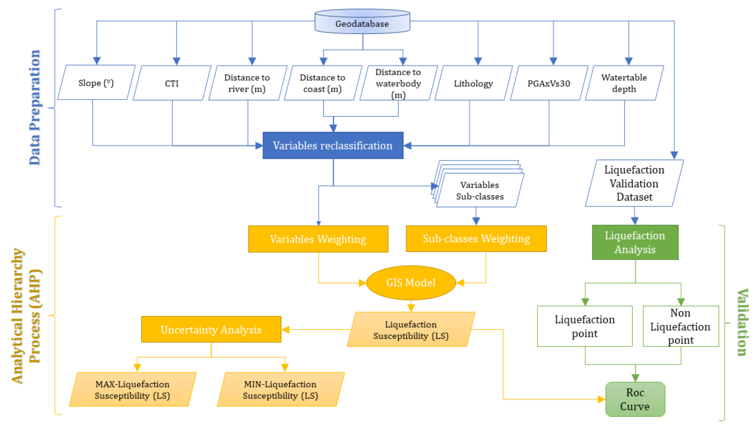
3. Susceptibility Model

The aim of the susceptibility analysis proposed is to identify zones with significantly higher probability of liquefaction potential under seismic triggering conditions in an area characterized by scarce historical records of occurrence.

There is evidence that at least one earthquake, whichoccurred in 1627, produced liquefaction phenomena in several sites of the study area (Figure 1; [48,49]). No additional specific information is available in the recently updated Italian Catalogue of Earthquake Induced Failure [49,51,52] accessible at https://gdb.ceri.uniroma1.it/index.php/view/map/?repository=cedit&project=Cedit (accessed on 12 April 2022). The catalogue compiles different types of secondary effects associated with earthquakes, including liquefaction, landslides, and surface faulting. Considering that several historic earthquakes with M > 5 originated in the study area (Table 1), it is possible that some instances of liquefaction phenomena might have not been recorded or that some records have been lost. It is apparent that no liquefaction phenomena were documented during the more recent (20th century) and relatively low magnitude earthquakes (Mw < 5, 5; Figure 1).

For this reason, in this context, the analysis is not directly based on any recent earthquake but indicates the likelihood of spatial occurrence, based on the intrinsic characteristics of the territory, such as seismicity, lithological properties, and water level conditions. The underlying idea is to compile a map that indicates areas more likely to be subjected to liquefaction in case of a future significant earthquake. To this end, spatial data of the liquefaction predisposing factors were collected. Since a dataset of points to train a statistical model was not available, a heuristic method based on the expert’s opinion is used in order to obtain the susceptibility map. Finally, to perform a statistical validation of the produced map, site-specific liquefaction analyses are performed on the basis of geotechnical data from boreholes and SPT.

A general overview of the methodological approach and data used for the compilation of the susceptibility map is given in Figure 2 and in the sections below.

Method

Originally presented by [26], the AHP used here for susceptibility mapping is a multi-criteria decision-making approach that helps users and, more specifically decision-makers, to actively participate in order to reach an agreement towards a goal. The AHP guides the operator towards the weighting of multiple variables by means of an inverse symmetrical matrix, namely a pairwise comparison matrix, where rating values are assigned on the basis of a comparison of pairs, to estimate the importance of one respect to the other in light of a given goal. Afterwards, the normalized Eigenvector (priority vector) is calculated [53], so that the criteria weights must sum to one. The method allows, eventually, to determine the consistency of the rating procedure, by the calculation of the Consistency Ratio (CR) [54,55,56]. The Consistency Ratio is calculated as the ratio between the Consistency Index (CI) and a Random Index (RI), which was developed by [53] and it is a random value that depends on the number of variables (RI = 1.41 for eight variables). The Consistency Index is calculated as the following:

$$CI=\left(\mathrm{ʎ}-n\right)/(n-1)$$

(1)

where ʎ is the eigenvalue calculated from the weight matrix and n is the number of layers. Matrices with a Consistency Ratio lower than 0.10 can be considered acceptable [27,53].

In our application, the assigned goal is the soil liquefaction occurring as seismic secondary effect. Eight variables are selected to produce the map and the rating is operated using a scale from 1 to 9 [57] with reciprocal values (1/9, 1/8, 1/7,1/6, 1/5, 1/4, 1/3, 1/2, 1, 2, 3, 4, 5, 6, 7, 8, 9), where 1 is attributed to a pair of equal importance and 9 for the most important variable respect to the other. The rating is generated for each variable and for the classes within each variable. Then, the obtained weights are implemented in a GIS environment to compute a single composite liquefaction susceptibility map. An uncertainty analysis is also performed to evaluate the variability of the modelled variables. To this end, upper and lower bounds are estimated with the calculation of the standard deviation of each factor according to the Equation (1) proposed by [27]:

$$\Delta \sigma =\sqrt{{\displaystyle \sum }_{i=1}^n{\left(\Delta WiXi\right)}^2}$$

(2)

where Wi is the weight of the causative factor i and Xi is the rating of the factor i [58]. According to [27,58,59], each weighting coefficient value is modified by 20% from the initial factor weights used for the consistency assessment.

To verify the statistical reliability of the obtained map, a spatial validation is required, and, for this purpose, the Receiver Operating Characteristic (ROC) curve together with a confusion matrix are computed. The ROC curve plots the True Positive Rate (TPR) against the False Positive Rate (FPR) for a given threshold of probability. TPR is the ratio of positive cases (i.e., liquefaction occurrence) correctly predicted against the total number of positive cases, while the FPR is the ratio between the negative cases (i.e., liquefaction non- occurrence) wrongly predicted as positive and the total number of negative cases. The area under the ROC curve (AUC) is a measure of the accuracy of the probabilistic model, i.e., AUC = 1 means perfect accuracy, while AUC = 0.5 means random classification [19]. The ROC curve compares the modelled probability of liquefaction with the actually observed (true) cases. The confusion matrix instead evaluates the accuracy of the model prediction on the basis of the comparison of True Positive, True Negative, False Positive, and False Negative percentage values.

4. Validation Dataset Preparation

4.1. Data Collection

In order to validate the liquefaction susceptibility map, the authors compiled a geotechnical database including the recent data from seismic hazard zoning studies of 84 municipalities of the Apulia region. A filtering process was then performed on the aforementioned data. First, a filter was applied by discarding all the borehole data that were difficult to consult, through an evaluation of the output format and the clarity of its presentation. Then, the data were screened considering the presence of all the specific information necessary to assess the occurrence or not of liquefaction, i.e., the lithostratigraphic profile, the basic geotechnical characterization of the layers reported in the surveys, the indication of the water table level, and the existence of standard penetration tests SPT.

As shown in Figure 3, by applying the above-described filtering process to the initial database of 531 boreholes, the obtained final database consists of 166 boreholes. This set of 166 boreholes was used for seismic liquefaction susceptibility analysis.

4.2. Method for Liquefaction Evaluation

The quantitative assessment of liquefaction potential can be performed through two different approaches: advanced methods and simplified methods. In particular, the former, which better applies to site-specific studies, requires the execution of appropriate laboratory tests on undisturbed samples, to assess both the liquefaction resistance and the correct constitutive model to simulate the development and dissipation of pore pressures.

In regional-scale studies, the common approach in engineering practice for liquefaction assessment is to use “simplified” methods. The term “simplified” refers to the simplifying assumptions that the method introduces both for the boundary conditions that are adopted (one-dimensional analysis with horizontal ground surface and free field conditions) and in the quantification of the seismic motion [60]. These simplifying assumptions can be considered acceptable for regional-scale analyses that provide liquefaction hazard assessments, which are generally deemed to be conservative [61].

The “simplified” methods incorporate semi-empirical relationships obtained from observations of real cases of liquefaction and non-liquefaction, and theoretical considerations related to the characteristic parameters of the soil, such as the number of blows, N_SPT, peak resistance, q_c, or shear wave velocity, V_S. All these parameters can be obtained from common in situ geotechnical or geophysical tests.

In the present work, among the different types of tests available in the initial database, the SPT tests were chosen for their wide distribution within the study area. In particular, according to [62], a factor of safety against liquefaction FSL can be defined as the ratio between the soil resistance to liquefaction, i.e., the cyclic resistance ratio, CRR, and the cyclic shear stress ratio induced by the earthquake motion, CSR. As a result, at any depth of the cohesionless soil layers, the factor of safety against liquefaction can be defined in the following Equation (3):

$$FSL=\frac{CRR}{CSR}$$

(3)

At the depths for which CSR > CRR, the soil is considered to be liquefiable. However, in order to consider all the uncertainties associated with the parameter evaluation and the method assumptions, a discriminating value greater than unity is usually defined for the assessment against liquefaction. Eurocode 8 also suggests, when using semi-empirical correlations, that soil should be considered susceptible to liquefaction whenever the earthquake-induced shear stress exceeds a certain fraction of the critical stress, η, known to have caused liquefaction in previous earthquakes. The recommended value for η is 0.8, which implies a safety factor of 1.25. For these reasons, in this work, a discriminating value of 1.25 was assumed as the minimum acceptable safety factor.

Concerning the cyclic shear stress ratio CSR, related to the seismic action, the formulation proposed by [63] was adopted here. The formula of CSR (Equation (4)) refers to a moment magnitude equal to 7.5.

$$CS{R}_{M=7.5} =0.65·\left(\frac{{\sigma }_{v0}{a}_{max}}{\sigma {\prime }_{v0}}\right)·\frac{r_d}{MSF}\frac{1}{K_{\sigma }}$$

(4)

where a_max is the maximum horizontal ground acceleration expected at the site, σ’_v0 and σ_v0 are the effective and total vertical stresses respectively at the chosen depth z, MSF is the scaling factor for magnitude, r_d is the stress reduction coefficient, and K_σ is the overburden correction factor, used for extending the SPT-based liquefaction correlation to greater depths [64].

a_max, representative of the expected seismic intensity, can be calculated using an appropriate 1D local seismic response analysis or, in a more simplified way, through the procedure suggested by [62] following Equation (5):

$$a_{max}=a·S_s$$

(5)

where a is the reference acceleration in free field conditions on a rigid reference site (type A soil) and S_s is the stratigraphic amplification coefficient that is related to the category of the subsoil analyzed.

The MSF magnitude scaling factor is used to consider earthquake events with moment magnitudes M different from 7.5. In this study, MSF has been evaluated using Equation (6) proposed by [65]:

$$MSF=6.9exp\left(-\frac{M}{4}\right)-0.058\le 1.8$$

(6)

The stress reduction coefficient r_d with depth allows the soil layers deformability to be considered (r_d = 1 corresponds to rigid body behavior). Here, the same coefficient has been evaluated using the Equations (7)–(9), proposed by [65], as a function of the depth z (in meters) and the earthquake magnitude M:

$$ln\left(r_d\right)=\alpha \left(z\right)+\beta \left(z\right)·M$$

(7)

$$\alpha \left(z\right)=-1.012-1.126 sin\left(\frac{z}{11.73}+5.133\right)$$

(8)

$$\beta \left(z\right)=0.106+0.118 sin\left(\frac{z}{11.28}+5.142\right)$$

(9)

These equations are applicable to a depth of z ≤ 34 m.

Finally, the overburden correction factor K_σ was calculated using the relationships Equations (10) and (11), proposed by [66]:

$$K_{\sigma }=1-C_{\sigma }ln\left(\frac{\sigma {\prime }_{v0}}{P_a}\right)\le 1$$

(10)

$$C_{\sigma }=\frac{1}{18.9-2.55\sqrt{{\left(N_1\right)}_{60}}}\le 0.3$$

(11)

where $P_a$ is the atmospheric pressure (1 atm) and (N₁)₆₀ is obtained from a procedure of normalization proposed by [67]. In detail, in order to use the SPT blow count as a parameter for soil liquefaction potential, the effects of soil density on penetration resistance should be separated from those associated with the effective confining stress. The normalization is expressed by the following Equation (12):

$${(N_1)}_{60}=C_N{\left(N\right)}_{60}$$

(12)

in which the (N)₆₀ value corresponds to the N_SPT value after correction to an equivalent 60% hammer efficiency [68,69], while C_N is the normalization factor proposed by [66].

For the assessment of liquefaction resistance, expressed as a cyclic resistance ratio (CRR), in this study, the procedure proposed by [63] has been considered (Equation (14)). The CRR refers to an earthquake of magnitude 7.5. It is assumed to vary with effective confining stress and is affected by the existence of static shear stresses, such as those existing within slopes. With no sloping ground, the CRR is corrected considering only the overburden coefficient following the expression (13) proposed by [70].

$$CRR=CR{R}_{\sigma =1 atm;\alpha =0; M=7.5}·K_{\sigma }$$

(13)

$$CR{R}_{\sigma ’v0=1 atm, M=7.5}=exp\left\{\frac{{(N_1)}_{60cs}}{14.1}+{\left(\frac{{(N_1)}_{60cs}}{126}\right)}^2-{\left(\frac{{(N_1)}_{60cs}}{23.6}\right)}^3+{\left(\frac{{(N_1)}_{60cs}}{25.4}\right)}^4-2.8\right\}$$

(14)

where (N₁)_60cs is the clean-sand equivalence of (N₁)₆₀, with Δ(N₁)₆₀, which is the variation of (N₁)₆₀ with the fine content FC. Starting from the number of SPT blow count, normalized against both the energy efficiency of the equipment used of 60% and an equivalent σ’_v0 = 1 atm, it is adjusted to an equivalent clean sand value (N₁)_60cs following the Equations (15) and (16).

$${(N_1)}_{60cs}={(N_1)}_{60}+\Delta {(N_1)}_{60}$$

(15)

$$\Delta {(N_1)}_{60}=exp\left(1.63+\frac{9.7}{FC+0.1}-{\left(\frac{15.7}{FC+0.1}\right)}^2\right)$$

(16)

5. Results

5.1. Geospatial Predictors

One of the most crucial steps in the susceptibility analysis is the selection of the geospatial predictors. The major components that contribute to liquefaction occurrence are the site seismic properties and lithological properties [12]. Generally, soil liquefaction tends to occur in similar specific geolithological-morphological settings (e.g., flat areas or gentle slopes made of silty-sandy materials) and under soil saturation conditions [19,71]. In this application, to model these factors, eight predicting variables are selected (Figure 4). These predictors, selected from the literature review, are PGAxVs₃₀ (a combined map obtained from Peak Ground Acceleration (PGA) and shear wave velocity up to 30 m depth, Vs₃₀), water table depth, Compound Topographic Index (CTI), distance to coast, distance to lakes, distance to rivers and streams, lithology, and slope angle. All the layers are classified and rasterized using a cell of 50 m. The choice of such a cell dimension is dictated by the resolution of the Vs₃₀ map and is acceptable considering the regional scale of our approach.

In order to compute the combined map PGAxVs₃₀, a PGA map and a modified Vs₃₀ map were multiplied. Specifically, the horizontal Peak Ground Acceleration (PGA) is acquired from a national scale dataset ([72]; see INGV website http://esse1.mi.ingv.it/d2.html; accessed on 12 April 2022). This is referred to a 475-year return period (or a 10% exceedance probability in 50 years), assuming acceleration on a rigid bedrock (flat surface of the outcropping bedrock with Vs₃₀ waves higher than or equal to 800 m/s). For the Vs₃₀ component, the amplification values due to stratigraphic effects are considered. As described in the Italian Building Code NTC [73,74], on the basis of the Vs₃₀, the seismic soil categories are distinguished in type A (Vs₃₀ > 800 m/s); B (800 m/s > Vs₃₀ > 360 m/s); C (360 m/s > Vs₃₀ > 180 m/s); and D (180 m/s >Vs₃₀ > 100 m/s). Furthermore, each of these categories is associated with an amplification value (1 for A; 1.2 for B; 1.5 for C; 1.8 for D). The Vs₃₀ raster map at national scale produced by [75] was reclassified by using the representative amplification values and then multiplied for the PGA map.

Soil saturation is one of the critical conditions, given that soil must be partially or completely saturated in order to liquefy [8]. In the present model, soil saturation was introduced with multiple layers, such as water table depth, Compound Topographic Index (CTI), distance to coast, distance to river and distance to lakes. The water table depth data were obtained via the kriging interpolation of 1194 piezometric point data provided in vectorial format by the Italian Institute for Environmental Protection and Research (ISPRA http://portalesgi.isprambiente.it/; accessed on 12 April 2022). In the case of sites with multiple water levels, to compute the map, the highest level (i.e., the one closest to the ground level) is chosen in order to maintain a precautionary approach. For the application, the raster map is classified into eight classes, as showed in Figure 4B. The CTI is basically a wetness index and is calculated as the flow accumulation divided by the tangent of the topographic slope [8,76], and it gives a good approximation of the soil moisture potential. It was calculated in a GIS environment using the 20 m grid DTM (Digital Terrain Model) and then reclassified in five equal interval classes. Distance to river, to lakes, and to coastlines (Figure 4E–G) have been widely used in previous studies to model soil liquefaction [6,7,8,19]. These variables were computed as a 3-ring buffer of 500 m, 500–1000 m, and >1000 m. River network, main lakes, and coastline data were acquired in a vectorial format from the hydro-morphological map of the Apulia region at a 1:25,000 scale, prepared by the Apulian Basin Authority in 2012 and freely available at the Regione Puglia website repository (www.sit.puglia.it; accessed on 12 May 2022).

Lithology was also derived from the hydro-morphological map. The lithologies were reclassified in four classes on the basis of the predominant sediment types and their propensity to liquefaction according to the expert judgement (Figure 4C). In particular, Class 1 (lowest propensity to liquify) was attributed to carbonates of the Gargano Promontory and the flysch units of the Daunia Apennines. Class 2 and 3 were associated with the deposits of the Tavoliere delle Puglie area, with mainly arenitic and sandy components respectively, while the highest class (Class 4) was ascribed to alluvial and coastal deposits with a major sandy component.

Liquefaction phenomena are closely related to the topographic effect given by the seismic waves’ propagation inside the slope [21]; hence slope degree was added to the analysis. Slope degree was obtained from the 20 m DTM and reclassified using five classes, as reported in Figure 4H.

5.2. Validation Dataset

The calculation of the safety factor against liquefaction FSL was performed for each of the 166 boreholes of the final database. The points for which an FSL safety factor value less than 1.25 was obtained, corresponding to soil liquefiable conditions, are shown in Figure 5 (liquefaction points); it is evident that the points potentially liquefiable are mainly located near the Adriatic Sea coastline.

In the western parts of the Tavoliere area, where no liquefiable points were detected, the SPT data show the presence of sandy layers in the first 20 m, with a relative density that varies from medium to very high. Such a state of the soil, along with deeper water table levels, justifies the absence of liquefiable points in those areas. However, the authors note that often, the water table depth values refer to short-term monitoring data or even to single measurements. Hence, the dynamic nature of water levels due to seasonal trends or variations associated with specific hydraulic processes active in the area are not considered here.

5.3. Susceptibility Map

The geospatial predictors were weighted according to the AHP method by using a pairwise matrix, as described in the previous section. The weights were given based on how much the layer is contributing towards liquefaction. The obtained weights and the Consistency Ratio are shown in

Table 2. Pairwise comparison matrix and normalized weights of the analyzed factors. The consistency ratio is also reported.

Main Variables	Distance to River (m)	Distance to Coast (m)	Slope (°)	Water Table Depth (m)	Distance to Water Body (m)	Lithology	PGA-VS30	CTI	Weights
Distance to river (m)	1								0.033
Distance to coast (m)	4	1							0.135
Slope (°)	1/2	1/4	1						0.031
Water table depth (m)	7	2	6	1					0.232
Distance to water body (m)	1	1/7	1/2	1/6	1				0.026
Lithology	9	2	8	1/2	8	1			0.213
PGA-VS30	9	4	7	1	8	1	1		0.259
CTI	2	1/4	4	1/3	3	1/3	1/4	1	0.071
				Consistency ratio: 0.042 < 0.1 (acceptable)

. As reported in Table 2 and

Table 3. Normalized weights obtained for the factors’ classes. The consistency ratio is also reported for each factor.

Main Variables	Weights	Subclass	CR	Weights	Cumulative Weight
Lithology	0.213	1	0.08	0.048	0.01
		2		0.09	0.019
		3		0.244	0.052
		4		0.618	0.132
PGA-VS30	0.259	0–0.15	0.02	0.09	0.023
		0.15–0.20		0.11	0.028
		0.20–0.25		0.19	0.049
		0.25–0.30		0.29	0.075
		>0.30		0.33	0.085
Distance to coast (m)	0.135	0–500	0.033	0.8	0.108
		500–1000		0.124	0.017
		>1000		0.075	0.010
Distance to river (m)	0.033	0–500	0.033	0.8	0.026
		500–1000		0.124	0.004
		>1000		0.075	0.002
Distance to water body (m)	0.026	0–500	0.033	0.8	0.021
		500–1000		0.124	0.002
		>1000		0.075	0.002
Water table depth (m)	0.232	<0	0.012	0.191	0.044
		0–10		0.175	0.041
		10–15		0.175	0.041
		15–20		0.167	0.039
		20–25		0.151	0.035
		25–30		0.074	0.019
		30–40		0.032	0.007
		40–50		0.02	0.005
		>50		0.017	0.004
Slope (°)	0.031	0–2	0.02	0.33	0.010
		2–4		0.29	0.009
		4–6		0.19	0.006
		6–8		0.11	0.003
		>8		0.09	0.003
CTI	0.071	3–6	0.02	0.33	0.023
		6–8		0.29	0.021
		8–10		0.19	0.013
		10–12		0.11	0.008
		>12		0.09	0.006

, the resulting CR is less than 0.1 for all cases, which means that the comparisons are consistent, and the rating procedure gives reasonable weights.

In the rating procedure, great importance is given to the PGA-Vs₃₀ variable since it is considered one of the crucial parameters in soil liquefaction. Accordingly, the highest weight factor (0.259) was associated with this variable. Water table depth is also decisive for liquefaction [7,77,78], and in fact, it represents the second most important parameter with a weight factor of 0.232. In order of importance, the third variable is lithology (weight = 0.213). The other parameters have less importance (distance to coast = 0.135; CTI = 0.071; distance to river = 0.033; slope = 0.031; distance to lakes = 0.026).

The weighting procedure was also applied to each class of the single variables to rate class importance. The level of influence of each class and the factor weights together with the consistency ratio of the data layers are shown in Table 3.

With the exception of lithology (which was reclassified using numerical values from one to four, indicating the propensity towards liquefaction), all the other layers express numerical variables. Thus, they can be related to the liquefaction potential either with a direct correlation (meaning that the liquefaction propensity increases with higher variable classes), such as PGA-Vs30 or distance to coastline/river/lakes, or with an inverse correlation (meaning that lower variable values result in higher contribution to liquefaction), such as water table depth, slope, and CTI.

The class weights reported in Table 3 are then used to reclassify the raster maps and to compute the final susceptibility map in the GIS environment.

Figure 5 shows the final liquefaction susceptibility map, a raster with a 50 m cell, reclassified in five classes by using natural breaks. In particular, Figure 5a shows that low and very low susceptibility classes cover 76.3% of the total area, while 11.2% is classified as having medium susceptibility, and the remaining 12.3% falls to high and very high susceptibility classes. The spatial distribution of the different classes is geologically consistent. For example, the areas with low susceptibility classes are associated with carbonate and flysch lithologies, as well as with deep water table settings. They are concentrated in the northeast portion of the study area (mainly the Gargano promontory carbonates) and in the western portion (the Apennines tectonic units with clayey and flysch rocks). The most susceptible areas are located along the coastline and water drainage networks with associated fluvial deposits. This can be essentially attributed to the specific type of the materials (i.e., deposits with major sandy component) and to their saturation levels.

To assess the uncertainty associated with the liquefaction susceptibility, maximum and minimum estimate maps are computed using the AHP approach, and the results are shown in Figure 5b,c. Concerning the uncertainty estimation, some variability in the severity of the highest classes might arise, although, overall, the relative proportion between the highest and lowest classes remain unchanged in all the maps.

Validation of the susceptibility map is operated by means of the ROC curve by using 166 points, out of which 31 represent as liquefiable points and 135 as non-liquefaction points. Among the liquefaction points, 29 fall within the highest susceptibility classes, 0 in the moderate class, and 2 in the low and very low susceptibility classes. A good agreement is generally observed between the areas of high and very high susceptibility and the liquefaction points used for validation. There are only two liquefaction points (Table 3), that fall within the low susceptibility areas (false negative), while 26 out of 135 non-liquefaction points fall within high susceptibility areas (false positive). Such an outcome may be related to some specific local soil or site conditions, which are not taken into account due to the regional scale of the susceptibility model.

The value corresponding to the area below ROC curves (AUC-ROC) is 0.89, and the confusion matrix calculated for this model shows an overall accuracy of 83% (

Table 4. Confusion matrix. TP = true positive; FP = False Positive; FN = False Negative; TN = True Negative.

		Observed
Predicted		Liq pixel	No-Liq Pixel
	Liq pixel	29 (TP)	26 (FP)
	No-Liq Pixel	2 (FN)	109 (TN)
Overall Accuracy			83.1%

).

6. Discussion and Conclusions

The zonation of susceptibility to liquefaction due to ground shaking in an area of southern Italy (Foggia Province) is derived following a simplified approach, while site-specific geotechnical analyses are used to obtain a dataset of cross-validation points. This study fills the gap in the existing literature, because, to the best of our knowledge, a regional-scale analysis of susceptibility liquefaction has never been performed for the Foggia Province area. The area is known to be seismically active, but historical archives report evidence of widespread liquefaction only on the occasion of the 1627 earthquake. In consideration of this, the empirical AHP method was used. This method, based on expert judgement, is known to be suitable for analysis of different natural hazards and has been recently used to assess liquefaction susceptibility as well [7,27]. The approach is based on the weighting process of each variable with reference to their estimated importance, determining, de facto, a substantial degree of subjectivity in the generated model. As such, this represents the main limitation of the method. Nevertheless, susceptibility analysis performed with heuristic approaches could be more reliable than the approaches purely based on statistical models [28].

In order to perform the analysis based on the aforementioned heuristic approach, eight geospatial predictors of liquefaction were considered (PGAxVs30, water table depth, Compound Topographic Index (CTI), distance to coast, distance to water body, distance to river, lithology, and slope angle). Subsequently, within a GIS environment, the various thematic layers were processed through a rating procedure to generate susceptibility zonation maps. This output was then reclassified in five classes of susceptibility to liquefaction (from very low to very high) and cross-validated by using 166 site-specific liquefaction analyses based on geotechnical parameters.

The number of the boreholes and their spatial distribution is not ideal, considering the size of the study area. More well-distributed borehole data would increase the reliability of this type of analysis. However, in such a case, rather than using the approach presented in the manuscript, appropriate deterministic analyses should presumably be chosen for the assessment of liquefaction susceptibility. An acceptable agreement was observed between the sites recognized as potentially susceptible to liquefaction (based on the site-specific geotechnical analyses) and the regional-scale map of susceptibility to liquefaction. Some discrepancy was also noted, which may be related to some very specific local soil conditions that are not accounted for in the empirical model, as well as to incomplete information regarding water level depths (e.g., no data on seasonal variations). Indeed, the analysis was performed by referring only to the mean water table level data. Within the limitations of an expert-based evaluation, the susceptibility to liquefaction map can be considered reliable. Furthermore, the AUC-ROC value (0,89) indicates good accuracy of the method confirming the statistical reliability of the results [79,80]. The authors also accounted for the epistemic uncertainty embedded in the analysis by presenting the maximum and the minimum estimates maps computed considering a standard deviation of 20% in the weighting coefficient values.

Our analysis shows that a considerable portion of the study area has medium to high and very high susceptibility to liquefaction, with the most susceptible zones localized along the Adriatic Sea coastline and rivers and larger streams. These are generally low-lying areas, including recent unconsolidated deposits of fluvial, deltaic, and coastal lagoon origins. These findings are in line with what has been observed by other authors, such as [6,8,19,27], who identified the areas along the coast and/or in the proximity of streams in the highest susceptibility classes.

This study must be considered as a first attempt at a regional-scale delineation of the zones prone to liquefaction, and the presented susceptibility to liquefaction map should be further detailed by means of locally focused analysis. To this aim, given the scarcity of information about liquefaction related to the historic earthquake events, site-specific geological and geotechnical data are needed to discretize, in more detail, the liquefaction potential and the spatial distribution of the most susceptible areas.

Finally, the authors recall that, similar to the regional-scale liquefaction models presented in the literature [19], this study is based on a series of geospatial predictors, which, with the exception of PGA, are static, i.e., do not vary with time. Regarding this, the authors expect that further useful insights could be obtained from future investigations by considering the fluctuations of groundwater levels in the study area and their effects on liquefaction potential. Although earthquakes cannot be predicted, the implementation of the regional-scale susceptibility to liquefaction models for the Foggia Province and the derived map represent a step forward towards the knowledge-driven comprehension of the potential co-seismic hazards in the area. Furthermore, our results can be updated when new ground shaking intensity data from future earthquake events will become available, allowing for a quick assessment of the areas that are likely to be impacted by liquefaction.

References

1. Bird, J.F.; Bommer, J.J.; Crowley, H.; Pinho, R. Modelling liquefaction-induced building damage in earthquake loss estimation. Soil Dyn. Earthq. Eng. 2006, 26, 15–30. [Google Scholar] [CrossRef]
2. Galli, P.; Castenetto, S.; Peronace, E. The MCS macroseismic survey of the Emilia 2012 earthquakes. Ann. Geophys. 2012, 55, 663–672. [Google Scholar] [CrossRef]
3. Huang, Y.; Yu, M. Review of soil liquefaction characteristics during major earthquakes of the twenty-first century. Nat. Hazards 2013, 3, 2375–2384. [Google Scholar] [CrossRef]
4. Matsuoka, M.; Wakamatsu, K.; Hashimoto, M.; Senna, S.; Midorikawa, S. Evaluation of liquefaction potential for large areas based on geomorphologic classification. Earthq. Spectra 2015, 31, 2375–2395. [Google Scholar] [CrossRef]
5. Chen, J.; Hideyuki, O.; Takeyama, T.; Oishi, S.; Hori, M. Toward a numerical-simulation-based liquefaction hazard assessment for urban regions using high-performance computing. Eng. Geol. 2019, 258, 105153. [Google Scholar] [CrossRef]
6. Rashidian, V.; Baise, L.G. Regional efficacy of a global geospatial liquefaction model. Eng. Geol. 2020, 272, 105644. [Google Scholar] [CrossRef]
7. Pudi, R.; Martha, T.R.; Roy, P.; Kumar, K.V.; Rao, P.R. Regional liquefaction susceptibility mapping in the Himalayas using geospatial data and AHP technique. Curr. Sci. 2019, 116, 1868–1877. [Google Scholar] [CrossRef]
8. Zhu, J.; Baise, L.G.; Thompson, E.M. An updated geospatial liquefaction model for global application. Bull. Seismol. Soc. Am. 2017, 107, 1365–1385. [Google Scholar] [CrossRef]
9. Monaco, P.; Santucci de Magistris, F.; Grasso, S.; Marchetti, S.; Maugeri, M.; Totani, G. Analysis of the liquefaction phenomena in the village of Vittorito (L’Aquila). Bull. Earthq. Eng. 2011, 9, 231–261. [Google Scholar] [CrossRef]
10. Papathanassiou, G.; Caputo, R.; Rapti-Caputo, D. Liquefaction phenomena along the paleo-Reno River caused by the May 20, 2012, Emilia (northern Italy) earthquake. Ann. Geophys. 2012, 55, 735–742. [Google Scholar] [CrossRef]
11. Lanfredi Sofia, C.; Castaldini, D. Inventory of coseismic effects in seismic hazard assessment and communication: The case study of 2012 Emilia Earthquakes [Inventario de efeitos co-sismicos para a avaliação local do risco sísmico local e comunicação. O estudo de caso dossismos de Emilia 2012. In Proceedings of the VII Congresso Nacional De Geomorfologia, Lisboa, Portugal, 8–9 October 2015; Geomorfologia 2015. Associação Portuguesa de Geomorfólogos: Porto, Portugal, 2015; Volume 9, pp. 291–298. [Google Scholar]
12. Yilmaz, C.; Silva, V.; Weatherill, G. Probabilistic framework for regional loss assessment due to earthquake-induced liquefaction including epistemic uncertainty. Soil Dyn. Earthq. Eng. 2021, 141, 106493. [Google Scholar] [CrossRef]
13. Marcuson, W.F.; Wahls, H.E. Effects of Time on Damping Ratio of Clays; ASTM American Society for Testing Materials; ASTM: West Conshohocken, PA, USA, 1978; pp. 126–147. [Google Scholar]
14. Youd, T.L.; Idriss, I.M. Liquefaction resistance of soils: Summary report from the 1996 NCEER and 1998 NCEER/NSF workshops on evaluation of liquefaction resistance of soils. J. Geotech. Geoenvironmental Eng. 2001, 127, 297–313. [Google Scholar] [CrossRef] [Green Version]
15. Seed, H.B.; Idriss, I.M. Simplified procedure for evaluating soil liquefaction potential. J. Soil Mech. Found. Div. 1971, 97, 1249–1273. [Google Scholar] [CrossRef]
16. Seed, H.B. Soil liquefaction and cyclic mobility evaluation for level ground during earthquakes. J. Geotech. Eng. Div. 1979, 105, 201–255. [Google Scholar] [CrossRef]
17. Seed, H.B. Ground Motions and Soil Liquefaction during Earthquakes; Earthquake Engineering Research Insititue: Berkeley, CA, USA, 1982; p. 134. [Google Scholar]
18. Youd, T.L.; Hoose, S.N. Liquefaction susceptibility and geologic setting. In Proceedings of the 6th World Conf. on Earthquake Engineering, New Delhi, India, 10–14 January 1977; Indian Society of Earthquake Technology: Roorkee, India, 1977; Volume 6, pp. 37–42. [Google Scholar]
19. Zhu, J.; Daley, D.; Baise, L.G.; Thompson, E.M.; Wald, D.J.; Knudsen, K.L. A geospatial liquefaction model for rapid response and loss estimation. Earthq. Spectra 2015, 31, 1813–1837. [Google Scholar] [CrossRef]
20. Bozzoni, F.; Bonì, R.; Conca, D.; Lai, C.G.; Zuccolo, E.; Meisina, C. Megazonation of earthquake-induced soil liquefaction hazard in continental Europe. Bull. Earthq. Eng. 2020, 19, 4059–4082. [Google Scholar] [CrossRef]
21. Norini, G.; Aghib, F.S.; Di Capua, A.; Facciorusso, J.; Castaldini, D.; Marchetti, M.; Cavallin, A.; Pini, R.; Ravazzi, C.; Zuluaga, M.C.; et al. Assessment of liquefaction potential in the central Po plain from integrated geomorphological, stratigraphic and geotechnical analysis. Eng. Geol. 2021, 282, 105997. [Google Scholar] [CrossRef]
22. Baise, L.G.; Daley, D.; Zhu, J.; Thompson, E.M.; Knudsen, K. Geospatial liquefaction hazard model for Kobe, Japan and Christchurch, New Zealand. Seism. Res. Lett. 2012, 83, 458. [Google Scholar]
23. Maurer, B.W.; van Ballegooy, S.; Bradley, B.A. Fragility functions for performance-based damage assessment of soil liquefaction. In Proceedings of the 3rd International Conference on Performance based Design in Earthquake Geotechnical Engineering, Online, 16–19 July 2017. [Google Scholar]
24. Geyin, M.; Baird, A.J.; Maurer, B.W. Field assessment of liquefaction prediction models based on geotechnical versus geospatial data, with lessons for each. Earthq. Spectra 2020, 36, 1386–1411. [Google Scholar] [CrossRef]
25. Lai, C.G.; Bozzoni, F.; De Marco, M.C.; Zuccolo, E.; Bandera, S.; Mazzocchi, G. LIQUEFACT Project-DELIVERABLE D2.4. In GIS Database of the Historical Liquefaction Occurrences in Europe and European Empirical Correlations to Predict the Liquefaction Occurrence Starting from the Main Seismological Information v 1.0; Università degli Studi di Pavia/Eucentre: Pavia, Italy, 2018; p. 5571183. [Google Scholar]
26. Saaty, T.L. The Analytic Hierarchy Process: Planning, Priority Setting, Resources Allocation; Hill Book CO: New York, NJ, USA, 1980. [Google Scholar]
27. Karpouza, M.; Chousianitis, K.; Bathrellos, G.D.; Skilodimou, H.D.; Kaviris, G.; Antonarakou, A. Hazard zonation mapping of earthquake-induced secondary effects using spatial multi-criteria analysis. Nat. Hazards 2021, 109, 637–669. [Google Scholar] [CrossRef]
28. Castellanos Abella, E.A.; van Westen, C.J. Generation of a landslide risk index map for Cuba using spatial multi-criteria evaluation. Landslides 2007, 4, 311–325. [Google Scholar] [CrossRef] [Green Version]
29. Gorsevski, P.V.; Jankowski, P. An optimized solution of multi-criteria evaluation analysis of landslide susceptibility using fuzzy sets and Kalman filter. Comput. Geosci. 2010, 36, 1005–1020. [Google Scholar] [CrossRef]
30. Pisano, L.; Zumpano, V.; Malek, Z.; Rosskopf, C.M.; Parise, M. Variations in the susceptibility to landslides, as a consequence of land cover changes: A look to the past, and another towards the future. Sci. Total Environ. 2017, 601–602, 1147–1159. [Google Scholar] [CrossRef] [PubMed]
31. Galli, P.; Meloni, F. Nuovo catalogo nazionale dei processi di liquefazione avvenuti in occasione dei terremoti storici in Italia. Alp. Mediterr. Quat. 1993, 6, 271–292. [Google Scholar]
32. Vessia, G.; Venisti, N. Liquefaction damage potential for seismic hazard evaluation in urbanized areas. Soil Dyn. Earthq. Eng. 2011, 31, 1094–1105. [Google Scholar] [CrossRef]
33. Crostella, A.; Vezzani, L. La geologia dell’Appennino foggiano. Boll. Soc. Geol. It 1964, 83, 121–141. [Google Scholar]
34. CARG-Carta Geologica d’Italia at a 1:50,000 Scale, Sheet 407 San Bartolomeo in Galdo; CARG Project; ISPRA, SystemCart: Rome, Italy, 2011.
35. Azzaroli, A.; Perno, U.; Radina, B. Note Illustrative Della Carta Geologica d’Italia. In Gravina di Puglia; Servizio Geologico d’Italia: Rome, Italy, 1968; pp. 1–57. [Google Scholar]
36. CARG-Carta Geologica d’Italia at a 1:50,000 Scale, Sheet 396 San Severo; CARG Project; ISPRA, SystemCart: Rome, Italy, 2011.
37. CARG-Carta Geologica d’Italia at a 1:50,000 Scale, Sheet 421 Ascoli Satriano; CARG Project; ISPRA, SystemCart: Rome, Italy, 2011.
38. CARG-Carta Geologica d’Italia at a 1:50,000 Scale, Sheet 408 Foggia; CARG Project; ISPRA, SystemCart: Rome, Italy, 2011.
39. Maggiore, M.; Nuovo, G.; Pagliarulo, P. Caratteristiche idrogeologiche e principali differenze idrochimiche delle falde sotterranee del Tavoliere di Puglia. Mem. Soc. Geol. It 1996, 51, 669–684. [Google Scholar]
40. Maggiore, M.; Pagliarulo, P. Siccità e disponibilità idriche sotterranee del tavoliere di Puglia. Geol. Dell’ambiente SIGEA 2003, 11, 35–40. [Google Scholar]
41. Cotecchia, V.; Ferrari, G.; Fidelibus, M.D.; Polemio, M.; Tadolini, T.; Tulipano, L. Considerazioni sull’origine delle acque presenti in livelli sabbiosi profondi del Tavoliere di Puglia. Quad. di Geol. Appl. 1995, 1, 1163–1173. [Google Scholar]
42. Rovida, A.; Locati, M.; Camassi, R.; Lolli, B.; Gasperini, P. The Italian earthquake catalogue CPTI15. Bull. Earthq. Eng. 2020, 18, 2953–2984. [Google Scholar] [CrossRef]
43. Rovida, A.; Locati, M.; Camassi, R.; Lolli, B.; Gasperini, P.; Antonucci, A. Italian Parametric Earthquake Catalogue (CPTI15), Version 4.0; Istituto Nazionale di Geofisica e Vulcanologia (INGV): Rome, Italy, 2022. [CrossRef]
44. ITHACA Working Group. ITHACA (ITaly HAzard from CApable Faulting), A Database of Active Capable Faults of the Italian Territory. Version December 2019. ISPRA Geological Survey of Italy. Available online: http://sgi2.isprambiente.it/ithacaweb/Mappatura.aspx (accessed on 12 April 2022).
45. Miccolis, S.; Filippucci, M.; De Lorenzo, S.; Frepoli, A.; Pierri, P.; Tallarico, A. Seismogenic Structure Orientation and Stress Field of the Gargano Promontory (Southern Italy) From Microseismicity Analysis. Front. Earth Sci. 2021, 9, 589332. [Google Scholar] [CrossRef]
46. Crespellani, T.; Facciorusso, J.; Ghinelli, A.; Madiai, C.; Renzi, S.; Vannucchi, G. Rapporto Preliminare sui Diffusi Fenomeni di liquefazione Verificatisi Durante il Terremoto in Pianura Padana Emiliana del Maggio 2012; Università degli Studi di Firenze, Dipartimento di Ingegneria Civile e Ambientale-Sezione Geotecnica: Florence, Italy, 2012; pp. 1–33. [Google Scholar]
47. Galli, P.; Meloni, F. Liquefazione Storica. Un catalogo nazionale. Quat. Ital. J. Quat. Sci. 1993, 6, 271–292. [Google Scholar]
48. Galli, P. New empirical relationships between magnitude and distance for liquefaction. Tectonophysics 2000, 324, 169–187. [Google Scholar] [CrossRef]
49. Fortunato, C.; Martino, S.; Prestininzi, A.; Romeo, R.W.; Fantini, A.; Sanandrea, P. New release of the Italian catalogue of earthquake-induced ground failures (CEDIT). Ital. J. Eng. Geol. Environ. 2012, 2, 63–74. [Google Scholar] [CrossRef]
50. Bozzoni, F.; Bonì, R.; Conca, D.; Meisina, C.; Lai, C.G.; Zuccolo, E. A geospatial approach for mapping the earthquake-induced liquefaction risk at the european scale. Geosciences 2021, 11, 32. [Google Scholar] [CrossRef]
51. Martino, S.; Caprari, P.; Fiorucci, M.; Marmoni, G.M. Il Catalogo CEDIT: Dall’inventario degli effetti sismoindotti all’analisi di scenario. Mem. Descr. Carta Geol. D’it 2020, 107, 441–450. [Google Scholar]
52. Martino, S.; Prestininzi, A.; Romeo, R.W. Earthquake-induced ground failures in Italy from a reviewed database. Nat. Hazards Earth Syst. Sci. 2014, 14, 799–814. [Google Scholar] [CrossRef] [Green Version]
53. Saaty, T.L. A scaling method for priorities in hierarchical structures. J. Math. Psychol. 1977, 15, 234–281. [Google Scholar] [CrossRef]
54. Eastman, R. The IDRISI Selva Help; Clark Labs: Worcester, MA, USA, 2012. [Google Scholar]
55. Poudyal, C.P.; Chang, C.; Oh, H.-J.; Lee, S. Landslide susceptibility maps comparing frequency ratio and artificial neural networks: A case study from the Nepal Himalaya. Environ. Earth Sci. 2010, 61, 1049–1064. [Google Scholar] [CrossRef]
56. Feizizadeh, B.; Blaschke, T. GIS-multicriteria decision analysis for landslide susceptibility mapping: Comparing three methods for the Urmia lake basin, Iran. Nat. Hazards 2013, 65, 2105–2128. [Google Scholar] [CrossRef]
57. Saaty, T.L.; Vargas, L.G. Modeling behavior in competition: The analytic hierarchy process. Appl. Math. Comput. 1985, 16, 49–92. [Google Scholar] [CrossRef]
58. Bathrellos, G.D.; Gaki-Papanastassiou, K.; Skilodimou, H.D.; Skianis, G.A.; Chousianitis, K.G. Assessment of rural community and agricultural development using geomorphological-geological factors and GIS in the Trikala prefecture (Central Greece). Stoch. Environ. Res. Risk Assess. 2013, 27, 573–588. [Google Scholar] [CrossRef]
59. Chen, Y.; Yu, J.; Khan, S. Spatial sensitivity analysis of multi-criteria weights in GIS-based land suitability evaluation. Environ. Model. Softw. 2010, 25, 1582–1591. [Google Scholar] [CrossRef]
60. Silvestri, F.; Simonelli, A.L. Principi di progettazione metodologie di analisi. In Aspetti Geotecnici della Progettazione in Zona sismica, Linee Guida; Pàtron Editore: Bologna, Italy, 2005; pp. 37–52. [Google Scholar]
61. Facciorusso, J.; Vannucchi, G. Esempio di valutazione del potenziale di liquefazione su scala regionale secondo l’approccio deterministico e probabilistico. Riv. Ital. di Geotec. 2009, 2, 34–56. [Google Scholar]
62. Eurocode 8. Design of Structures for Earthquake Resistance: Part 5. Foundations, Retaining Structures and Geotechnical Aspects; Final Draft; PrEN 1998-5; CEN: Brussels, Belgium, 1998.
63. Idriss, I.M.; Boulanger, R.W. Semi-empirical procedures for evaluating liquefaction potential during earthquakes. Soil Dyn. Earthq. Eng. 2006, 26, 115–130. [Google Scholar] [CrossRef]
64. Boulanger, R.W. High overburden stress effects in liquefaction analyses. J. Geotech. Geoenvironmental Eng. 2003, 129, 1071–1082. [Google Scholar] [CrossRef]
65. Idriss, I.M. An update to the Seed-Idriss simplified procedure for evaluating liquefaction potential. In TRB Workshop on New Approaches to Liquefaction, January; Publication No. FHWA-RD-99-165; Federal Highway Administration: Washington, DC, USA, 1999. [Google Scholar]
66. Boulanger, R.W.; Idriss, I.M. State normalization of penetration resistance and the effect of overburden stress on liquefaction resistance. In Proceedings of the 11th International Conference on Soil Dynamics and Earthquake Engineering and 3rd International Conference on Earthquake Geotechnical Engineering, University of California, Berkeley, CA, USA, 7–9 January 2004. [Google Scholar]
67. Seed, H.B.; Mori, K.; Chan, C.K. Influence of Seismic History on the Liquefaction Characteristics of Sands; Report No. EERC 75-25; Earthquake Engineering Research Center, University of California: Berkeley, CA, USA, 1975. [Google Scholar]
68. Seed, H.B.; Tokimatsu, K.; Harder, L.F., Jr.; Chung, R. The Influence of SPT Procedures on Soil Liquefaction Resistance Evaluations; Report, No. UCB/EERC-84/15; Earthquake Engineering Research Center, University of California: Berkeley, CA, USA, 1984. [Google Scholar]
69. Seed, H.B.; Tokimatsu, K.; Harder, L.F., Jr.; Chung, R. Influence of SPT procedures in soil liquefaction resistance evaluations. J. Geotech. Eng. ASCE 1985, 111, 1425–1445. [Google Scholar] [CrossRef]
70. Seed, H.B. Earthquake resistant design of earth dams. In Proceedings of the Symposium on Seismic Design of Embankments and Caverns, ASCE; National Convention, Philadelphia, PA, USA, 16–20 May 1983; American Society of Civil Engineers: New York, NY, USA, 1983; pp. 41–64. [Google Scholar]
71. Knudsen, K.; Bott, J. Geologic and geomorphic evaluation of liquefaction case histories for rapid hazard mapping. Seism. Res. Lett. 2011, 82, 334. [Google Scholar]
72. Stucchi, M.; Akinci, A.; Faccioli, E.; Gasperini, P.; Malagnini, L.; Meletti, C.; Montaldo, V.; Valensise, G. Redazione della Mappa di Pericolosità Sismica prevista dall’Ordinanza PC del 20 marzo 2003, n. 3274, All. In 1 Rapporto Conclusivo; Istituto Nazionale di Geofisica e Vulcanologia: Rome, Italy, 2004. [Google Scholar]
73. NTC 2018. Norme Tecniche per le Costruzioni, D.M. 17 Gennaio 2018, Gazzetta Ufficiale, n. 42 del 20 Febbraio 2008. Supplemento Ordinario n. 8, Istituto Poligrafico e Zecca dello Stato, Roma. Available online: https://www.gazzettaufficiale.it/eli/gu/2018/02/20/42/so/8/sg/pdf (accessed on 25 April 2022).
74. Di Capua, G.; Peppoloni, S.; Amanti, M.; Cipolloni, C.; Conte, G. Site classification map of Italy based on surface geology. Geol. Soc. Eng. Geol. Spec. Publ. 2016, 27, 147–156. [Google Scholar] [CrossRef]
75. Mori, F.; Mendicelli, A.; Moscatelli, M.; Romagnoli, G.; Peronace, E.; Naso, G. A new Vs30 map for Italy based on the seismic microzonation dataset. Eng. Geol. 2020, 275, 105745. [Google Scholar] [CrossRef]
76. Beven, K.J.; Kirkby, M.J. A physically based, variable contributing area model of basin hydrology/Un modèle à base physique de zone d’appel variable de l’hydrologie du bassin versant. Hydrol. Sci. J. 1979, 24, 43–69. [Google Scholar] [CrossRef] [Green Version]
77. Youd, T.L. Liquefaction, Flow, and Associated Ground Failure; US Geological Survey Circular 688; US Geological Survey: Reston, VA, USA, 1973.
78. Obermeier, S.F. Use of liquefaction-induced features for paleoseismic analysis—An overview of how seismic liquefaction features can be distinguished from other features and how their regional distribution and properties of source sediment can be used to infer the location and strength of Holocene paleo-earthquakes. Eng. Geol. 1996, 44, 1–76. [Google Scholar]
79. Swets, J.A. 1988 Measuring the accuracy of diagnostic systems. Science 1988, 240, 1285–1293. [Google Scholar] [CrossRef] [Green Version]
80. Fawcett, T. An introduction to ROC analysis. Pattern Recogn. Lett. 2006, 27, 861–874. [Google Scholar] [CrossRef]
Figure 2. Flow-chart of the method applied.
Geosciences 12 00215 g002
Figure 3. Location of the available boreholes and the final subset of 166 more reliable boreholes selected for the study.
Geosciences 12 00215 g003
Figure 4. Geospatial predictors selected for the susceptibility analysis. (A) PGAxVs30; (B) Water table depth; (C) Lithological map, classes are the following: 1: carbonates of the Gargano Promontory and the flysch units of the Daunia Apennines; 2: units with a prevalent ruditic, silty-sandy, and/or arenitic component; 3: loose deposits with a predominantly sandy-gravelly component; 4: loose deposits with prevalent pelitic components or alluvial deposits with a prevalent gravelly-sandy component; (D) Compound Topographic Index (CTI); (E) Distance to coast; (F) Distance to lakes; (G) Distance to rivers and streams; (H) Slope.
Geosciences 12 00215 g004
Figure 5. Liquefaction susceptibility map (a) with the related maximum (b) and minimum (c) estimates. Distribution of liquefaction and non-liquefaction points used for cross-validation is also reported in (a).
Geosciences 12 00215 g005