
Order Parameter and Entropy of Seismicity in Natural Time before Major Earthquakes: Recent Results


Section of Condensed Matter Physics and Solid Earth Physics Institute, Department of Physics, National and Kapodistrian University of Athens, Panepistimiopolis Zografos, 157 84 Athens, Greece
*
Author to whom correspondence should be addressed.
Geosciences 2022, 12(6), 225; https://0-doi-org.brum.beds.ac.uk/10.3390/geosciences12060225
Submission received: 30 April 2022
/
Revised: 16 May 2022
/
Accepted: 22 May 2022
/
Published: 26 May 2022
(This article belongs to the Collection Advances in Statistical Seismology)
Abstract
:A lot of work in geosciences has been completed during the last decade on the analysis in the new concept of time, termed natural time, introduced in 2001. The main advances are presented, including, among others, the following: First, the direct experimental verification of the interconnection between a Seismic Electric Signals (SES) activity and seismicity, i.e., the order parameter fluctuations of seismicity exhibit a clearly detectable minimum when an SES activity starts. These two phenomena are also linked closely in space. Second, the identification of the epicentral area and the occurrence time of an impending major earthquake (EQ) by means of the order parameter of seismicity and the entropy change of seismicity under time reversal as well as the extrema of their fluctuations. An indicative example is the M9 Tohoku EQ in Japan on 11 March 2011. Third, to answer the crucial question—when a magnitude 7 class EQ occurs—whether it is a foreshock or a mainshock. This can be answered by means of the key quantities already mentioned, i.e., the order parameter of seismicity and the entropy change of seismicity under time reversal along with their fluctuations. The explanation of the experimental findings identified before major EQs is given in a unified way on the basis of a physical model already proposed in the 1980s.
Keywords:
natural time; earthquakes; order parameter; entropy; criticality; seismic electric signals1. Introduction
There is a widespread belief that it is not space but time that in the end poses the greatest challenge in science. A monograph published in 2011 [1] reviewed the new view on time, termed natural time (from the Greek word “ó” which means “time”), which was introduced by the authors in 2001 [2,3,4]. In this new view, time is not continuous, thus being in sharp contrast with the hitherto used conventional time t which is modeled as the one-dimensional continuum of the real numbers.
The results deduced until 2011 on the basis of this new domain revealed that novel dynamical features hidden behind time series in complex systems can emerge upon analyzing them in natural time, but cannot do so when the analysis is carried out within the frame of conventional time. It was also shown that the analysis in natural time enables the study of the dynamical evolution of a complex system and identifies when the system enters a critical stage. This reflects that natural time plays a key role in predicting impending catastrophic events in general. In several chapters of this monograph [1] examples of data analysis in natural time were presented (that have been published mainly in Physical Review and Physical Review Letters) in diverse fields including Earth Sciences (Geophysics, Seismology), Physics (Condensed Matter, Statistical Physics, Physics of Complex Systems), Biology and Cardiology.
In [1] (Chapter 2), it was demonstrated that natural time is optimal for enhancing the signals in time–frequency space when employing the Wigner function and measuring its localization property. In other words, natural time analysis conforms to the desire to reduce uncertainty and extract signal information as much as possible. The normalized power spectrum introduced in natural time whose Taylor expansion leads, at low natural (cyclic) frequencies (), to the expression where the coefficient is just the variance of natural time, i.e., . This quantity is useful in identifying the approach to a critical point. In the natural time analysis of the seismicity, a careful inspection reveals (see [5]; see also Chapter 6 of [1]) that the quantity may be considered as an order parameter of seismicity. This allows the determination of the constant b in the Gutenberg–Richter law for earthquakes (EQs), , by applying the Maximum Entropy Principle [6,7]. It leads to , which agrees with real seismic data.
In [1] (Chapter 3, see also [8,9]), the entropy S in natural time was defined and additionally it was shown that the entropy deduced from the natural time analysis of the time series obtained upon time reversal (i.e., reversing the time arrow) is in general different from S, thus, the entropy in natural time does satisfy the condition to be “causal” [9,10]. In addition, the physical meaning of the change of the entropy in natural time under time reversal was discussed, which is of profound importance when studying [11] the evolution of complex systems. Furthermore, complexity measures were introduced that quantify the fluctuations of the entropy S and of the quantity upon changing the length scale as well as the extent to which they are affected when shuffling randomly the consecutive events.
Since the publication of the aforementioned monograph [1], however, i.e., in the last decade, a lot of work on the natural time analysis of seismicity has been published which has shed light on the crucial importance of the order parameter of seismicity () and on the entropy change under time reversal, along with their fluctuations, in the identification of important changes before major EQs. It is the main aim of this work to review these precursory phenomena which may be of broad interest in the geosciences.
One of these phenomena is the finding that the minimum of the fluctuations of the order parameter of seismicity appears almost simultaneously with the initiation of Seismic Electric Signals (SES) activity, which is a series of transient low-frequency Earth electric field changes (whose main properties were recapitulated in the monograph [1] in 2011) preceding major EQs (see also Section 4). This simultaneous appearance, which was experimentally confirmed and reported in 2013, is of profound importance, because the former quantity (fluctuations of the order parameter of seismicity) comes from seismic data alone, while the second one (SES activity) solely from electric field measurements. The correlation of these two types of data has been suggested on the basis of a physical model from the 1980s in which it is underlined that SES is a critical phenomenon (cf. major EQs are also considered as critical phenomena, where a mainshock is the new phase).
In view of the above, the present feature article is structured as follows: In Section 2, we summarize the latter physical model on the SES generation, based on the thermodynamics of point defects, a strict foundation of which was completed in the beginning of the 1980s [12]. In the following two main parts, the precursory changes of the two quantities and of seismicity—along with their fluctuations—are described in the Section 3, Section 4, Section 5, Section 6, Section 7 and Section 8 and Section 9, Section 10 and Section 11, respectively. Finally, a discussion is presented in Section 12 and our conclusions are given in the last section.
2. The Physical Model for the Seismic Electric Signals Generation
The physical model for SES generation [20] (see Figure 1) also foresees (see [21]) that some additional transient multidisciplinary phenomena should be simultaneously generated and completed well before the EQ rupture, which was actually observed (see Figure 3 of Ref. [21]) before the M9 Tohoku EQ of 11 March 2011 which will be discussed later. This essentially differs from other precursory mechanisms proposed in [22] that usually exhibit anomalous behavior becoming more intense upon approaching the EQ failure as seen in Figure 1b of [21] which is reproduced here in Figure 2b. This physical model is termed ”pressure stimulated polarization currents (PSPC) model” ( [12]; summarized also in [23,24,25,26]), and suggests the following (see Figure 1): In the Earth, electric dipoles always exist [12] due to lattice imperfections (point and linear defects) in the ionic constituents of rocks. In the future focal region of an EQ, where the electric dipoles have initially random orientations (Figure 1c), the stress, , starts to gradually increase due to an excess stress disturbance (Figure 1a). Let us call hereafter this stage A. When this gradually increasing stress reaches a critical value (), the electric dipoles exhibit a cooperative orientation (Figure 1e) resulting in the emission of a transient electric signal which constitutes an SES (Figure 1b) with current density j. (Note that “cooperativity” is a hallmark of criticality [27]). We call this stage B. Uyeda et al. [28] pointed out that the PSPC model is unique among other models in that SES would be generated spontaneously during the gradual increase of stress without requiring any sudden change of stress such as microfracturing [29] (or faulting). It should be emphasized that in this model the concept that SES is a critical phenomenon emerges in view of the “cooperativity” mentioned above.
3. Minimum of the Order Parameter Fluctuations of Seismicity before Major Earthquakes
For a time series comprising of N EQs, we define the natural time for the occurrence of the k-th EQ and is the normalized energy of the k-th EQ of energy calculated from seismic catalogs. The quantity serves, as mentioned in the Introduction, as an order parameter [1,5,34,35]. We recall that
To obtain the fluctuation of , we need many values of for each target EQ. For this purpose, we first take an excerpt comprising W successive EQs just before a target EQ from the seismic catalog. The number W is chosen to cover a period of a few months. Thus, W is the number of EQs that on average occur during the average lead time of an SES activity that ranges from a few weeks to months (see Chapter 7 of Ref. [1]). For this excerpt, we form its sub-excerpts of consecutive N = 6 EQs (since at least six EQs are needed [5] for obtaining reliable ) of energy and natural time each. Further, , and by sliding over the excerpt of W EQs, , we calculate using Equation (1) for each j. We repeat this calculation for , thus obtaining an ensemble of values. Then, we compute the average and the standard deviation of thus obtained ensemble of values. The variability of for this excerpt W is defined to be:
and is assigned to the -th EQ in the catalog, i.e., the target EQ.
The time evolution of the value can be pursued by sliding the excerpt through the EQ catalog. Namely, through the same process as above, values assigned to , EQs in the catalog can be obtained. Note that may bear a subscript to clarify the window length W used for its calculation.
Since 2013 (see [36,37]) the calculations have been made by taking all natural time windows comprising 6 to W events following the procedure described above. On the other hand, before 2013 (as for example is the case in [38]), the calculations were made as follows: First, for an event considering natural time windows from 6 to 40 events (i.e., selecting the precise value 40 as an upper limit). Second, this process was performed for all the events sliding through the whole data set (e.g., an EQ catalog).
In [36], the Japan seismic catalog was analyzed in natural time from 1 January 1984 until the occurrence time of the M9 Tohoku EQ on 11 March 2011 considering a natural time window of fixed length comprising the number of events that would occur in a few months. It was found that the fluctuations of the order parameter of seismicity, computed by the procedure described above, exhibit minima a few months before all shallow EQs of magnitude 7.6 or greater during this 27-year period in the Japanese area (Figure 3). Among the minima, the one before the M9 Tohoku EQ was the deepest. In this analysis, the Japan Meteorological Agency (JMA) seismic catalog was used by considering all EQs in the period from 1984 to the occurrence time of the M9 Tohoku EQ, within the area (Figure 3). The energy of EQs was deduced from after converting [39] to the moment magnitude [40]. Considering a threshold = 3.5 for the sake of data completeness, we are left with 47,204 EQs for the period under study, which is around 326 months. Thus, on average, EQs occur per month. We considered the values W = 200, 300 and 400, which occur during a period of a few months, which is comparable with the average lead time of SES activities recorded in Japan [41] and Greece [26,30,42].
We first focus on the minimum of the variability observed before the M9 Tohoku EQ. Figure 4 depicts about 47,200 -values calculated for W = 300 versus the target EQ number from 1984 to the day of the Tohoku EQ, 11 March 2011. EQs with ( in the right scale) are indicated by blue asterisks. The -values show the deepest minimum (min) just before the occurrence of the Tohoku EQ (rightmost of Figure 4A). Figure 4B is an expanded version, in the conventional time, of the last 10-month period shown in yellow in Figure 4A. The red, blue and green curves depict what happened to for W = 200, 300 and 400. Hereafter, we use the symbols and as needed. After around 1 September 2010, a decrease of became evident and fell to a minimum in early January 2011, about 2 months before the Tohoku EQ. The results of this minimum of are summarized as follows (Figure 4A,B): First, such a minimum of was not observed again during the 27-year period studied. Second, the ratio is near unity. Third, the dates of for W = 200, 300 and 400 are 5 January, 5 January and 10 January 2011, respectively, i.e., almost the same. Fourth, this minimum is less clear for greater W corresponding to time intervals longer than a few months. It is almost invisible for W = 2000 and 3000 (Figure 4C). The same applies to all other , as seen in Figure 4C. In what follows, we restrict ourselves to W = 200 and W = 300.
We now proceed to the minima before other major EQs in Japan during the 27-year period investigated. Six shallow EQs with 7.6 or larger (Figure 3) occurred:
EQa 1993-07-12: 1993 Southwest-Off Hokkaido EQ ( = 7.8);
EQb 1994-10-04: 1994 East-Off Hokkaido EQ ( = 8.2);
EQc 1994-12-28: 1994 Far-Off Sanriku EQ ( = 7.6);
EQd 2003-09-26: 2003 Off Tokachi EQ ( = 8.0);
EQe 2010-12-22: 2010 Near Chichi-jima EQ ( = 7.8);
EQf 2011-03-11: 2011 Tohoku EQ ( = 9.0).
It was examined whether minimum precede these EQs as well. Figure 5A–C are the expanded versions in the conventional time of Figure 4A in three 10-year periods. The EQs are marked by a–f. In view of the fact that these figures are still small, the time axis was expanded for each EQ, as shown in Figure 6A–E, just as in Figure 4B for the Tohoku EQ. We now see minima within 1–3 months before every one of the six mainshocks as shown in Table 1 of [36]. In this table, the ratio and of minima before each of these EQs are very similar to those before the Tohoku EQ, e.g., the ratios lie in the range 0.95–1.08. It was then concluded that these minima are precursory to the time-correlated EQs. Beyond these minima before the six EQs, there were many more minima during the 27-year period, as seen in Figure 5. We examined whether they were also followed by EQs. Along these lines, the minima were chosen deeper than the shallowest one of the six in Table 1 of [36], which happened before EQb, the 1994 East-Off Hokkaido EQ ( = 8.2), yielding 0.295 for . We found that, out of the thus chosen 31 minima, 9 (labeled 1–9 in Figure 5) also displayed ratio (Figure 5, Table 2 of [36]) in the range 0.95–1.08, thus almost equal to those observed before the six EQs (Table 1 of Ref. [36]). These nine minima have been followed by EQs within 3 months (Figure 5 and in Table 2 of Ref. [36]). Such correspondences are naturally less certain, because of a larger number of EQs. In particular, there were 139 EQs during the 27-year period studied.
In summary, we conclude that analysing in natural time the seismicity of Japan from 1 January 1984 to the occurrence time of M9 Tohoku EQ on 11 March 2011, using a natural time window comprising the number of events that would occur in a few months (this is called hereafter crucial scale for the reasons discussed in Ref. [43]), the following results were obtained.
Almost 2 months before the M9 Tohoku EQ, a minimum in the variability of the order parameter of seismicity is observed which is the deepest in the whole study period. Distinct minima of , but of shallower depth, were found also one month to a few months before the occurrence of all other Japanese major EQs (, depth <400 km) during 1984–2011. The minima, which seem to be precursory to sizeable EQs show the ratio in the range of 0.95–1.08.
The approximate coincidence of the minima of with the initiation of the SES activities identified by Varotsos et al. [38]—which will be discussed in Section 4—strengthens the physics of both phenomena.
3.1. Statistical Significance of the Minima of the Order Parameter Fluctuations
In summary, the results obtained by Sarlis et al. [36] are as follows: Upon analyzing the JMA seismic catalog [36] in natural time and considering all EQs of magnitude from 1 January 1984 to 11 March 2011 (the time of the M9 Tohoku EQ) within the area , fifteen distinct minima—observed simultaneously (see, e.g., Appendix A in [44]) at and with a ratio in the range 0.95 to 1.08 and —of the fluctuations of the order parameter of seismicity were found 1 to around 3 months before large EQs. All shallow EQs of magnitude 7.6 or larger during this 27-year period were preceded by six (out of 15) of these minima . Remarkably, among the minima, the deepest minimum was observed around 5 January 2011, i.e., around two months before the M9 Tohoku EQ.
In 2016, Sarlis et al. [45] showed, using Monte Carlo calculations, that the probability to achieve the above results by chance is of the order of . This conclusion was also strengthened in 2020 by Christopoulos et al. [46], using the event coincidence analysis (ECA) [47]. In addition, in 2020 Sarlis et al. [48] found the same value () by means of the receiver operating characteristics (ROC) technique by focusing on the area under the ROC curve (AUC). They explained that, if this area, which is currently considered an effective way to summarize the overall diagnostic accuracy of a test, has the value 1, it corresponds to a perfectly accurate test. It was found [48] that the AUC in these results is around 0.95, which is evaluated as outstanding. This result indicates that the study of the minima of seismicity for an area covered by a well-developed seismological network such as Japan may be used for operational EQ forecasting.
3.2. Minimum of the Order Parameter of Seismicity Preceding the Ultra-Deep 2015 EQ () in Japan
On 30 May 2015, a powerful EQ (7.9, JMA reported magnitude ) struck west of Japan’s remote Ogasawara (Bonin) island chain, which lies more than 800 km south of Tokyo. It occurred at 680 km depth in an area without any known historical seismicity and caused significant shaking over a broad area of Japan at epicentral distances in the range 1000–2000 km. Specifically, the maximum shaking intensity was reached at both Hahajima Island (above the hypocenter) and Kanagawa (near Tokyo) located over 800 km from the hypocenter. It was the first EQ felt in every Japanese prefecture since intensity observations began in 1884. By applying natural time analysis, Varotsos et al. [49] found that almost three and a half months before this powerful EQ, which is the strongest one after the M9 Tohoku EQ on 11 March 2011, the fluctuations of the order parameter of seismicity were minimized around 17 February 2015. We have to mention that no SES has been reported for this undersea ultra-deep EQ.
4. The Experimental Fact Showing the Physical Interconnection of SES Activity with Seismicity
In 2013, in [38] it was found that the fluctuations of the order parameter of seismicity exhibited a clearly detectable minimum approximately at the time of the initiation of a pronounced SES activity recorded by Uyeda and coworkers [41,50], around 2 months before the volcanic-seismic swarm activity in 2000 in the Izu Island region, Japan. Specifically, this SES activity started [41,50] on 26 April 2000, and the swarm was then characterized by JMA as being the largest EQ swarm ever recorded [51].
To meet this goal, we analyzed in natural time the EQs reported during this period in the JMA seismic catalog. In particular, we considered all EQs within the area (see the map in Figure 3). Setting a threshold to assure data completeness, there exist 52,718 EQs in the period from 1967 to the time of Tohoku EQ. This reflects that we have on average EQs per month.
This is the first time that, well before the occurrence of major EQs, anomalous changes were found to appear approximately simultaneously in two independent datasets of different geophysical observables (geoelectrical measurements, seismicity). In addition, it was shown [38] that these two phenomena are also linked closely in space as follows: By using a narrow spatial window sliding through the wide () area , we investigated the variability of the order parameter of seismicity corresponding to EQ events that would occur in an almost two-month period. We found that the characteristics of the fluctuations of the order parameter of seismicity (i.e., their lowest minimum) are linked to the seismicity occurring in the areas and that include the Izu Island region which became active a few months later.
5. Estimation of the Epicenter by Means of the Spatiotemporal Variations of the Minimum of the Seismicity Order Parameter Fluctuations
In an earlier study, it was found (as described in Section 3) that the fluctuations of the seismicity order parameter calculated for the entire Japanese region were minimized a few months before the shallow major EQs (magnitude larger than 7.6), which took place in the region from 1 January 1984 to 11 March 2011. Here, by dividing the Japanese region into small areas, the calculation on them was carried out by following [37]. It was found that some small areas show minimum almost simultaneously with the large area and such small areas clustered within a few hundred kilometers from the actual epicenter of the related mainshocks. These results revealed [37] that this approach may estimate the epicentral location of forthcoming major EQs.
In short, the procedure is as follows (cf. for details [37]): The data source is the same JMA seismic catalog. We set circular areas with radius R = 250 km of which the center is sliding through the large area with steps of 0.1 in longitude and latitude. We worked on the time changes of for these areas. From these small areas that showed “local” minimum, we selected the ones where the date of minimum coincided (i.e., ±2 days) with the one in the large area (whole Japanese region). We started our investigation at 5.5 months before each major EQ. The reason for this was that 5.5 months is the maximum lead time of SES activities observed to date. To assure that a “local” minimum is clearly recognizable, the criterion that it should differ more than 10% from the value of the events that occurred within 10 days before and after was imposed. When several “local” minima appeared simultaneously (±2 days) with the minima in the large area in many small areas, we investigated the spatial distribution of their centers. We found that, for all of the six shallow EQs of magnitude larger than 7.6 that occurred in Japan from 1 January 1984 to 11 March 2011, a large number of small areas exhibited minimum almost simultaneously with the large area. Such small areas are accumulated in a region that lies within a few hundred kilometers of the actual epicenter.
6. Identification of the Occurrence Time of a Mainshock by Means of the Minimum of the Order Parameter Fluctuations
In the time series analysis using natural time, the behavior of the normalized power spectrum [2,3,4]
defined by
where stands for the angular frequency at close to zero, is studied for capturing the dynamic evolution, because all the moments of the distribution of the can be estimated from at (see p. 499 of [52]). For this purpose, a quantity is defined from the Taylor expansion . The relation for the critical state that has been shown for SES activities [1,2]:
for , simplifies to
which shows that the second-order Taylor expansion coefficient of , i.e., , is equal to 0.070. Equation (6) has been shown to hold also for EQ models like the Burridge–Knopoff EQ model [53,54] as well as in the Olami Feder Christensen (OFC) EQ model [1,55] when they approach the critical point.
In general, two procedures have been suggested in order to determine the occurrence time of an impending mainshock: A procedure, which solely for the sake of convenience has been called preliminary procedure, was followed for several cases (e.g., see References [2,5,7,33,56,57]) by starting the natural time analysis of seismicity in the candidate area A immediately after the SES initiation, because the latter signals that the system enters the critical stage and the time variation of parameters should be traced only on the single candidate area A. To identify, however, such a single area, one should know the properties of the preceding SES activity in general, or, in particular, the selectivity map [30,58] of the measuring station that recorded the SES activity. An alternative procedure, called “updated” procedure, was later developed [42], that considers the natural time analysis of the seismicity in all the possible subareas of A, instead of a single area identified by the SES selectivity map. This has been inspired as follows [42]: When area A reaches criticality, one expects in general that all its subareas have also reached criticality simultaneously. At that time, therefore, the evolution of seismicity in each of these subareas is expected to result in a value close to 0.070. Assuming equipartition of probability among the subareas, the distribution Prob() of the values of all subareas should peak at around 0.070, exhibiting also magnitude threshold invariance (for more details on how the subareas are selected, see page 300 of [1]). This usually enables the estimation of the occurrence time of major EQs with a time window of less than a week or so.
When geoelectrical measurements are not available, we cannot identify directly the initiation time of an SES activity. Since, however, this initiation occurs almost at the time of the minimum of the fluctuations of the order parameter of seismicity in a large area, we take advantage of the occurrence time of this minimum. In addition, a spatiotemporal study of this minimum described in the preceding section enables an estimation of the epicentral area of the impending major EQ [37]. In particular, we will present below the case of the identification of the occurrence time of the impending M9 Tohoku mega-earthquake that occurred on 11 March 2011 in Japan.
We start the natural time analysis of seismicity at the date of 5 January 2011, at which the fluctuations of the order parameter of seismicity exhibited [36] the deepest minimum ever observed during the period 1984–2011 in Japan. This date should almost coincide with the initiation of an SES activity [38], as explained in Section 4. Actually, anomalous magnetic field variations appeared during the period of 4 to 14 January 2011 on the z component at two measuring sites (Esashi and Mizusawa) lying at epicentral distances of around 130 km [59,60,61,62] (which reflect also the existence of an SES activity, see, e.g., [32,33]).
Since the SES selectivity maps of the aforementioned measuring stations are lacking, we proceed to the estimation of the epicentral location of the impending mainshock without making use of SES data, and follow the procedure described in Section 5 [37]: Dividing the entire Japanese region (large area) into small areas, a calculation of the fluctuations of of seismicity is carried out on them. Some small areas show a minimum of the fluctuations almost simultaneously with the minimum in the entire Japanese region (on 5 January 2011) and such small areas cluster within a few hundred km from the actual epicenter. Such a calculation results in an estimate of the candidate epicentral area shown by the blue-green area in Figure 7.
Starting from 5 January 2011, we now compute the values of seismicity in the blue-green area and the results are depicted in Figure 8 for = 4.2 to 5.0. Considering that at least six EQs are needed [5] for obtaining a reliable value, which happens in the blue-green area on 16 February 2011 for =4.2, we show the computed values during the last four weeks before the M9 Tohoku EQ in Figure 8A. This figure reveals that the condition is not satisfied for all magnitude thresholds at least until the M7.3 EQ on 9 March 2011. Since the results afterwards cannot be seen clearly in Figure 8A, we plot in expanded time scale in Figure 8B (see also Figure 9) the values of seismicity from 00:00 LT on 9 March 2011 until the Tohoku EQ occurrence. This figure clearly shows that the condition (which signals that the mainshock is going to occur within the next few days or so) is fulfilled for = 4.2 to 5.0 in the morning of 10 March 2011 upon the occurrence of the EQs from 08:36 to 13:14 LT, i.e., almost one day before the Tohoku EQ (see the gray shaded area in Figure 8B), thus, the M7.3 EQ on 9 March 2011 was a foreshock.
We now return to the same example, but using the preliminary procedure according to which the criteria to assure a true coincidence of the EQ time series with that of critical state are [1]:
- At the coincidence, both entropies S and must be smaller than ;
- Since this process (critical dynamics) is considered to be self-similar, the occurrence time of the true coincidence should not markedly vary upon changing the magnitude threshold .
In light of new advances (see Section 9), it was shown (see, e.g., [63]) that the second criterion for the true coincidence starts to be fulfilled on the date at which (cf. of the seismicity in the candidate epicentral area) minimizes. In other words, the quantity after the minimization starts monotonically decreasing from values and approaches finally from above the value very close to the impending strong EQ occurrence date. Specifically, in Figure 10, we show the evolution of the values of seismicity (left scale) in the blue-green area of Figure 7 almost a month (a) and two-and-a-half days (b) before the M9 Tohoku EQ on 11 March 2011, i.e., the same periods as those depicted in Figure 8 for the evolution of the value. An inspection of this figure shows that the fulfillment of the second criterion for the true coincidence of the EQ time series with that of critical state begins around 06:24 LT on 10 March 2011, thus agreeing with the time of the minimum of shown in Figure 10. In other words, it is of major importance that after the appearance of the minimum of seismicity, the order parameter begins to gradually diminish, thus approaching the critical value , which signals that a major EQ is going to shortly occur in the blue-green area of Figure 7.
Figure 7.
Estimating the M9 Tohoku EQ epicenter: Color contours of the number of the small areas exhibiting the minimum of the fluctuations of almost simultaneous with that in the entire Japanese region. The red diamond depicts the M9 Tohoku EQ epicenter and the red triangle the location of the Esashi measuring magnetic station (the other measuring station, Mizusawa, lies only a few tens of km away from Esashi). The epicenters of the EQs that occurred within the candidate epicentral area (blue-green) after 5 January 2011 and before the M9 Tohoku EQ for various magnitude thresholds are also shown. Taken from Ref. [64].

Figure 8.
Determination of the occurrence time of M9 Tohoku EQ. The evolution of the values of seismicity (left scale) in the blue-green area of Figure 7 along with the EQs (right scale) shown with thick black vertical bars are plotted against the conventional time: (A) From 12 February 2011 until the M9 Tohoku EQ occurrence on 11 March 2011. (B) From 00:00 LT on 9 March 2011 until the Tohoku EQ occurrence. The shaded area shows the period in the morning of 10 March 2011 during which the condition is fulfilled (see the text). Taken from Ref. [64].

Figure 9.
The evolution of the values of seismicity in a similar fashion as in Figure 8B, but plotted versus natural time ( corresponds to the occurrence of the M9 Tohoku EQ, while 0.2 to the M7.3 foreshock on 9 March 2011). Taken from Ref. [64].

Figure 10.
The evolution of the values of seismicity (left scale) in the blue-green area of Figure 7 almost a month (a) and two-and-a-half days (b) before the M9 Tohoku EQ on 11 March 2011, i.e., the same periods as those depicted in Figure 8 for the evolution of the value. Concerning the importance of the appearance of the minimum of , which is evident in (b), see the fulfillment of the criteria for the approach to criticality discussed in Section 6.

In summary, the natural time analysis of seismicity results in the conclusion that the values converge to 0.070 almost one day before the Tohoku EQ occurrence, i.e., the system approaches the critical point almost one day before the mainshock.
Alternatively, one may say that natural time analysis allowed for the recognition that the approach to the critical point happened almost a day after the occurrence of the M7.3 EQ of 9 March 2011, thus recognizing that this M7.3 EQ was a foreshock.
The identification of the occurrence time of a mainshock by using the minimum of the fluctuations of the order parameter of seismicity—instead of the initiation of an SES activity—was also achieved for the M8.2 EQ on 7 September 2017 [65], which was the strongest EQ in Mexico for more than a century, the deadly M7.1 EQ on 19 September 2017 in Mexico [63], and for the Ridgecrest M7.1 EQ on 6 July 2019 in California [66]. At this point, we have to mention that in the latter case [66], a natural time method introduced [67,68] for the estimation of the occurrence time of strong aftershocks could also provide an estimate of the occurrence time of the Ridgecrest M7.1 EQ.
7. Temporal Correlations in the Magnitude Time Series and the Minimum of the Order Parameter Fluctuations of Seismicity
Focusing on the minima of the order parameter fluctuations of seismicity preceding all EQs of magnitude 8 (and 9) class that occurred in a Japanese area from 1 January 1984 to the M9 Tohoku EQ occurrence on 11 March 2011 and applying Detrended Fluctuation Analysis (DFA) to the EQ magnitude time series, it was found [44] that each of these minima is preceded as well as followed by characteristic changes of temporal correlations between EQ magnitudes. The following three main features were identified: The minima are observed during periods when long-range correlations have been developed, but they are preceded by a stage in which an evident anti-correlated behavior appears. After the minima, the long-range correlations break down to an almost random behavior turning to anti-correlation. This is strikingly similar to the findings in other complex time series as, for example, the case of electrocardiograms. In this case, the long-range temporal correlations that characterize the healthy heart rate variability break down for individuals with a high risk of sudden cardiac death and often accompanied by the emergence of uncorrelated randomness [1,69].
The aforementioned minima of the order parameter fluctuations that precede EQs can be distinguished from other minima that are either non-precursory or followed by smaller EQs on the basis of certain criteria developed in [44] (see its Appendix). They could be summarized as follows: In order to classify a value, it should be a minimum for at least W values before (bef) and W values after (aft). Further, to assure that , and (where the subscript , 250 and 300 events stands for the natural time window length used in the calculation) are precursory of the same mainshock and hence belong to the same critical process, almost all (in practice above 90% of) the events which led to should participate in the calculation of and .
To distinguish the that are precursory to EQs of magnitude from other minima (min) which are either non-precursory or may be followed by smaller magnitude EQs, we create separate studies for the larger and the smaller area, i.e., and , respectively, see Figure 3, and the results obtained should be necessarily checked for their self-consistency. For example, a major EQ whose epicenter lies in both areas should be preceded by identified in the separate studies of these two areas approximately (in view of their difference in seismic rates) on the same date. In particular, we work in the following way (see the Appendix of [44]).
Let us assume that we start the investigation from the larger area where five EQs of magnitude 7.8 or larger occurred from 1 January 1984 until the M9 Tohoku EQ in 2011 (Table 1). We first identify the minima that appear a few months before all these EQs and determine their values (see Table 2). These values are found to lie in a narrow range very close to unity [44], i.e., in the range 0.92–1.06. (This range slightly differs from the previously reported [36] range 0.95–1.08 mentioned in Section 3 since in [44], the numerical accuracy of the calculated values for is somewhat improved.) This is understood in the context that these values correspond to similar critical processes, thus exhibiting the same dependence of on W. During the whole period studied, however, beyond the above-mentioned minima before all the EQs, more minima exist. Among these minima, we choose those which are as deep or deeper than the shallowest one of the values previously identified (e.g., 0.294 in Table 2) and, in addition, they have values lying in the narrow range determined above. Thus, we now find a list of “additional” minima (see Table 3 of Ref. [44]) for which is must be checked whether they are either non-precursory or may be followed by EQs of smaller magnitude.
We now repeat the whole procedure—as described above—for the determination of minima in the smaller area. Thus, we obtain a new set of minima (with shallowest = 0.293 and range 0.97–1.09, see Table 3) that appear a few months before all the EQs (cf. there exist four such EQs in the smaller area, see Figure 1), as well as a new list of “additional” minima (see Table 5 of [44]) to be checked for whether they are non-precursory or may be followed by smaller magnitude EQs. Comparing these new minima with the previous ones, we investigate whether they:
(1) Appear in both areas practically on the same date (differing by no more than 10 days or so);
(2) Exhibit the three main features (i.e., the sequence (A) anti-correlated behavior/(B) correlated/(C) almost random behavior) identified from the results of DFA of EQ magnitude time series discussed in the main text of [44]. In Tables 3 and 5 of [44], corresponding to the “additional” minima, are marked in bold the values which do not satisfy at least one of the three inequalities given below which quantify these three main features (A), (B), and (C):
In view of the fact that considerable errors are introduced in the estimation of the exponent when using a relatively small number of points as the one used here, i.e., 300 (for application in other seismically active areas see [66,70]), we adopted the value as the maximum one in order to assure anti-correlated behavior in the period before the appearance of minimum.
A summary of the main results obtained after carrying out this investigation is as follows:
First, the minima identified a few months before all the EQs with epicenters inside of both areas obey the aforementioned requirements (1) and (2), see Table 2 and Table 3. Remarkably, in the remaining case, i.e., the East-Off Hokkaido M8.2 EQ labeled EQ2 in Table 1, with an epicenter outside of the smaller area but inside the larger, we find minimum not only in the study of the larger area (on 30 June 1994, see Table 2), but also in the relevant study of the smaller area (see the third minimum in Table 5 of [44] observed on 5 July 1994). Second, all the other “additional” minima resulting from the studies in both areas (see Tables 3 and 5 of [44]) violate at least one of the requirements (1) and (2). In other words, only the minima appearing a few months before the five EQs obey all the aforementioned properties. Interestingly, this procedure could have been applied before the occurrence of the M9 Tohoku EQ, just after the identification of the deepest minimum on 5 January 2011 with almost in unity, thus lying inside the narrow ranges determined from previous EQs (see Table 2 and Table 3), resulting in the conclusion that a EQ was going to occur in a few months.
We clarify that the above procedure does not preclude of course that one of the “additional” minima may be of truly precursory nature, but corresponding to an EQ of magnitude smaller than the adopted threshold. As a first example, we mention the case marked FA7 in Table 3 of [44] referring to a observed on 12 April 2000. It preceded the M6.5 EQ that occurred on 1 July 2000 of the volcanic-seismic swarm activity in the Izu Island region in 2000 (which was preceded by a pronounced SES activity that started on 26 April 2000 recorded by Uyeda and coworkers, as already mentioned in Section 4), see the curve (red) in Figure 3C of [44]. A second example is the case marked EQc in Table 3 of [44], which refers to a on 15 October 1994 that preceded the M7.6 Far-Off Sanriku EQ on 28 December 1994 [36].
8. On a Unique Change of the Seismicity Order Parameter Fluctuations before the M9 Tohoku Earthquake in Japan in 2011
In Section 3, upon analyzing the Japan seismic catalog in natural time from 1 January 1984 to 11 March 2011, we computed the seismicity order parameter fluctuations by using a sliding natural time window comprising the number i of EQs that would occur on average within the crucial scale [43] of a few months, or so, which is the average lead time of SES activities. We explained that these fluctuations exhibited distinct minima a few months before all the shallow EQs of magnitude 7.6 or larger in the Japanese area . Among these minima, the minimum before the M9 Tohoku EQ observed at around 5 January 2011 was the deepest. In addition to this unprecedented seismicity order parameter fluctuation decrease, almost two weeks earlier, i.e., on 22 December 2010, a unique increase of the seismicity order parameter fluctuations was observed [71] in the following respect: Upon using a sliding natural time window comprising 300 events, which is the average number of EQs () that occur within ≈2 months and plotting the fluctuations of the order parameter of seismicity in the entire Japanese region versus the conventional time from 1 January 1984 until the Tohoku EQ occurrence on 11 March 2011 upon considering all EQs irrespective of their depth, we find that there exist six prominent fluctuations of (greater than 1.2) before the M9 Tohoku EQ. These are accompanied by the following major EQs: Upon the occurrence of the M7.5 EQ on 15 January 1993 at 42.92 N 144.35 E as well as upon the occurrences of the shallow EQs of magnitude 7.6 or larger (EQa to EQe) already listed in Section 3 (see Figure 11 and Figure 12). Among these six prominent fluctuations, the following two are the largest and were observed in 2003 and in 2010: First, the large fluctuation of in 2003 appears upon the occurrence of the M8 Off Tokachi EQ on 26 September 2003 (attaining its maximum value on 28 September 2003, see Figure 12b). It is the largest one observed upon any other major EQ occurrence during the 27-year period of our study. Second, the fluctuation increase on 22 December 2010 is observed upon the occurrence on the same day of the M7.8 near Chichi-jima EQ. Concerning these two larger fluctuations, the following comments apply: The one in 2010 appears almost simultaneously with the minimum of the change of the entropy of seismicity (cf. that of the entire Japanese region) under time reversal, which will be discussed in detail in a later part of this work, showing that such a minimum is of precursory nature signaling that a large EQ is impending according to the conclusions deduced from the natural time analysis of the OFC model summarized in [71].
The above facts corroborate the suggestion that between the two larger fluctuations discussed here, only the second, i.e., the one on 22 December 2010, that precedes the Tohoku M9 EQ by almost three months, is likely to be of a precursory nature. It is very important to draw attention to the fact that the validity of this conclusion has been also checked, beyond the case of 300 events presented in Figure 11, for several other lengths from 150 to 500 events. Such a change of the length i also reveals the following behavior: Upon increasing i, it is observed (see Figures 2B and 4E of Ref. [36]) that the increase of the fluctuation on 22 December 2010 becomes distinctly larger, which does not happen (see Figure 4A–D of [36]) for the fluctuations increase upon the occurrences of all other shallow EQs in Japan of magnitude 7.6 or larger from 1 January 1984 to the time of the M9 Tohoku EQ. Such a behavior that obeys the interrelation , see Figure 12g,h, has a functional form strikingly reminiscent of the one discussed by Penrose et al. [73] in computer simulations of phase separation kinetics using the ideas of Lifshitz and Slyozov [74], see their Equation (33) which is also based on work by Lifshitz and Slyozov (cf. the seminal work by Lifshitz and Slyozov [74] and independently by Wagner [75] on phase transitions, which will be explained in more detail in Section 10). It is also very important to note that this functional form is lost in our calculation upon considering not all EQs, but restricting ourselves to depths h either km or km, see the symbols in green in Figure 13. Hence, the fluctuation on 22 December 2010 accompanying the minimum is unique. By employing the most recent method of ECA [47], which considers a time lag and a window between the precursor and the event to be predicted, the profound statistical significance of this unique result can be further assured as follows: Assuming the M9 Tohoku EQ as the event to be predicted, we estimated the probability (p-value) that the fluctuation increase on 22 December 2010 is a chancy precursor with a lag and a window , i.e., the EQ occurs within the time period from to days after. By employing the function CC.eca.es of the CoinCalc package [76] for R that implements ECA, we found that the probability of this happening by chance is very small, i.e., it varies from 0.79% to 0.01% upon varying the window varies from 78 days to 1 day, respectively.
In short, on 22 December 2010, the order parameter fluctuations (that are minimized almost two weeks later) showed a unique increase exhibiting a functional form, which stems from the ideas of Lifshitz and Slyozov for the time growth of the characteristic size of the minority phase droplets in phase transitions. Remarkably, this unique increase occurred at the same date at which the entropy change of seismicity under time reversal was minimized as shown in [77], which will be discussed in the next section of this work.
9. Natural Time Analysis: Minimum of the Seismicity Entropy Change under Time Reversal before Major Earthquakes
In [77], it was shown that upon analyzing in natural time all EQs of magnitude M 3.5 or larger in Japan from 1 January 1984 until the occurrence of the super-giant M9 Tohoku EQ on 11 March 2011, a pronounced minimum of the entropy change of seismicity under time reversal is observed two-and-a-half months before this M9 EQ. Notably, a simultaneous minimum with an unusual low value () for the exponent resulting from the detrended fluctuation analysis of the EQ magnitude time series indicates an evident anticorrelated behavior. These findings are consistent with an earlier result [78] that upon analyzing the OFC model for EQs in natural time, which is the most studied non-conservative self-organized criticality model for EQs, one finds a non-zero change of the entropy upon time reversal. This reveals a breaking of the time symmetry, and hence reflects the predictability in this model. Note that OFC model originated from a simplification of the Burridge–Knopoff spring-block model [79].
We recall from Section 3 that for a time series comprising N events, an index for the occurrence of the k-th event is defined by , which is termed natural time. We, then, study the pairs , or the pairs , where is the normalized energy for the k-th event. The entropy S in natural time is defined [8,80] as
where the bracket denotes the average value of weighted by , i.e., and . It is dynamic entropy depending on the sequential order of events [81], thus changing upon the occurrence of each event. The entropy obtained by Equation (7) upon considering [9] the time-reversal , i.e., , is labeled by , i.e.,
(see also [56,57]).
The difference labeled may also have a subscript () meaning that the calculation is made (for each S and ) with a sliding natural time window of length i (=number of successive events), i.e., at scale i (see also below). As for the calculation of the time series of the entropy change under time reversal, a window of length i is sliding each time by one event, through the whole time series and the entropies S and (and therefrom their difference ) are calculated each time. Thus, we form a new time series comprising successive values. It was found [1] that is a key measure which may identify when the system approaches the critical point (dynamic phase transition). has been applied [10,82], for example, for the identification of the impending sudden cardiac death risk, which is the major cause of death in industrialized countries [83,84,85]. In addition, was employed as a useful tool [78] (see also Section 8.3.4 of [1]) to study the predictability of the OFC model, as mentioned above.
The analysis in natural time was conducted by using the JMA seismic catalog, e.g., see [36,37] and considering all EQs of magnitude from 1984 until the Tohoku EQ occurrence on 11 March 2011 within the area (see the map of Figure 3). The calculation was performed also for a second larger area in order to avoid boundary effects and assure that the results do not depend on the selection of the area studied having on average ≈125 and ≈145 EQs per month for the smaller and larger area, respectively. The energy of EQs was obtained from the JMA magnitude after converting [39] to the moment magnitude [40].
The time evolution of was studied for a number of scales i of the seismicity with occurring in both areas, larger and smaller, by selecting proper scales i as follows: An SES activity, whose lead time ranges from a few weeks up to around months [1], exhibiting critical behavior [3,8,86], is observed during a period in which long-range correlations between EQ magnitudes prevail. On the other hand, before the initiation of the SES activity, and hence before , another stage appears in which the temporal correlations between EQ magnitudes exhibit an anticorrelated behavior [44]. Hence, there exists a significant change in the temporal correlations between EQ magnitudes when comparing the two stages that correspond to the periods before and just after the initiation of an SES activity. This change is likely to be captured by the time evolution of , thus, our study of started from the scale of events, which corresponds to the number of seismic events that occur during a period around the maximum lead time of SES activities.
Plotting the values versus the conventional time for several scales, a careful inspection of the results depicted in Figures 2 and 4 of [77] for the larger and smaller area, respectively, reveals the following common feature: At shorter scales, i.e., from to events, a number of local minima appear, but leaving aside all these changes, we find that at longer scales, i.e., , and events, a pronounced minimum is observed on 22 December 2010 (on this date, the M7.8 Near Chichi-jima EQ occurred at N E [36,37]). It was shown that this minimum is statistically significant, for example in the larger area, by means of the following procedure: By randomly shuffling the EQ magnitude time series and assigning each magnitude to an existing EQ occurrence time, the calculations were repeated times and investigated the resulting time series of the longer scales, i.e., , and , for minima occurring on the same date and deeper than or equal to those depicted in the aforementioned Figure 2 of Ref. [77]. Only three such cases were found out of the studied. Hence, the probability of obtaining minima comparable or deeper than those shown in Figure 2 of Ref. [77] by chance is approximately 3%, which demonstrates that our result is statistically significant.
This minimum on 22 December 2010 was found [77] to be robust upon changing either the EQ depth (from 0–300 km) or the magnitude threshold (considering also additional thresholds 3.7 and 4.0) as well as the size of the area, i.e., beyond the two areas 21 (larger, ) and 21 (smaller, ) studied, we repeated the calculations for thirteen additional areas.
In summary, the earlier finding in [78] that before a large avalanche in the OFC model for EQs a minimum of the entropy change of seismicity under time reversal is observed is confirmed. This is so because the natural time analysis of seismicity in Japan—during the almost 27-year period from 1 January 1984 until the occurrence of the M9 Tohoku on 11 March 2011—revealed that for longer scales, i.e, events, the minimum of values was observed on 22 December 2010.
10. Fluctuations of the Entropy Change of Seismicity under Time Reversal before the M9 Tohoku Earthquake in Japan
In summary, in [87], it was shown that almost two-and-a-half months before the M9 Tohoku EQ that occurred in Japan on 11 March 2011, the complexity measure associated with the entropy change of seismicity in natural time under time reversal (that will also be defined below) exhibited an abrupt increase, which conforms to the Lifshitz–Slyozov–Wagner (LSW) theory for phase transitions (mentioned in short in Section 8). In particular, displayed a behavior similar to that of the characteristic size of the minority phase droplets through a scaling behavior in which time growth has the form where the prefactors A are proportional to the scale i, while the exponent (1/3) is independent of i. As for the Tsallis entropic index q [88,89,90,91,92,93], it exhibits a simultaneous increase which interestingly obeys the same exponent (1/3), but the prefactors A are not proportional to the scale i. In addition, it was found that the complexity measures , and show a decrease just after the fulfillment of the criticality condition almost one day before the Tohoku EQ occurrence.
Beyond the aforementioned M9 Tohoku EQ in 2011, in Japan, another recent example was studied in [94], which is the M8.2 EQ that occurred in the Chiapas region in Mexico on 7 September 2017. This was Mexico’s largest EQ in more than a century. Upon analyzing the seismicity in natural time, it was shown that almost three months before its occurrence, the following precursory behavior was identified: The entropy change under time reversal exhibited a minimum [94] together with increased fluctuations of the entropy change under time reversal, as well as by a simultaneous Tsallis entropic index q increase [95]. The variations of this index before strong EQs has been studied by several researchers [96,97,98,99,100,101,102,103]. In addition, by analyzing the seismicity during the 6-year period 2012–2017 in natural time in the Chiapas region where the M8.2 EQ occurred, it was found [95] that on the same date, i.e., on 14 June 2017, the complexity measure (see below) associated with the fluctuations of the entropy change under time reversal showed an abrupt increase together with a simultaneous increase of the Tsallis entropic index q [88,89,90,91,92,93].
As already explained in the preceding section, the entropy S in natural time, which is a dynamic entropy that exhibits [9] concavity, positivity and Lesche stability [104,105], is given by:
where . Its value upon considering the time reversal , i.e., , is labeled by . The value of differs, in general, from S, see, e.g., [10], (see also [57] and references therein), and thus, S does satisfy the conditions to be “causal”. The physical meaning of the change of entropy in natural time under time reversal is discussed in [1,10,57].
Using a window of length i (number of consecutive events) sliding through the time series of L consecutive EQs, the entropy in natural time has been determined for each position of the moving window. Thus, a time series of is obtained. By considering the standard deviation of the time series of , we define [1,95,106], the complexity measure
when a moving natural time window comprising i consecutive events is sliding through the time series and the denominator has been selected [95] to correspond to the standard deviation of the time series of of i = 100 events. This complexity measure quantifies how, upon changing the scale from events to a longer scale, e.g., events, the statistics of the time series changes. The calculations are performed by means of a window of length i (=number of successive EQs) sliding, each time by one EQ. The difference of the entropies S and is calculated each time, hence, a new time series comprising successive values is formed and the complexity measure is determined in accordance with its definition in Equation (10).
Here, in Figure 14a–f, the values, for example for the scales i = 2000, 3000 and 4000 events, are plotted versus the conventional time from 1 January 1984 until the occurrence of the M9 Tohoku EQ on 11 March 2011. Furthermore, all EQs of magnitude 7.0 or larger are also inserted in the same figure with vertical lines ending at circles, which are read in the right scale. This figure reveals that, for all the three scales studied, almost months before the M9 EQ, i.e., on 22 December 2010, we observe an abrupt increase of the values. This happens upon the M7.8 EQ occurrence with an epicenter at N E [37]. This can be better seen in Figure 15, which is a three-month excerpt of Figure 14f in expanded horizontal scale from 10 December 2010 until 11 March 2011 and depicts for readers’ better inspection the increase of the values after the M7.8 EQ on 22 December 2010 mentioned above.
Figure 15 reveals that all three complexity measures, , and (i.e., the values at the scales i = 2000, 3000 and 4000 events, respectively), show an obvious and abrupt increase on 22 December 2010 and after the aforementioned M7.8 EQ occurrence exhibit a scaling behavior of the form
where the exponent c is approximately equal to independently of the scale i, while the pre-factors A are proportional to i (see Figure 16) and is almost 0.2 days after the M7.8 EQ occurrence. Equation (11) confirms the seminal work by Lifshitz and Slyozov [74] and independently by Wagner [75] on phase transitions (LSW theory), which predicts that the time growth of the characteristic size of the minority phase droplets grows with time as .
To shed more light on whether this increase of is possibly associated with strong EQs in general, let us now further investigate the obvious increases (which are the most significant ones in Figure 14) of on 2 November 1989 and on 15 January 1993 that can be visualized in Figure 14b and study whether they exhibit a scaling behavior similar to that identified above for the abrupt increase on 22 December 2010. Concerning the increase on 2 November 1989, Figure 17 depicts the log–log plot of the changes of the complexity measures , and versus the elapsed time in days from the M7.1 EQ occurrence on the same date increased by 0.022 days. In addition, for the readers’ convenience, the straight black line with slope 0.5 is also plotted in Figure 17 in order to easily recognize that the value of c for the three complexity measures, , and , is close to 0.5, thus differing markedly from the value predicted by the LSW theory. Furthermore, a careful inspection of Figure 17 reveals that the pre-factors are not proportional to i (e.g., see that for i = 3000 events, the green line is higher than the blue line that corresponds to i = 4000 events). Hence, the increase associated with the EQ on 2 November 1989 does not obey Equation (11), thus strongly deviating from the LSW theory of phase transitions. Along the same lines, we now give in Figure 18, as in Figure 17, the log–log plot that corresponds to the changes of the complexity measures , and versus the elapsed time in days from the M7.5 EQ occurrence on 15 January 1993 increased by 0.014 days. The exponent in Figure 18 is also close to 0.5—thus deviating from the value of LSW theory—and the relevant prefactors A are not proportional to the scale i, for example, the red crosses corresponding to the scale i = 2000 do not practically differ from the green symbols of the larger scale i = 3000.
We now proceed to the results deduced by means of nonextensive statistical mechanics [91], pioneered by Tsallis [88,93]. This has found application [89,90] in the physics of EQs through the Tsallis entropic index q. On the basis of the EQ magnitude distribution, one can obtain [92,107] the entropic index q and study how it varies with time as we approach a strong EQ (for a recent review, see [103]). In Figure 19, we present the q-value versus conventional time during 1984–2011 as it was estimated [107] for several sliding windows of i = 1000, 2000, 3000, 4000 and 5000 consecutive EQs for in the Japanese area . We find that the q-value shows an abrupt increase upon the M7.8 EQ occurrence on 22 December 2010 and hence before the occurrence of the M9 Tohoku EQ. A three-month excerpt from Figure 19 is shown in expanded time scale in Figure 20 from 10 December 2010 until the Tohoku EQ on 11 March 2011. We finally present in Figure 21 as in Figure 16, Figure 17 and Figure 18, a log–log plot of the changes of the Tsallis entropic index versus the time in days elapsed from the M7.8 EQ occurrence on 22 December 2010 increased by approximately 0.2 days. Figure 21 reveals that the exponent c in Equation (11) is around , in accordance with the LSW theory, but the prefactors A are not proportional to i.
Figure 15 also shows the following very interesting feature of the complexity measure : On 9 March 2011, a M7.3 foreshock occurred, and the next day, on 10 March 2011, all three complexity measures, , and , exhibited a simultaneous decrease. What is the origin of this decrease since the next day, i.e., on 11 March 2011, the M9.0 mainshock occurred? To answer this question, we recall Figure 8 (and in particular Figure 8B) which reveals that the condition (which signals that the mainshock is going to occur shortly, i.e., within the next few days or so) is fulfilled for = 4.2 to 5.0 in the morning of 10 March 2011 upon the occurrence of the EQs from 08:36 to 13:14 LT, i.e., almost one day before the Tohoku EQ. Strikingly, we now see clearly that the aforementioned decrease of , and after the M7.3 EQ occurs just after the gray shaded area in Figure 8B where the criticality condition was obeyed, thus signaling that the mainshock was approaching.
11. Identifying the Occurrence Time of a Mainshock by Means of the Fluctuations of the Seismicity Entropy Change under Time Reversal
It is in the scope of this section to explain a procedure to identify the approach of the critical point (mainshock) without making use of the criticality condition for the evolution of seismicity after the initiation of the SES activity in the candidate epicentral area that was used in Section 6. In particular, we shall show here, following [108], that in natural time analysis, the complexity measure that quantifies the fluctuations of the entropy change of the seismicity in the Japanese area under time reversal plays a key role in identifying the occurrence time of the Tohoku mega-EQ that occurred on 11 March 2011 in Japan with magnitude 9.0, which is the largest-magnitude event recorded in Japan.
The main point of the physical basis for the procedure followed here is that, as mentioned in the first part of Section 9, when analyzing in natural time (see below) the OFC model for EQs [55], exhibits an evident minimum [1] (or maximum upon defining, e.g., see [78] instead of ) before a large avalanche, i.e., a large EQ. We also consider the following two points: First, we recall from Section 9, that the study of the time evolution of should be conducted at scales of the order of events, since this scale corresponds to the number of EQs that occur during a period of at least around the maximum lead time of SES activities (because ∼145 EQs occur per month in the entire Japanese region and consider a period of at least months). Second, the following characteristic feature was identified in [109], where we analyzed the seismic data () in the entire region of Japan in natural time and calculated the complexity measure : When the calculation is made at scales markedly longer than 2000 events, e.g., 3000, 4000 and 5000 events, the ending dates of the calculation show a tendency to be clearly clustered into two groups: First, the one group that comprises markedly larger values corresponds to ending dates later than the date 22 December 2010 at which the minimum of the entropy change of seismicity under time reversal has been observed (as discussed in Section 9), thus being closer to the occurrence date of the Tohoku EQ. Second, the other group that comprises appreciably lower values corresponds to earlier dates. Practically the same behavior is observed upon increasing the magnitude threshold to 4.0 and using scales that are smaller by a factor of 2.5 in view of the smaller number of EQs per month we have for this threshold (cf. Figure S6 in [77]).
In Figure 22, we plot the values versus the scale i (number of events) for all EQs in the entire Japanese region . They have been computed by starting the calculation on 1 January 2010 (a) and 1 January 2006 (b) until the following dates: 30 November 2010 (pluses in red, just before a M7.1 EQ on this date), 1 December 2010 (crosses in green), 22 December 2010 (asterisks in blue, just before the M7.8 EQ that occurred on this date), 1 January 2011 (open squares in magenta, this date is very close to the initiation of an SES activity because—as explained in Section 6—anomalous magnetic field variations were recorded during the period of 4 to 14 January 2011 on the z-component at two measuring sites at epicentral distances ≈ 130 km), 1 February 2011 (solid circles in cyan), 1 March 2011 (open circles in olive green), 9 March 2011 (open triangles in orange, at 00:00 LT, thus almost 12 h before the M7.3 EQ on 9 March 2011), 10 March 2011 (gray filled triangles, at 00:00 LT thus almost 12 h after the M7.3 EQ on 9 March 2011), 11 March 2011 (solid circles in black, at 00:00 LT, thus almost 15 h before the mega-earthquake occurrence) and 11 March (inverted red triangles, almost 10 min before the M9 Tohoku EQ).
A careful inspection of this figure reveals that, for scales longer than ≈2000 events, the values after 1 January 2011—a date very close to the initiation of the SES activity (when long-range temporal correlations are developed, as discussed in Section 7—maximize and later start to decrease until the mainshock occurrence (see Figure 22a). This behavior, which is systematic (and robust since it is not affected if we change the scale in the denominator in Equation (10) from events to or 200 events, see Figure S1 in the Supplementary Material of [108]), disappears in the longer scales in Figure 22b when for 3.5 the calculation starts on 1 January 2006 (the same feature is observed in Figure 23a for 4.0 EQs, where the computation started on 1 January 2010, while it disappears in Figure 23b when starting in 2006). This reflects that for each scale, when the computation starts appreciably early in the past, a smaller percentage of events close to the mainshock occurrence are included in the calculation.
The above systematic behavior persists upon starting the calculation in 2010 even closer to Tohoku M9 EQ, i.e., on 1 March, or 1 May, or 1 July (instead of 1 January), see Figure 24 for M EQs, see also Figures 2 and 3 in [110] if we start the calculation on 1 September (a), 1 October (b) and 1 November 2010 (c). In these figures, we can see clearly that decreases gradually when we approach the M9 Tohoku EQ (see also Figure 25). However, when focusing on the values calculated by using only the EQs inside the candidate epicentral region of Figure 1 of [109] (i.e., the blue-green area in Figure 7 estimated, as mentioned, by the spatiotemporal study of developed in [37]), we find (see Figure 5 of [109], which is also reproduced here for readers’ better information, see Figure 26) that independently from the year at which the computation starts (i.e., 1 January 2006, 1 January 2008, 1 January 2009, and 1 January 2010, thus almost 5, 3, 2 and 1 year before the 2011 M9.0 EQ), for every scale larger than around 400–500 EQs all values almost coincide, but after the 9 March 2011 M7.3 EQ, a monotonic increase is observed, which continues until 10 minutes before the M9 EQ on 11 March 2011.
Let us summarize concerning the evolution of the values obtained from the natural time analysis of the EQs inside the large area (entire Japanese region), the following facts have been secured for (each) longer scale i (cf. These results are consistent with the PSPC physical model for SES generation as it will become clear in the next Section 12): The values of start to increase after 22 December 2010, when reached a minimum, and attain a maximum around the first days of January 2011, very close to the beginning of the strong SES activity that gave rise to the anomalous variations of the magnetic field of the Earth recorded predominantly on the vertical component (in a period when EQ magnitudes exhibit long-range correlations as evidenced by the DFA). Subsequently, decrease gradually up to the 11 March 2011 M9 Tohoku EQ.
Second, calculated by considering the seismicity inside the candidate epicentral area behaves differently, increasing abruptly after the M7.3 EQ on 9 March 2011 until the Tohoku M9 EQ.
The above observation that, when the M7.3 EQ occurred on 9 March 2011, of the seismicity inside the epicentral area exhibited a clear increase, while in the large area continued to diminish, represents the important difference unveiled by natural time analysis leading, well in advance, to the characterization of the M7.3 EQ as a foreshock. This characterization agrees with the conclusion drawn in Section 6 by an independent procedure.
12. Discussion: Compatibility of the SES Generation Model with the Experimental Results of the Recent Decade
As mentioned in the Introduction, here, we present in short the main results of the recent decade by means of natural time analysis and investigate whether the experimental results are compatible with the SES generation model presented in Section 2. We start with the discussion of the results deduced in the preceding Section 11: In Figure 27a,b, we have plotted at various ending dates close to the end of December 2010 and the beginning of January 2011 in order to make it clear that they have reached a maximum value after starting to increase from their minimum on 22 December 2010 when the entropy of the Japanese seismicity exhibited its minimum. This behavior can be understood along the following lines.
Close to the start of 2011, in January, three phenomena appeared. First, the observation of an SES activity initiation that lasted during 4 to 14 January 2011 since Earth’s magnetic field exhibited [59,61,62] anomalous variations mainly on the vertical component at two sites—Esashi (ESA) and Mizusawa (MIZ), see Figure 1 of [109]—located at epicentral distances of around 130 km. In addition, two more phenomena appeared almost simultaneously: The establishment of long-range temporal correlations between EQ magnitudes (see Section 7 and [44]) and the occurrence of the deepest (since 1 January 1984) of the seismicity order parameter fluctuations on 5 January 2011 [36] (see also Section 3). The latter is in agreement with the experimental result that the seismicity order parameter fluctuations are observed [21,38] to minimize when an SES activity starts. These three simultaneous phenomena around 5 January 2011 were preceded by a clear anticorrelated behavior in EQ magnitudes since, as mentioned in Section 7, the DFA exponent of the EQ magnitudes time series becomes upon the occurrence of a M7.8 EQ at 27.05 N 143.94 E (Southern Japan) on 22 December 2010. Strikingly, on this date, the initially random horizontal GPS azimuths gradually started to orient toward the southern direction probably as a result of excess stress. These observations are fully compatible with the first stage (stage A) of the SES generation model of Section 2 (see also [21]) according to which as a result of an excess stress disturbance (cf. this excess disturbance seems to be associated with the unique increase of the fluctuations discussed in Section 8), starts to increase until it reaches at which the prexisting electric dipoles of the future focal area cooperatively align (stage B of the physical model, see Section 2). Then, very interestingly, the most intense crust uplift was observed [21]. Later than the observation of on 5 January 2011, the GPS azimuth orientations returned [111] to become random, being consistent with an EQ magnitudes time series DFA exponent [44], around 13 January 2011.
Subsequently, anti-correlation was observed around 23 January 2011 with an exponent of DFA and a shift of EQ-related stress disturbance was identified [111] where westward movements replaced the southward ones, in the sense that orientations of the residual displacements were re-aligned along the western direction and the crust depressed. Later, the stress disturbance gradually approached the threshold of the fault rupture, and the orientations of the residual surface displacements became random again [111], thus agreeing with the results of DFA for the EQ magnitudes which led to 0.5 up to approximately 10 February 2011 (see Figure 5 of [44]), indicating randomness.
We finally comment on the fact that a behavior close to random was observed before the Tohoku EQ. This is in accordance with findings in time series originating from other complex systems such as electrocardiograms (ECGs). In this case, long-range temporal correlations indicating heart rate variability of healthy subjects cease for those of high risk of sudden cardiac death. The latter is accompanied by the appearance of uncorrelated randomness [1,69] (cf. sudden cardiac death can be considered as a critical phenomenon, e.g., see [10,80,81]). Figure 28 shows that values for H exceed markedly those for SD. Thus, the fact that , for the longer scales, first reached maximum in the beginning of January 2011 and later gradually decreased until 10 minutes before the M9 Tohoku EQ occurrence fully agrees with a similar behavior in other complex systems.
Other points explained in the frame of the SES generation physical model can be found in [21], in which a schematic diagram is presented (see Figure 29) that compiles the multidisciplinary changes (during the period of observations from 12 December 2010 until 23 January 2011) before the M9 Tohoku EQ that occurred in Japan on 11 March 2011.
Last but not least, we note that in a recent perspective [110] under the title of “Self-organized Criticality and Earthquake Predictability: A long standing question in the light of natural time analysis”, the following matter is discussed: After the Bak-Tang-Wisenfeld seminal work on self-organized criticality (SOC), the following claim appeared by other workers in the 1990s: Large earthquakes cannot be predicted, since the Earth is in a state of SOC, hence, any small EQ has some probability of cascading into a large event. In that perspective [110], we discussed that such claims do not stand in the light shed by natural time analysis, which was shown in the beginning of 2000s to extract the maximum information possible from complex systems time series, as well as unveiling hidden properties in complex time series.
Let us summarize the most important dates mentioned in this work upon applying natural time analysis to the Japanese seismic data from 1 January 1984 until the super-giant M9 Tohoku earthquake on 11 March 2011. We find that, leaving aside the details, precursory phenomena were mainly accumulated around two dates, i.e., 22 December 2010 and 5 January 2011, which strikingly concur with the two stages A and B of the SES generation PSPC physical model, respectively. These phenomena, accompanying other phenomena of multidisciplinary nature, include the following (see Figure 29):
(A) Around 22 December 2010:
- The entropy change of seismicity under time reversal is minimized along with increased fluctuations;
- There is fluctuation increase of the order parameter of seismicity;
- The DFA exponent diminished in the value 0.35, which is the lowest value observed during the period 1984–2011 of our study, pointing to an evident anti-correlated behavior in the EQ magnitude time series;
- The horizontal GPS azimuths started to become gradually oriented toward the southern direction (while during the preceding period 12–22 December 2010, they had random orientations);
- Anomalous changes started in the groundwater (level drop, temperature decrease, and probably increase in radon concentration);
- There was an increase in the Tsallis entropic index q.
(B) Around 5 January 2011:
- Unprecedented minimum of the fluctuations of the order parameter of seismicity;
- Earth’s magnetic field started exhibiting anomalous variations primarily on the vertical component (which, according to Maxwell equations, should be accompanied by a strong SES activity). This agrees with the findings in Greece where EQs of magnitude were predated by considerable SES activities with simultaneous variations of the magnetic field of the Earth [31] predominantly observed on the vertical component [32,33];
- Full alignment of the orientations of the GPS azimuths southwards that was accompanied by the most intense crust uplift;
- Long-range temporal correlations in the earthquake magnitude time series.
All the above phenomena were observed to begin and end well before the M9 Tohoku EQ occurrence, as schematically shown in Figure 2a in accordance with the SES generation PSPC model (Figure 1). This differs essentially from other proposed precursory mechanisms [22], which suggested that the anomalous behavior becomes more intense upon approaching the EQ failure, as seen in Figure 2b.
13. Conclusions
The main advances in geosciences during the last decade in natural time analysis are presented. Among these advances are the following:
- It has been experimentally demonstrated that there exists a physical interconnection of an SES activity with seismicity. In particular, the fluctuations of the order paramenter of seismicity exhibit a clearly detectable minimum at the time of the initiation of an SES activity. These two phenomena are also linked closely in space;
- Focusing on the minima of the order parameter fluctuations of seismicity preceding all EQs of magnitude 8 (and 9) class that occurred in the entire Japanese area from 1 January 1984 to 11 March 2011 and applying Detrended Fluctuation Analysis to the EQ magnitude time series, it was found [44] that each of these minima is preceded as well as followed by characteristic changes of temporal correlations between EQ magnitudes (cf. EQ magnitude correlations can be also identified by natural time analysis, see, e.g., Refs. [7,112,113,114,115,116]). The following three main features were identified: The order parameter fluctuation minima are observed during periods when long-range correlations have been developed, while they are preceded by a stage in which an evident anti-correlated behavior appears. After these minima, the long-range correlations break down to an almost random behavior, possibly turning to anti-correlation;
- The epicentral area as well as the occurrence time of an impending major EQ can be identified. A typical example is the case of the M9 Tohoku EQ that occurred in Japan on 11 March 2011;
- To achieve the above identification, the key quantities in natural time analysis are the order parameter of seismicity and the entropy change of seismicity under time reversal along with their fluctuations. The accurate achievement of the identification of these key quantities requires, however, that an area should have been covered by a well-developed seismological network such as Japan, for example;
- When an EQ of magnitude class 7.0 occurs, the crucial question emerges of whether it is a foreshock or a mainshock. This can be answered by means of the key quantities mentioned in the previous conclusion;
- The experimental findings identified before major EQs are consistent with a physical model proposed in the 1980s for the generation of Seismic Electric Signals (critical phenomenon) based on the thermodynamics of point defects in solids.
Author Contributions
Conceptualization, P.A.V.; methodology, P.A.V., N.V.S. and E.S.S.; software, N.V.S. and E.S.S.; validation, P.A.V., N.V.S. and E.S.S.; formal analysis, P.A.V.; investigation, P.A.V., N.V.S. and E.S.S.; resources, P.A.V., N.V.S. and E.S.S.; data curation, N.V.S. and E.S.S.; writing—original draft preparation, P.A.V.; writing—review and editing, P.A.V., N.V.S. and E.S.S.; visualization, N.V.S. and E.S.S.; supervision, P.A.V.; project administration, P.A.V. All authors have read and agreed to the published version of the manuscript.
Funding
This research received no external funding.
Institutional Review Board Statement
Not applicable.
Informed Consent Statement
Not applicable.
Data Availability Statement
Data is contained within the article.
Conflicts of Interest
The authors declare no conflict of interest.
References
- Varotsos, P.A.; Sarlis, N.V.; Skordas, E.S. Natural Time Analysis: The New View of Time. Precursory Seismic Electric Signals, Earthquakes and Other Complex Time-Series; Springer: Berlin/Heidelberg, Germany, 2011. [Google Scholar] [CrossRef]
- Varotsos, P.A.; Sarlis, N.V.; Skordas, E.S. Spatio-Temporal complexity aspects on the interrelation between Seismic Electric Signals and Seismicity. Pract. Athens Acad. 2001, 76, 294–321. [Google Scholar]
- Varotsos, P.A.; Sarlis, N.V.; Skordas, E.S. Long-range correlations in the electric signals that precede rupture. Phys. Rev. E 2002, 66, 011902. [Google Scholar] [CrossRef] [PubMed] [Green Version]
- Varotsos, P.A.; Sarlis, N.V.; Skordas, E.S. Seismic Electric Signals and Seismicity: On a tentative interrelation between their spectral content. Acta Geophys. Pol. 2002, 50, 337–354. [Google Scholar]
- Varotsos, P.A.; Sarlis, N.V.; Tanaka, H.K.; Skordas, E.S. Similarity of fluctuations in correlated systems: The case of seismicity. Phys. Rev. E 2005, 72, 041103. [Google Scholar] [CrossRef] [Green Version]
- Varotsos, P.A.; Sarlis, N.V.; Skordas, E.S.; Tanaka, H.K. A plausible explanation of the b-value in the Gutenberg-Richter law from first Principles. Proc. Jpn. Acad. Ser. B Phys. Biol. Sci. 2004, 80, 429–434. [Google Scholar] [CrossRef] [Green Version]
- Varotsos, P.A.; Sarlis, N.V.; Skordas, E.S.; Tanaka, H.K.; Lazaridou, M.S. Attempt to distinguish long-range temporal correlations from the statistics of the increments by natural time analysis. Phys. Rev. E 2006, 74, 021123. [Google Scholar] [CrossRef] [PubMed]
- Varotsos, P.A.; Sarlis, N.V.; Skordas, E.S. Attempt to distinguish electric signals of a dichotomous nature. Phys. Rev. E 2003, 68, 031106. [Google Scholar] [CrossRef] [Green Version]
- Varotsos, P.A.; Sarlis, N.V.; Tanaka, H.K.; Skordas, E.S. Some properties of the entropy in the natural time. Phys. Rev. E 2005, 71, 032102. [Google Scholar] [CrossRef] [Green Version]
- Varotsos, P.A.; Sarlis, N.V.; Skordas, E.S.; Lazaridou, M.S. Identifying sudden cardiac death risk and specifying its occurrence time by analyzing electrocardiograms in natural time. Appl. Phys. Lett. 2007, 91, 064106. [Google Scholar] [CrossRef]
- Sarlis, N.V. Entropy in Natural Time and the Associated Complexity Measures. Entropy 2017, 19, 177. [Google Scholar] [CrossRef] [Green Version]
- Varotsos, P.; Alexopoulos, K. Thermodynamics of Point Defects and Their Relation with Bulk Properties; North Holland: Amsterdam, The Netherlands, 1986. [Google Scholar]
- Rundle, J.B.; Turcotte, D.L.; Donnellan, A.; Grant Ludwig, L.; Luginbuhl, M.; Gong, G. Nowcasting earthquakes. Earth Space Sci. 2016, 3, 480–486. [Google Scholar] [CrossRef]
- Rundle, J.B.; Luginbuhl, M.; Giguere, A.; Turcotte, D.L. Natural Time, Nowcasting and the Physics of Earthquakes: Estimation of Seismic Risk to Global Megacities. Pure Appl. Geophys. 2018, 175, 647–660. [Google Scholar] [CrossRef] [Green Version]
- Luginbuhl, M.; Rundle, J.B.; Hawkins, A.; Turcotte, D.L. Nowcasting Earthquakes: A Comparison of Induced Earthquakes in Oklahoma and at the Geysers, California. Pure Appl. Geophys. 2018, 175, 49–65. [Google Scholar] [CrossRef]
- Luginbuhl, M.; Rundle, J.B.; Turcotte, D.L. Natural Time and Nowcasting Earthquakes: Are Large Global Earthquakes Temporally Clustered? Pure Appl. Geophys. 2018, 175, 661–670. [Google Scholar] [CrossRef]
- Rundle, J.; Stein, S.; Donnellan, A.; Turcotte, D.L.; Klein, W.; Saylor, C. The Complex Dynamics of Earthquake Fault Systems: New Approaches to Forecasting and Nowcasting of Earthquakes. Rep. Prog. Phys. 2021, 84, 076801. [Google Scholar] [CrossRef]
- Rundle, J.B.; Donnellan, A.; Fox, G.; Crutchfield, J.P. Nowcasting Earthquakes by Visualizing the Earthquake Cycle with Machine Learning: A Comparison of Two Methods. Surv. Geophys. 2021. [Google Scholar] [CrossRef]
- Rundle, J.B.; Donnellan, A.; Fox, G.; Crutchfield, J.P.; Granat, R. Nowcasting Earthquakes:Imaging the Earthquake Cycle in California with Machine Learning. Earth Space Sci. 2021, 8, e2021EA001757. [Google Scholar] [CrossRef]
- Varotsos, P.; Alexopoulos, K.; Nomicos, K.; Lazaridou, M. Earthquake prediction and electric signals. Nature 1986, 322, 120. [Google Scholar] [CrossRef]
- Varotsos, P.A.; Sarlis, N.V.; Skordas, E.S. Phenomena preceding major earthquakes interconnected through a physical model. Ann. Geophys. 2019, 37, 315–324. [Google Scholar] [CrossRef] [Green Version]
- Rikitake, T. Current Research in Earthquake Prediction; D. Reidler Publishing Company: Dordrecht, The Netherlands, 1981. [Google Scholar]
- Varotsos, P.; Alexopoulos, K. Physical Properties of the variations of the electric field of the Earth preceding earthquakes, I. Tectonophysics 1984, 110, 73–98. [Google Scholar] [CrossRef]
- Varotsos, P.; Alexopoulos, K. Physical Properties of the variations of the electric field of the Earth preceding earthquakes, II. Tectonophysics 1984, 110, 99–125. [Google Scholar] [CrossRef]
- Varotsos, P.; Alexopoulos, K.; Nomicos, K.; Lazaridou, M. Official earthquake prediction procedure in Greece. Tectonophysics 1988, 152, 193–196. [Google Scholar] [CrossRef]
- Varotsos, P.; Alexopoulos, K.; Lazaridou, M. Latest aspects of earthquake prediction in Greece based on Seismic Electric Signals, II. Tectonophysics 1993, 224, 1–37. [Google Scholar] [CrossRef] [Green Version]
- Stanley, H.E. Scaling, universality, and renormalization: Three pillars of modern critical phenomena. Rev. Mod. Phys. 1999, 71, S358–S366. [Google Scholar] [CrossRef] [Green Version]
- Uyeda, S.; Nagao, T.; Kamogawa, M. Short-term earthquake prediction: Current status of seismo-electromagnetics. Tectonophysics 2009, 470, 205–213. [Google Scholar] [CrossRef]
- Molchanov, O.A.; Hayakawa, M. Generation of ULF electromagnetic emissions by microfracturing. Geophys. Res. Lett. 1995, 22, 3091–3094. [Google Scholar] [CrossRef]
- Varotsos, P.; Lazaridou, M. Latest aspects of earthquake prediction in Greece based on Seismic Electric Signals. Tectonophysics 1991, 188, 321–347. [Google Scholar] [CrossRef]
- Varotsos, P.A.; Sarlis, N.V.; Skordas, E.S. Electric Fields that “arrive” before the time derivative of the magnetic field prior to major earthquakes. Phys. Rev. Lett. 2003, 91, 148501. [Google Scholar] [CrossRef] [Green Version]
- Sarlis, N.; Varotsos, P. Magnetic field near the outcrop of an almost horizontal conductive sheet. J. Geodyn. 2002, 33, 463–476. [Google Scholar] [CrossRef]
- Varotsos, P. The Physics of Seismic Electric Signals; TERRAPUB: Tokyo, Japan, 2005; p. 338. [Google Scholar]
- Sarlis, N.V.; Skordas, E.S.; Varotsos, P.A. Similarity of fluctuations in systems exhibiting Self-Organized Criticality. EPL (Europhys. Lett.) 2011, 96, 28006. [Google Scholar] [CrossRef]
- Loukidis, A.; Perez-Oregon, J.; Pasiou, E.D.; Sarlis, N.V.; Triantis, D. Similarity of fluctuations in critical systems: Acoustic emissions observed before fracture. Phys. A 2020, 566, 125622. [Google Scholar] [CrossRef]
- Sarlis, N.V.; Skordas, E.S.; Varotsos, P.A.; Nagao, T.; Kamogawa, M.; Tanaka, H.; Uyeda, S. Minimum of the order parameter fluctuations of seismicity before major earthquakes in Japan. Proc. Natl. Acad. Sci. USA 2013, 110, 13734–13738. [Google Scholar] [CrossRef] [PubMed] [Green Version]
- Sarlis, N.V.; Skordas, E.S.; Varotsos, P.A.; Nagao, T.; Kamogawa, M.; Uyeda, S. Spatiotemporal variations of seismicity before major earthquakes in the Japanese area and their relation with the epicentral locations. Proc. Natl. Acad. Sci. USA 2015, 112, 986–989. [Google Scholar] [CrossRef] [PubMed] [Green Version]
- Varotsos, P.A.; Sarlis, N.V.; Skordas, E.S.; Lazaridou, M.S. Seismic Electric Signals: An additional fact showing their physical interconnection with seismicity. Tectonophysics 2013, 589, 116–125. [Google Scholar] [CrossRef]
- Tanaka, H.K.; Varotsos, P.A.; Sarlis, N.V.; Skordas, E.S. A plausible universal behaviour of earthquakes in the natural time-domain. Proc. Jpn. Acad. Ser. B Phys. Biol. Sci. 2004, 80, 283–289. [Google Scholar] [CrossRef] [Green Version]
- Kanamori, H. Quantification of Earthquakes. Nature 1978, 271, 411–414. [Google Scholar] [CrossRef]
- Uyeda, S.; Kamogawa, M.; Tanaka, H. Analysis of electrical activity and seismicity in the natural time domain for the volcanic-seismic swarm activity in 2000 in the Izu Island region, Japan. J. Geophys. Res. 2009, 114, B02310. [Google Scholar] [CrossRef] [Green Version]
- Sarlis, N.V.; Skordas, E.S.; Lazaridou, M.S.; Varotsos, P.A. Investigation of seismicity after the initiation of a Seismic Electric Signal activity until the main shock. Proc. Jpn. Acad. Ser. B Phys. Biol. Sci. 2008, 84, 331–343. [Google Scholar] [CrossRef]
- Varotsos, P.A.; Sarlis, N.V.; Skordas, E.S. Scale-specific order parameter fluctuations of seismicity in natural time before mainshocks. EPL 2011, 96, 59002. [Google Scholar] [CrossRef] [Green Version]
- Varotsos, P.A.; Sarlis, N.V.; Skordas, E.S. Study of the temporal correlations in the magnitude time series before major earthquakes in Japan. J. Geophys. Res. Space Phys. 2014, 119, 9192–9206. [Google Scholar] [CrossRef]
- Sarlis, N.V.; Skordas, E.S.; Christopoulos, S.R.G.; Varotsos, P.A. Statistical Significance of Minimum of the Order Parameter Fluctuations of Seismicity Before Major Earthquakes in Japan. Pure Appl. Geophys. 2016, 173, 165–172. [Google Scholar] [CrossRef] [Green Version]
- Christopoulos, S.R.G.; Skordas, E.S.; Sarlis, N.V. On the Statistical Significance of the Variability Minima of the Order Parameter of Seismicity by Means of Event Coincidence Analysis. Appl. Sci. 2020, 10, 662. [Google Scholar] [CrossRef] [Green Version]
- Donges, J.; Schleussner, C.F.; Siegmund, J.; Donner, R. Event coincidence analysis for quantifying statistical interrelationships between event time series. Eur. Phys. J. Spec. Top. 2016, 225, 471–487. [Google Scholar] [CrossRef] [Green Version]
- Sarlis, N.V.; Skordas, E.S.; Christopoulos, S.R.G.; Varotsos, P.A. Natural Time Analysis: The Area under the Receiver Operating Characteristic Curve of the Order Parameter Fluctuations Minima Preceding Major Earthquakes. Entropy 2020, 22, 583. [Google Scholar] [CrossRef]
- Varotsos, P.A.; Sarlis, N.V.; Skordas, E.S.; Nagao, T.; Kamogawa, M. The unusual case of the ultra-deep 2015 Ogasawara earthquake (MW7.9): Natural time analysis. EPL 2021, 135, 49002. [Google Scholar] [CrossRef]
- Uyeda, S.; Hayakawa, M.; Nagao, T.; Molchanov, O.; Hattori, K.; Orihara, Y.; Gotoh, K.; Akinaga, Y.; Tanaka, H. Electric and magnetic phenomena observed before the volcano-seismic activity in 2000 in the Izu Island Region, Japan. Proc. Natl. Acad. Sci. USA 2002, 99, 7352–7355. [Google Scholar] [CrossRef] [Green Version]
- Japan Meteorological Agency. Recent seismic activity in the Miyakejima and Niijima-Kozushima region, Japan—The largest earthquake swarm ever recorded-. Earth Planets Space 2000, 52, i–viii. [Google Scholar] [CrossRef] [Green Version]
- Feller, W. An Introduction to Probability Theory and Its Applications; Wiley: New York, NY, USA, 1971; Volume II. [Google Scholar]
- Sarlis, N.V.; Varotsos, P.A.; Skordas, E.S. Flux avalanches in YBa2Cu3O7−x films and rice piles: Natural time domain analysis. Phys. Rev. B 2006, 73, 054504. [Google Scholar] [CrossRef]
- Varotsos, P.A.; Sarlis, N.V.; Skordas, E.S.; Uyeda, S.; Kamogawa, M. Natural time analysis of critical phenomena. The case of Seismicity. EPL 2010, 92, 29002. [Google Scholar] [CrossRef] [Green Version]
- Olami, Z.; Feder, H.J.S.; Christensen, K. Self-organized criticality in a continuous, nonconservative cellular automaton modeling earthquakes. Phys. Rev. Lett. 1992, 68, 1244–1247. [Google Scholar] [CrossRef] [Green Version]
- Varotsos, P.A.; Sarlis, N.V.; Skordas, E.S.; Tanaka, H.K.; Lazaridou, M.S. Entropy of seismic electric signals: Analysis in the natural time under time reversal. Phys. Rev. E 2006, 73, 031114. [Google Scholar] [CrossRef] [Green Version]
- Varotsos, P.A.; Sarlis, N.V.; Skordas, E.S.; Lazaridou, M.S. Fluctuations, under time reversal, of the natural time and the entropy distinguish similar looking electric signals of different dynamics. J. Appl. Phys. 2008, 103, 014906. [Google Scholar] [CrossRef] [Green Version]
- Varotsos, P.; Sarlis, N.; Skordas, S.; Lazaridou, M. Additional evidence on some relationship between Seismic Electric Signals(SES) and earthquake focal mechanism. Tectonophysics 2006, 412, 279–288. [Google Scholar] [CrossRef]
- Xu, G.; Han, P.; Huang, Q.; Hattori, K.; Febriani, F.; Yamaguchi, H. Anomalous behaviors of geomagnetic diurnal variations prior to the 2011 off the Pacific coast of Tohoku earthquake (Mw9.0). J. Asian Earth Sci. 2013, 77, 59–65. [Google Scholar] [CrossRef] [Green Version]
- Skordas, E.; Sarlis, N. On the anomalous changes of seismicity and geomagnetic field prior to the 2011 9.0 Tohoku earthquake. J. Asian Earth Sci. 2014, 80, 161–164. [Google Scholar] [CrossRef]
- Han, P.; Hattori, K.; Xu, G.; Ashida, R.; Chen, C.H.; Febriani, F.; Yamaguchi, H. Further investigations of geomagnetic diurnal variations associated with the 2011 off the Pacific coast of Tohoku earthquake (Mw 9.0). J. Asian Earth Sci. 2015, 114, 321–326. [Google Scholar] [CrossRef]
- Han, P.; Hattori, K.; Huang, Q.; Hirooka, S.; Yoshino, C. Spatiotemporal characteristics of the geomagnetic diurnal variation anomalies prior to the 2011 Tohoku earthquake (Mw 9.0) and the possible coupling of multiple pre-earthquake phenomena. J. Asian Earth Sci. 2016, 129, 13–21. [Google Scholar] [CrossRef]
- Flores-Márquez, E.L.; Ramírez-Rojas, A.; Perez-Oregon, J.; Sarlis, N.V.; Skordas, E.S.; Varotsos, P.A. Natural Time Analysis of Seismicity within the Mexican Flat Slab before the M7.1 Earthquake on 19 September 2017. Entropy 2020, 22, 730. [Google Scholar] [CrossRef]
- Varotsos, P.A.; Sarlis, N.V.; Skordas, E.S. Identifying the occurrence time of an impending major earthquake: A review. Earthq. Sci. 2017, 30, 209–218. [Google Scholar] [CrossRef]
- Sarlis, N.V.; Skordas, E.S.; Varotsos, P.A.; Ramírez-Rojas, A.; Flores-Márquez, E.L. Identifying the Occurrence Time of the Deadly Mexico M8.2 Earthquake on 7 September 2017. Entropy 2019, 21, 301. [Google Scholar] [CrossRef] [Green Version]
- Skordas, E.S.; Christopoulos, S.R.G.; Sarlis, N.V. Detrended fluctuation analysis of seismicity and order parameter fluctuations before the M7.1 Ridgecrest earthquake. Nat. Hazards 2020, 100, 697–711. [Google Scholar] [CrossRef]
- Sarlis, N.V.; Christopoulos, S.R.G. Predictability of the coherent-noise model and its applications. Phys. Rev. E 2012, 85, 051136. [Google Scholar] [CrossRef] [PubMed]
- Christopoulos, S.R.G.; Sarlis, N.V. An Application of the Coherent Noise Model for the Prediction of Aftershock Magnitude Time Series. Complexity 2017, 2017, 6853892. [Google Scholar] [CrossRef]
- Goldberger, A.L.; Amaral, L.A.N.; Hausdorff, J.M.; Ivanov, P.C.; Peng, C.K.; Stanley, H.E. Fractal dynamics in physiology: Alterations with disease and aging. Proc. Natl. Acad. Sci. USA 2002, 99, 2466–2472. [Google Scholar] [CrossRef] [PubMed] [Green Version]
- Sarlis, N.V.; Skordas, E.S.; Varotsos, P.A.; Ramírez-Rojas, A.; Flores-Márquez, E.L. Investigation of the temporal correlations between earthquake magnitudes before the Mexico M8.2 earthquake on 7 September 2017. Phys. A 2019, 517, 475–483. [Google Scholar] [CrossRef]
- Varotsos, P.A.; Sarlis, N.V.; Skordas, E.S. Natural time analysis: Important changes of the order parameter of seismicity preceding the 2011 M9 Tohoku earthquake in Japan. EPL (Europhys. Lett.) 2019, 125, 69001. [Google Scholar] [CrossRef] [Green Version]
- Varotsos, P.A.; Sarlis, N.V.; Skordas, E.S.; Lazaridou-Varotsos, M.S. MW9 Tohoku earthquake in 2011 in Japan: Precursors uncovered by natural time analysis. Earthq. Sci. 2017, 30, 183–191. [Google Scholar] [CrossRef] [Green Version]
- Penrose, O.; Lebowitz, J.L.; Marro, J.; Kalos, M.H.; Sur, A. Growth of clusters in a first-order phase transition. J. Stat. Phys. 1978, 19, 243–267. [Google Scholar] [CrossRef]
- Lifshitz, I.; Slyozov, V. The kinetics of precipitation from supersaturated solid solutions. J. Phys. Chem. Solids 1961, 19, 35–50. [Google Scholar] [CrossRef]
- Wagner, C. Theorie der Alterung von Niederschlägen durch Umlösen (Ostwald-Reifung). Z. Für Elektrochem. Berichte Der Bunsenges. Für Phys. Chem. 1961, 65, 581–591. [Google Scholar] [CrossRef]
- Siegmund, J.F.; Siegmund, N.; Donner, R.V. CoinCalc—A new R package for quantifying simultaneities of event series. Comput. Geosci. 2017, 98, 64–72. [Google Scholar] [CrossRef] [Green Version]
- Sarlis, N.V.; Skordas, E.S.; Varotsos, P.A. A remarkable change of the entropy of seismicity in natural time under time reversal before the super-giant M9 Tohoku earthquake on 11 March 2011. EPL (Europhys. Lett.) 2018, 124, 29001. [Google Scholar] [CrossRef]
- Sarlis, N.V.; Skordas, E.S.; Varotsos, P.A. The change of the entropy in natural time under time-reversal in the Olami-Feder-Christensen earthquake model. Tectonophysics 2011, 513, 49–53. [Google Scholar] [CrossRef]
- Burridge, R.; Knopoff, L. Model and theoretical seismicity. Bull. Seismol. Soc. Am. 1967, 57, 341–371. [Google Scholar] [CrossRef]
- Varotsos, P.A.; Sarlis, N.V.; Skordas, E.S.; Lazaridou, M.S. Natural entropy fluctuations discriminate similar-looking electric signals emitted from systems of different dynamics. Phys. Rev. E 2005, 71, 011110. [Google Scholar] [CrossRef] [Green Version]
- Varotsos, P.A.; Sarlis, N.V.; Skordas, E.S.; Lazaridou, M.S. Entropy in Natural Time Domain. Phys. Rev. E 2004, 70, 011106. [Google Scholar] [CrossRef] [Green Version]
- Sarlis, N.V.; Skordas, E.S.; Varotsos, P.A. Heart rate variability in natural time and 1/f “noise”. EPL 2009, 87, 18003. [Google Scholar] [CrossRef]
- Lopshire, J.C.; Zipes, D.P. Sudden Cardiac Death. Circulation 2006, 114, 1134–1136. [Google Scholar] [CrossRef] [Green Version]
- Dekker, L.R.; Bezzina, C.R.; Henriques, J.P.; Tanck, M.W.; Koch, K.T.; Alings, M.W.; Arnold, A.E.; de Boer, M.J.; Gorgels, A.P.; Michels, H.R.; et al. Familial Sudden Death Is an Important Risk Factor for Primary Ventricular Fibrillation. Circulation 2006, 114, 1140–1145. [Google Scholar] [CrossRef] [Green Version]
- Müller, D.; Agrawal, R.; Arntz, H.R. How Sudden Is Sudden Cardiac Death? Circulation 2006, 114, 1146–1150. [Google Scholar] [CrossRef] [Green Version]
- Varotsos, P.A.; Sarlis, N.V.; Skordas, E.S. Long-range correlations in the electric signals the precede rupture: Further investigations. Phys. Rev. E 2003, 67, 021109. [Google Scholar] [CrossRef] [PubMed] [Green Version]
- Varotsos, P.A.; Sarlis, N.V.; Skordas, E.S. Tsallis Entropy Index q and the Complexity Measure of Seismicity in Natural Time under Time Reversal before the M9 Tohoku Earthquake in 2011. Entropy 2018, 20, 757. [Google Scholar] [CrossRef] [Green Version]
- Tsallis, C. Possible generalization of Boltzmann-Gibbs statistics. J. Stat. Phys. 1988, 52, 479–487. [Google Scholar] [CrossRef]
- Sotolongo-Costa, O.; Posadas, A. Fragment-Asperity Interaction Model for Earthquakes. Phys. Rev. Lett. 2004, 92, 048501. [Google Scholar] [CrossRef]
- Silva, R.; França, G.S.; Vilar, C.S.; Alcaniz, J.S. Nonextensive models for earthquakes. Phys. Rev. E 2006, 73, 026102. [Google Scholar] [CrossRef] [PubMed] [Green Version]
- Tsallis, C. Introduction to Nonextensive Statistical Mechanics; Springer: Berlin, Germany, 2009. [Google Scholar] [CrossRef] [Green Version]
- Sarlis, N.V.; Skordas, E.S.; Varotsos, P.A. Nonextensivity and natural time: The case of seismicity. Phys. Rev. E 2010, 82, 021110. [Google Scholar] [CrossRef] [PubMed] [Green Version]
- Tsallis, C. The Nonadditive Entropy Sq and Its Applications in Physics and Elsewhere: Some Remarks. Entropy 2011, 13, 1765–1804. [Google Scholar] [CrossRef]
- Sarlis, N.V.; Skordas, E.S.; Varotsos, P.A.; Ramírez-Rojas, A.; Flores-Márquez, E.L. Natural time analysis: On the deadly Mexico M8.2 earthquake on 7 September 2017. Phys. A 2018, 506, 625–634. [Google Scholar] [CrossRef]
- Ramírez-Rojas, A.; Flores-Márquez, E.L.; Sarlis, N.V.; Varotsos, P.A. The Complexity Measures Associated with the Fluctuations of the Entropy in Natural Time before the Deadly Mexico M8.2 Earthquake on 7 September 2017. Entropy 2018, 20, 477. [Google Scholar] [CrossRef] [Green Version]
- Telesca, L. A non-extensive approach in investigating the seismicity of L’Aquila area (central Italy), struck by the 6 April 2009 earthquake (ML= 5.8). Terra Nova 2010, 22, 87–93. [Google Scholar] [CrossRef]
- Telesca, L. Tsallis-Based Nonextensive Analysis of the Southern California Seismicity. Entropy 2011, 13, 1267–1280. [Google Scholar] [CrossRef] [Green Version]
- Vallianatos, F.; Sammonds, P. Evidence of non-extensive statistical physics of the lithospheric instability approaching the 2004 Sumatran-Andaman and 2011 Honshu mega-earthquakes. Tectonophysics 2013, 590, 52–58. [Google Scholar] [CrossRef]
- Vallianatos, F.; Michas, G.; Papadakis, G. Non-extensive and natural time analysis of seismicity before the Mw6.4, October 12, 2013 earthquake in the South West segment of the Hellenic Arc. Phys. A Stat. Mech. Its Appl. 2014, 414, 163–173. [Google Scholar] [CrossRef]
- Papadakis, G.; Vallianatos, F.; Sammonds, P. A Nonextensive Statistical Physics Analysis of the 1995 Kobe, Japan Earthquake. Pure Appl. Geophys. 2015, 172, 1923–1931. [Google Scholar] [CrossRef] [Green Version]
- Papadakis, G.; Vallianatos, F.; Sammonds, P. Non-extensive statistical physics applied to heat flow and the earthquake frequency-magnitude distribution in Greece. Phys. A Stat. Mech. Its Appl. 2016, 456, 135–144. [Google Scholar] [CrossRef]
- Papadakis, G.; Vallianatos, F. Non-extensive statistical physics analysis of earthquake magnitude sequences in North Aegean Trough, Greece. Acta Geophys. 2017, 65, 555–563. [Google Scholar] [CrossRef]
- Vallianatos, F.; Michas, G.; Papadakis, G. Nonextensive Statistical Seismology: An Overview. In Complexity of Seismic Time Series: Measurement and Application; Elsevier Science: Amsterdam, The Netherlands, 2018; pp. 25–59. [Google Scholar] [CrossRef]
- Lesche, B. Instabilities of Renyi entropies. J. Stat. Phys. 1982, 27, 419. [Google Scholar] [CrossRef]
- Lesche, B. Renyi entropies and observables. Phys. Rev. E 2004, 70, 017102. [Google Scholar] [CrossRef]
- Sarlis, N.V.; Christopoulos, S.R.G.; Bemplidaki, M.M. Change ΔS of the entropy in natural time under time reversal: Complexity measures upon change of scale. EPL 2015, 109, 18002. [Google Scholar] [CrossRef] [Green Version]
- Telesca, L. Maximum Likelihood Estimation of the Nonextensive Parameters of the Earthquake Cumulative Magnitude Distribution. Bull. Seismol. Soc. Am. 2012, 102, 886–891. [Google Scholar] [CrossRef]
- Varotsos, P.A.; Skordas, E.S.; Sarlis, N.V. Fluctuations of the entropy change under time reversal: Further investigations on identifying the occurrence time of an impending major earthquake. EPL (Europhys. Lett.) 2020, 130, 29001. [Google Scholar] [CrossRef]
- Skordas, E.S.; Sarlis, N.V.; Varotsos, P.A. Identifying the occurrence time of an impending major earthquake by means of the fluctuations of the entropy change under time reversal. EPL (Europhys. Lett.) 2019, 128, 49001. [Google Scholar] [CrossRef]
- Varotsos, P.A.; Sarlis, N.V.; Skordas, E.S. Self-organized criticality and earthquake predictability: A long-standing question in the light of natural time analysis. EPL (Europhys. Lett.) 2020, 132, 29001. [Google Scholar] [CrossRef]
- Chen, C.H.; Wen, S.; Liu, J.Y.; Hattori, K.; Han, P.; Hobara, Y.; Wang, C.H.; Yeh, T.K.; Yen, H.Y. Surface displacements in Japan before the 11 March 2011 M9.0 Tohoku-Oki earthquake. J. Asian Earth Sci. 2014, 80, 165–171. [Google Scholar] [CrossRef]
- Sarlis, N.V.; Skordas, E.S.; Varotsos, P.A. Multiplicative cascades and seismicity in natural time. Phys. Rev. E 2009, 80, 022102. [Google Scholar] [CrossRef] [PubMed] [Green Version]
- Sarlis, N.V. Magnitude correlations in global seismicity. Phys. Rev. E 2011, 84, 022101. [Google Scholar] [CrossRef]
- Sarlis, N.V.; Christopoulos, S.R.G. Natural time analysis of the Centennial Earthquake Catalog. Chaos 2012, 22, 023123. [Google Scholar] [CrossRef]
- Sarlis, N.V.; Christopoulos, S.R.G.; Skordas, E.S. Minima of the fluctuations of the order parameter of global seismicity. Chaos 2015, 25, 063110. [Google Scholar] [CrossRef] [Green Version]
- Sarlis, N.V.; Skordas, E.S.; Mintzelas, A.; Papadopoulou, K.A. Micro-scale, mid-scale, and macro-scale in global seismicity identified by empirical mode decomposition and their multifractal characteristics. Sci. Rep. 2018, 8, 9206. [Google Scholar] [CrossRef]
Figure 1.
The physical model for SES generation since the 1980s. (a) The stress gradually increases in the focal area before an EQ versus the time t towards reaching a critical value . (b) When reaches a transient electric signal is generated. This is an SES. (c) Random orientation of the electric dipoles at small stress. (d) Partial orientation at an intermediate stress . (e) Cooperative orientation of the electric dipoles when .

Figure 2.
Schematic diagram showing the two distinct approaches proposed for a precursory behavior whose intensity is quantified by the deflection from the horizontal axis, i.e., the y-axis. (a) The case of the physical model for SES generation, which differs greatly from other suggested mechanisms [22] in which the anomalous precursory behavior becomes more intense upon approaching the EQ occurrence (b). Taken from Ref. [21].

Figure 3.
EQs of magnitude 7.6 or greater whose epicentres (stars) lie within from 1 January 1984 until the M9 Tohoku EQ. The triangle is a deep EQ that occurred on 6 March 1984. Taken from Ref. [36].
Figure 3.
EQs of magnitude 7.6 or greater whose epicentres (stars) lie within from 1 January 1984 until the M9 Tohoku EQ. The triangle is a deep EQ that occurred on 6 March 1984. Taken from Ref. [36].

Figure 4.
Plot of the variability of (left scale) together with all EQs (blue asterisks, in the right scale). (A) Versus EQ number when a natural time window comprising W = 300 events is moving through the JMA catalog from 1984 until the M9 Tohoku EQ occurrence. (B) Versus the conventional time during the period of the last 10 months (depicted by yellow in (A)). Red for W = 200, blue for W = 300 and green for W = 400. Every tick corresponds to 10 days in the horizontal scale. (C) Variability for natural time window W = 2000 (green) and W = 3000 (blue). Taken from Ref. [36].

Figure 5.
Variability versus the conventional time given in three consecutive 10-year periods in (A–C), respectively. Every tick corresponds to 3 months in the horizontal scale. Taken from Ref. [36]. No data are plotted in (C) after M9 Tohoku EQ. The EQ mangitudes are shown by black asterisks read in the right scale.

Figure 6.
Excerpts of Figure 5 plotted in an expanded time scale showing what happened for the variability before the occurrence of (A) EQa, (B) EQb, (C) EQb and EQc, (D) EQd, and (E) EQe and EQf (the M9 Tohoku EQ). Every tick corresponds to 10 days in the horizontal scale. The red arrows show along with EQs (in black asterisks, a–f, in the right scale). Taken from Ref. [36].

Figure 11.
The fluctuations of the order parameter of seismicity plotted versus the conventional time for 300 events from 1 January 1984 until the M9 Tohoku EQ occurrence on 11 March 2011. All the shallow EQs with are shown (right scale) with vertical bars ending at black asterisks. The precursory increase on 22 December 2010 discussed in the text is shown with an arrow. The descriptive statistics of are presented in Figure 3f of Ref. [72] where one can read that the mean value is 0.55 while the standard deviation being 0.23. In view of the fact that the maximum value of the increase attained on 22 December 2010 is around 1.35, we find that this maximum corresponds to a fluctuation of around 3.5 standard deviations. Taken from Ref. [71].

Figure 12.
Excerpts of Figure 11 in expanded horizontal scale. (a–e): They show what happens upon the occurrence of each of the major () shallow EQs in Japan from 1 January 1984 until the M9 Tohoku EQ occurrence. (f): The change observed after the M7.5 EQ (not shown since it is not shallow) on 15 January 1993. Panels (g,h) show the lin–lin and lin–log plots, respectively, of the interrelation between the variation of the increase of upon M7.8 EQ occurrence on 22 December 2010 versus the window length i, for 150–500 events. The least-squares fit results in 0.012 and 2.9 events. Taken from Ref. [71]. The EQ mangitudes are shown by black asterisks read in the right scale.

Figure 13.
Comparison of the variation of the increase of upon the M7.8 EQ occurrence on 22 December 2010 versus the window length i, for 150–500 events, when considering all EQs, i.e., irrespective of their depth h (red solid dots)—as shown in Figure 12h—with that obtained when restricting ourselves either to shallow EQs with depths km (green circles) or to shallow and intermediate depth EQs with km (green squares). The green horizontal line was drawn just as a guide to the eye. Taken from Ref. [71].

Figure 14.
(a–f) The complexity measure versus the conventional time for the scales i = 2000 (red), 3000 (blue) and 4000 events (green) since 1 January 1984 until the M9 Tohoku EQ occurrence on 11 March 2011. The vertical lines ending at black solid circles show the magnitudes () of EQs, which are read in the right scale. Taken from Ref. [87].

Figure 15.
An almost three-month excerpt of Figure 14 in expanded time scale showing the change of values versus the conventional time after the M7.8 EQ on 22 December 2010 at N E. After the M7.3 foreshock on 9 March 2011, a decrease of the is evident. The vertical lines ending at black solid circles show the magnitudes () of EQs, which are read in the right scale. Taken from Ref. [87].

Figure 16.
Log–log plot of the change of the complexity measures (red), (green) and (blue) versus the elapsed time in days since the establishment of scaling behavior after the occurrence of the M7.8 EQ on 22 December 2010. The value is approximately 0.2 days measured from the M7.8 EQ occurrence and . Taken from Ref. [87].

Figure 17.
The same as Figure 16, but for the M7.1 EQ on 2 November 1989 with an epicenter at N E. The value is 0.022 days measured from the M7.1 EQ occurrence and . Taken from Ref. [87].

Figure 18.
The same as Figure 16, but for the M7.5 EQ on 15 January 1993 at N E. The value is 0.014 days measured from the M7.5 EQ occurrence and . Taken from Ref. [87].

Figure 19.
(a–f) Tsallis entropic index q values at the scales i = 1000, 2000, 3000, 4000 and 5000 events (colors in the inset) versus the conventional time. The vertical lines ending at black solid circles show the magnitudes () of EQs, which are read in the right scale. Taken from Ref. [87].
Figure 19.
(a–f) Tsallis entropic index q values at the scales i = 1000, 2000, 3000, 4000 and 5000 events (colors in the inset) versus the conventional time. The vertical lines ending at black solid circles show the magnitudes () of EQs, which are read in the right scale. Taken from Ref. [87].

Figure 20.
Almost three-month excerpt of Figure 19 after the occurrence of the M7.8 EQ on 22 December 2010. The vertical lines ending at black solid circles show the magnitudes () of EQs, which are read in the right scale. Taken from Ref. [87].

Figure 21.
Log–log plot of the change of the Tsallis entropic index q values versus the elapsed time in days since the establishment of scaling behavior after the occurrence of the M7.8 EQ on 22 December 2010. The value is 0.2 days, measured from the M7.8 EQ occurrence and . Taken from Ref. [87].
Figure 21.
Log–log plot of the change of the Tsallis entropic index q values versus the elapsed time in days since the establishment of scaling behavior after the occurrence of the M7.8 EQ on 22 December 2010. The value is 0.2 days, measured from the M7.8 EQ occurrence and . Taken from Ref. [87].

Figure 22.
Plot of the values versus the scale i (number of events) for all EQs in the entire Japanese region since 1 January 2010 (a) and 1 January 2006 (b). The values of for each scale i are computed until the ending dates written in the text and also shown in the inset. Taken from Ref. [108].
Figure 22.
Plot of the values versus the scale i (number of events) for all EQs in the entire Japanese region since 1 January 2010 (a) and 1 January 2006 (b). The values of for each scale i are computed until the ending dates written in the text and also shown in the inset. Taken from Ref. [108].

Figure 23.
The same as Figure 22, but when studying only the EQs. since 1 January 2010 (a) and 1 January 2006 (b) Taken from Ref. [108].

Figure 24.
The same as Figure 22, but when the computation starts on 1 March 2010 (a), 1 May 2010 (b) and 1 July 2010 (c) for all EQs. Taken from Ref. [108].

Figure 25.
Plot of the values versus the scale i (number of events) for all EQs in the entire Japanese region since 1 September 2010 (a), 1 October 2010 (b) and 1 November 2010 (c). The values have been calculated for each scale up to the following ending dates: 30 November 2010 (pluses in red, just before the M7.1 EQ on this date), 1 December 2010 (crosses in green), 22 December 2010 (asterisks in blue, just before the M7.8 EQ that occurred on this date), 1 January 2011 (open squares in magenta), 1 February 2011 (solid squares in cyan), 1 March 2011 (open circles in olive green), 9 March 2011 (open triangles in orange, at 00:00 LT, thus almost 12 h before the M7.3 EQ on 9 March 2011), 10 March 2011 (gray filled triangles, at 00:00 LT thus almost 12 h after the M7.3 EQ on 9 March 2011), 11 March 2011 (solid circles in black, at 00:00 LT, thus almost 15 h before the mega-earthquake occurrence) and 11 March (inverted red triangles, almost 10 min before the M9 Tohoku EQ). The time format in the figure keys is YYYYMMDDhhmmss in Japan Standard Time. Taken from Ref. [110].

Figure 26.
Plot of the values calculated for all EQs in the candidate epicentral region depicted in Figure 7 versus the scale i (number of events) by starting the calculation almost 5 years (a), 3 years (b), 2 years (c), and around 14 months (d) before the M9 Tohoku EQ. For each scale, the values are depicted at the following dates: 30 November 2010 (just before the M7.1 EQ on this date, pluses in red), 1 December 2010 (crosses in green), 22 December 2010 (just before the M7.8 EQ that occurred on this date, asterisks in blue), 1 January 2011 (open squares in magenta), 1 February 2011 (solid circles in cyan), 1 March 2011 (open circles in olive green), 8 March 2011 (solid circles in black), 9 March 2011 (open triangles in orange), 10 March 2011 (gray filled triangles) and 11 March (almost 10 min before the M9 Tohoku EQ occurrence, inverted red triangles). Taken from Ref. [109].

Figure 27.
The values of versus the scale i, as in Figure 22, for various ending dates in the last week of December 2010 and in the first week of January 2011, see the inset, when considering the EQs (a) or the EQs (b) in the large region . The calculation starts on 1 January 2010. Taken from Ref. [108].

Figure 28.
The values of versus the number of heartbeats, which correspond to the scale i, for Healthy individuals (H, green) and sudden cardiac death individuals (SD, red) (details for their calculation can be found in Ref. [106]). At each scale, the data points show the mean value for each class while the error bars—the corresponding standard error. The two vertical arrows indicate the scales for 13 and 49 heartbeats which were found optimum for either the specification [10] of the time of occurrence of the onset of the ventricular fibrillation onset (which is one of the leading immediate causes of sudden cardiac death) or for distinguishing truly healthy humans from SD [10,106], respectively. Taken from Ref. [108].

Figure 29.
Schematic diagram that compiles the multidisciplinary changes before the Tohoku EQ occurrence. Period: from 12 December 2010 until 23 January 2011. The black letters describe the observations by means of residual GPS data, the brown by anomalous Earth magnetic field variations, green—obtained by DFA, blue—by natural time analysis and purple—by anomalous groundwater and radon changes. Taken from Ref. [21].


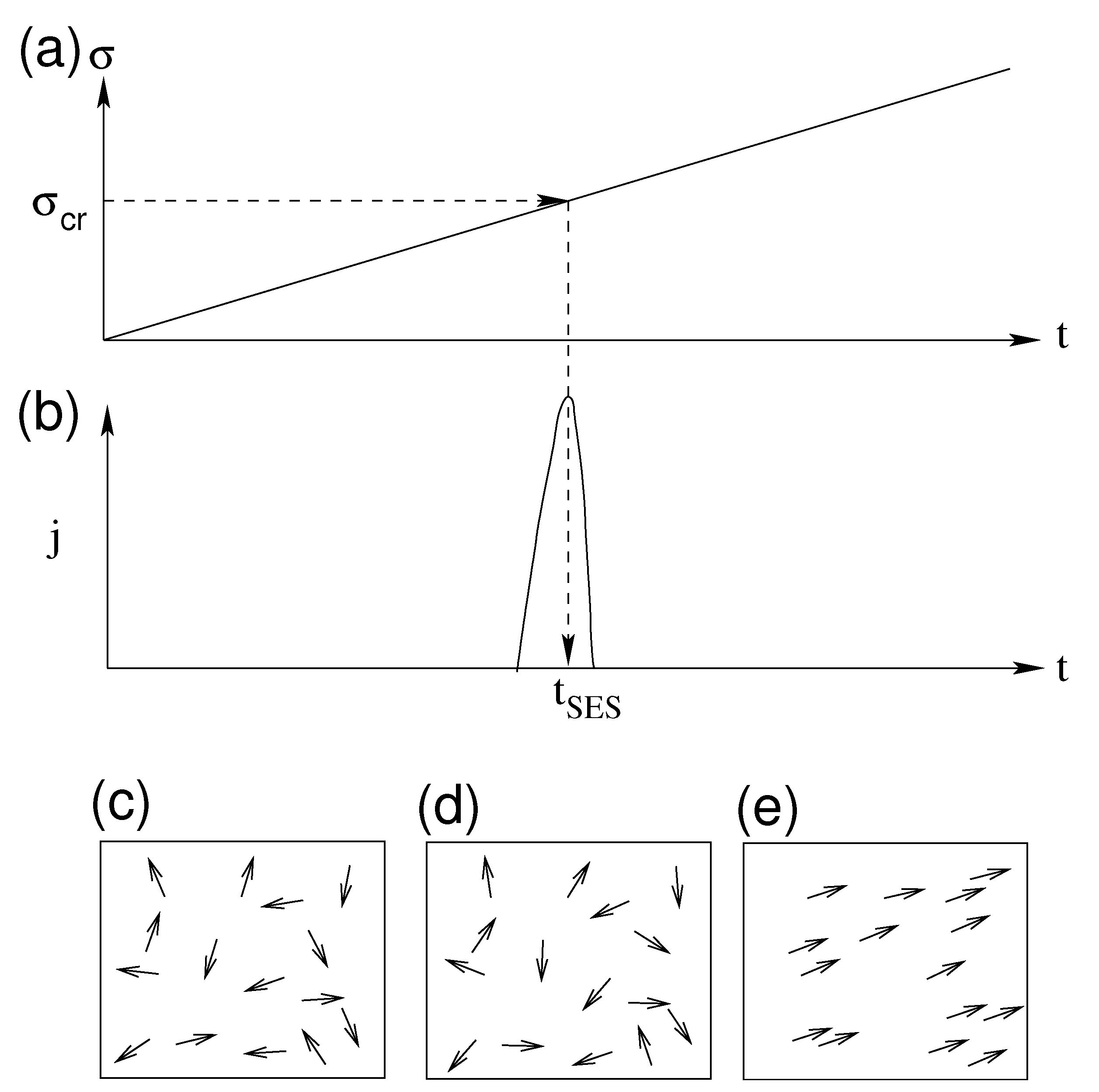
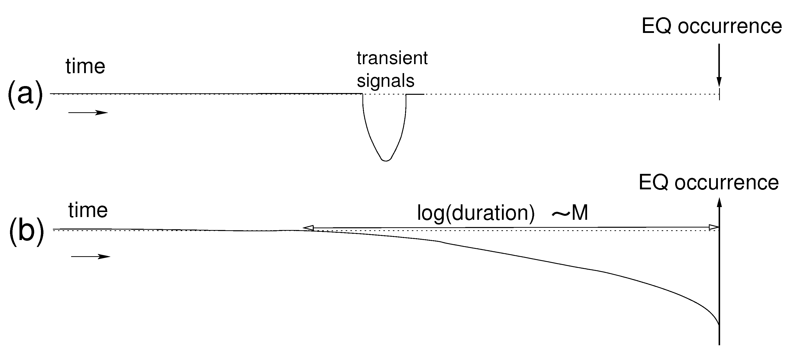
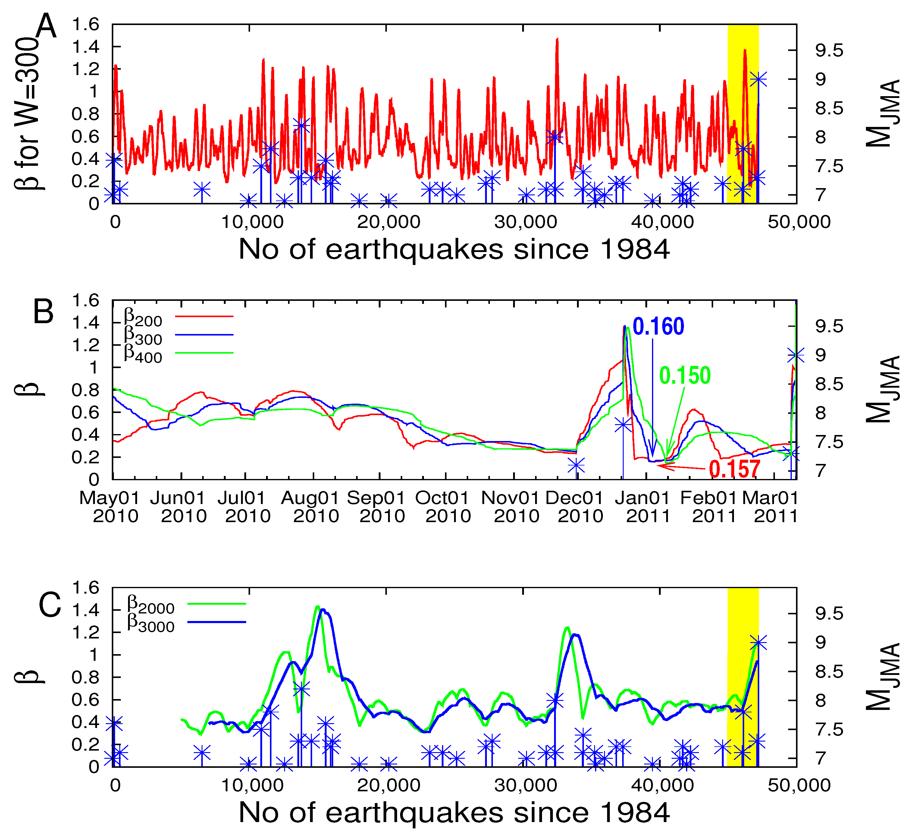
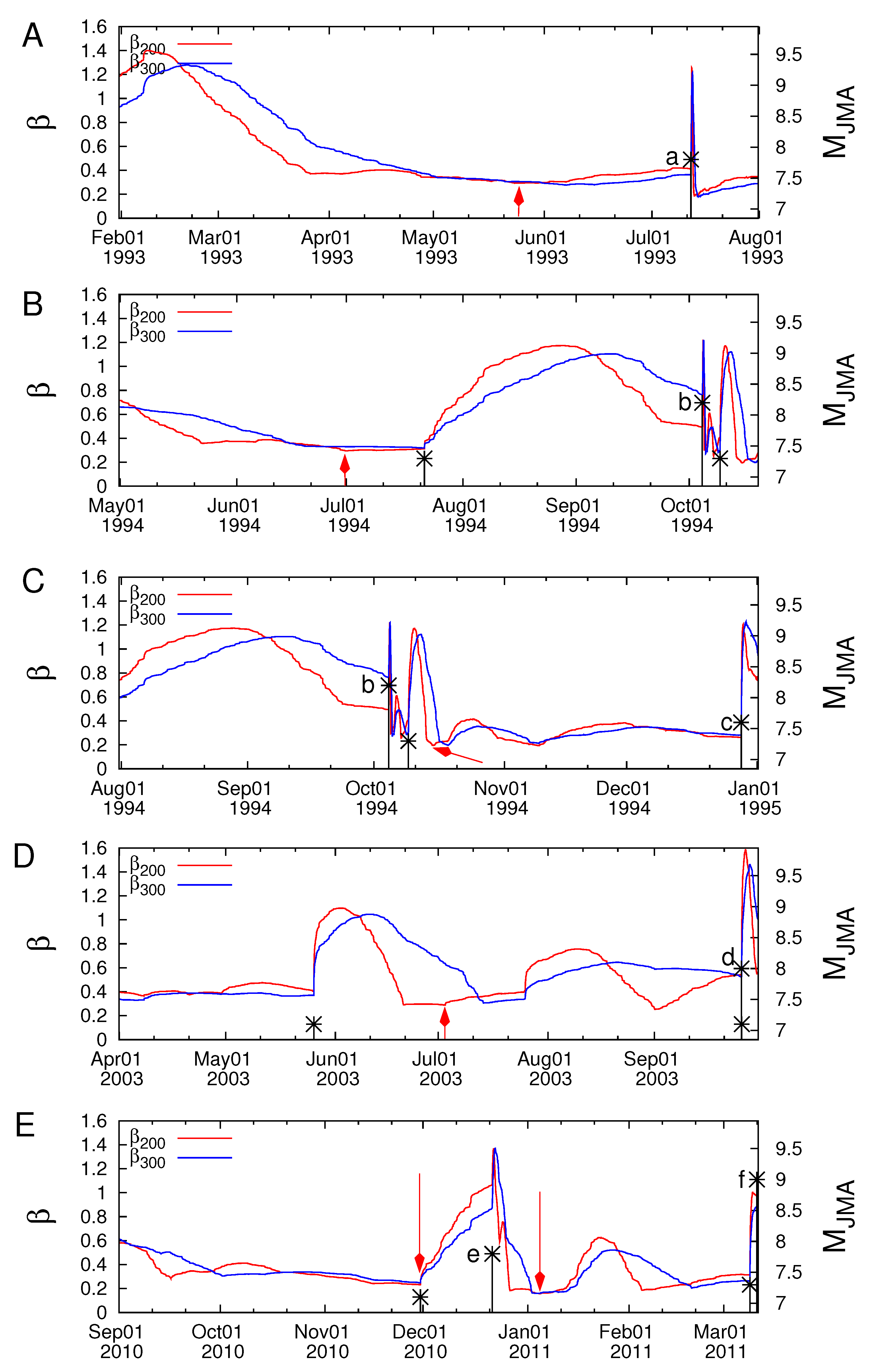
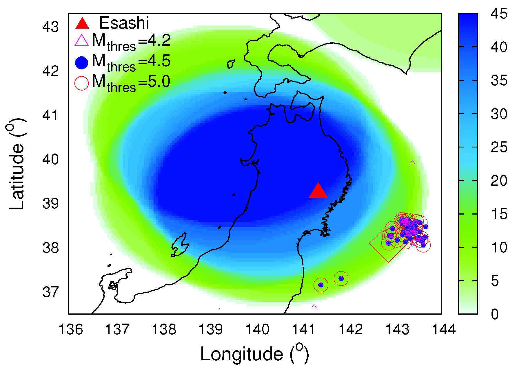
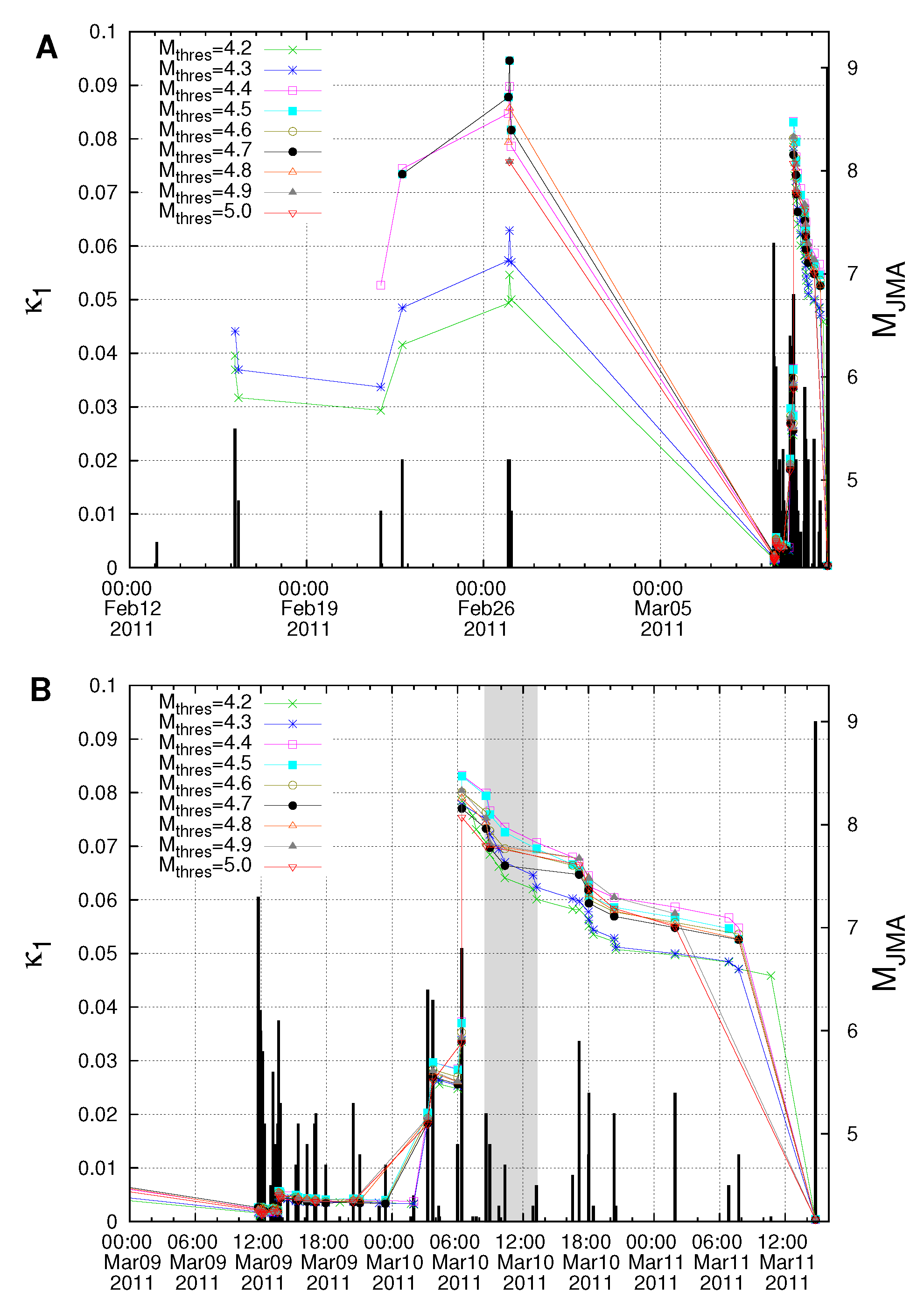
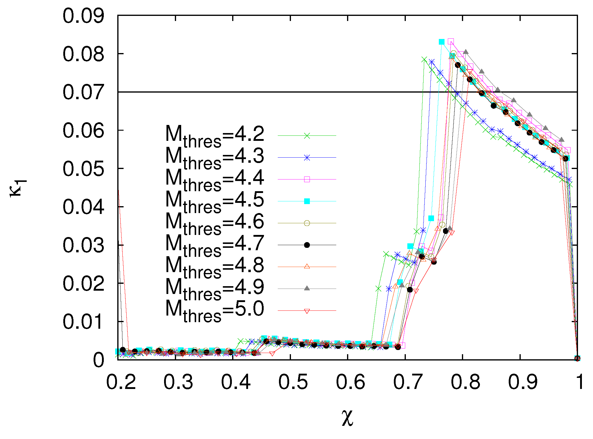
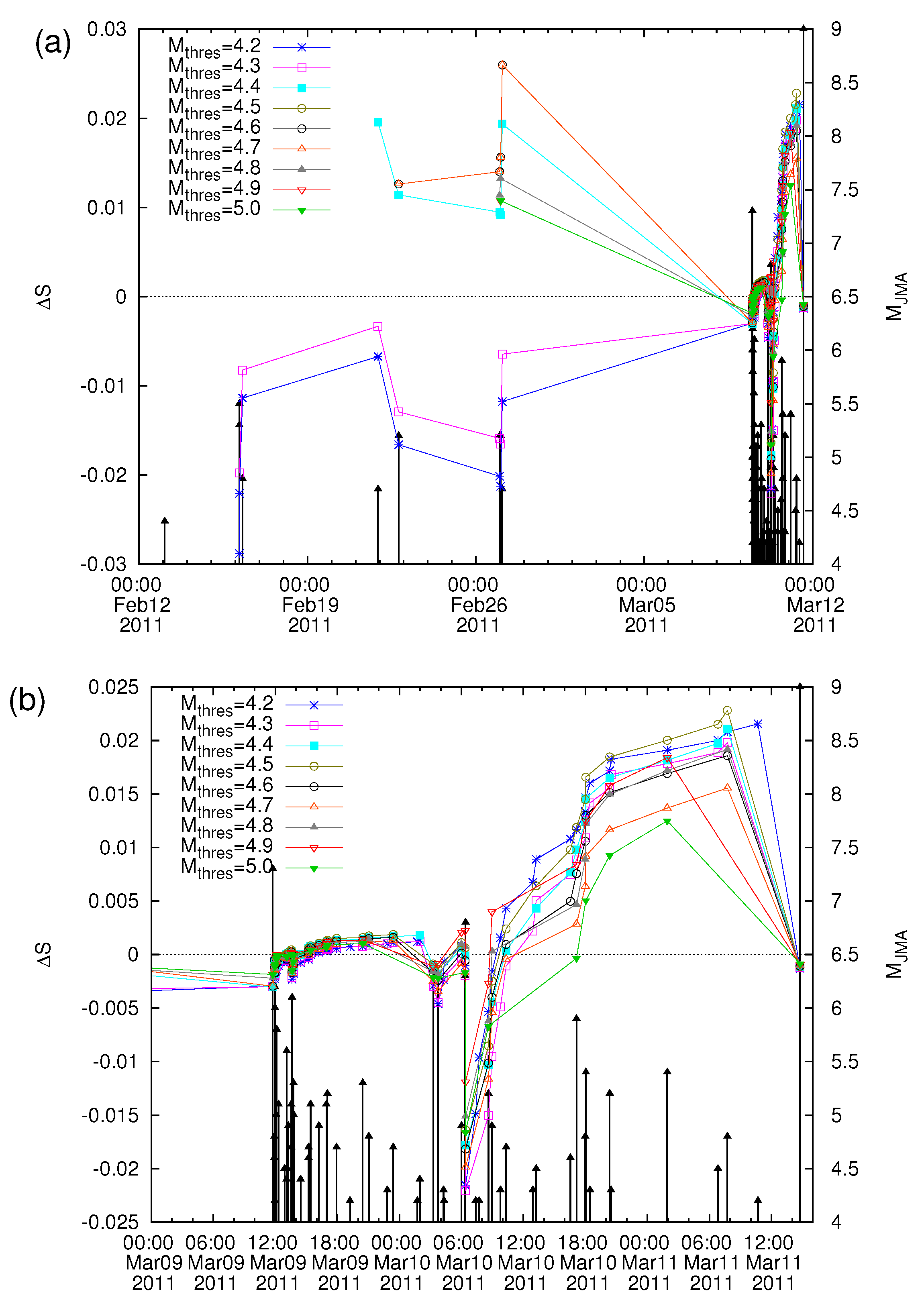
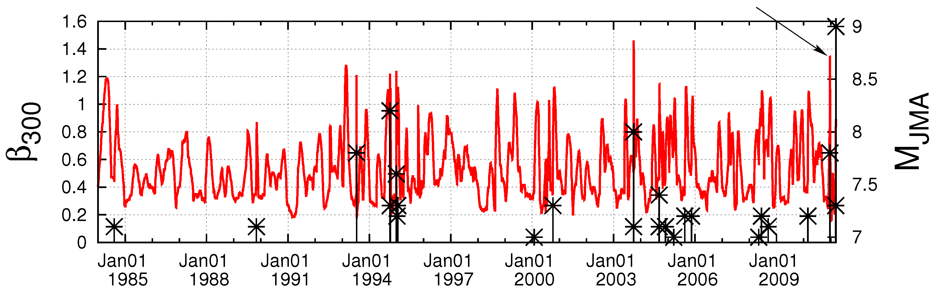
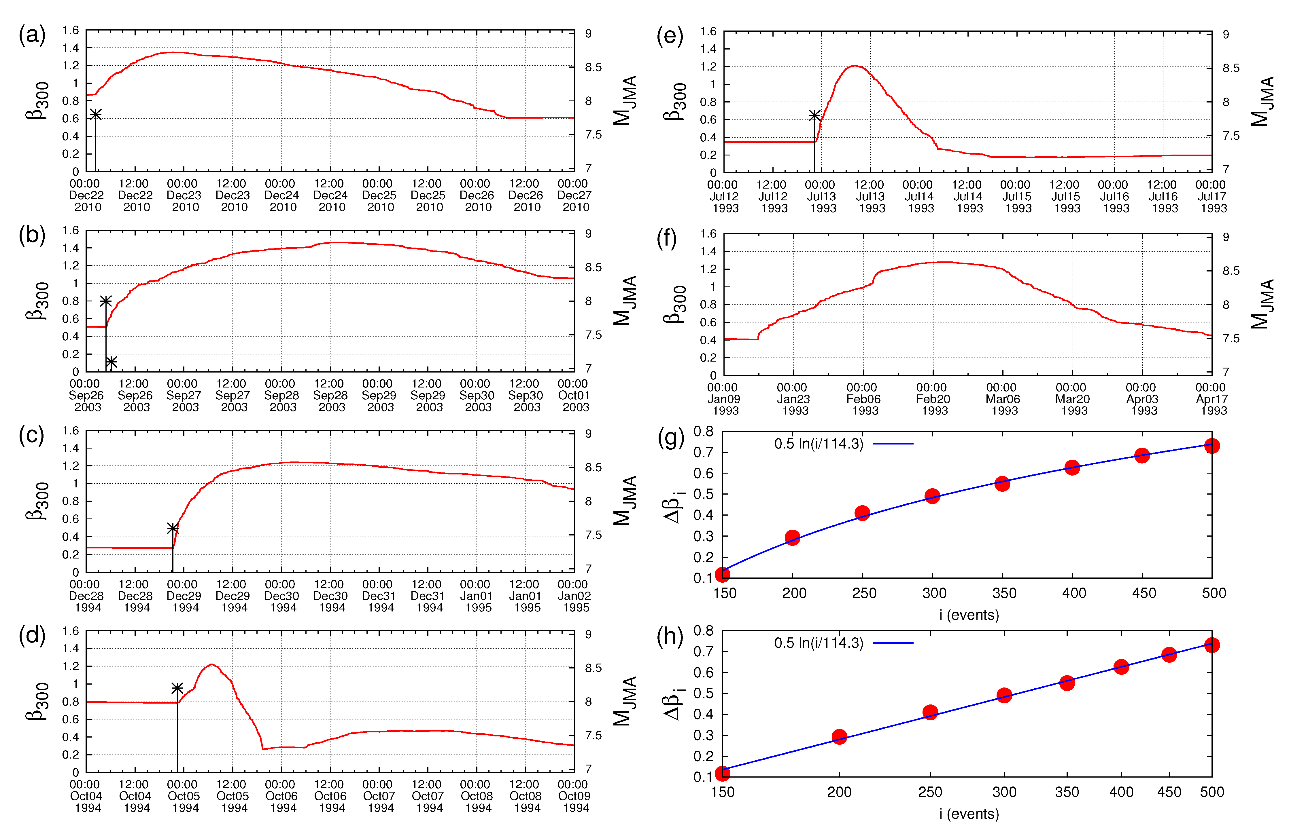
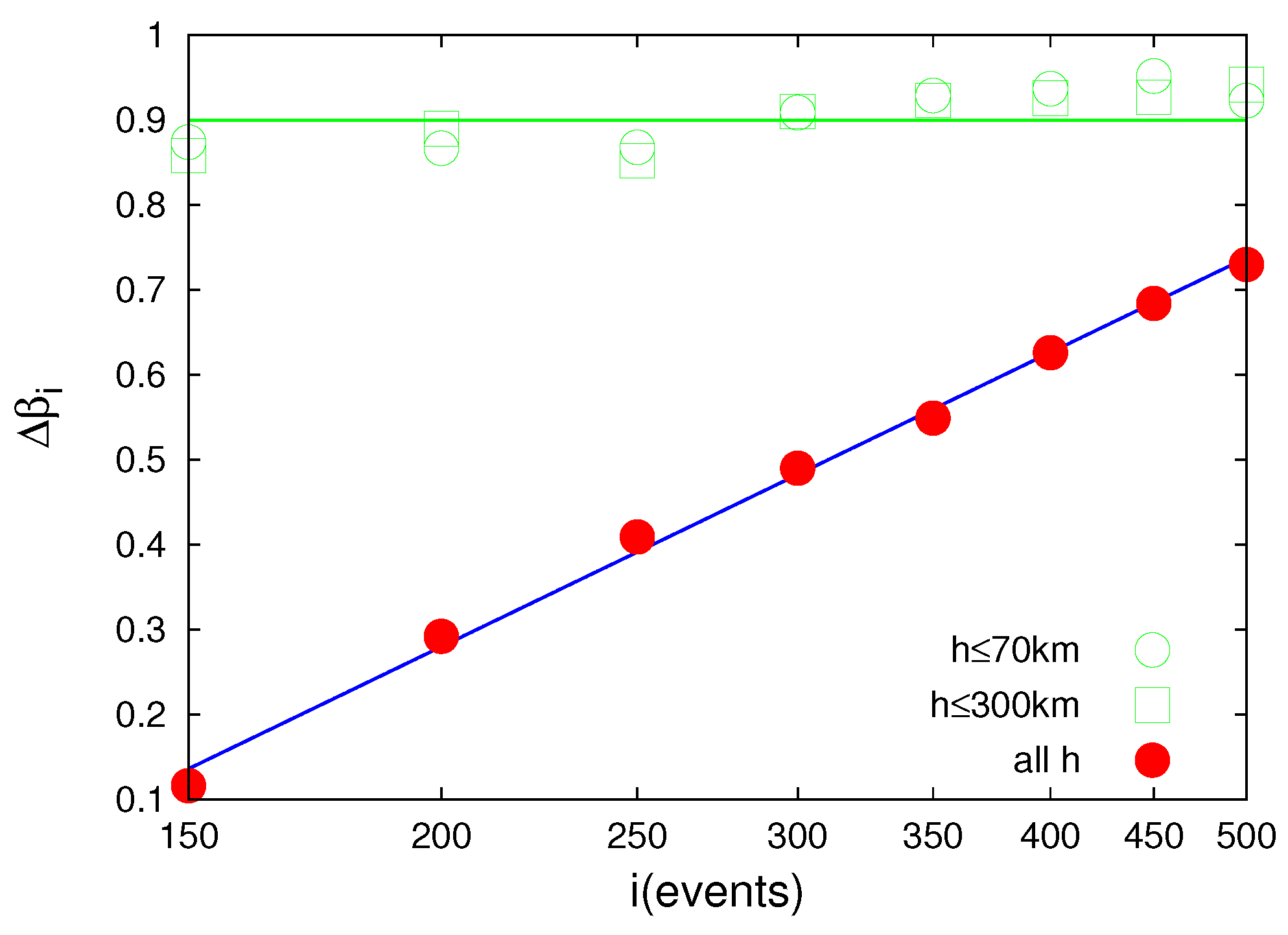
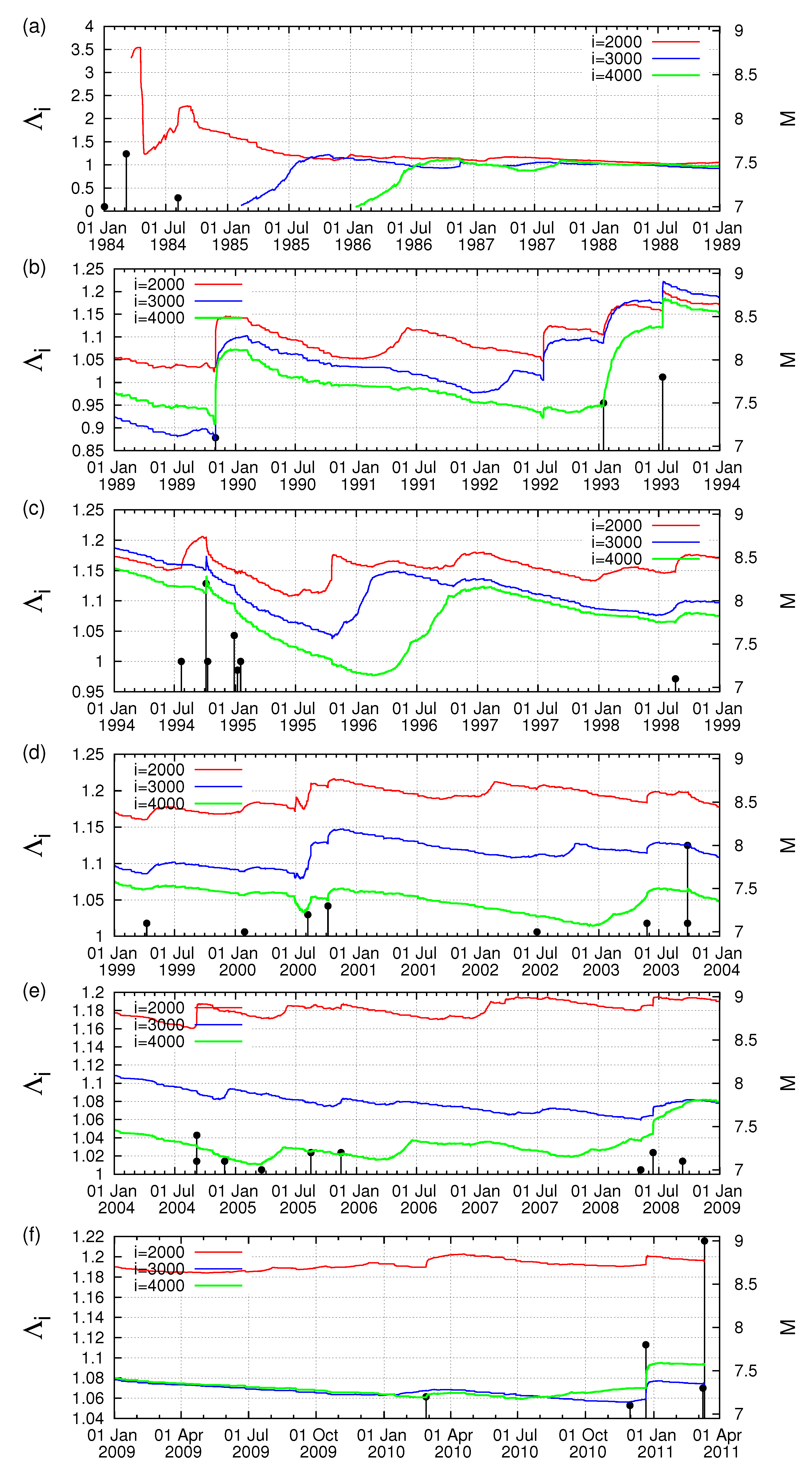
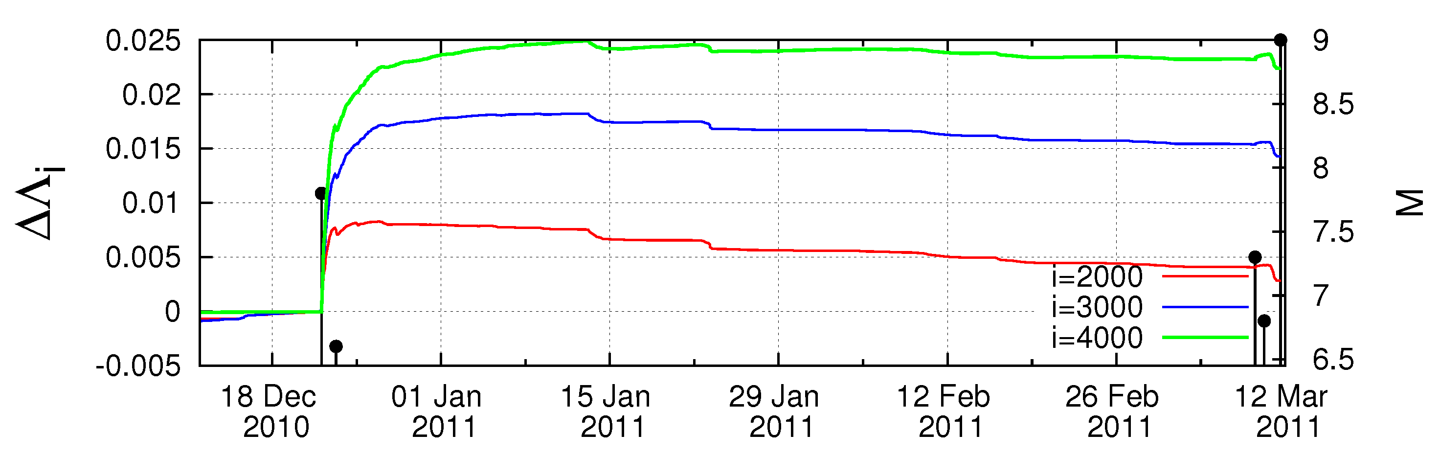
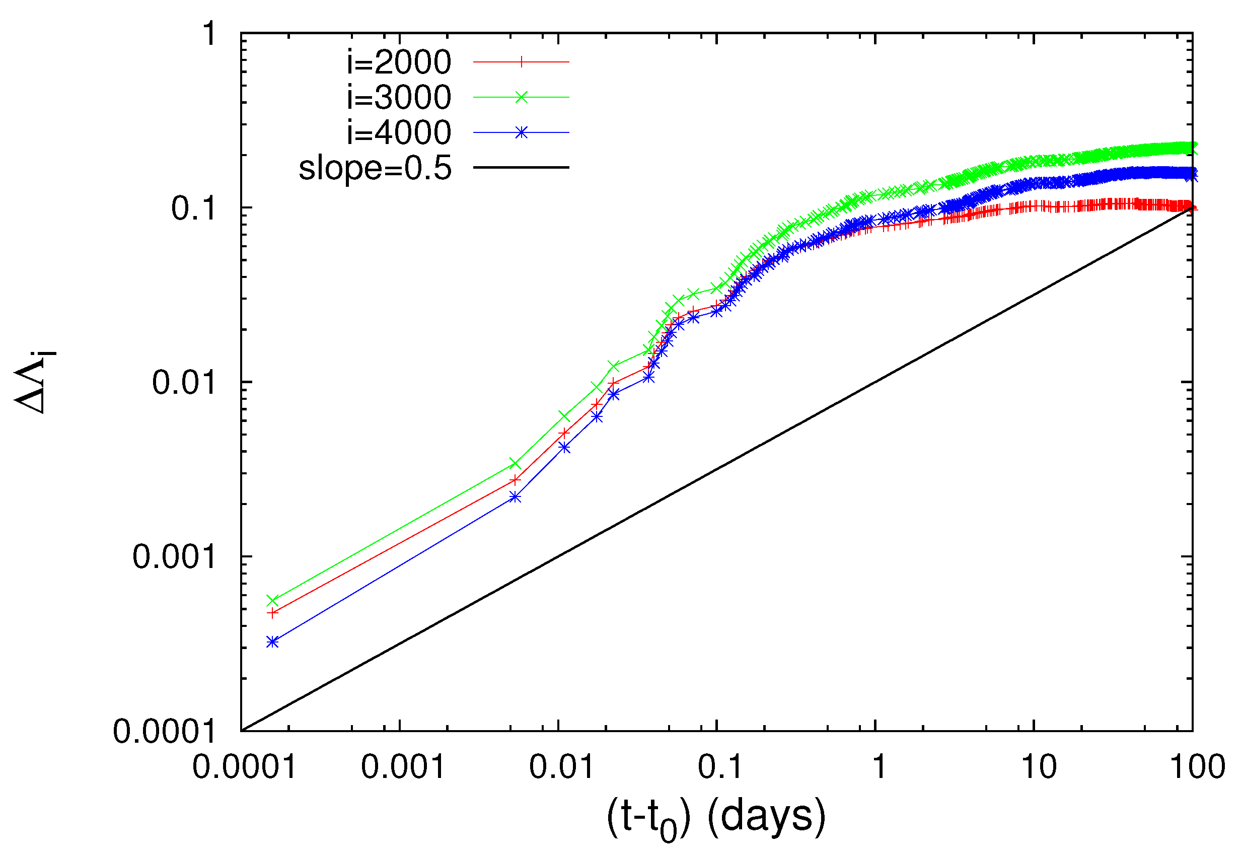
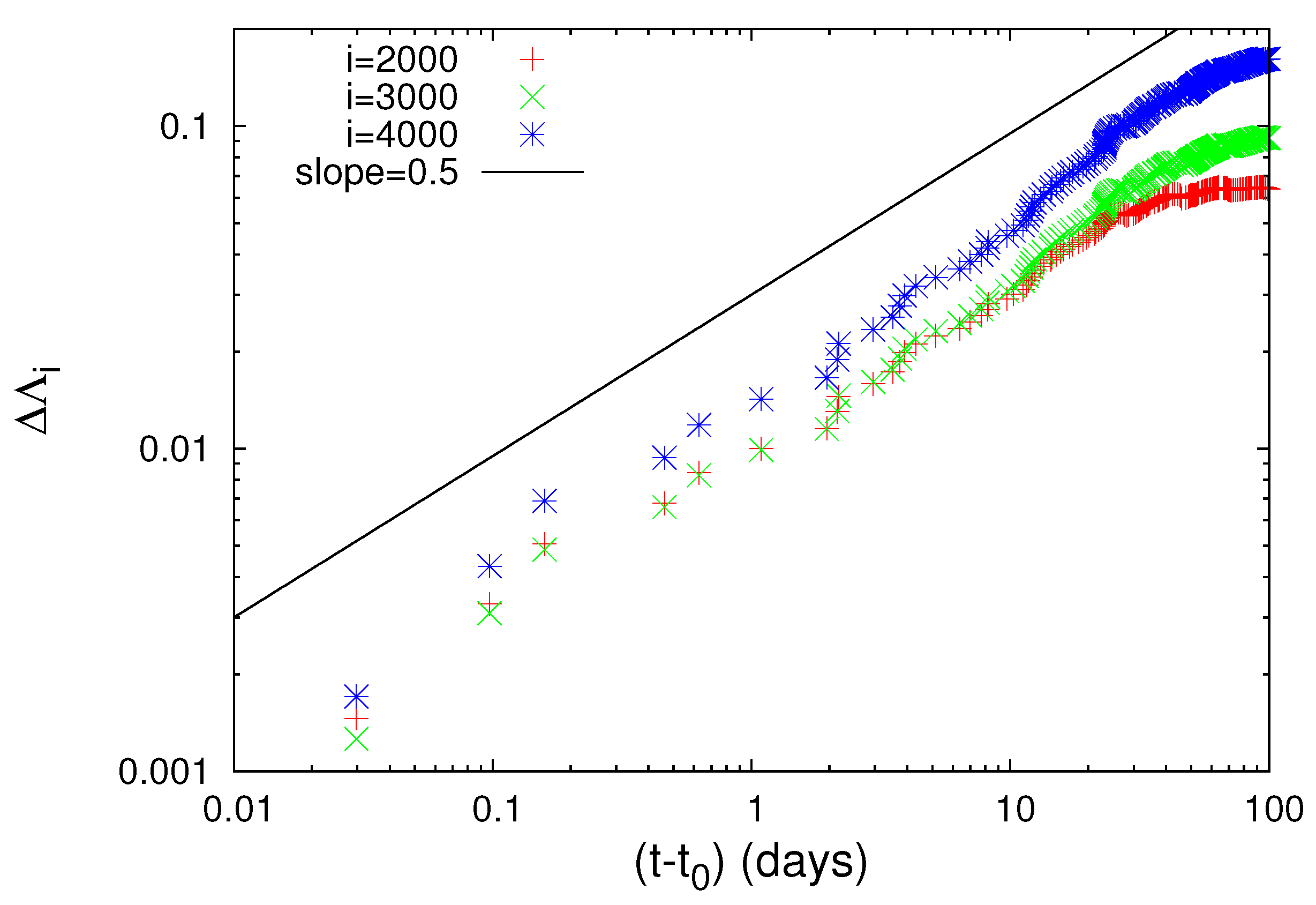
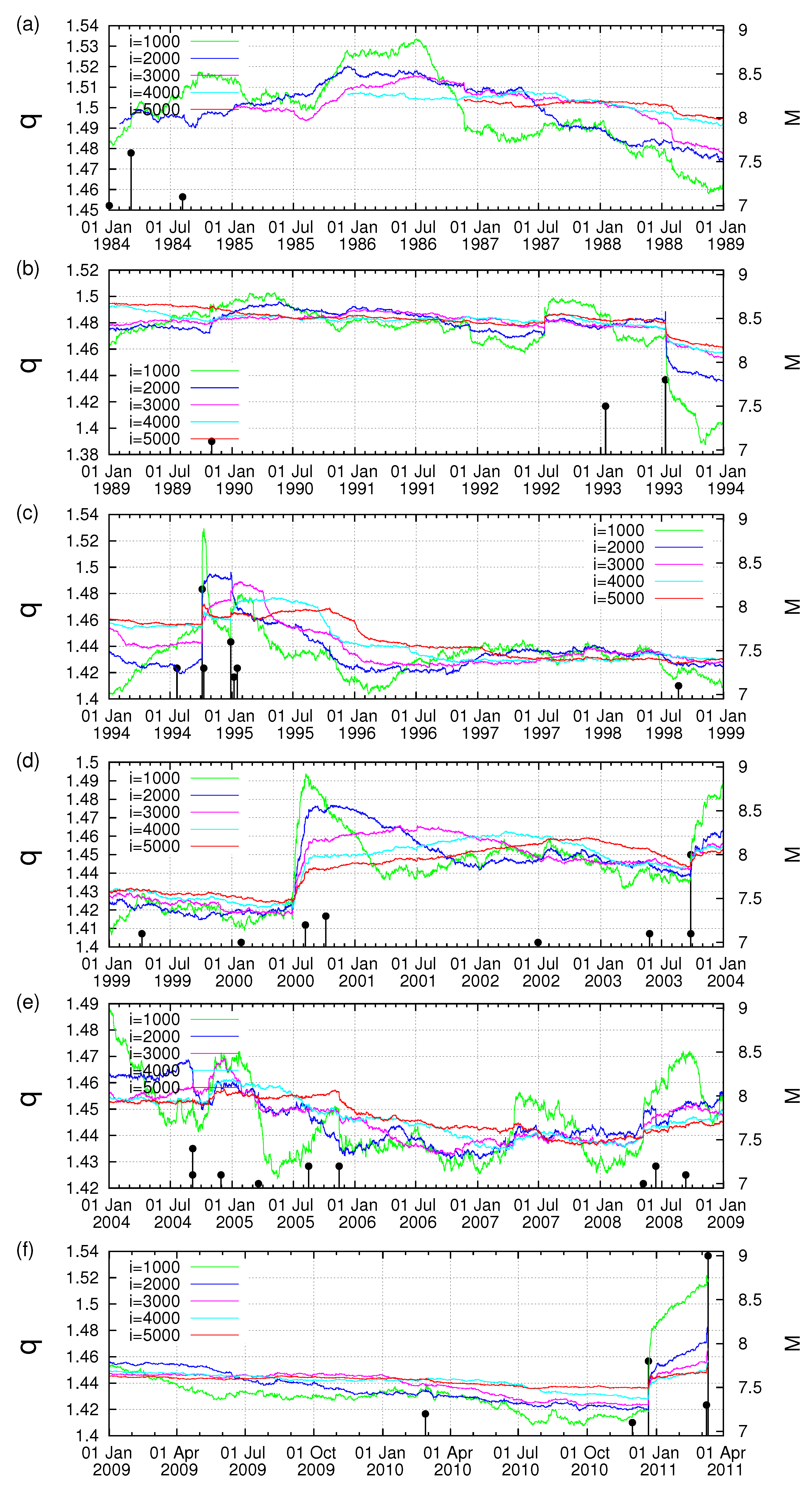
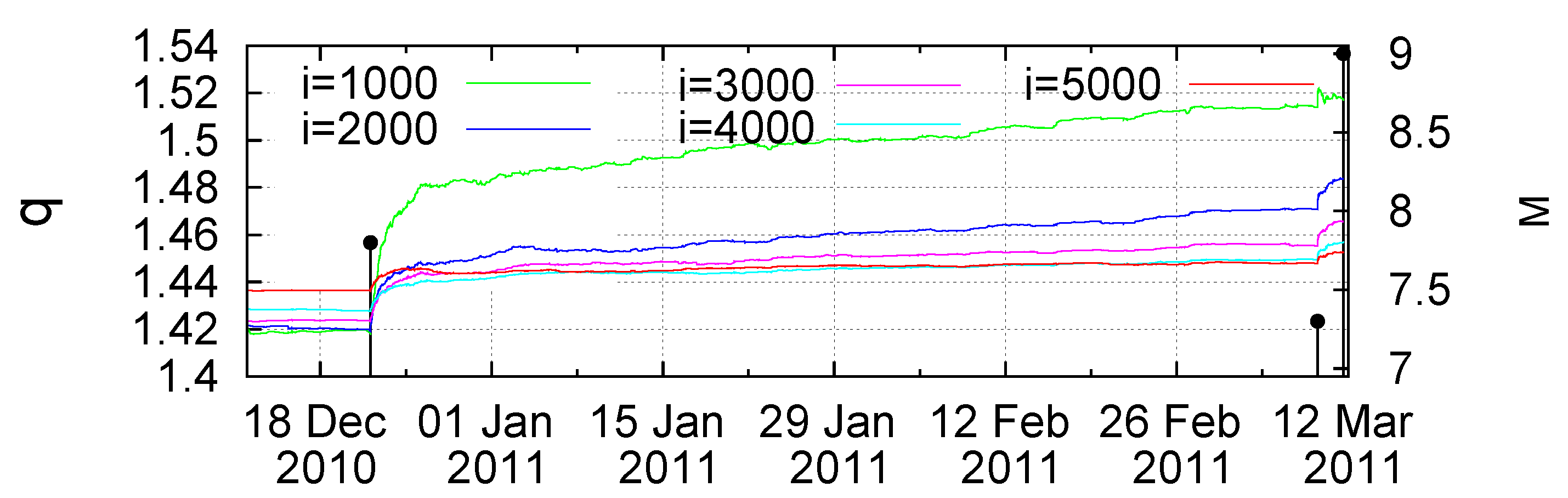
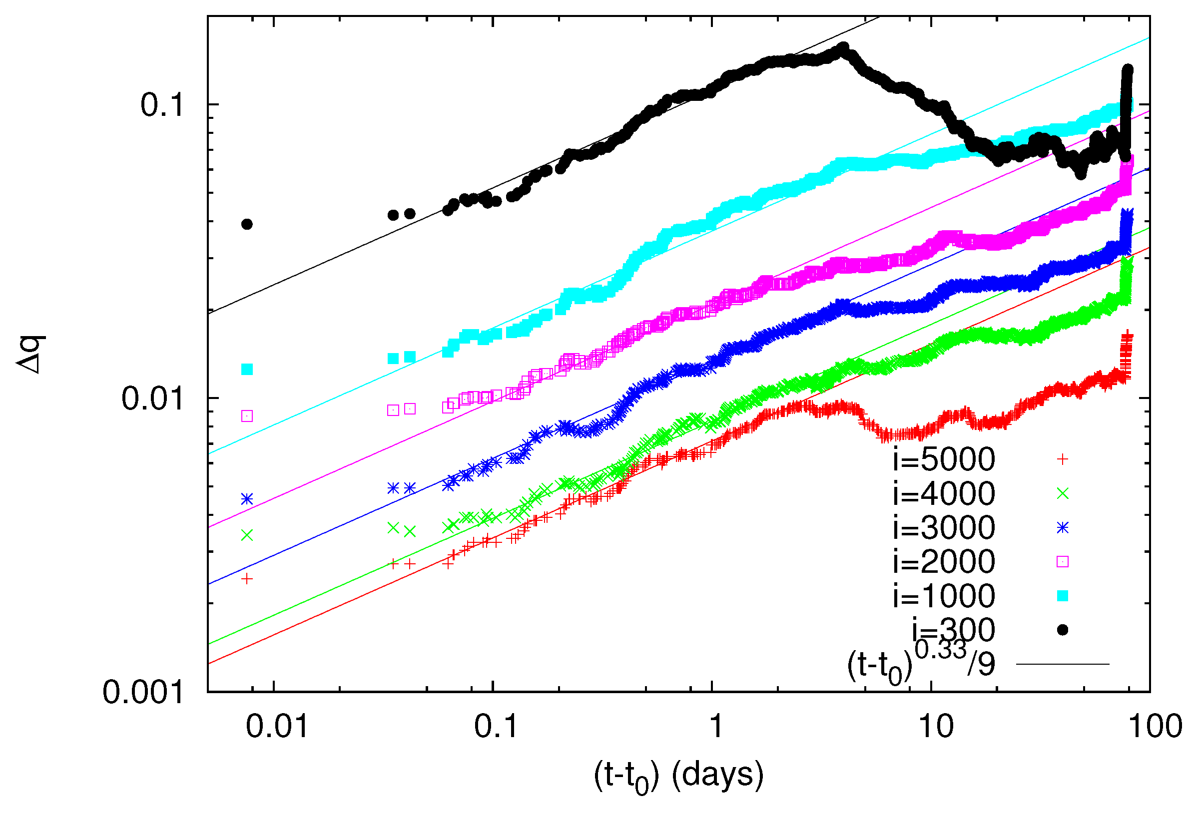
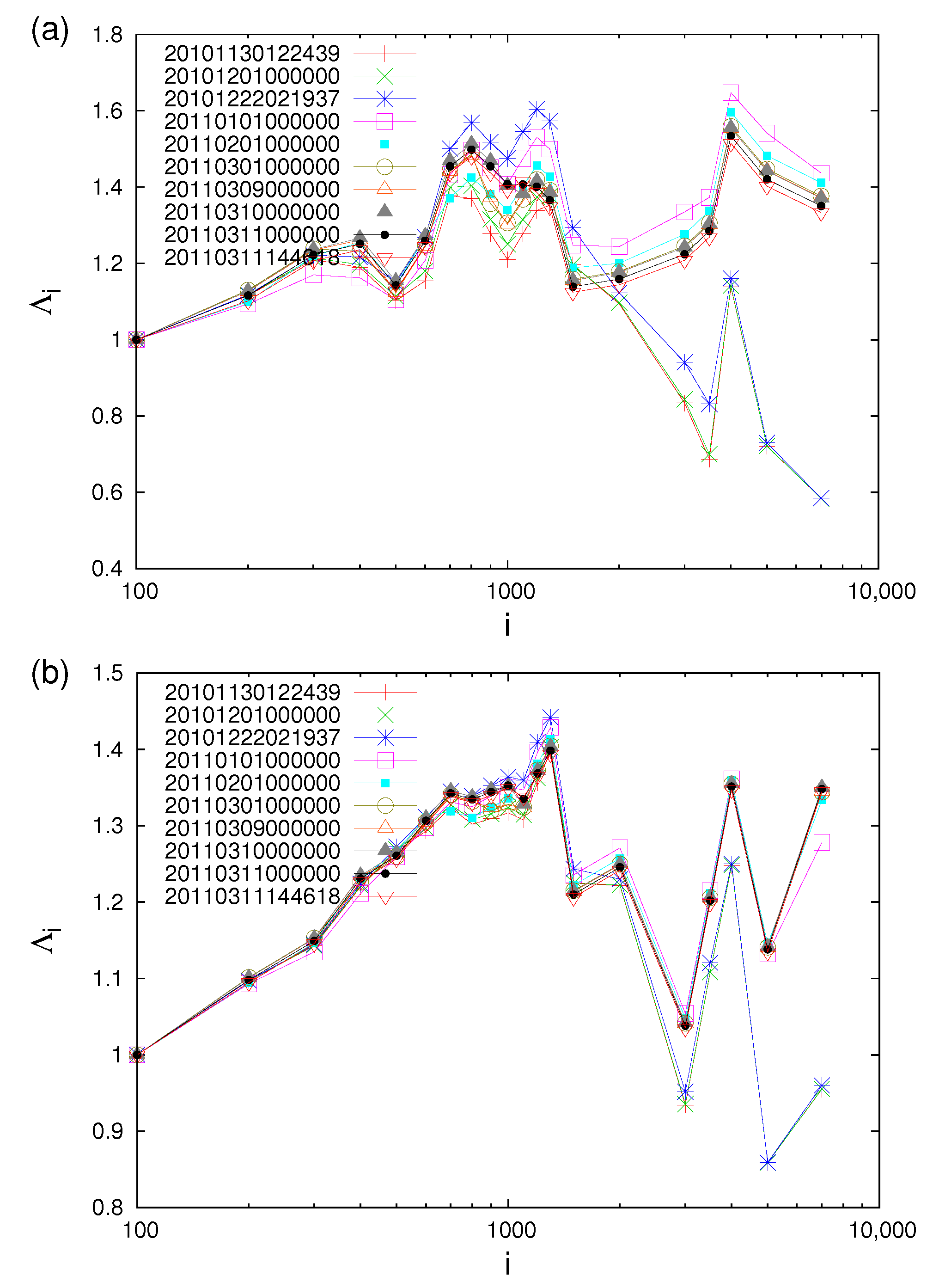
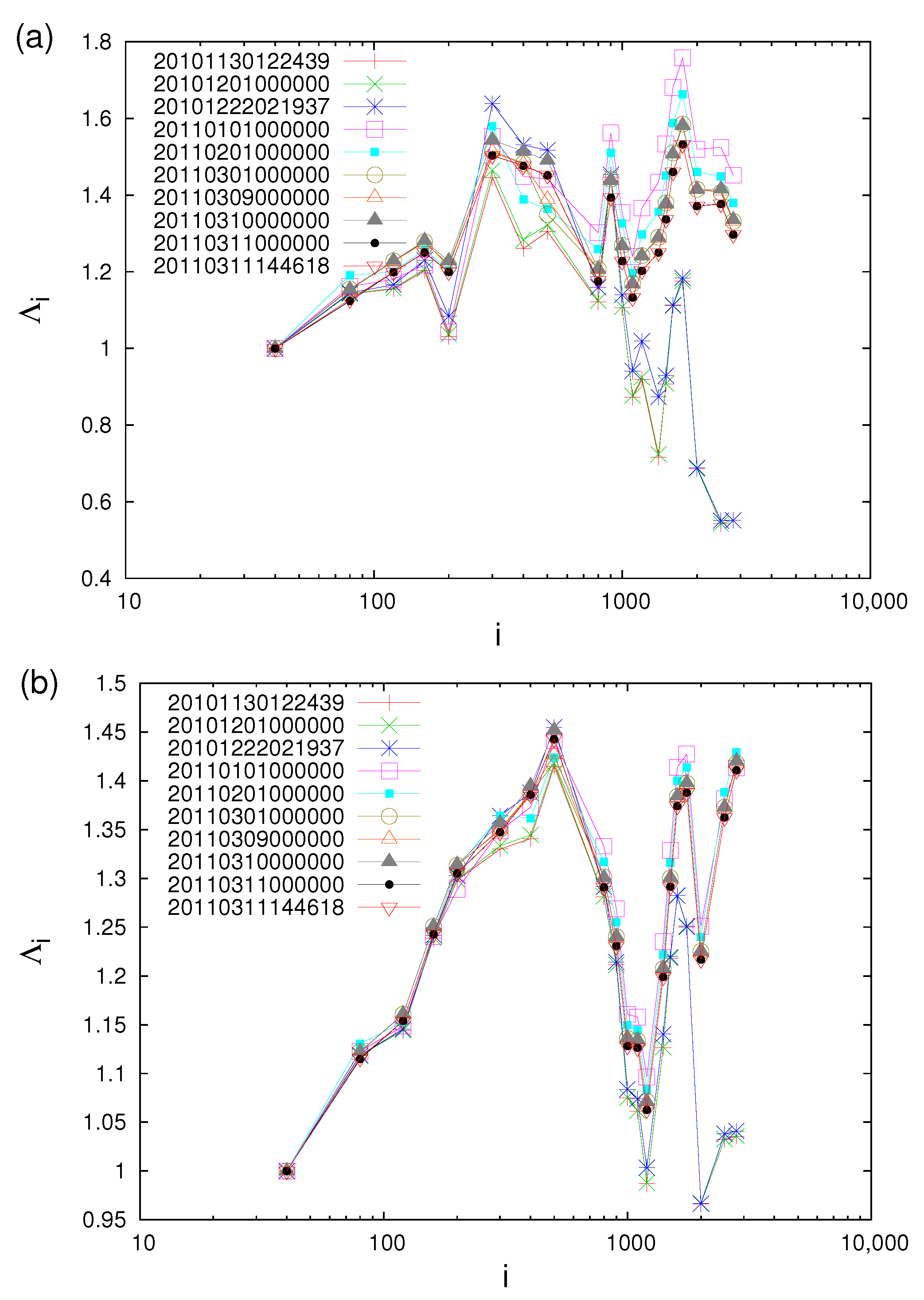
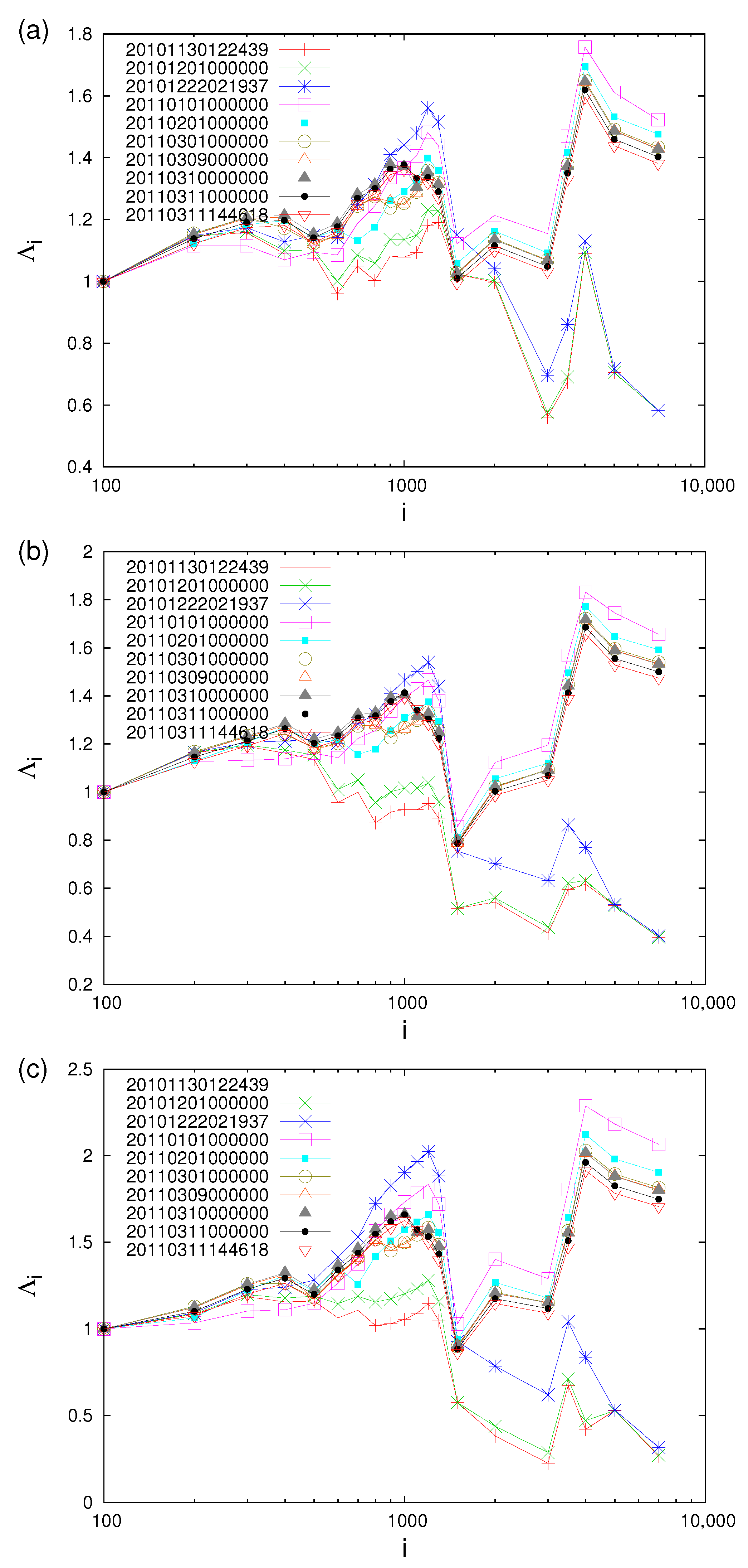
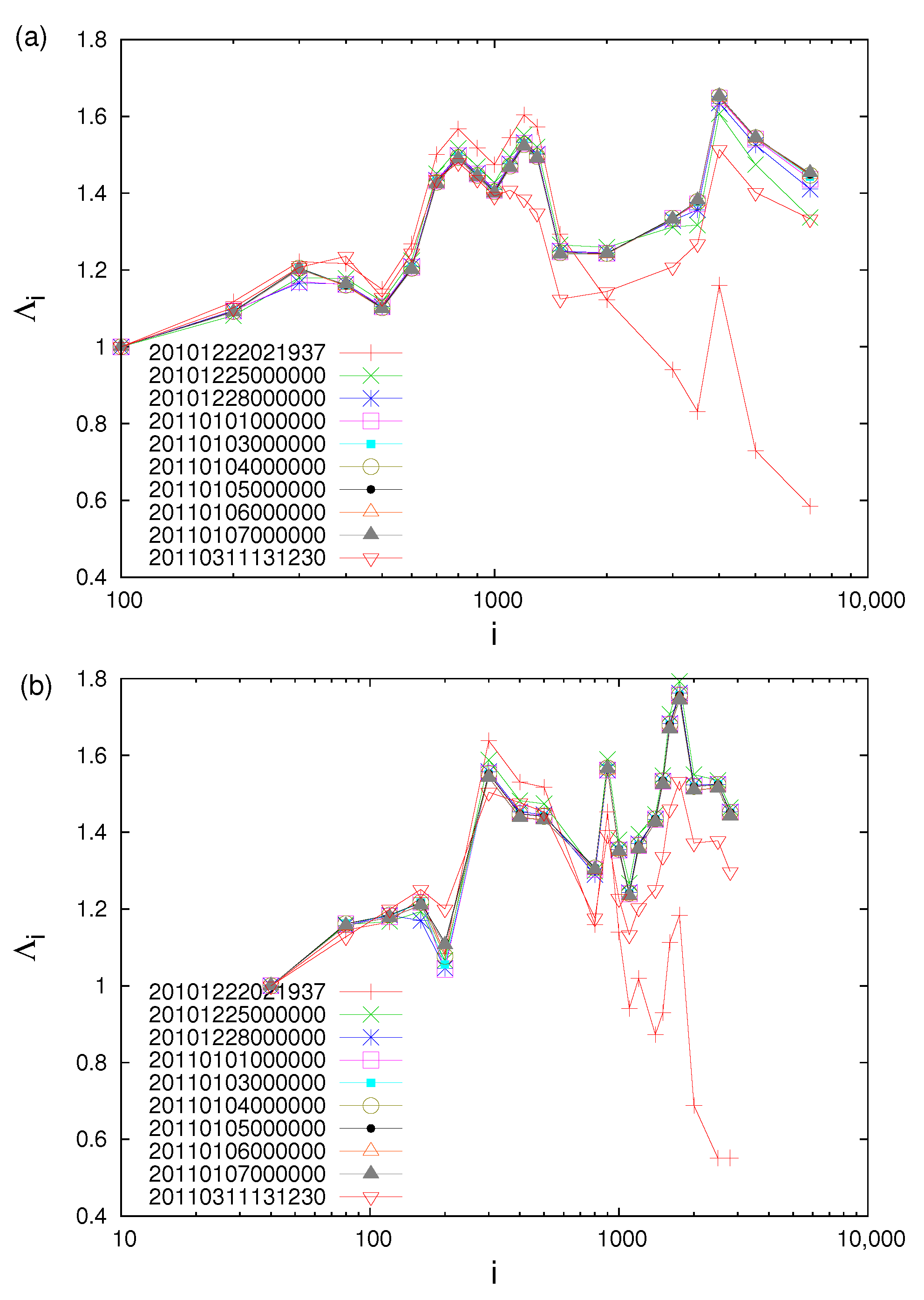
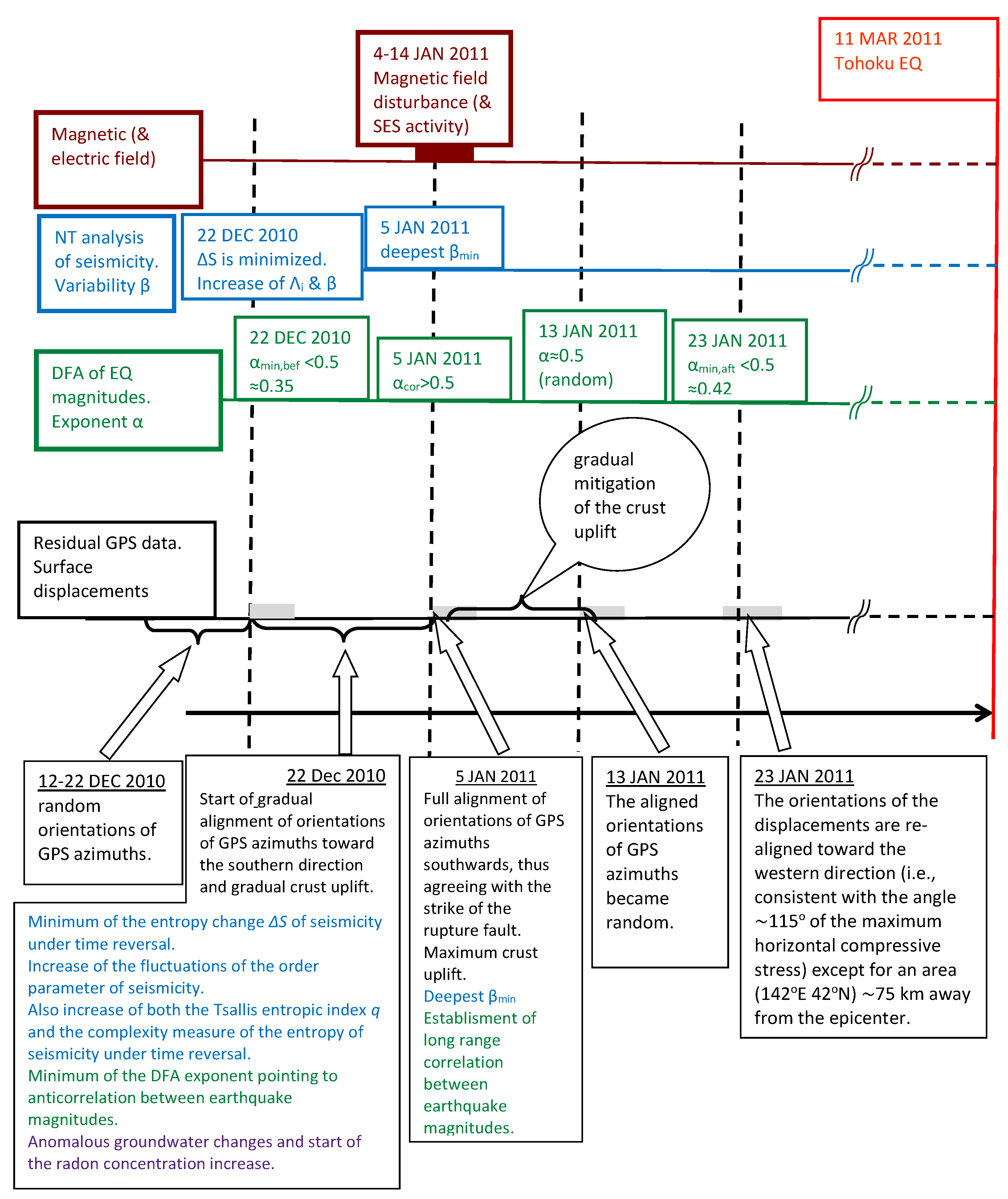
Table 1.
All EQs since 1 January 1984 until the M9 Tohoku EQ on 11 March 2011 in the larger area . Reproduced under permission from Ref. [44]. ©2014. American Geophysical Union. All Rights Reserved.
Table 1.
All EQs since 1 January 1984 until the M9 Tohoku EQ on 11 March 2011 in the larger area . Reproduced under permission from Ref. [44]. ©2014. American Geophysical Union. All Rights Reserved.
| Label | EQ Date | EQ Name | Lat. ( N) | Lon. ( E) | M |
|---|---|---|---|---|---|
| EQ1 | 12 July 1993 | Southwest-Off Hokkaido EQ | 42.78 | 139.18 | 7.8 |
| EQ2 1 | 4 October 1994 | East-Off Hokkaido EQ | 43.38 | 147.67 | 8.2 |
| EQ3 | 26 September 2003 | Off Tokachi EQ | 41.78 | 144.08 | 8.0 |
| EQ4 | 22 December 2010 | Near Chichi-jima EQ | 27.05 | 143.93 | 7.8 |
| EQ5 | 11 March 2011 | Tohoku EQ | 38.10 | 142.86 | 9.0 |
1 This EQ lies outside of the smaller area .
Table 2.
The values of , , and in the larger area investigated with sliding natural time windows of length 6 to W that preceded the EQs listed in Table 1. Hereafter, the value of is given when appears and is the minimum of the DFA exponent up to three-and-a-half months (105 days) before . Reproduced under permission from Ref. [44]. ©2014. American Geophysical Union. All Rights Reserved.
| Label | |||||||
|---|---|---|---|---|---|---|---|
| EQ1 | 0.292(19930523) 1 | 0.266(19930602) | 0.270(19930607) | 0.92 | 0.397(19930327) | 0.515(19930602) | 0.469(19930613) |
| EQ2 | 0.294(19940630) | 0.274(19940722) | 0.312(19940722) | 1.06 | 0.451(19940627) | 0.557(19940722) | 0.476(19940724) |
| EQ3 | 0.289(20030703) 2 | 0.273(20030703) | 0.307(20030714) | 1.06 | 0.356(20030325) | 0.553(20030703) | 0.384(20030925) 3 |
| EQ4 | 0.233(20101130) | 0.221(20101130) | 0.242(20101130) | 1.04 | 0.467(20101116) | 0.501(20101130) | 0.385(20101201) |
| EQ5 | 0.156(20110105) | 0.160(20110108) | 0.154(20110105) | 0.99 | 0.348(20101222) | 0.524(20110108) | 0.422(20110123) |
1 A comparable (within ± 0.0005) value = 0.293 is also found on 24 May 1993. 2 The same (within ± 0.0005)
value = 0.289 is also found on 21 June 2003. 3 The date of the M8 EQ is either 25 or 26 September 2003
depending on the use of LT or UT, respectively. Here, we use LT. This value of a is observed 15.5 h before the
mainshock.
Table 3.
The values of , , and in the smaller area investigated with sliding natural time windows of length 6 to W that preceded EQs. Reproduced under permission from Ref. [44]. ©2014. American Geophysical Union. All Rights Reserved.
Table 3.
The values of , , and in the smaller area investigated with sliding natural time windows of length 6 to W that preceded EQs. Reproduced under permission from Ref. [44]. ©2014. American Geophysical Union. All Rights Reserved.
| Label | |||||||
|---|---|---|---|---|---|---|---|
| EQ1 | 0.288(19930526) | 0.264(19930607) | 0.278(19930607) | 0.97 | 0.374(19930319) | 0.557(19930607) | 0.473(19930617) |
| EQ3 1 | 0.293(20030624) | 0.311(20030709) | 0.309(20030718) | 1.06 | 0.374(20030408) | 0.570(20030709) | 0.434(20030925) 2 |
| EQ4 | 0.228(20101130) | 0.233(20101130) | 0.250(20101130) | 1.09 | 0.467(20101122) | 0.516(20101130) | 0.408(20101209) |
| EQ5 | 0.156(20110105) | 0.160(20110108) | 0.154(20110105) | 0.99 | 0.354(20101222) | 0.522(20110108) | 0.439(20110117) |
1 The epicenter of EQ2—not included here—lies outside of the smaller area. 2 The date of the M8 EQ is either 25
or 26 September 2003 depending on the use of LT or UT, respectively. Here, we use LT. This value of α is observed
24.5 h before the mainshock.
Publisher’s Note: MDPI stays neutral with regard to jurisdictional claims in published maps and institutional affiliations. |
© 2022 by the authors. Licensee MDPI, Basel, Switzerland. This article is an open access article distributed under the terms and conditions of the Creative Commons Attribution (CC BY) license (https://creativecommons.org/licenses/by/4.0/).
Share and Cite
MDPI and ACS Style
Varotsos, P.A.; Sarlis, N.V.; Skordas, E.S. Order Parameter and Entropy of Seismicity in Natural Time before Major Earthquakes: Recent Results. Geosciences 2022, 12, 225. https://0-doi-org.brum.beds.ac.uk/10.3390/geosciences12060225
AMA Style
Varotsos PA, Sarlis NV, Skordas ES. Order Parameter and Entropy of Seismicity in Natural Time before Major Earthquakes: Recent Results. Geosciences. 2022; 12(6):225. https://0-doi-org.brum.beds.ac.uk/10.3390/geosciences12060225
Chicago/Turabian StyleVarotsos, Panayiotis A., Nicholas V. Sarlis, and Efthimios S. Skordas. 2022. "Order Parameter and Entropy of Seismicity in Natural Time before Major Earthquakes: Recent Results" Geosciences 12, no. 6: 225. https://0-doi-org.brum.beds.ac.uk/10.3390/geosciences12060225
Note that from the first issue of 2016, this journal uses article numbers instead of page numbers. See further details here.