
GRACE Accelerometers Sensitive to Ionosphere Plasma Waves: Similarities between Twangs and Whistlers

School of Engineering and Design, Technical University of Munich, 80333 Munich, Germany
Geosciences 2022, 12(6), 228; https://0-doi-org.brum.beds.ac.uk/10.3390/geosciences12060228
Submission received: 14 April 2022
/
Revised: 18 May 2022
/
Accepted: 20 May 2022
/
Published: 27 May 2022
Abstract
:Electrostatic space accelerometers are high-precision instruments used in gravity and magnetic fields and in fundamental physics missions. From their first use in space, these instruments show disturbances around the read-out frequency. In recent missions like Swarm and GRACE-FO, these instruments are seriously compromised. Their capability cannot be fully exploited or, in the worst case, not used for science data processing at all. We currently neither understand the mechanism nor the cause of the disturbance. For that reason, every correlation, direct or indirect, between signatures in the accelerometer data and other phenomena in the satellite environment is very important to study. In the GRACE mission, some of the disturbances relate to onboard current switching processes, such as switching of heater and torquer currents. In this paper, we examine the phenomena called twangs. The shape of these disturbances is responsible for their name, because they look like a decaying tone. Some of these twangs seem to relate to changing currents, too. They occur when sunlight hits surfaces of the satellite. This can cause the discharging of satellite parts. Here, we focus on special twangs, which we call cloud-related twangs, as recent investigations related them to cloud coverage. How can clouds in the troposphere influence a satellite, orbiting in the ionosphere? We investigated the troposphere–ionosphere coupling and found that the only coupling which can be responsible for disturbances on satellites and which may affect the accelerometers, are electromagnetic waves traveling in the so-called whistler mode at frequencies in the very-low-frequency (VLF) domain. This special propagation mode is a coupled electromagnetic and electrostatic mode. There, the electric field vector has a component in the direction of propagation due to the interaction with ions and the magnetic field in the ionosphere and magnetosphere. This led us to investigate the similarities between whistlers and twangs. The hypothesis that they are related is very important in our further understanding of disturbances on satellite instruments sensible to electromagnetic pulses in the range of very low frequencies and below.
1. Introduction
Electrostatic space accelerometers are widely used instruments on satellite missions [1]. They sense the nongravitational accelerations on low-orbiting satellites in gravity field missions [2], such as the Challenging Minisatellite Payload (CHAMP), the Gravity Recovery and Climate Experiment (GRACE), and GRACE follow-on (GRACE-FO), as well as in magnetic field missions such as Swarm [3]. Six of these instruments form the gravity gradiometer in the GOCE mission [4]. Fundamental physics missions use them to detect a violation of the equivalence principle (MICROSCOPE) [5]. The inertial sensors on gravitational waves mission LISA work slightly different but are comparable [6]. LISA Pathfinder was the test mission for LISA, and it showed that the sensor achieved the necessary performance for the LISA mission [7].
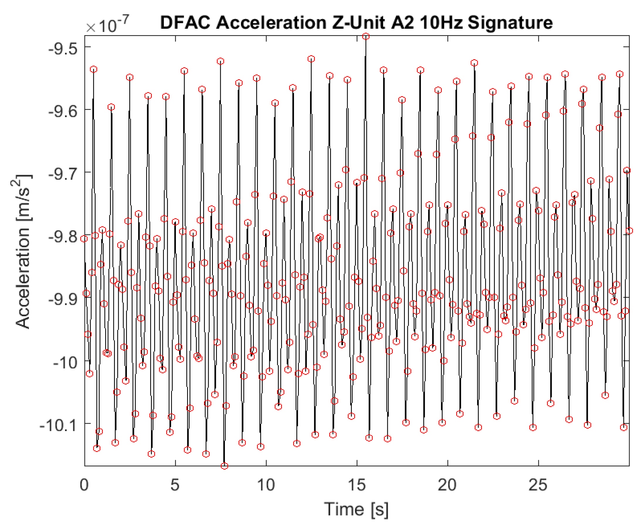
All these missions were profoundly successful, but their accelerometers had signals in common which did not relate to surface forces acting on the satellite. On most missions, the frequency of the disturbances is around the read-out frequency of the accelerometers and, hence, far away from the measurement band of the data analysis. The disturbances do not harm the mission objectives in these cases. Figure 1 shows an example for the 10 Hz read-out of the GOCE mission. For a discussion of signatures on the CHAMP mission, compare the studies by Gruenwald et al. [8,9]. The best-studied instruments have been on the GRACE mission. Here, different types of sources produce the disturbances.
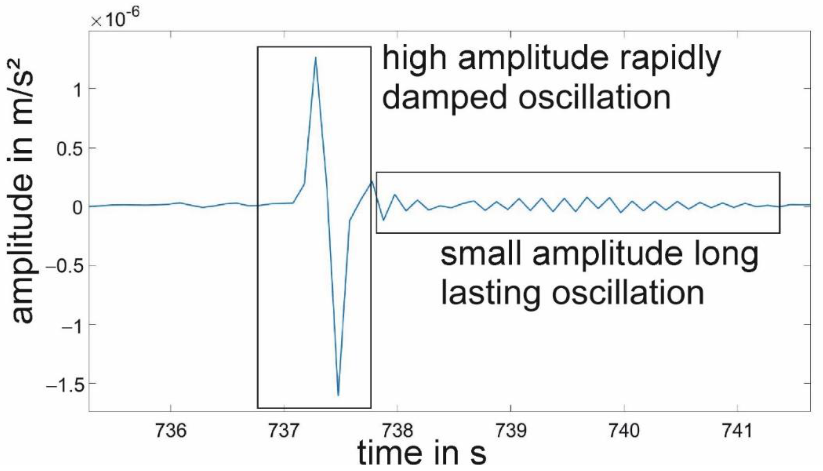
Flury et al. [10] related some spikes to switching of currents in the heaters, while Peterseim et al. [11] related others to current switching on torquers. The disturbances with the greatest amplitude are so-called twangs. They reach amplitudes of three or more orders of magnitude of the resolution of the instruments. Figure 2 is an example of such a disturbance. The disturbances got the name ‘twang’ due to the long-lasting oscillation accompanying the high-amplitude spikes.
Peterseim [12] proposed that twangs can have various origins: discharging events due to sunlight hitting parts of the satellite structure (charging explained, e.g., in [13]); discharging of the Teflon foil mounted on the nadir side of the satellite as Teflon becomes photoconductive; others related to the switching of the battery from charging to discharging and vice versa. Most origins seem related to the troposphere, as a relation with cloud coverage was proposed.
All the disturbances have a remarkable fact in common: the influence on the axes of the accelerometer is different and varies with the position of the heater. This allows two possible explanations: the signatures are real accelerations or shifts in the center of mass; alternatively, they are of electrostatic and electromagnetic origin and disturb the sensor head.
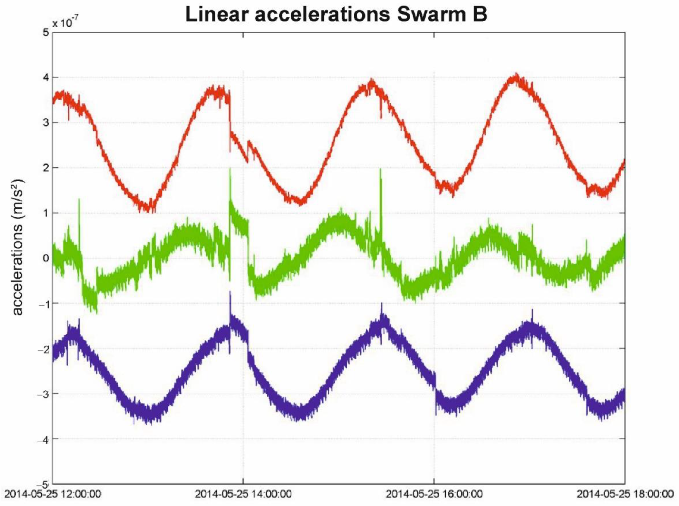
Much more dramatic is the situation with the accelerometers on GRACE-FO and Swarm. Figure 3 shows a timeseries of the accelerometer on Swarm B. This accelerometer not only shows spikes, but also sudden bias changes. Siemes et al. [14] discussed two hypotheses for the occurrence of these steps not related to failure of the instrument: thermomechanical stress on the sensor head or radiation effects on the electrical components. The correction and calibration of the data need great efforts to make the measurement usable for science (see, e.g., Siemes et al. [14] for the Swarm mission and Behzadpour et al. [15] for GRACE-FO).
Even it is not obvious that the disturbances on GRACE and GRACE-FO have common causes, we want to mention that a recent study on GRACE-FO and Swarm showed a connection between the amplitude of some disturbances and the density of the ionosphere [16]. In this paper, we discuss correlations between excitations of the ionosphere, namely, whistlers, and in which way they may be related to a great majority of twangs on GRACE.
We investigate if these types of twangs related to the cloud coverage, which we hereinafter call cloud-related twangs, can be explained by very-low-frequency bursts (VLF < 30 kHz). In fact, we show below that VLF bursts are very common in the ionosphere. Some bursts have their origin in the troposphere and are, in some sense, connected to clouds. These bursts got the name whistlers, and their main source is represented by lightning strikes. We summarize from the literature the facts known about whistlers and then look for a connection in the appearance and structure of cloud-related twangs. We begin in Section 2 with a short description of the accelerometer and mention that testing procedures of the space agencies do not cover the VLF range and do not take the plasma environment into account. We introduce the detection and analysis of twangs and then summarize the observations made by Peterseim [12]. In Section 3, we introduce whistlers and sum up the characteristics of their occurrence. As we do not see any possibility to correlate individual whistlers with cloud-related twangs, we only show their common features. Lastly, we use the fact that, at low latitudes, the majority of whistlers couple into the ionosphere close to lightning strikes. We used data from the World Wide Lightning Location Network (WWLLN) to obtain a further indication of the relation between whistlers and cloud-related twangs. The problem we face is twofold: the network only detects very strong lightning strikes, and not every lightning strike detected by WWLLN will inject a whistler affecting the GRACE accelerometer data. The whistlers can propagate a long distance before they couple into the ionosphere. On the way upward, the ionosphere plasma damps the amplitude of these bursts depending on the plasma concentration. Unfortunately, the time resolution in twang detection does not allow establishing coincidences. We close this paper with a discussion and conclusions in Section 4.
As this paper covers several fields of science, we guide the reader by highlighting technical terms in bold, and we highlight our own names for special twang types in italics.
2. Materials and Methods
2.1. Electrostatic Space Accelerometers
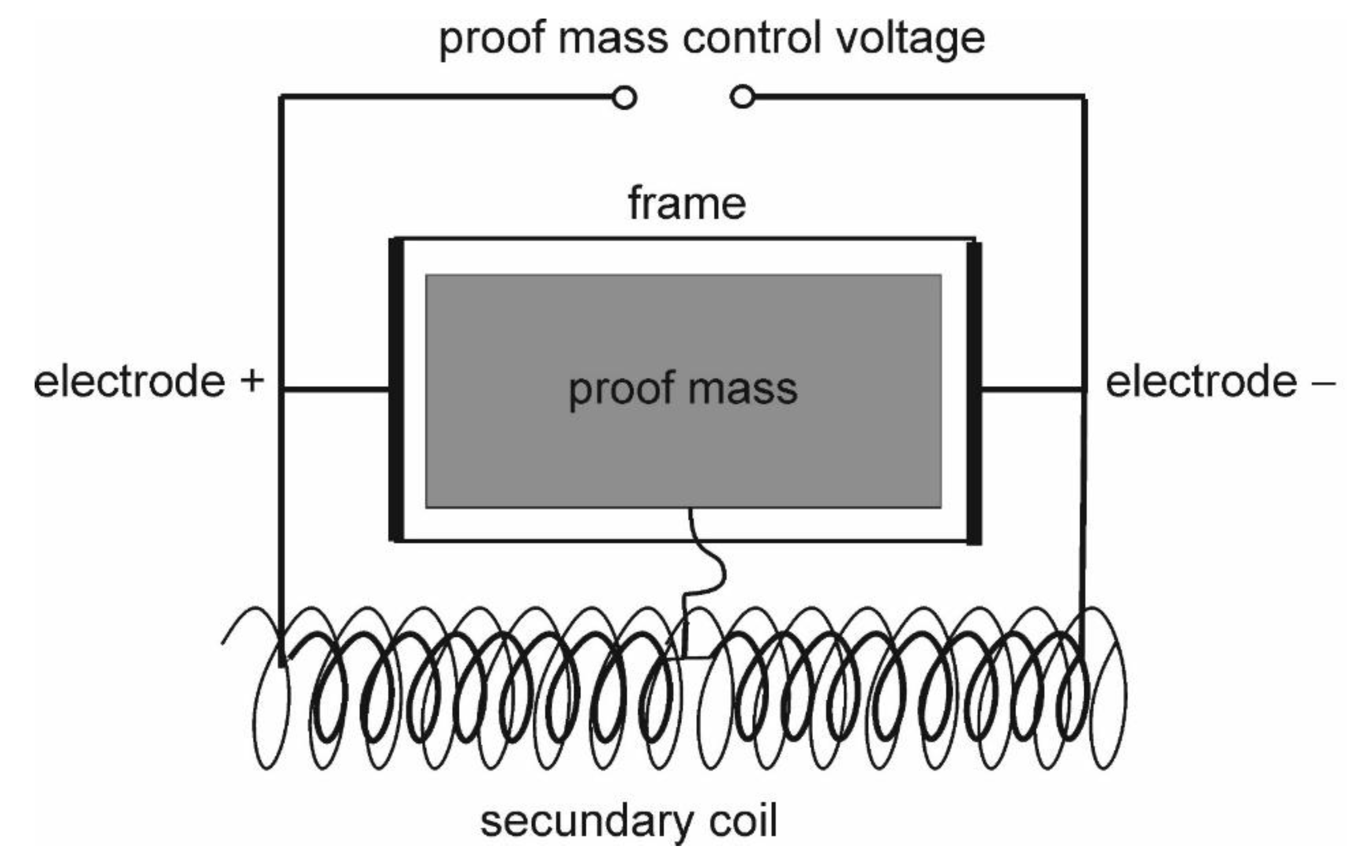
The GRACE SuperSTAR accelerometers, manufactured by ONERA [17], consist of a chromium coated titanium alloy proof mass of 4 × 4 × 1 cm3 free floating in a frame of ULE glass, where gold electrodes are coated. A servo-control loop controls the position and orientation of the proof mass in all six degrees of freedom in the cage. The proof mass is motionless in the middle of the cage when the electrostatic forces act. This is an instable equilibrium. The measured accelerations are proportional to the applied feedback force.
Figure 4 shows the schematic design for one axis. The proof mass is located between two electrodes, which are charged with the control voltage +Vc and −Vc, respectively. The frequency of the control circuit is 100 Hz. The charged proof mass has a voltage Vt consisting of the polarization voltage Vp and an alternating current, the detection voltage Vd.
Here, 100 kHz is the frequency of the detection voltage, too high to affect the motion of the proof mass. Two electric fields E1 and E2 build up between the walls of the proof mass and the electrodes. The accelerometer system is unstable. If the proof mass is charged positive and constant, the proof mass will move toward the electrode charged with −Vc. The gap between the proof mass and electrode is reduced, increasing the field and the attraction. A servo control is necessary to keep the proof mass motionless in this unstable position. It is the duty of the feedback loop to determine the voltage Vc necessary to keep the proof mass motionless at its nominal position. This voltage Vc is the measure for the acceleration of the satellite due to nonconservative forces and is between 1 µV and some V. A capacitive detector measures the position of the proof mass by comparing the capacitances. The large frequency difference between capacitive read-out and proof mass control, together with the lock-in detection, eliminates short high-frequency peaks entering the feedback loop. The whole accelerometer head is gold-coated and mounted inside an Invar housing for shielding static electric and magnetic fields, as Invar has a nearly “µ-metal” character.
The GRACE accelerometers have two ultrasensitive axes and one less sensitive to ensure testing of the instrument on ground with full gravity acting on the less sensitive axis. The gaps between the proof mass and electrode are about 100 µm small. On the GRACE mission, 10 Hz accelerometer data of all three axes are available. Table 1 summarizes the specification of the accelerometer axis.
Frequencies, which would significantly disturb the accelerometers, are well below the capacitive detection frequency of 100 kHz. The VLF band is below 10 kHz and, therefore, falls within the frequencies where the accelerometer is sensitive. Nevertheless, we suppose that the Invar housing shields the accelerometer head at least to electromagnetic fields in this frequency range.
GRACE is a NASA mission. The author does not know the test procedures conducted by NASA to test the magnetic and electric field, as well as the electro-magnetic compatibility tests. Procedures conducted by ESA concern [18] the susceptibility to magnetic fields at frequencies between 30 Hz and 100 kHz and to electric fields between 30 MHz and 18 GHz. Electromagnetic tests on the power leads are in the frequency range 30 Hz to 100 kHz. They also test the sensitivity to spike transients in the same frequency range. The susceptibility to higher electro-magnetic frequencies is tested on the power and signal lines. To the knowledge of the author, ESA does not emulate the ionosphere environment in these tests.
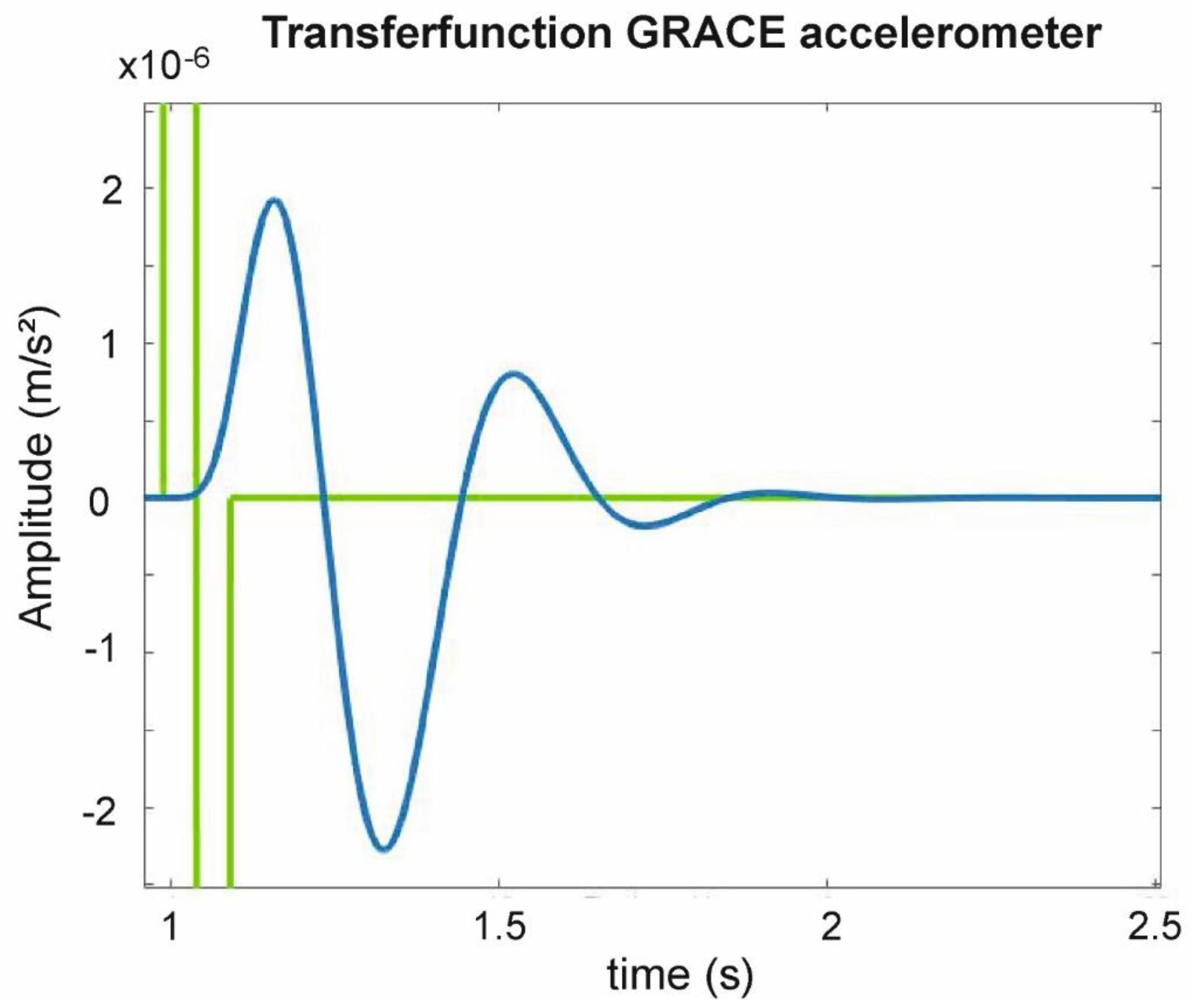
We already mentioned in the introduction, all disturbances on the GRACE accelerometers have a similar frequency content. The instrument itself sets an upper limit due to its transfer function. Figure 5 shows a response of the transfer function [19] to a sudden acceleration of the satellite or the proof mass. We want to emphasize here that even very sharp changes in acceleration, with frequency much lower than 100 kHz, do not excite the control loop to oscillations. The long-lasting oscillations in twangs are not synthetic from the accelerometer electronics.
2.2. Twangs and Their Detection
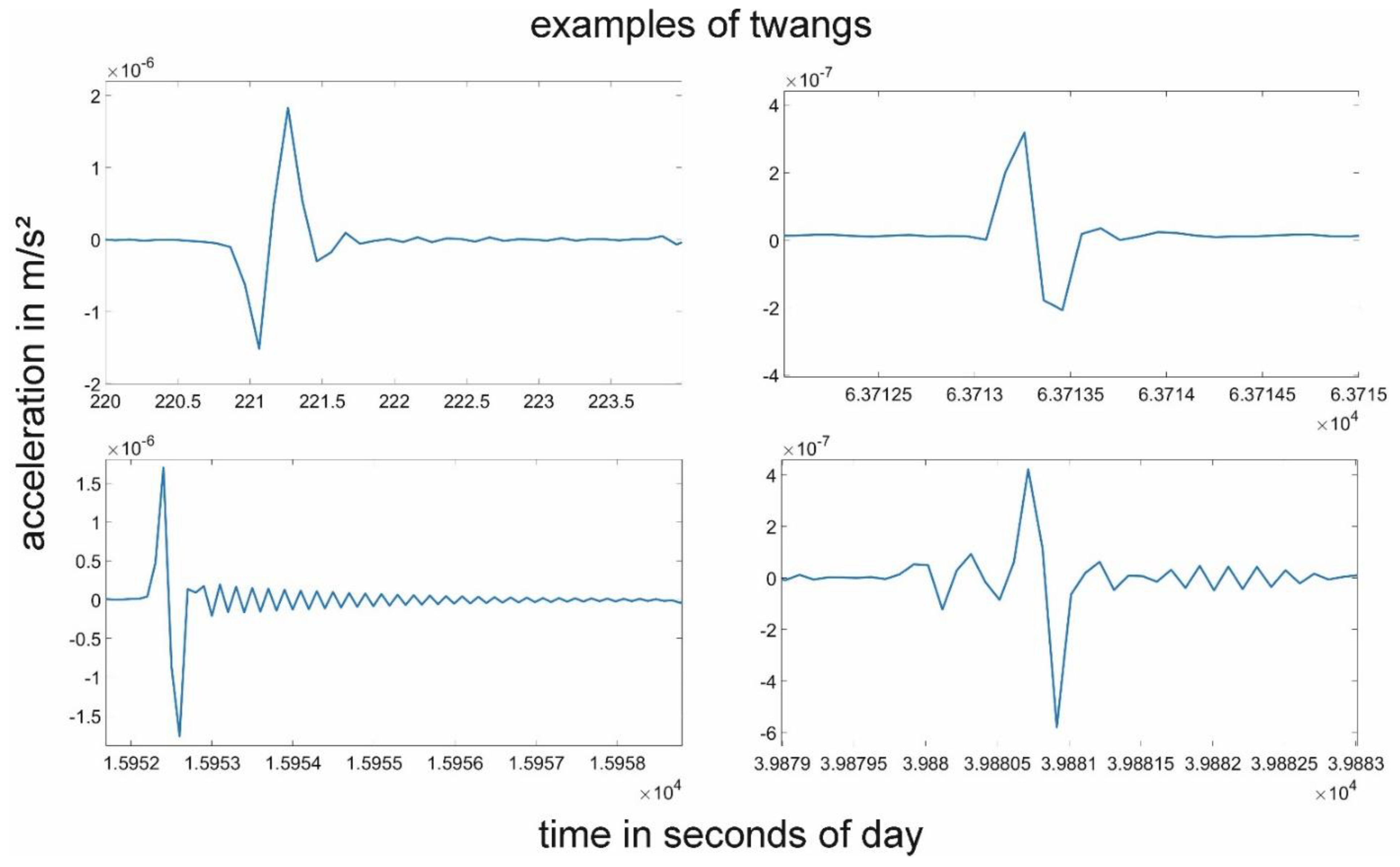
The strongest rapidly transient disturbances (at frequencies close to the read-out frequency of the accelerometer, i.e., 10 Hz) seen on satellite accelerometers of GRACE are the so-called “twangs”, sudden spikes with changing algebraic sign, often also called up-and-down spikes (up: positive down: negative). Sometimes they separate into two parts: the first part is a highly damped oscillation with high amplitudes, whereas the second part a slowly damped oscillation lasting up to 10 s (Figure 2). In contrast to other disturbances seen in these accelerometers [10,11], twangs have a variable shape; two-peak and three-peak or more structures exist, while a small precursor peak can sometimes be observed. The amplitude is variable, and some twangs show a following oscillation. The decaying tone of a vibrating string gives this phenomenon its name. Similar to the other disturbances, they have a time duration, indicating that the original signal is convoluted by the transfer function of the instrument [12]. Their biggest impact is on the radial direction (z-axis of the spacecraft). Following Hudson [20], twangs are the main reason for the high noise level of the radial component. There are a variety of shapes and sizes, typically around a few thousands of nm/s2, reaching up to 20,000 nm/s2 in the radial direction. In this early work, Hudson saw a geographical dependency of the occurrence of twangs together with trends in latitude and a correspondence with temperature (extracted from the Coarse Earth and Sun Sensor).
Peterseim [12] carried out a broad survey on the occurrence of twangs. Influenced by the work of Flury et al. [10] and Peterseim et al. [11], she detected twangs using the root mean square-ratio method introduced by Hudson [20], before resampling the signal to 100 Hz using a Gaussian reconstruction filter, and stacking many signals by cross-correlating the 100 Hz data. She identified two main types of twangs: positive when going up then down and negative if going down then up.
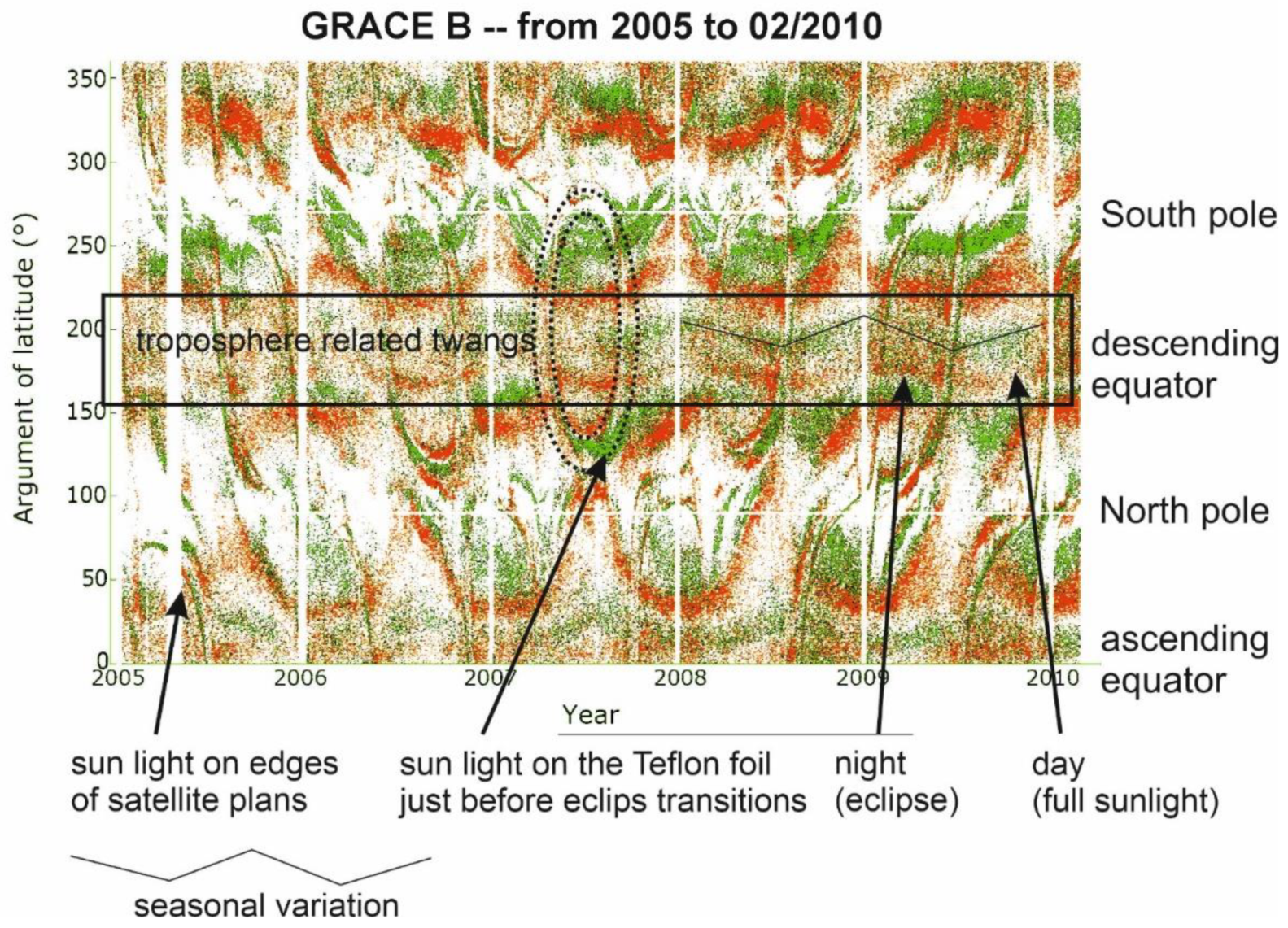
Peterseim [12] hypothesized that twangs can have different sources as some relate to clouds, while others relate to sunlight hitting different parts of the satellite structure. As her analysis did not separate the different sources, we summarize here some facts referring to cloud-related twangs. They represent the majority of these disturbances. Twangs show a seasonal, geographical, and local time variability, and the number of twangs differs on GRACE A and GRACE B. The number of twangs seen per day changes according to local time or eclipses, and there exists an increasing trend in the number of twangs, from the start of the mission in 2001 until early 2010 (end of analyzed data period). There are high-latitude twangs, but they occur less often, and nearly no twangs are seen close to the North and South Poles. In Figure 6, all detected twangs on GRACE B are plotted as a function of the argument of latitude for a period of some years. The twangs related to sunlight hitting certain surfaces of the spacecraft stick out, as they form sharp structures. The short period before an eclipse, when the sun hits the nadir foil, is marked as an oval. The majority of twangs at low and mid-latitudes are called cloud-related twangs in this study, as indicated in Figure 6. The variation in latitude with the season is marked as a zig-zag line. The GRACE orbit shows a precession movement; consequently, Figure 6 also shows a variation according to local time. At the equator crossing of the descending arcs in May 2008, for instance, the middle of the eclipse oval belongs to a local time near midnight changing linearly until the next eclipse phase, as indicated by the next oval structure. Figure 6 shows that the number of cloud-related twangs varies with local time. In the eclipses, the number of twangs is much higher than in the daytime.
When plotted with respect to the argument of latitude, positive and negative twangs form different bands (Figure 6). In a plot over time of the radial accelerometer data, the twangs occur in clusters. Within these clusters, positive and negative twangs alternate (see Figure 7a). Geographically, high-amplitude twangs form different bands, as shown in Figure 7b.
3. Results
In this section, we first summarize the facts known about the coupling of the ionosphere and the troposphere; then, we compare observations of twangs, selecting mostly cloud-related twangs, with the literature discussions on whistlers. Lastly, we focus on twangs around the equator. From the literature, it is known that whistlers observed in this region occur not far from lightning strikes, which inject them.
3.1. Troposphere and Ionosphere Coupling
The troposphere and the ionosphere are coupled systems. Sources for the coupling are planetary and gravity waves, Schumann and ionospheric Alfven resonances, and AC and DC electric field coupling (see the reviews in [21,22,23]). Only one of these coupling mechanisms relates to frequencies where the accelerometer is sensitive. The AC coupling between these two parts of the atmosphere relates the observations of sferics in the troposphere with whistlers in the ionosphere. The literature mentions lightning as the dominant source of whistlers, but it also discusses other natural phenomena, such as seismic activity, earthquakes, volcanic processes, and dust electrification. Singh [22] also mentions manmade contributions coming from power line emission, lightning triggering, thermonuclear explosions, and VLF and microwave transmitters. Different frequency intervals divide the electromagnetic spectrum into bands. Normally, only frequencies between 3 and 30 kHz belong to the very-low-frequency (VLF) domain. We do not distinguish between different bands in the electromagnetic spectrum, when we discuss the problem in this paper. Thus, only frequencies lower than the detection frequency of the accelerometer are important within the overall VLF range, i.e., mainly below 30 kHz.
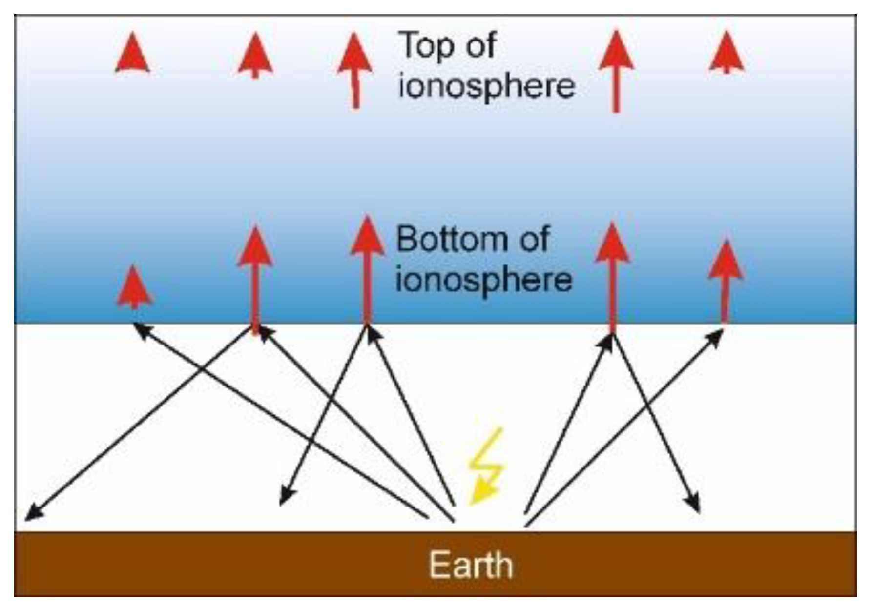
In the troposphere, the electromagnetic transients have the name sferics. They are impulse-type electromagnetic radiation caused by transient electric currents within lightning channels. The frequencies of these impulses are below 100 kHz. These waves propagate in the Earth ionosphere waveguide (Figure 8) in all directions around the Earth, and antennas detect them thousands of kilometers away from the thunderstorm from which they originated. Meteorologists use these signals, for instance, to register lightning strikes [24]. If the pulses, originating from lightning, couple into the magnetized ionosphere, they propagate in the whistler mode, if their frequency is below the electron plasma and gyro frequency. Thus, there exists a frequency limit of the propagation of a whistler in the ionosphere and magnetosphere. The limit is the plasma or gyro frequency, which is ever lower. The Earth magnetic field has a strong influence on the propagation mode; the propagation speed is low, and it varies with frequency. Propagation in the ionosphere and magnetosphere can happen in two different ways: ducted whistlers travel along the plasma density structure following magnetic field lines, while non-ducted whistlers travel in any direction relative to the magnetic field [25]. Whistlers, once injected into the ionosphere and traveling along the magnetic field lines, can reenter the troposphere. We hear a whistler when induced in long telephone cables on the ground as a decaying tone, just like a whistle blowing.
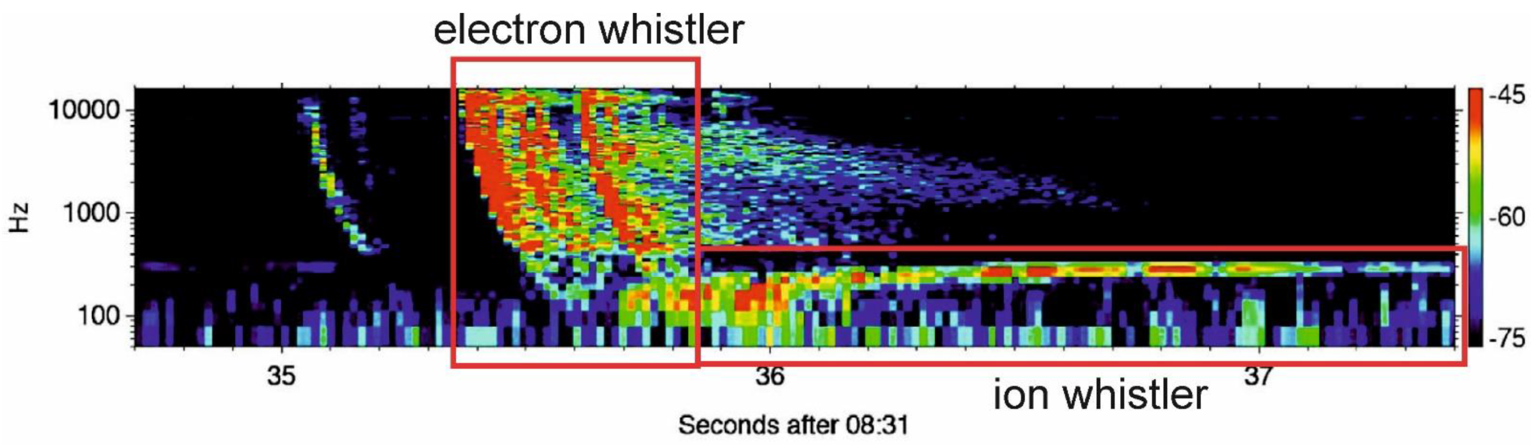
Figure 9 shows a typical measurement of a whistler on a satellite antenna [26]. The amplitudes of different frequency are color-coded. Sometimes, a whistler has two parts: the first part with rapidly decaying frequency and amplitude, i.e., the electron whistler; the second part with rising frequency and slowly decaying amplitude, i.e., the ion whistler. The frequency gap between these two whistler modes is the lower hybrid resonance.
One possible mechanism for the injection of whistlers is the coupling of sferics into the ionosphere. The sferics leave the Earth-ionosphere cavity as the reflection at the lower ionosphere boundary is not perfect. Using Snell’s law at the troposphere–ionosphere boundary, Hayakawa [25] concluded that frequencies below half of the electron plasma frequency can only penetrate into the ionosphere for very narrow transmission cones around a vertical wave normal angle. Figure 8 describes multiple injections of whistlers into the ionosphere. According to Hayakawa, ducted whistlers have at least the following characteristics: the frequency spectrum peaks at about 5 kHz, and the peak intensity is a few mV/m at mid-latitudes. Two factors control the occurrence rate of the whistlers in the ionosphere: how often lightning events occur, and the absorption rate along the propagation path. In the D- and E-regions of the ionosphere, whistler mode waves can be absorbed as electrons collide with neutral particles. On the way through the ionosphere, the formation of ducted whistlers takes place, and they propagate toward the pole. The plasma density in the ionosphere is not constant, but varies due to local time, as high energetic radiation from the sun leads to ionization. With the variation in the ionosphere plasma density, the occurrence rate of whistlers during the daytime is lower than that during the nighttime, with an additional peak at sunset at 20–30° latitude. The amplitude is lower in the daytime as absorption is higher. Hayakawa discussed the latitude dependence of whistlers; they should occur at latitudes between 10° and 60° with a maximum at 45° N and S. The limitation to 60° is due to injection by lightning strikes, which mostly occur in lower and mid-latitudes. The literature discussed a limitation of 10° due to the fact, that duct formation is more effective at mid-latitudes, while absorption loss is higher at low latitudes. Recently, Holzworth et al. [26] reported observations of non-ducted whistlers up to the magnetic equator, analyzing data from the Communication/Navigation Outage Forecast System (C/NOFS). Furthermore, whistlers show a seasonal variation due to the known asymmetry between thunderstorms in the northern and southern summer. We expect a geographical distribution of whistlers, as lightning strikes do not occur homogeneously around the globe. At the equator, thunderstorms occur in three distinct regions above South America, Africa, and Indonesia.
The study by Jacobson et al. [27] showed that relatively simple oblique non-ducted whistlers account for the majority of low-latitude whistlers. They also found that the coincidences between lightning strikes detected by the WWLLN and whistlers registered at the C/NOFS satellite (at a height between 400 km and 850 km) have a distance of 500 km to 10,000 km from the sub-satellite point with a maximum between 1000 and 4000 km. VLF bursts also occur at high latitude [28]. They have different sources, which are not discussed in this paper. We instead focus on whistlers at low and mid-latitudes.
In the ionosphere and magnetosphere, the electrons and ions are under the influence of the electromagnetic field of the wave. The additional force acting on moving charged particles leads to various propagation modes. Whistler mode waves have frequencies below the electron cyclotron or the electron plasma frequency. We distinguish between two whistler mode waves: the electron whistler, which has frequencies higher than the lower hybrid frequency; the ion whistler, with frequencies below this resonance. In the first case, the properties of the electrons have a greater influence, whereas, in the second case, the ion properties dominate.
The propagation mode of whistler waves is special. The electric field of the wave has a component parallel to the direction of propagation. The wave is not purely electromagnetic; it also has an electrostatic contribution. The amplitude of the electric field component in the direction of propagation depends on the frequency of the wave and is highest around the lower hybrid frequency. This fact may be important and could hint at an interaction with the accelerometer. This characteristic propagation mode should be taken into account when discussing electromagnetic compatibility on satellite missions.
Below, we compare the occurrence of whistlers with the detection of twangs in the accelerometer data. We focus on the behavior in terms of local time, latitude, and season and look for dispersion effects. The difficulties we face are the separation of different types of twangs, different influences on the whistler (occurrence of lightning, influence of the magnetic field absorption in the ionosphere), and the absence of any model describing the coupling to the accelerometer.
We want to compare whistlers with twangs; hence, we summarize the characteristics of whistlers in Table 2.
3.2. Comparison between Cloud-Related Twangs and Whistlers
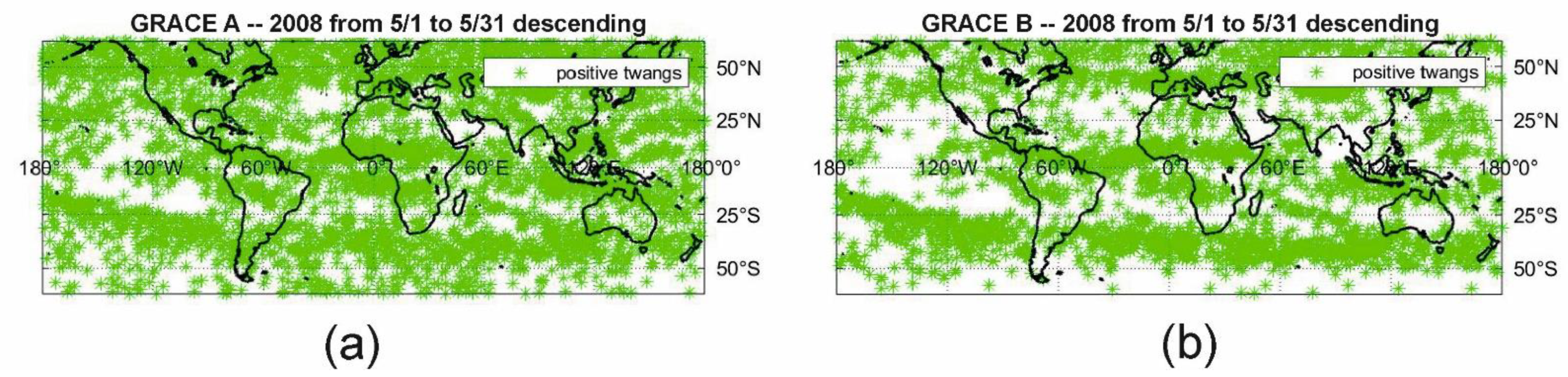
Twangs at low and mid-latitudes cannot be distinguished from high-latitude ones using the method of Peterseim [12], but they occur with different seasonal variation and latitude distribution depending on the local time. We focus on the lower latitudes in the discussion below. We also separate cloud-related twangs from other types and, therefore, restrict the analysis to eclipses, when no sunlit phenomena disturb our results. All other phenomena Peterseim linked to twangs are related to sunlight hitting the different surfaces of the satellite or switching the battery from loading to discharging. The fact that the number of twangs in eclipses is higher also makes the analysis more stable. Eclipses occurred in December and January 2007/2008 in the ascending tracks and in May/June 2008 in the descending tracks. We only show twangs in the radial direction, where their amplitude is highest. We classify twangs as positive or negative according to the first peak. We use the detection method described in Peterseim [12] and set the detection limit to a root-mean-square (rms) ratio of 1.17 (ratio between the rms of one second and the rms of the following second); therefore, only major twangs are registered. We focus on GRACE B, where we observed that the distinct troposphere-related structure of twangs is slightly more pronounced. On GRACE A, the observations are the same. Figure 10 shows the mid-latitude twangs for 1 month on GRACE A and GRACE B. The geographic pattern is comparable on both satellites.
The first similarity between twangs and whistlers is the asymmetry in number observed in the daytime and nighttime. For whistlers, this asymmetry is due to the fact that the E and D regions of the ionosphere, with a local time-dependent electron density, absorbs the whistler. Peterseim [12] previously observed that most twangs occur during the eclipse phases. To quantify this effect, we looked at 3 months in 2007–2008, i.e., November, December, and January, where the equator crossings occur between 11:00 a.m. and 2:00 p.m. and between 11:00 p.m. and 2:00 a.m. local time. We observed at low latitudes within ±25° only 1531 twangs in the daytime and 2545 twangs within the nighttime, although other disturbances could have corrupted the daytime value. The local time variability, as discussed by Peterseim, may be related to the absorption of whistlers in the ionosphere and the occurrence of lightning, which are seen more often in the evening than in the morning hours.
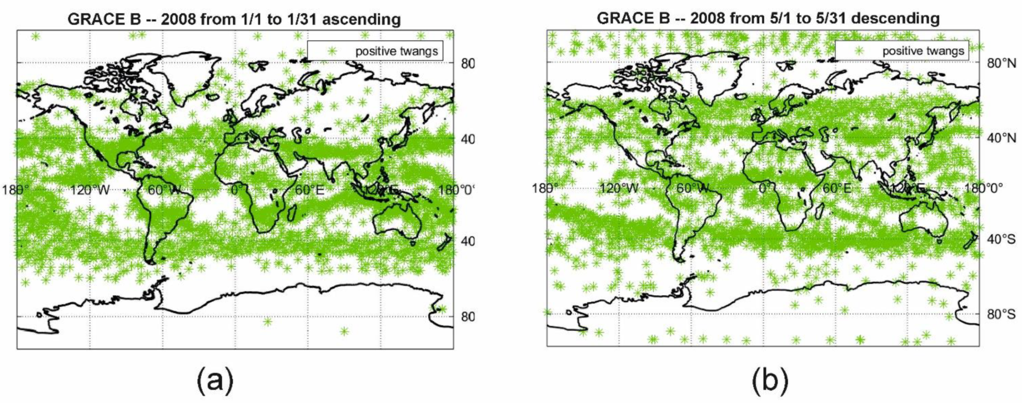
In Figure 11, we show the distribution of low and mid-latitude twangs in summer and winter. We can see the maximum number of twangs around 40–60° north and south, with fewer twangs at low latitudes. We can also observe that the whole latitude band of cloud-related twangs shifts slightly north in the northern summer (50° S–60° N) and shifts south in the northern winter (55° S–50° N). All these differences between summer and winter agree with what we discussed about the seasonal dependence of whistlers. We can explain the north and south shift with season by the fact that thunderstorms occur at higher latitudes in the summer hemisphere. The seasonal variation can be even better seen in Figure 6, where a zig-zag structure marks the shifting band.
The formation of whistlers depends on the magnetic field. The maximum numbers occur at latitudes of 40° to 60°. The maximum number of twangs is also located at these latitudes. We want to point out that Peterseim et al. [29] described a connection between the radial component of the magnetic field and the dependence on longitude of the northern mid-latitude band of twangs.
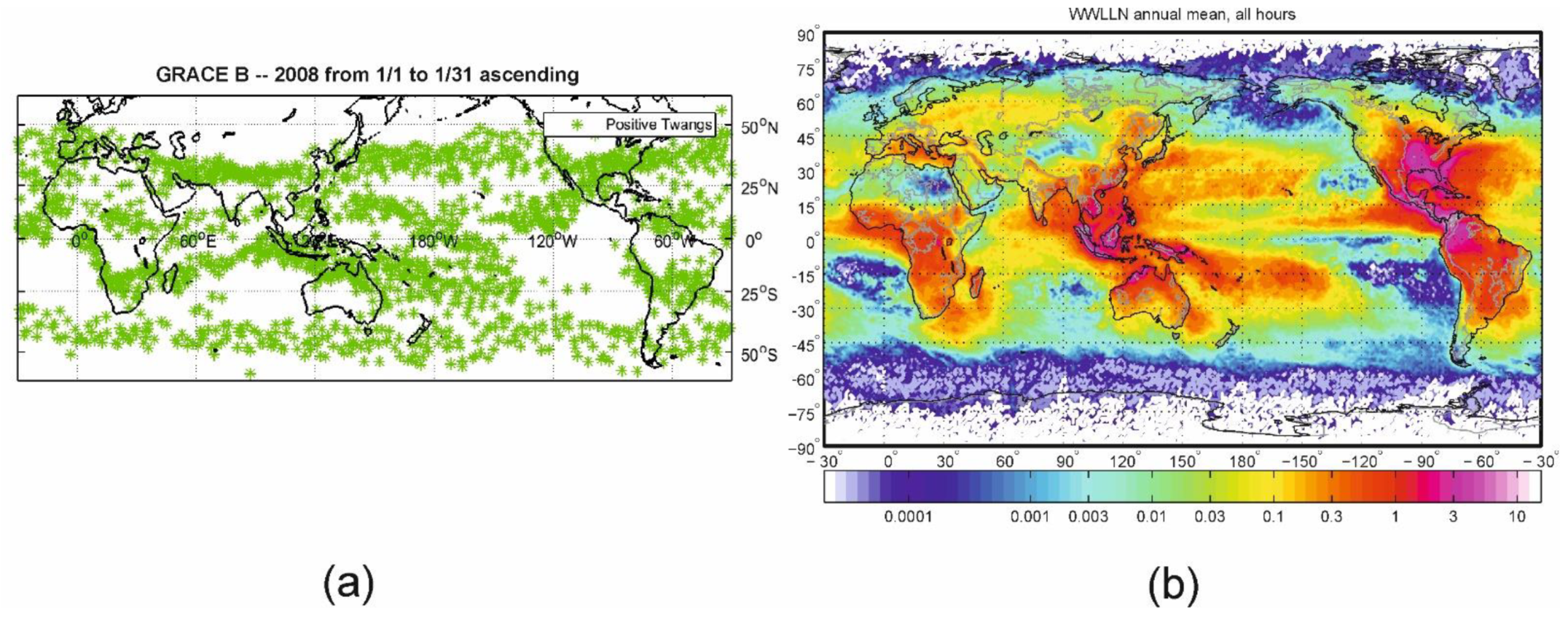
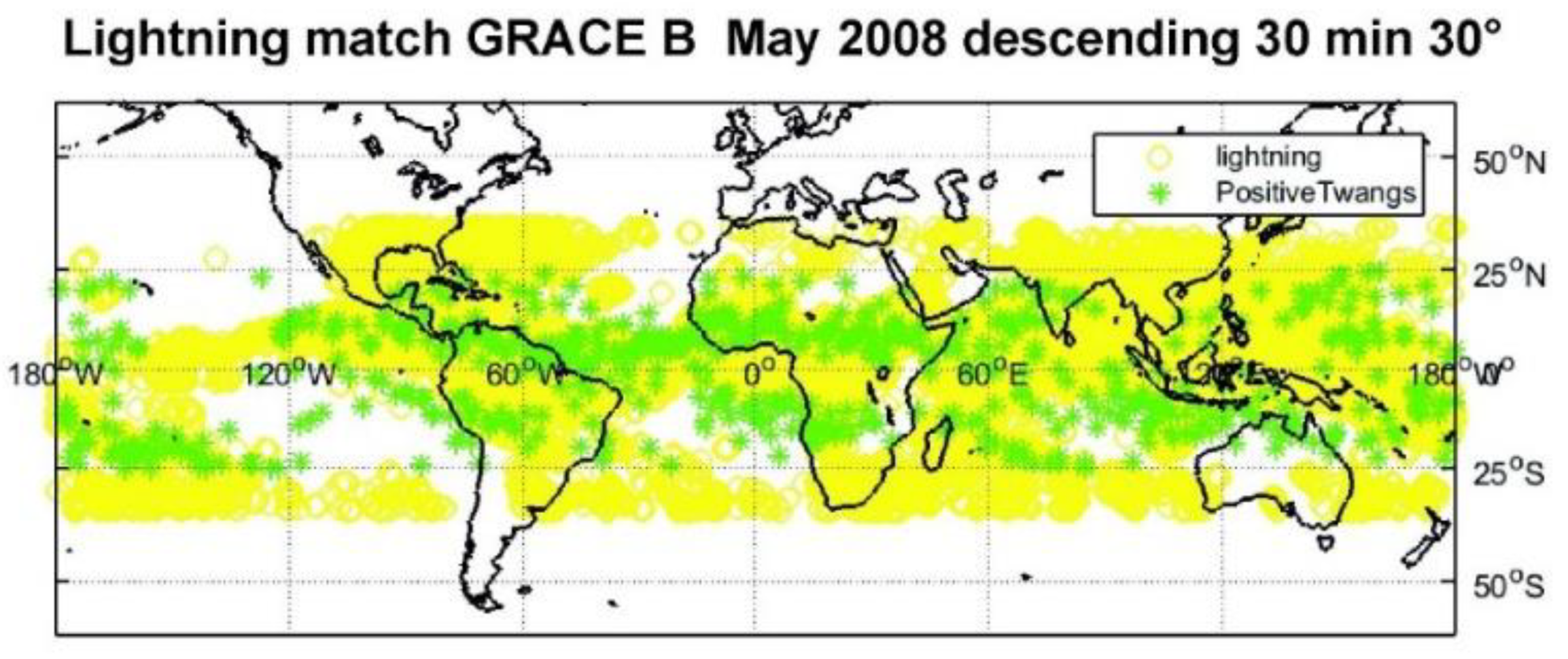
Figure 12 compares the occurrence of positive twangs on GRACE B for January 2008 with a global map of the mean number of lightning strikes detected by the WWLLN. As already mentioned in the last paragraph, whistlers detected on satellites correlate directly to lightning strikes at low latitudes [27], where the magnetic field in not optimal for coupling into the ionosphere. In mid-latitudes, sferics propagating a long distance within the Earth ionosphere cavity represent the perfect condition for coupling, and the geographical correlation is lost. A dominant feature observed by WWLLN corresponds to the longitudinal distribution of lightning, whereby nearly no lightning strikes are seen between Australia and Africa, between South Africa and South America, and between South America and about 130° west, leading to clustering. As seen in Figure 12a, this clustering also occurs in the distribution of twangs.
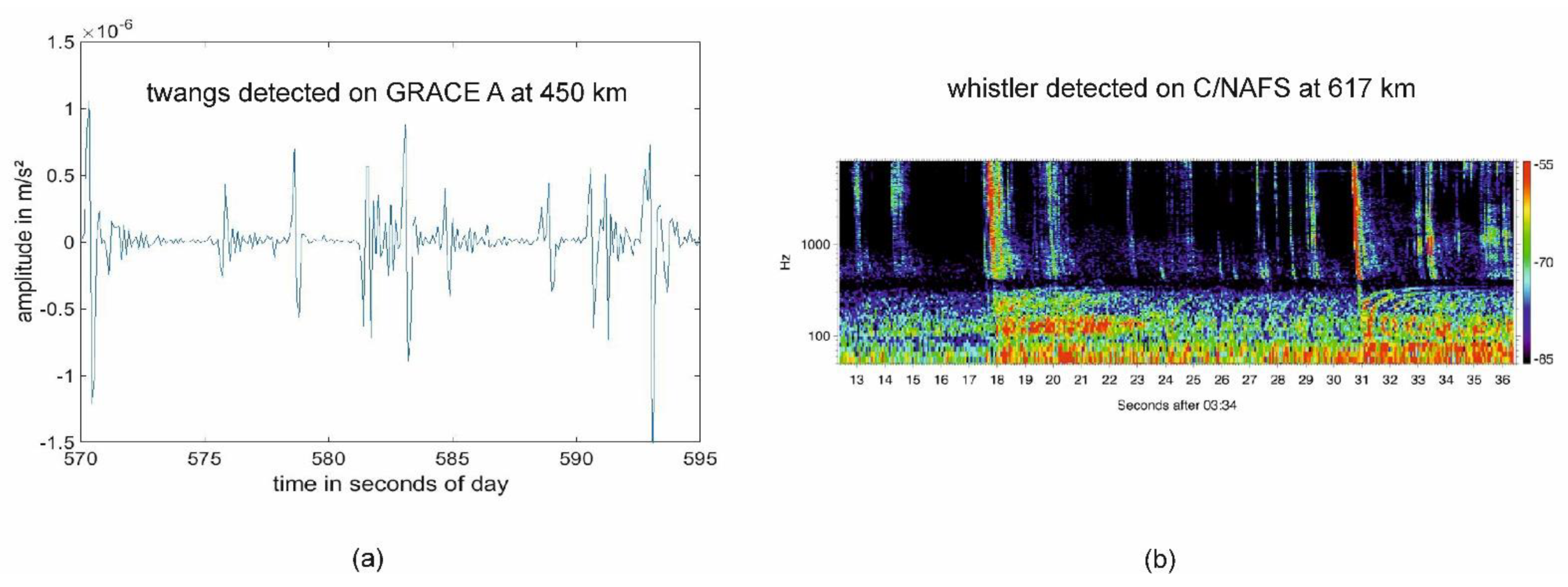
The rate of detection of whistlers on satellites and cloud-related twangs on GRACE B is a further indication for their connection. This parameter is dependent on the magnetic field orientation and has a latitude dependence. This dependency is small if we focus the analysis on the region around the equator. Other parameters include the sensitivity of the instruments and the rate of lightning, together with the coupling factor to the ionosphere. Figure 13a presents a timeseries of whistlers detected onboard of C/NOFS (height of 617 km) around the equator [26]. The detection rate was 0.6 s−1. Figure 13b shows a time series of detected twangs on GRACE at a height of 450 km. The detection rate was 0.4 s−1, comparable to the rate of whistlers on C/NOFS. The reader should be aware of the fact that these two figures have no relation in time. For this comparison, we want to highlight that the detection rate around the equator is comparable; thus, GRACE does not show many more twangs than the number of whistlers that would be detected by a dedicated satellite.
A characteristic of whistlers is that the dispersion along their path causes a spreading of the signal, which gives the burst its name. If we look for dispersion effects in the twangs, we first can see that twangs, in contrast to heater events [10] or torque spikes [11], have variable shapes and amplitudes (Figure 14). There are precursor pulses, pulses with extended duration, and even peaks followed by a damped oscillation, which explains the name twang. This oscillation can last up to 10 s, and its amplitude is lower than that of the previous peaks. We compare the first part of a twang, the rapidly decaying, high-amplitude oscillation with an electron whistler and the slowly decaying oscillation of lower amplitude lasting up to 10 s with the ion whistler (Figure 2 and Figure 7). The fact that more than one up-and-down peak occurs (contrary to the disturbance caused by the on-board heater and torque switching) can be a hint for dispersion.
Peterseim [12] reported that the number of twangs at the beginning of the mission was significantly lower than that toward the end of her analysis in 2010. The height of the GRACE satellites decayed successively, but less damping is not very likely to have causes this change in detection rate, as the absorption of whistlers takes place in the E and D region of the ionosphere and GRACE orbits in the F region. It seems that the coupling mechanism to the accelerometer changes with height.
3.3. Comparison between Cloud-Related Twangs and Lightning Strikes
In this section, we want to compare detected lightning strikes of the WWLLN with twangs at low altitudes (−25° to +25°). The WWLLN provides the location and time tagging of lightning strikes with a temporal accuracy of 30 µs and a spatial accuracy of about 15 km [31,32,33,34,35,36]). The difficulty in this comparison is that WWLLN only detects 7% of all global lightning. They detect only the biggest strikes. From every thunderstorm, lasting about 30 min to 1 h, at minimum of one big strike should be detected [37]. As on some satellite missions, where the coincidence between WWLLN-detected lightning and whistlers could be shown (e.g., [26,27]), we make a statistical analysis of possible coincidences of twangs and WWLLN-detected lightning.
The difficulty with respect to twangs lies in the time resolution of the accelerometer and the definition of an arrival time. The time best defined in a twang is the change in sign between the up and down peaks. If the signal is sampled at up to 100 Hz, this point can be marked within 20 ms. This time is definitely not the onset of a twang, which is uncertain by up to 0.5 s depending on the existence of precursor peaks. Furthermore, this onset of the twang is not the arrival time of the whistler. Further delays are due to the transfer function, as well as the effect of the sensor or even conversion times, as we cannot exclude that we do not detect the whistler itself, as it has to somehow couple to the satellite interior. The uncertainty in time between the arrival time of a whistler and the reaction time of the accelerometer makes a search for coincidences between twangs and lightning impossible.
A further uncertainty is the distance that the sferics travel before coupling into the ionosphere. According to Jacobson et al. [27], the majority of coincidences between on-board detected whistlers and WWLLN-located lightning strikes have a spatial distance between 1000 km and 4000 km. The large energy loss with distance (damping of 10−3 to 10−5) corresponds to a loss in quadratic distance-dependent electric field strength and causes the mean electric field of the whistler to fall by a factor of 1600 between 100 km and 4000 km. This seems to be realistic for the detection of twangs, which have an amplitude variability of at least three orders of magnitude.
Jacobson et al. [27] showed that, at low latitudes, simple oblique electron whistlers account for most VLF oscillations; hence, we restricted our analysis to ±25° latitude for the comparison with lightning strikes. This is also the region where we observed the highest relation to tropospheric structures. In this study, we had two months of data from the WWLLN, i.e., May and June 2008. We focused on the tracks when the satellite was in an eclipse, where fewer disturbances from other types of twangs, such as sun-induced discharges, were expected. In May and June, the descending tracks around the equator fulfilled this condition. We restrict the discussion to positive twangs, as they seemed to occur closer to the lightning strike.
To get a first view of this comparison, Figure 15 shows the occurrence of low- and mid-latitude positive twangs together with the lightning strikes detected at the WWLLN for May 2008. Nearly all twangs occurred in regions where lightning strikes were registered. It is interesting to note that twangs did not have high amplitudes in all geographical areas where lightning was detected. We can see fewer twangs mostly around the equator and in the Indian Ocean. As already discussed in Section 3.2, there are distinct regions where no positive twangs and no lightning occurred. These bands were between Australia and Africa (not so distinct in this period, but also not so distinct in the number of lightning strikes), between South Africa and South America, and between South America and about 130° west.
In Figure 15, only lightning strikes with a time delay of less than 30 min to the occurrence of the twang and a distance less than 30° in longitude and latitude are plotted (equivalent to the observations of Jakobson that most whistlers are found within a distance of 4000 km to the lightning strike). For 99–100% of the twangs, we could find at least one lightning strike, which fulfills this criterion. We could match only 57–65% of the twangs to a lightning strike if we limited the distance to 10°. The twangs which could not be related to a lightning strike seemed to cluster in different regions. For instance, the majority of negative twangs in Southeast Asia were not directly above Indonesia but shifted toward the west of Australia. These twangs lost a correlation.
In Table 3, we summarize the analysis with distance and time of separation. As expected for whistlers, we found that most twangs were related to lighting strikes within 30 min and a distance of 30°, with much fewer events when we restricted ourselves to shorter distances. Within 1 s before the twang, we could find, depending on distance, 3–19% of the twangs. Compared with the value of 7% of the lightning strikes detected by the WWLLN, this seems a reasonable number. The distance dependency is also reasonable. According to Jacobson et al. [27], the maximum correlation should exist between 3000 and 4000 km before a steep drop with smaller distances takes place.
4. Discussion
Accelerometers and data processing allow neither a very precise time resolution nor a precise definition of arrival time. Consequently, an analysis of coincidences between twangs and lightning is not possible. We focused in this paper on the characteristics of lightning and whistlers and compared their characteristics with observations on the occurrence of twangs. We grouped the common characteristics into four categories: the form of the twang, up to twangs which show a structure, which may be interpreted as electron and ion whistlers; geographical occurrence; daytime and nighttime variability; correlation to lightning and magnetic field. It must also be taken into consideration that we only analyzed high-amplitude twangs, as we had to introduce a threshold criterion for when a signal counts as a twang.
In contrast to any satellite-induced disturbance, the shape of cloud-related twangs is variable in its appearance. A twang can consist of two, three, or more peaks, with changing sign. It can have a precursor peak, as well as low amplitude, in addition to slowly decaying oscillations following the high-amplitude peaks and rapidly decaying main oscillation. We can interpret this behavior with the detection of more or less dispersed electron whistlers followed by ion whistlers. Cloud-related twangs can have positive or negative first peaks. As a slight difference, compared to lightning strikes in the troposphere, negative twangs appear slightly more spread than positive ones.
Different geographical, local time, and seasonal variations in the occurrence of twangs can also be used to characterize whistlers:
- Latitude variability: Whistlers that originate from lightning and low-latitude twangs occur between 60° north and south.
- Seasonal variability: The band shifts north in the northern summer.
- Bands predominant within 30–50° north and south: This is the region where the Earth magnetic field favors the coupling of the troposphere to the ionosphere. A structure related to the radial direction of the magnetic field was discussed in Peterseim et al [29].
- Clustering at the equator of low-latitude twangs in Indonesia, Africa, and Middle America with distinct gaps. At low latitude, where the magnetic field is not favorable for whistler formation, we expect a high geographic correlation with lightning.
- Day and night asymmetry: The damping of whistlers is less evident at nighttime, when the density of the ionosphere is lower, and more lightning strikes take place. We think that this is the reason for the local time variability of twangs.
- Repetition rate: the C/NOFS satellite detects whistlers with a comparable rate to twangs on GRACE B.
We performed a direct correlation between lightning strikes in the troposphere and twangs. We restricted this analysis to the latitudes within 25° north and south. In this region, the magnetic field is not favorable for the coupling of whistlers; hence, the correlation with the whistler source should be the highest. Nearly all twangs were related to a thunderstorm, where the lightning detected at the WWLLN was about 30 min (an approximation of the duration of a thunderstorm) before the detected twang within 30° spherical distance. Within 1 s, a correlation of 3–19% with WWLLN could be demonstrated (1.5° to 20° distance), which is also reasonable as the WWLLN only detects about 7% of lightning strikes. In summary, we can state that all variabilities, which we know from whistlers, appear with twangs, while the statistical evaluation is in an expected range.
Furthermore, no coincidences between lightning and twangs can be analyzed, and no quantitative study has been performed, due to the lack of a coupling mechanism between whistlers and accelerometer reaction. Thus, we conclude that it is very likely that whistlers cause twangs according to three considerations:
- The variability is the same.
- We know no other coupling mechanism between the troposphere and ionosphere, which is relevant.
- The accelerometers are sensitive in the VLF domain.
It is worth emphasizing that this analysis says nothing about the type of correlation between these phenomena. The correlation may be direct in the sense that there is an electromagnetic or electrostatic coupling to the sensor head or indirect in the sense that the accelerometer detects a mechanical excitation.
Are there satellite specific effects that hint at the coupling mechanism? GRACE A shows much more twangs than GRACE B and has a higher asymmetry in the number of cloud-related twangs between noon and midnight. At low latitudes, the detected twangs show the same characteristics as on GRACE B. There are spacecraft-specific features even in twin satellites, but they seem to be related to the amplitude of the response of the accelerometer, as opposed to different sources.
Can we learn something from the direction-dependent disturbance? Twangs have the highest amplitude in the radial direction. This coincides with the propagation direction of the whistlers. Non-ducted whistlers, injected into the ionosphere by sferics, propagate nearly in the radial direction. This is a great angle to the magnetic field; consequently, these whistlers have a great component of the electric field in the direction of propagation. A direct coupling of the electric field into the accelerometer may be a possibility. An Invar housing shields the accelerometer from electrostatic and electromagnetic disturbances. A follow-up study of the behavior of metals and other materials as a function of the special whistler propagation mode in the ionosphere seems necessary as motivated by this study. A necessary discussion on how VLF influences the accelerometer will only be possible after such a study. The same applies for the amplitude of the reaction of the accelerometer. We can state that a voltage of mV in the frequency range of 100 Hz and below will cause an acceleration of at least 1000 nm/s2. It is, therefore, detectable by the accelerometer.
5. Conclusions
We must explicitly state that this paper does not prove that whistlers are the reason for twangs; however, many observations hint to a correlation, and no other phenomenon is known to couple the troposphere and ionosphere, leading to transients in the frequency range within which the accelerometer is sensitive. The importance of this study lies in the fact that a sensitivity to VLF and frequencies below is outside the standard test procedures of space instruments, and we have no tests for the interaction of plasma waves with materials used in space. In plasmas, electrostatic waves can be excited. We have to include tests for these special types of waves. A sensitivity of space accelerometers or satellite structures to VLF and below would help to explain all the disturbances related to switching processes in the spacecraft; these switching processes induce plasma waves in a frequency range and propagation mode not considered in electromagnetic compatibility tests. The tests do not cover VLF, they do not cover electrostatic waves, and they do not take into account the plasma environment of the instruments.
Funding
This research was funded by Deutsche Forschungsgemeinschaft, grant number AOBJ:649679.
Data Availability Statement
The data presented in this study are available on request from the corresponding author. The data are not publicly available due to the fact, that the underlying accelerometer data from JPL is not publicly available.
Acknowledgments
The authors wish to thank the World Wide Lightning Location Network (http://wwlln.net), a collaboration among over 50 universities and institutions, for providing the lightning location data used in this paper. The author also specially thanks Reiner Rummel who supported this work in many ways and followed the discussion with interest.
Conflicts of Interest
The authors declare no conflict of interest.
References
- Bai, Y.; Li, Z.; Hu, M.; Liu, L.; Qu, S.; Tan, D.; Tu, H.; Wu, S.; Yin, H.; Li, H.; et al. Research and Development of Electrostatic Accelerometers for Space Science Missions at HUST. Sensors 2017, 17, 1943. [Google Scholar] [CrossRef] [PubMed]
- Touboul, P.; Foulon, B.; Christophe, B.; Marque, J.P. CHAMP, GRACE, GOCE instruments and beyond. In Geodesy for Planet Earth; Kenyon, S., Pacino, M., Marti, U., Eds.; Springer: Berlin, Germany, 2012; pp. 215–221. [Google Scholar]
- Friis-Christensen, E.; Lühr, H.; Hulot, G. Swarm: A constellation to study the Earth’s magnetic field. Earth Planets Space 2006, 58, 351–358. [Google Scholar] [CrossRef] [Green Version]
- Drinkwater, M.R.; Floberghagen, R.; Haagmans, R.; Muzi, D.; Popescu, A. GOCE: ESA’s first Earth Explorer Core mission. In Earth Gravity Field from Space—From Sensors to Earth Sciences; Space Sciences Series of ISSI; Beutler, G.B., Drinkwater, M.R., Rummel, R., von Steiger, R., Eds.; Kluwer Academic Publishers: Dordrecht, The Netherlands, 2003; Volume 18, pp. 419–432. ISBN 1-4020-1408-2. [Google Scholar]
- Hudson, D.; Chhun, R.; Touboul, P. Development status of the differential accelerometer for the MICROSCOPE mission. Adv. Space Res. 2007, 39, 307–314. [Google Scholar] [CrossRef]
- Dolesi, R.; Bortoluzzi, D.; Bosetti, P.; Carbone, L.; Cavalleri, A.; Cristofolini, I.; DaLio, M.; Fontana, G.; Fontanari, V.; Foulon, B.; et al. Gravitational sensor for LISA and its technology demonstration mission. Class. Quantum Gravity 2003, 20, 99–108. [Google Scholar] [CrossRef]
- Armano, M.; Audley, H.; Auger, G.; Baird, J.T.; Bassan, M.; Binetruy, P.; Born, M.; Bortoluzzi, D.; Brandt, N.; Caleno, M.; et al. Sub-Femto-g Free Fall for Space-Based Gravitational Wave Observatories: LISA Pathfinder Results. Phys. Rev. Lett. 2016, 116, 231101. [Google Scholar] [CrossRef] [Green Version]
- Gruenwaldt, L.; Meehan, T. CHAMP Orbit and Gravity Instrument Status. In First CHAMP Mission Results for Gravity, Magnetic and Atmospheric Studies; Reigber, C., Lühr, H., Schwintzer, P., Eds.; Springer: Berlin, Germany, 2003; pp. 3–10. [Google Scholar]
- Gruenwaldt, L.; Bock, R. Heater Switching Procedure and Test Results; Technical Report CH-GFZ-TR-2201; GFZ Potsdam: Potsdam, Germany, 2000. [Google Scholar]
- Flury, J.; Bettadpur, S.; Tapley, B. Precise accelerometry on board the GRACE gravity field satellite mission. Adv. Space Res. 2008, 42, 1414–1423. [Google Scholar] [CrossRef]
- Peterseim, N.; Flury, J.; Schlicht, A. Magnetic torquer induced disturbing signals within GRACE accelerometer data. Adv. Space Res. 2012, 49, 1388–1394. [Google Scholar] [CrossRef]
- Peterseim, N. TWANGS—High-Frequency Disturbing Signals in 10 Hz Accelerometer Data of the GRACE Satellites. Ph.D. Thesis, Verlag der Bayerischen Akademie der Wissenschaften, Munich, Germany, 2014. [Google Scholar]
- Bonin, G.R.; Orr, N.G.; Zee, R.E.; Cain, J. Solar Array Arcing Mitigation for Polar Low-Earth Orbit Spacecraft. In Proceedings of the 24th Annual AIAA/USU Conference on Small Satellites, Logah, UT, USA, 9–12 August 2010. [Google Scholar]
- Siemes, C.; de Teixeira da Encarnacuo, J.; Doornbos, E.; van den Ijssel, J.; Kraus, J.; Perestry, R.; Grunwaldt, L.; Apelbaum, G.; Flury, J.; Olsen, P.E.H. Swarm accelerometer data processing from raw accelerations to thermospheric neutral densities. Earth Planets Space 2016, 68, 92. [Google Scholar] [CrossRef] [Green Version]
- Behzadpour, S.; Mayer-Gürr, T.; Krauss, S. GRACE follow-on accelerometer data recovery. J. Geophys. Res. Solid Earth 2021, 126, e2020JB021297. [Google Scholar] [CrossRef]
- Tzamali, M.; Peidou, A.; Pagiatakis, S. GRACE-FO and Swarm integrated data analysis reveals ionospheric disturbances on the accelerometer meaurements. In Proceedings of the EGU General Assembly Conference, Online, 4–8 May 2020. EGU2020-12931. [Google Scholar]
- Frommknecht, B.; Oberndorfer, H.; Flechtner, F.; Schmidt, R. Integrated sensor analysis for GRACE – development and verfication. Adv. Geosci. 2003, 1, 57–63. [Google Scholar] [CrossRef] [Green Version]
- ECSS European Cooperation for Space Standardization, ECSS_E-ST-20-07C Space Engineering: Electromagnetic compatibility Rev 2, 3 January 2022. Available online: https://ecss.nl/standard/ecss-e-st-20-07c-rev-2-electromagnetic-compatibility-3-january-2022/ (accessed on 13 April 2022).
- Bettadpur, S. Brief Note on the ACC Transfer Function & Its Application to Simulated Drag Time Series; Note; Center for Space Research, University of Texas at Austin: Austin, TX, USA, 2000. [Google Scholar]
- Hudson, D. In-Flight Characterization and Calibration of the SuperSTAR Accelerometer. Master’s Thesis, The University of Texas at Austin, Austin, TX, USA, 2003. [Google Scholar]
- Simões, F.; Pfaff, R.; Berthelier, J.; Klenzing, J. A review of low frequency electromagnetic wave phenomena related to tropospheric-ionospheric coupling mechanisms. Space Sci. Rev. 2012, 168, 551–593. [Google Scholar] [CrossRef] [Green Version]
- Singh, A.K. Diagnostic features of VLF waves in terrestrial magnetosphere. Adv. Geosci. 2011, 27, 31–40. [Google Scholar]
- Barr, R.; Llanwayn Jones, D.; Roger, C.J. ELF and VLF radio waves. J. Atmos. Sol. Terr. Phys. 2000, 62, 1689–1718. [Google Scholar] [CrossRef]
- Dowden, R.L.; Brundell, J.B.; Rodger, C.J. VLF lightning location by time of group arrival (TOGA) at multiple sites. J. Atmos. Sol. Terr. Phys. 2002, 64, 817–830. [Google Scholar] [CrossRef]
- Hayakawa, M. Whistlers. In Handbook of Atmospheric Electrodynamics; Volland, H., Ed.; CRC Press: Boca Raton, FL, USA, 2002; ISBN 0-8493-2520-X (v. 2). [Google Scholar]
- Holzworth, R.H.; McCarthy, M.P.; Pfaff, R.F.; Jacobson, A.R.; Willcockson, W.L.; Rowland, D.E. Lightning-generated whistler waves observed by probes on the Communication/Navigation Outage Forecast System satellite at low latitudes. J. Geophys. Res. 2011, 116, A06306. [Google Scholar] [CrossRef] [Green Version]
- Jacobson, A.R.; Holzworth, R.H.; Pfaff, R.F.; McCarthy, M.P. Study of oblique whistlers in the low-latitude ionosphere, jointly with the C/NOFS satellite and the World-Wide Lightning Location Network. Ann. Geophys. 2011, 29, 851–863. [Google Scholar] [CrossRef] [Green Version]
- Labelle, J.; Treumann, R.A. Auroral radio emissions, 1. Hiss, Roars, and Bursts. Space Sci. Rev. 2002, 101, 295–440. [Google Scholar] [CrossRef]
- Peterseim, N.; Schlicht, A.; Flury, J. Improved Acceleration Modelling and Level 1 Processing Alternative for GRACE. In GEOTECHNOLOGIEN Science Report; Münch, U., Dransch, W., Eds.; GEOTECHNOLOGIEN: Potsdam, Germany, 2010; Volume 17, pp. 31–34. [Google Scholar] [CrossRef]
- Virts, K.S.; Wallace, J.M.; Hutchius, M.L.; Holzworth, R.H. Highlights of a new ground-based, hourly global lightning climatology. Bull. Am. Meteo. Soc. 2013, 94, 1381. [Google Scholar] [CrossRef] [Green Version]
- Jacobson, A.R.; Holzworth, R.H.; Harlin, J.; Dowden, R.; Lay, E. Performance assessment of the World Wide Lightning Location Network (WWLLN), using the Los Alamos Sferic Array (LASA) array as ground-truth. J. Atmos. Ocean. Technol. 2006, 23, 1082–1092. [Google Scholar] [CrossRef]
- Lay, E.H.; Jacobson, A.R.; Holzworth, R.H.; Rodger, C.J.; Dowden, R.L. Local time variation in land/ocean lightning flash density as measured by the World Wide Lightning Location Network. J. Geophys. Res. 2007, 112, D13111. [Google Scholar] [CrossRef] [Green Version]
- Lay, E.H.; Holzworth, R.H.; Rodger, C.J.; Thomas, J.N.; Pinto, O.; Dowden, R.L. WWLLN global lightning detection system: Regional validation study in Brazil. Geophys. Res. Lett. 2004, 31, L03102. [Google Scholar] [CrossRef] [Green Version]
- Rodger, C.J.; Werner, S.; Brundell, J.B.; Lay, E.H.; Thomson, N.R.; Holzworth, R.H.; Dowden, R.L. Detection efficiency of the VLF World-Wide Lightning Location Network (WWLLN): Initial case study. Ann. Geophys. 2006, 24, 3197–3214. [Google Scholar] [CrossRef] [Green Version]
- Rodger, C.J.; Brundell, J.B.; Dowden, R.L. Location accuracy of VLF World-Wide Lightning Location (WWLL) network: Post-algorithm upgrade. Ann. Geophys. 2005, 23, 277–290. [Google Scholar] [CrossRef] [Green Version]
- Rodger, C.J.; Brundell, J.B.; Dowden, R.L.; Thomson, N.R. Location accuracy of long distance VLF lightning location network. Ann. Geophys. 2004, 22, 747–758. [Google Scholar] [CrossRef] [Green Version]
- Holzworth, R.H.; University of Washington, Washington, DC, USA. Personal communication, 2018.
Figure 1.
The 10 Hz read out of a high sensitivity axis of the GOCE accelerometer A2. The dominant signature is a result of the heater switching. The heaters are connected in series in three lines. Every line switches every second, as the heaters are pulse modulated. The time between switching of two different lines is 1/3 s.

Figure 2.
A twang in the accelerometer measurements consisting of two parts. The first part is a high amplitude oscillation, which is followed by an oscillation with smaller amplitude that decays more slowly.
Figure 2.
A twang in the accelerometer measurements consisting of two parts. The first part is a high amplitude oscillation, which is followed by an oscillation with smaller amplitude that decays more slowly.

Figure 3.
Timeseries of the accelerometer measurements on Swarm B (x red, y green, z blue, x and z shifted). The abrupt changes in the accelerometer bias lead to steps in the measurements. The steps accompany very high spike disturbances.
Figure 3.
Timeseries of the accelerometer measurements on Swarm B (x red, y green, z blue, x and z shifted). The abrupt changes in the accelerometer bias lead to steps in the measurements. The steps accompany very high spike disturbances.

Figure 4.
Sketch of one axis of the accelerometer read-out and control.

Figure 5.
With the help of the transfer function (according to [19]) the response of the accelerometer to a rectangular up-and-down peak with 10−5 m/s2 and a duration of 20 ms can be calculated. The input acceleration is shown in green, and the response of the accelerometer is shown in blue.
Figure 5.
With the help of the transfer function (according to [19]) the response of the accelerometer to a rectangular up-and-down peak with 10−5 m/s2 and a duration of 20 ms can be calculated. The input acceleration is shown in green, and the response of the accelerometer is shown in blue.

Figure 6.
Detected twangs on the accelerometer in radial direction of GRACE B with argument of latitude. Positive twangs are marked in green, while negative twangs are marked in red. Positive spikes go up then down, while negative spikes go down then up. We can relate sharp structures to sun illumination of individual surfaces of the satellite. We mark the eclipse phase by an oval when sun hits the nadir foil. The number of twangs varies between daytime and nighttime. A seasonal variation in latitude of cloud-related twangs is marked by the zig-zag structure.

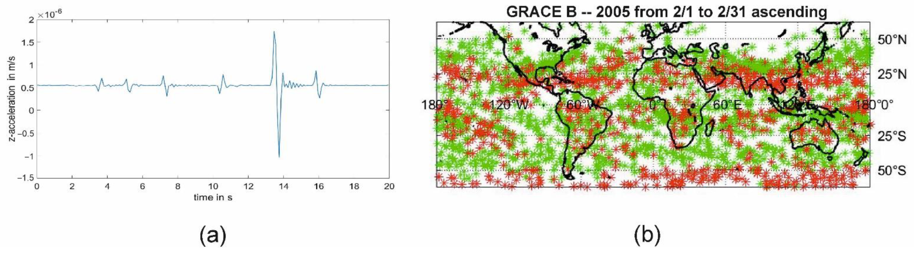
Figure 7.
Twangs often occur as multiples with a changing sign. Left, a sequence of twangs on GRACE B is shown (a). Looking at the geographical distribution of positive (green) and negative (red) twangs (right), the different types form different bands, where high-amplitude negative twangs can be separated from high-amplitude positive twangs (b).

Figure 8.
Coupling of sferics into the ionosphere.

Figure 9.
A whistler can consist of two parts: a high-frequency part with decaying frequency, i.e., the electron whistler; a low-frequency part with increasing frequency, i.e., the ion whistler. The frequency gap between these two parts is the lower hybrid resonance. The measurements were taken from Holzworth et al. [26]. The figure shows the detected frequency against time. The amplitude of the signal is color-coded.

Figure 10.
Comparison of the geographical structure of twangs between GRACE A (a) and GRACE B (b).

Figure 11.
Summer (b) and winter (a) asymmetry of the occurrence of twangs on GRACE B in 2007/2008. The figure shows only positive twangs. The mid-latitude band of cloud-related twangs occurs in the winter between 60° S and 40° N and in the summer between 40° S and 60° N.
Figure 11.
Summer (b) and winter (a) asymmetry of the occurrence of twangs on GRACE B in 2007/2008. The figure shows only positive twangs. The mid-latitude band of cloud-related twangs occurs in the winter between 60° S and 40° N and in the summer between 40° S and 60° N.

Figure 12.
A comparison between the geographical occurrence of high-amplitude positive twangs (a) and the annual mean occurrence of lightning strikes (b) detected by the World Wide Lightning Location Network (WWLLN, right, [30] © American Meteorological Society). In the region between 25° north and south, the dominant areas where twangs and lightning occur are South and Middle America, Africa, and Indonesia. Gaps of twangs and lightning are visible at the same locations, between South America and −130°, between Australia and Africa, and between Africa and South America. The main difference is the band of twangs within 40–50° north and 40–50° south, where the magnetic field is favorable for the coupling of sferics into the ionosphere.

Figure 13.
Comparison of the principal rate of twangs detected on GRACE (a) with the rate of whistlers detected on C/NAFS (b). These two plots are not taken at the same epoch nor at the same longitude. They simply serve as a comparison around the equator [26].
Figure 13.
Comparison of the principal rate of twangs detected on GRACE (a) with the rate of whistlers detected on C/NAFS (b). These two plots are not taken at the same epoch nor at the same longitude. They simply serve as a comparison around the equator [26].

Figure 14.
Twangs have varying shapes. In most cases, they consist of double or triple peaks, but more peaks can also occur. An oscillation following the peaks is as common as a precursor peak or even precursor oscillation. These examples are taken from GRACE B on 25 April 2003. The two twangs on top show the two distinct parts of a twang, the high amplitude oscillation with a rapid decay and the following low amplitude oscillation with slow decay.

Figure 15.
Geographical plot of positive twangs between 25° north and south in May 2008 together with lightning strikes detected by the World Wide Lightning Location Network (WWLLN), which occurred within a distance of 30° and a timespan of 30 min around the location and detection time of the twang.


Table 1.
SuperSTAR accelerometer specification.
| Axis | Range in m/s2 | Accuracy in m/(s2√Hz) |
|---|---|---|
| x | ±5 × 10⁻⁵ | 1 × 10⁻¹⁰ |
| y | ±5 × 10⁻⁴ | 1 × 10⁻⁹ |
| z | ±5 × 10⁻⁵ | 1 × 10⁻¹⁰ |
Table 2.
Characteristics of whistlers.
| Category | Description |
|---|---|
| Shape | Two parts: Electron whistler Ion whistler |
| Day-night asymmetry | Absorption in E and D layers of ionosphere |
| Geography | Low and mid-latitudes, Shifting north or south with season |
| Correlations | Lightning Magnetic field |
Table 3.
List of lightning strikes detected by WWLLN for different distances in time and space to positive, nighttime twangs detected on GRACE B. WWLLN data were available for 2 months, May and June 2008.
Table 3.
List of lightning strikes detected by WWLLN for different distances in time and space to positive, nighttime twangs detected on GRACE B. WWLLN data were available for 2 months, May and June 2008.
| Time/Distance between Lightning and Twang | May 2008 (Total: 618 Positive Twangs) Number of Matches (Percentage) | June 2008 (Total: 922 Positive Twangs) Number of Matches (Percentage) | |||
|---|---|---|---|---|---|
| ±30 min | 30° | 616 | 100 | 912 | 99 |
| 20° | 612 | 99 | 898 | 97 | |
| 10° | 355 | 57 | 599 | 65 | |
| 5° | 337 | 55 | 558 | 61 | |
| 3° | 240 | 39 | 397 | 43 | |
| 1.5° | 125 | 20 | 201 | 22 | |
| −3 s | 30° | 276 | 61 | 512 | 56 |
| 20° | 246 | 40 | 360 | 39 | |
| 10° | 92 | 15 | 161 | 17 | |
| 5° | 38 | 6 | 62 | 7 | |
| 3° | 18 | 3 | 24 | 3 | |
| 1.5° | 8 | 1 | 7 | 0.8 | |
| −1 s | 30° | 207 | 33 | 296 | 32 |
| 20° | 118 | 19 | 184 | 20 | |
| 10° | 38 | 6 | 79 | 9 | |
| 5° | 13 | 2 | 31 | 3 | |
| 3° | 8 | 1 | 7 | 0.8 | |
| 1.5° | 4 | 0.6 | 3 | 0.3 | |
Publisher’s Note: MDPI stays neutral with regard to jurisdictional claims in published maps and institutional affiliations. |
© 2022 by the author. Licensee MDPI, Basel, Switzerland. This article is an open access article distributed under the terms and conditions of the Creative Commons Attribution (CC BY) license (https://creativecommons.org/licenses/by/4.0/).
Share and Cite
MDPI and ACS Style
Schlicht, A. GRACE Accelerometers Sensitive to Ionosphere Plasma Waves: Similarities between Twangs and Whistlers. Geosciences 2022, 12, 228. https://0-doi-org.brum.beds.ac.uk/10.3390/geosciences12060228
AMA Style
Schlicht A. GRACE Accelerometers Sensitive to Ionosphere Plasma Waves: Similarities between Twangs and Whistlers. Geosciences. 2022; 12(6):228. https://0-doi-org.brum.beds.ac.uk/10.3390/geosciences12060228
Chicago/Turabian StyleSchlicht, Anja. 2022. "GRACE Accelerometers Sensitive to Ionosphere Plasma Waves: Similarities between Twangs and Whistlers" Geosciences 12, no. 6: 228. https://0-doi-org.brum.beds.ac.uk/10.3390/geosciences12060228
Note that from the first issue of 2016, this journal uses article numbers instead of page numbers. See further details here.