
Tsunamis Generated and Amplified by Atmospheric Pressure Waves Due to an Eruption over Seabed Topography


Graduate School of Science and Engineering, Kagoshima University, Kagoshima 890-0065, Japan
Geosciences 2022, 12(6), 232; https://0-doi-org.brum.beds.ac.uk/10.3390/geosciences12060232
Submission received: 8 April 2022
/
Revised: 24 May 2022
/
Accepted: 28 May 2022
/
Published: 31 May 2022
(This article belongs to the Special Issue Interdisciplinary Geosciences Perspectives of Tsunami Volume 4)
Abstract
:Numerical simulations were generated using a nonlinear shallow-water model of velocity potential to study the fundamental processes of tsunami generation and amplification by atmospheric pressure waves. When an atmospheric pressure wave catches up with an existing tsunami that is propagating as a free wave over an abrupt change in water depth, the amplified tsunami propagates in the shallower water. An existing tsunami propagating as a free wave over a sloping seabed is also amplified by being passed by atmospheric pressure waves. When atmospheric pressure waves travel over an abrupt change in water depth, the water surface profile of tsunamis in the shallower water depends on both the interval of the atmospheric pressure waves and the phase of the tsunami-generation process over the change in water depth. Moreover, when atmospheric pressure waves travel over an abrupt change in water depth, the tsunami amplitude in the shallower water increases, as the water depth of the shallower area is decreased and the Proudman resonance is further reduced. When an atmospheric pressure wave train with positive pressure travels over a sloping seabed, the amplification of tsunami crests propagating as free waves is controlled by leaving the forced water waves following the atmospheric pressure waves. Conversely, the amplitudes of tsunami troughs propagating as free waves increase.
1. Introduction
Tsunamis were widely observed—especially along the Pacific coasts—when the large eruption of Hunga Tonga–Hunga Ha’apai volcano occurred in January 2022. On the Japanese coasts, the tsunamis appeared two or three hours earlier than their predicted arrival time. Such tsunamis were not incorporated into the forecast system of the Japan Meteorological Agency, so the tsunami warnings were issued using the conventional warning system in response to the beginning of anomalous fluctuations in the tide records. After the eruption, the atmospheric Lamb wave with the largest pressure deviation of approximately 2 hPa was observed in Japan [1]. Therefore, one of the sources that caused the tsunamis observed far away from the eruption site was considered to be the Proudman resonance [2], which is also an origin of meteotsunamis, e.g., [3]. The tsunamis caused by atmospheric pressure fluctuations due to eruptions were studied for the 1883 Krakatau volcanic eruption tsunamis [4,5,6,7,8,9,10,11], as well as the 1956 Bezymianny volcanic eruption tsunamis [12,13].
The investigations of the 2022 Hunga Tonga–Hunga Ha’apai volcanic eruption tsunamis were started soon after the event; for example, the relationship between the atmospheric pressure waves and resultant tsunamis was studied using numerical models [14,15,16]. The numerical results indicated that the initial fluctuations in the tide level and the atmospheric pressure waves were closely related in each region. The tsunamis caused by the topographic changes due to the volcanic eruption were also simulated numerically [17]. Moreover, both local and global tsunamis have begun to be summarized, e.g., [18,19].
However, the amplification mechanism of tsunamis with a total amplitude of more than 2 m—as was observed at Amami, Japan [1]—is still unknown. Furthermore, the generation and amplification mechanisms of tsunamis by multiple atmospheric pressure waves have not been clarified. This is because the main source of meteotsunamis was usually considered to be only an atmospheric pressure wave due to a weather disturbance when the Proudman resonance was examined for the meteotsunamis observed along various coasts of the world, e.g., [20,21,22,23,24]. Conversely, in the atmospheric pressure fluctuations due to a volcanic eruption, it is known that an atmospheric Lamb wave is followed by a large number of atmospheric pressure waves, including atmospheric gravity waves, which travel slower than the atmospheric Lamb wave [1].
In the present study, as a fundamental study on air–sea waves, we investigated the generation and amplification processes of tsunamis due to multiple atmospheric pressure waves. We considered several steady atmospheric pressure waves traveling at a constant velocity, and generated numerical simulations by applying a nonlinear shallow-water model of the velocity potential of tsunamis. We set model seabed topography with an abrupt change in water depth or a uniform slope, and investigated the effects of these topographies on the tsunamis due to an atmospheric pressure wave train. After explaining both the numerical methods and conditions in Section 2, we present the amplification of an existing tsunami caught up or passed by atmospheric pressure waves in Section 3. In Section 4, we describe the effects of stepped and sloping seabed topographies on tsunamis generated by an atmospheric pressure wave train. In Section 5, we give a brief discussion of the tsunamis’ sources by referring to both the tide-gauge and atmospheric pressure records at Amami, Japan, in the wake of the 2022 Hunga Tonga–Hunga Ha’apai volcanic eruption.
2. Numerical Method and Conditions
2.1. Numerical Method and Atmospheric Pressure Wave Model
We consider the irrotational motion of an inviscid and incompressible fluid. When considering the pressure p(x, t) at the water surface, the nonlinear shallow-water equations of the velocity potential ϕ(x, t) are described as follows:
where η(x, t) and b(x) are the water surface displacement and seabed position, respectively, and ∇ is a horizontal partial differential operator, namely, (∂/∂x, ∂/∂y). The gravitational acceleration g is 9.8 m/s2, and the sea water density ρ is 1030 kg/m3.
In this study, we consider the one-dimensional propagation of waves along the x-axis direction. Equations (1) and (2) were solved numerically using a finite difference method with central and forward difference schemes for space and time, respectively. The grid size Δx was 500 m, whereas the time step interval Δt was 0.7 s. The initial value of velocity potential, ϕ(x, 0 s), was 0 m2/s at any location.
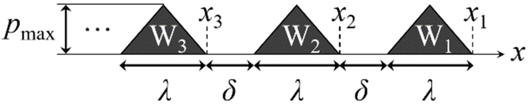
In order to investigate the fundamental effects of atmospheric pressure waves on the generation and amplification processes of tsunamis, we introduced a model of atmospheric pressure waves, as in the numerical calculations with a linear shallow-water model [15], because the actual atmospheric pressure waves show complicated wave profiles. That is, it was assumed that the steady atmospheric pressure waves as depicted in Figure 1 traveled in the positive direction of the x-axis at the same constant traveling velocity vp. The profile of the atmospheric pressure waves was an undeformed isosceles triangle with positive pressure. The interval between the atmospheric pressure waves was δ, and the location of the onshore end of the nth atmospheric pressure wave Wn was xn at the initial time, i.e., t = 0 s.
In the computation, the triangle height—i.e., the maximum value of atmospheric pressure, pmax—was 2 hPa for any of the atmospheric pressure waves. Although it may be excessive to set the atmospheric pressure to 2 hPa for atmospheric pressure waves due to an eruption other than an atmospheric Lamb wave, it is a standard value for pressure fluctuations that generate meteotsunamis. In this study, to investigate the effects of multiple atmospheric pressure waves, we performed model calculations with a larger maximum value of atmospheric pressure and, conversely, a limited number of atmospheric pressure waves.
For the verification of the numerical model, tsunamis were numerically generated by an atmospheric pressure wave W1, as illustrated in Figure 1, traveling over water with a uniform still-water depth of h, for a duration of time τ. After the atmospheric pressure wave W1 stopped traveling and a tsunami generated by W1 left from W1, the maximum amplitude of the tsunami propagating as a free wave, namely, ηmax, was numerically obtained. The calculated ηmax was compared with the estimated maximum amplitude of the corresponding tsunami under the linear shallow-water condition, namely, ζmax, which was obtained by Equation (8) in [3], i.e.,
where the units of atmospheric pressure, length, and time are Pa, m, and s, respectively.
ζmax = [pmax·(vpτ)/(λ/2)]/20000,
We considered cases in which the wavelength λ and travel duration τ of an atmospheric pressure wave were 10 km and 210 s, respectively. When the still-water depth h was 2000 m and the traveling velocity vp of the atmospheric pressure wave was = 140 m/s, the maximum water level ηmax at t = 2800 s was 0.072 m after the atmospheric pressure wave stopped traveling at t = 210 s. Conversely, the corresponding ζmax was 0.059 m. Furthermore, when h was 5000 m and vp was ≃ 221 m/s, the maximum water level ηmax at t = 2800 s was 0.095 m, whereas ζmax was 0.093 m. Although relatively good results were obtained numerically, the results using the nonlinear shallow-water model were larger than the corresponding values from Equation (3) for linear shallow-water waves, and the difference between the two was larger in the shallower water.
Moreover, we considered cases in which the still-water depth h was 2000 m and the traveling velocity vp and duration τ of an atmospheric pressure wave were = 140 m/s and 300 s, respectively. When the wavelength of the atmospheric pressure wave, λ, was 30 km, the maximum water level ηmax at t = 340 s using the nonlinear shallow-water model was 0.034 m. Conversely, the corresponding value χmax obtained using the Boussinesq-type equations [25], which are described as Equations (A1) and (A2) in the Appendix A, was also 0.034 m at t = 340 s. Furthermore, when the wavelength of the atmospheric pressure wave, λ, was 20 km, the maximum water level ηmax was 0.051 m, and χmax was 0.045 m, at t = 340 s.
If the wavelength of atmospheric pressure waves is shorter over deeper water, the dispersion of tsunamis will increase, and the tsunami height will decrease. When using different governing equations, the following may cause differences in calculation results:
- (1)
- The phase velocity of a tsunami that effectively resonates with atmospheric pressure waves with the same traveling velocity over water with the same depth may be different.
- (2)
- In the tsunami-generation process, free-wave components may be evaluated differently.
- (3)
- In the tsunami-propagation process, tsunami profiles are calculated differently when traveling as free waves after leaving the atmospheric pressure waves.
In several other cases with conditions similar to those in the above cases, the calculations were not stopped by instability even over a discontinuity in water depth, and the tsunami height differences due to the wave dispersion were within approximately 12%. Therefore, based on these results, a nonlinear model without considering the wave dispersion, as well as the Coriolis force and seabed friction, was applied for simplicity, to study the fundamental mechanisms of tsunamis generated by atmospheric pressure waves.
In the following calculations, instead of an atmospheric Lamb wave traveling at the front, we consider subsequent atmospheric pressure waves such as atmospheric gravity waves to investigate the effects of multiple atmospheric pressure waves. The traveling velocity vp of every atmospheric pressure wave was set to 250 m/s, which was slower than the atmospheric Lamb wave with a traveling velocity over 300 m/s [1]. The length of the atmospheric pressure waves, λ, indicated in Figure 1 was 10 km.
2.2. Seabed Topography
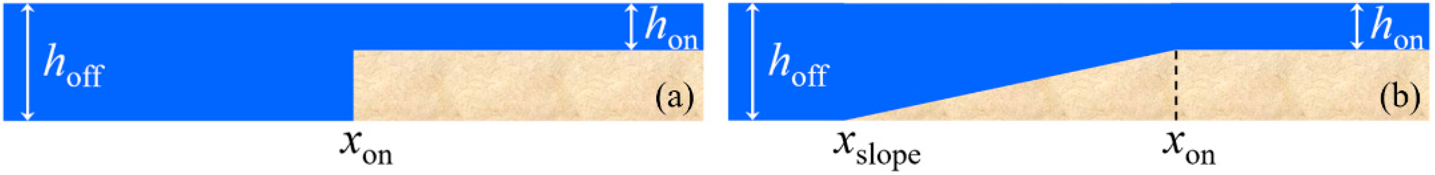
Figure 2 depicts two types of seabed topography in the numerical experiments. The still-water depth in the deepest offshore area is denoted by hoff, which was 5000 m in every calculation, whereas that in the shallowest onshore area is hon. Figure 2a presents a stepped seabed, in which the water depth is discontinuous at x = xon. Conversely, Figure 2b illustrates a seabed including a slope with a constant gradient β at xslope ≤ x ≤ xon.
The calculation conditions are listed in Table 1.
3. Amplification of an Existing Tsunami Caught up or Passed by Atmospheric Pressure Waves over Seabed Topography
3.1. Amplification of an Existing Tsunami Caught up by an Atmospheric Pressure Wave over an Abrupt Change in Water Depth
In Section 3, we consider the cases in which subsequent atmospheric pressure waves chase a tsunami, TLamb, generated by a preceding atmospheric Lamb wave and propagating as a free wave. In the computation, the tsunami TLamb was generated by setting the water level η(x, 0 s) at 60 km ≤ x ≤ 70 km to 0.06 m. After the initial time t = 0 s, two tsunamis with a height of approximately 0.03 m propagated in both the positive and negative directions of the x-axis. The former was called TLamb, which was chased by atmospheric pressure waves.
We first consider an atmospheric pressure wave chasing an existing tsunami in Case A. The seabed topography was stepped, as depicted in Figure 2a, in which the still-water depth in the onshore shallower area, hon, was 2000 m, and the offshore end of the onshore shallower area was located at xon = 170 km. The atmospheric pressure wave was W1, as illustrated in Figure 1, in which x1 is 55 km. The conditions of Case A are described in Table 1.
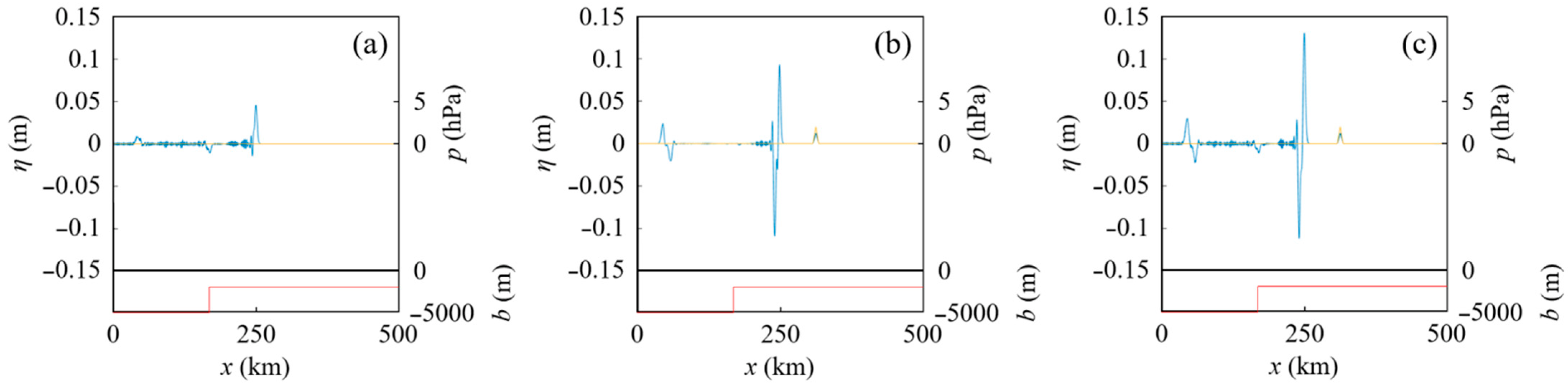
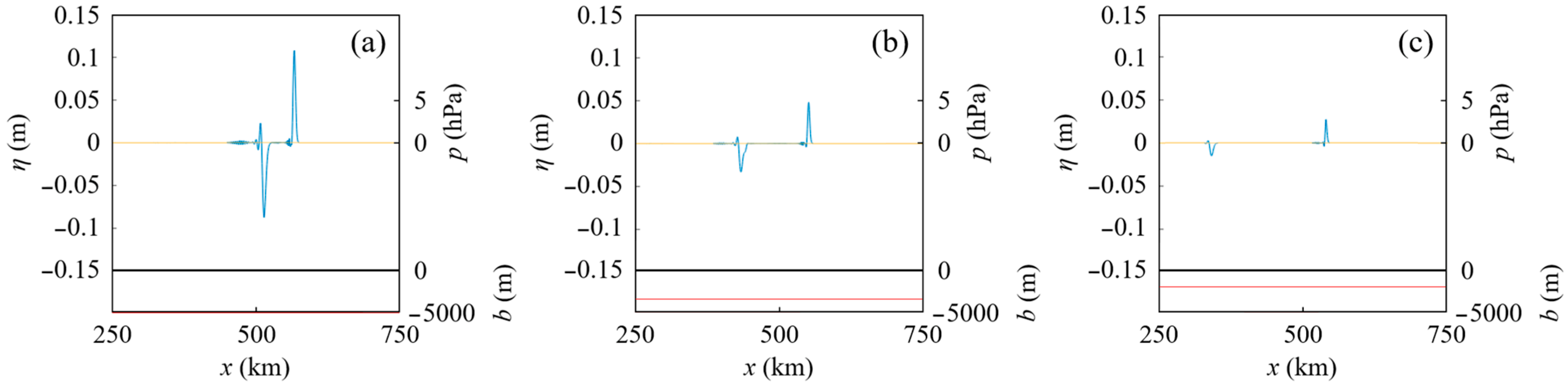
When W1 catches up with the existing tsunami TLamb over the abrupt change in water depth, the water surface profile at t = 1050 s is presented in Figure 3c. Conversely, Figure 3a depicts the corresponding water surface profile of the tsunami TLamb propagating in the positive direction of the x-axis, without any atmospheric pressure wave, while Figure 3b depicts the corresponding result due to the atmospheric pressure wave W1 without the tsunami TLamb.
Figure 3b indicates, from the right, a forced wave and transmitted free waves propagating in the positive direction of the x-axis in the shallower water, and also depicts reflected free waves propagating in the negative direction of the x-axis in the deeper water. In the present paper, a water wave that follows an atmospheric pressure wave is called a forced wave even if it contains a free-wave component with a recovery force of gravity in the resonance process. The maximum amplitudes of the crests of the transmitted and reflected free waves were at = 0.093 m and ar = 0.023 m, respectively. Conversely, based on the linear shallow-water theory [8], at = 0.083 m and ar = 0.019 m, so the results of the present numerical model were both slightly larger.
In the case of Figure 3c, when the existing tsunami TLamb entered the shallower water, the atmospheric pressure wave W1 caught up with TLamb, and the crest generated and amplified by W1 was superimposed on TLamb. Thereafter, W1 left TLamb in the shallower water, bringing only the forced wave component, the wave height of which was not large because the Proudman resonance was not effective in the shallower water. Therefore, the amplified tsunami was propagating in the shallower water, as depicted in Figure 3c. In the present results, the maximum water levels at t = 1050 s are 0.045m, 0.093 m, and 0.13 m in Figure 3a–c, respectively. When an atmospheric Lamb wave is followed by a large number of atmospheric pressure waves, including atmospheric gravity waves, the chances of tsunami height amplification due to such topographic changes increase.
3.2. Amplification of an Existing Tsunami Passed by Atmospheric Pressure Waves over a Sloping Seabed
Second, we consider atmospheric pressure waves passing an existing tsunami in Case B, the conditions of which are described in Table 1. The seabed topography included a uniform slope, as depicted in Figure 2b, in which there was a slope with a constant gradient of β = 6.25 × 10⁻³ at 20 km ≤ x ≤ 500 km.
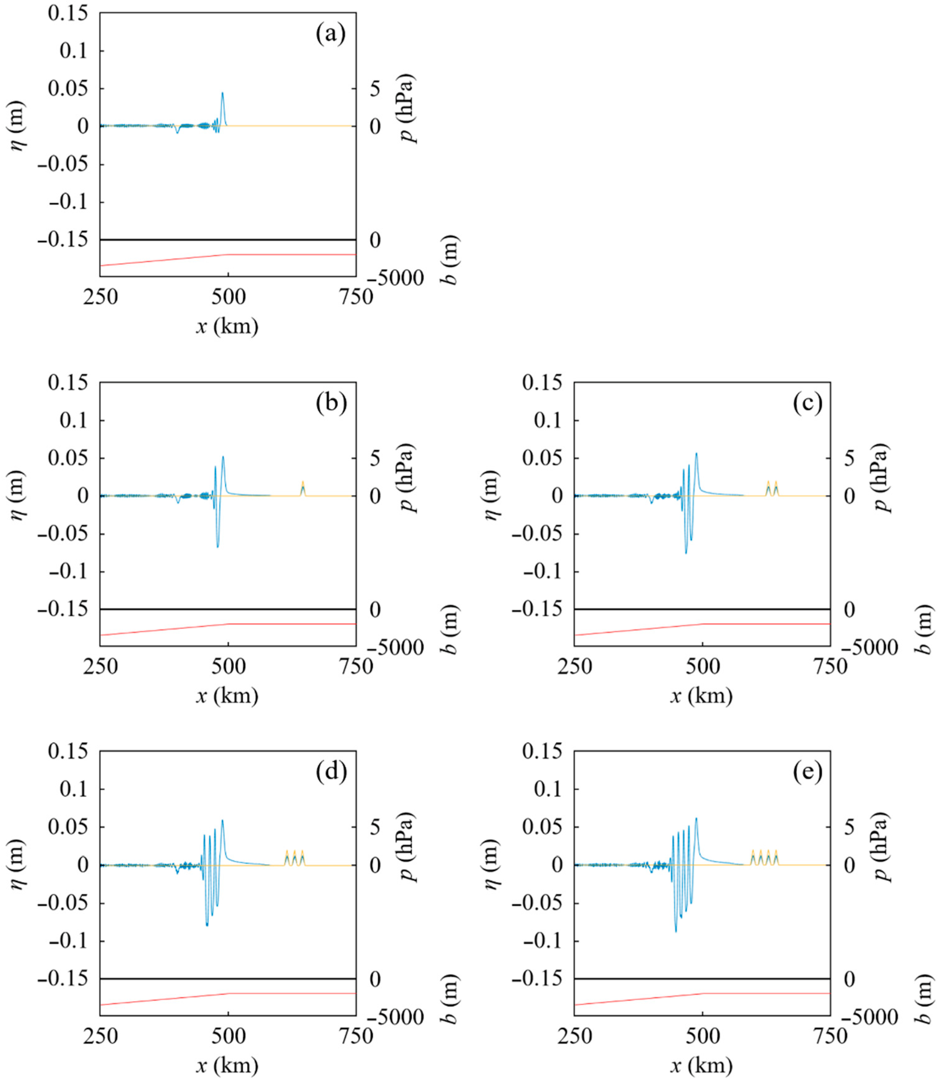
When the atmospheric pressure waves as illustrated in Figure 1—in which x1 is 55 km and the interval δ is 5 km—pass the existing tsunami TLamb, the water surface profiles at t = 2380 s are presented in Figure 4. In the cases of Figure 4b–e, the existing tsunami TLamb was passed by one, two, three, and four atmospheric pressure waves, respectively. Conversely, in the case of Figure 4a, the tsunami TLamb propagated without any atmospheric pressure wave.
When an existing tsunami TLamb is passed by an atmospheric pressure wave Wa, a crest generated and amplified by Wa is superimposed on TLamb, whereafter Wa leaves TLamb, accompanied by a forced wave component. Although this process is similar to that in the case of Figure 3c, the process is gradually carried out over a sloping seabed because of the gradual change in water depth. As indicated in Figure 4a–e, the maximum water levels are approximately H0 = 0.044 m, H1 = 0.052 m, H2 = 0.057 m, H3 = 0.060 m, and H4 = 0.062 m, respectively. Therefore, the tsunami height of an existing tsunami can be amplified by the passing atmospheric pressure waves over a sloping seabed, and the amplification increases as the number of atmospheric pressure waves is increased. Moreover, the differences between the maximum water levels are approximately H1 − H0 = 0.008 m, H2 − H1 = 0.004 m, H3 − H2 = 0.003 m, and H4 − H3 = 0.002 m, respectively. Thus, the increase in tsunami height due to the increase in the number of atmospheric pressure waves decreases, as the number of atmospheric pressure waves is increased.
4. Tsunamis Generated by an Atmospheric Pressure Wave Train over Seabed Topography
4.1. Tsunamis Generated by an Atmospheric Pressure Wave Train over a Stepped Seabed
4.1.1. Effect of the Interval of Atmospheric Pressure Waves on the Resultant Tsunamis over a Stepped Seabed
In Section 4, we consider the cases in which an atmospheric pressure wave train generates tsunamis over seabed topography, without an existing tsunami TLamb.
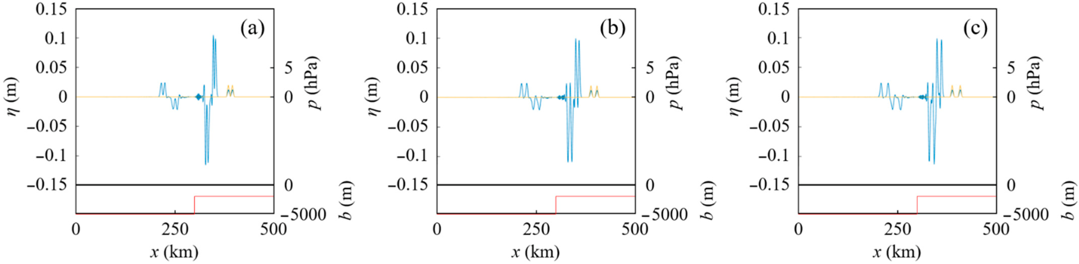
In Case C, two atmospheric pressure waves W1 and W2, as illustrated in Figure 1, traveled over the water on a stepped seabed, as depicted in Figure 2a. The conditions of Case C are described in Table 1. Figure 5 presents the water surface profiles at t = 1400 s in Case C, in which the interval of the atmospheric pressure waves, δ, is 0 km, 5 km, and 10 km.
In Figure 5, the lowest water level appears in the third trough below the still-water level when δ is 0 km, whereas in the second trough it appears below the still-water level when δ is 10 km. This indicates that the change in the water surface profile of each tsunami crossing an abrupt change in water depth depends on the interval or period of the atmospheric pressure waves. The reason for this is that the wave profile of a tsunami propagating as a free wave in shallower water depends on the water surface profile when the atmospheric pressure waves related to the tsunami travel over the abrupt change in water depth. The water surface profile due to the previous atmospheric pressure waves as the succeeding atmospheric pressure wave travels over the abrupt change in water depth depends on the intervals of these atmospheric pressure waves.
4.1.2. Effect of the Phase of a Tsunami-Generation Process Due to an Atmospheric Pressure Wave Train on the Resultant Tsunamis over a Stepped Seabed
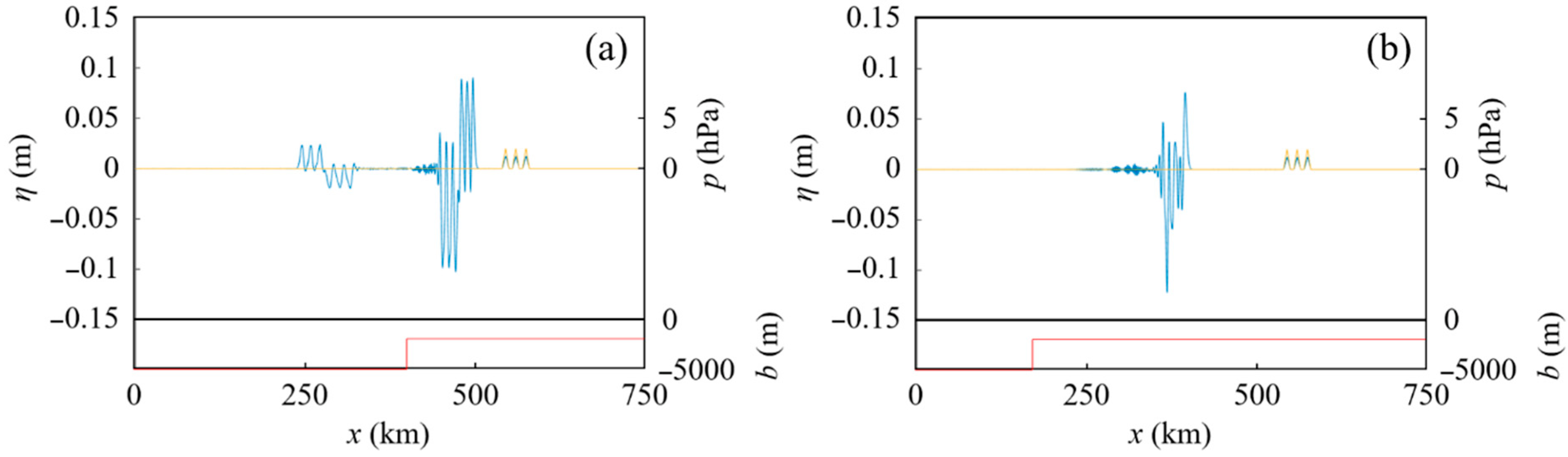
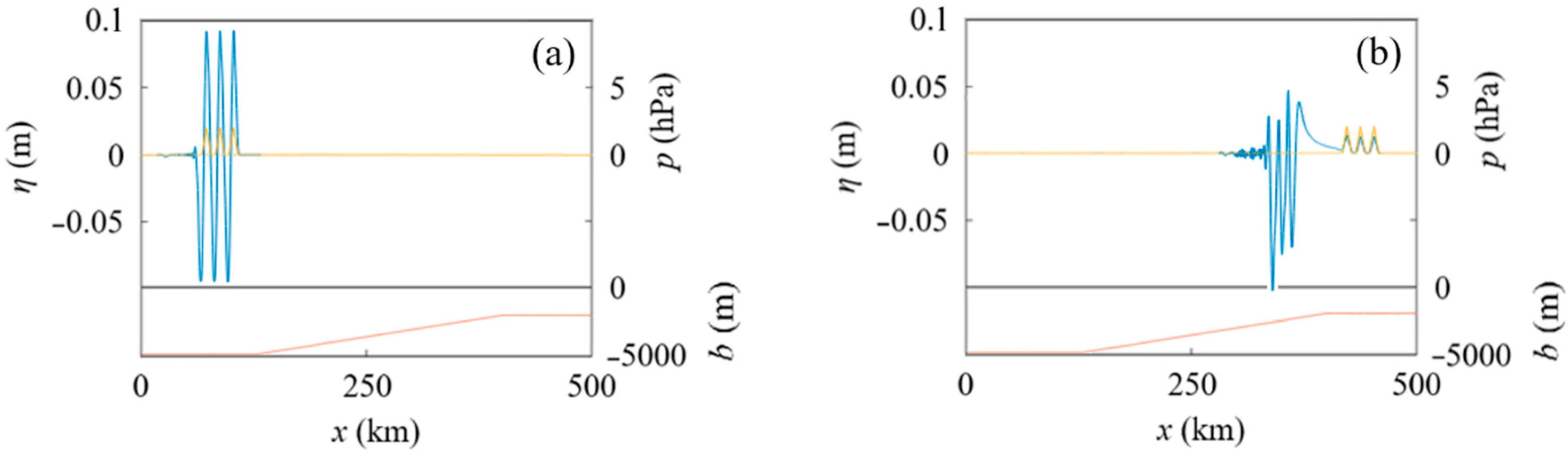
In Case D, three atmospheric pressure waves W1, W2, and W3, as illustrated in Figure 1, traveled over water on a stepped seabed, as depicted in Figure 2a, in which the still-water depth in the shallower area, hon, was 2000 m. The conditions of Case D are described in Table 1. Figure 6a,b depict the water surface profiles at t = 2100 s in Case D, in which the offshore end of the shallower area was located at xon = 400 km and 170 km, respectively.
The waveforms of the tsunamis propagating as free waves differ greatly between Figure 6a,b. In the former, all of the atmospheric pressure waves crossed over the abrupt change in water depth after W3 passed the troughs created by W1 and W2. Conversely, in the latter, W2 and W3 crossed over the abrupt change in water depth while passing the troughs generated by the previous atmospheric pressure waves. Thus, when tsunamis enter an area with a different still-water depth during their generation process due to an atmospheric pressure wave train, the water surface profile of the tsunamis will differ depending on the phase of the process.
4.1.3. Effect of the Difference between Two Water Depths over a Stepped Seabed on Tsunamis Generated by an Atmospheric Pressure Wave Train
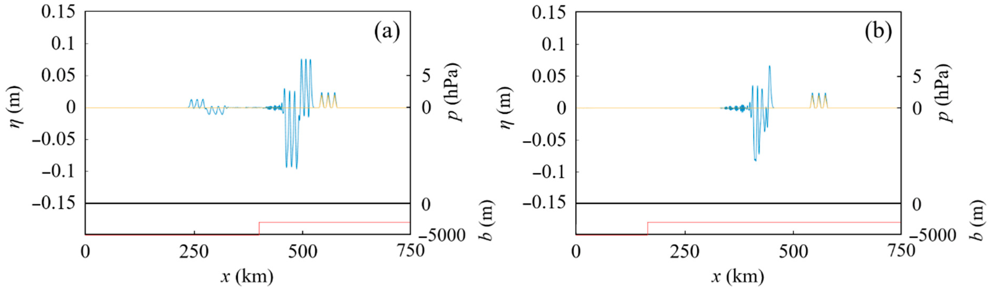
In Case E, three atmospheric pressure waves W1, W2, and W3, as illustrated in Figure 1, traveled over a water on a stepped seabed, as depicted in Figure 2a, in which the still-water depth in the shallower area, hon, was 3000 m. The conditions of Case E are described in Table 1. Figure 7a,b depict the water surface profiles at t = 2100 s in Case E, in which the offshore end of the shallower area was located at xon = 400 km and 170 km, respectively.
We compare Figure 6a with Figure 7a, in which the still-water depth in the shallower area, hon, is larger. In both cases, the first, second, and third tsunamis are forced waves following the atmospheric pressure waves. The maximum water levels in these three tsunamis are 0.012 m and 0.023 m in Figure 6a and Figure 7a, respectively. Conversely, the subsequent 4th, 5th, and 6th tsunamis are free waves. The maximum water levels in these tsunamis are 0.091 m and 0.077 m in Figure 6a and Figure 7a, respectively. Comparing the corresponding waves, the tsunami heights of the 1st, 2nd, and 3rd tsunamis in Figure 7a are higher than those in Figure 6a, whereas the tsunami heights of the 4th, 5th, and 6th waves in Figure 7a are lower than those in Figure 6a. The reason for this is that the Proudman resonance in the shallower water was more effective in the case of Figure 7. When the free 4th, 5th, and 6th tsunamis were left behind by the forced 1st, 2nd, and 3rd tsunamis, the decrease in the height of the 4th, 5th, and 6th tsunamis was greater in the case of Figure 7a.
It should be noted that the difference in the lowest water levels of the 8th, 9th, and 10th tsunami troughs between Figure 6a and Figure 7a is not as large as the tsunami height difference of the 4th, 5th, and 6th tsunamis between the same figures.
Furthermore, comparing Figure 7b with Figure 6b, as well as Figure 6a and Figure 7a, the waveforms of the tsunamis propagating as free waves are different. Figure 7b does not just indicate waveforms separated back and forth compared to Figure 6b. While an atmospheric pressure wave Wa passes existing free water waves generated by its previous atmospheric pressure waves, the crest and trough generated by Wa overlap with the existing free water waves, so the water level fluctuates, resulting in vibration or beating under an atmospheric pressure wave train. After Wa has passed all of the existing free water waves, a forced water wave with a steady wave profile travels following Wa if the still-water depth is uniform. Thus, the waveform of tsunamis during a generation process due to an atmospheric pressure wave train can differ when the tsunamis propagate over an abrupt change in water depth, upon which the effect of the atmospheric pressure wave train on the tsunamis suddenly changes based on the difference in water depth.
4.2. Tsunamis Generated by an Atmospheric Pressure Wave Train over a Sloping Seabed
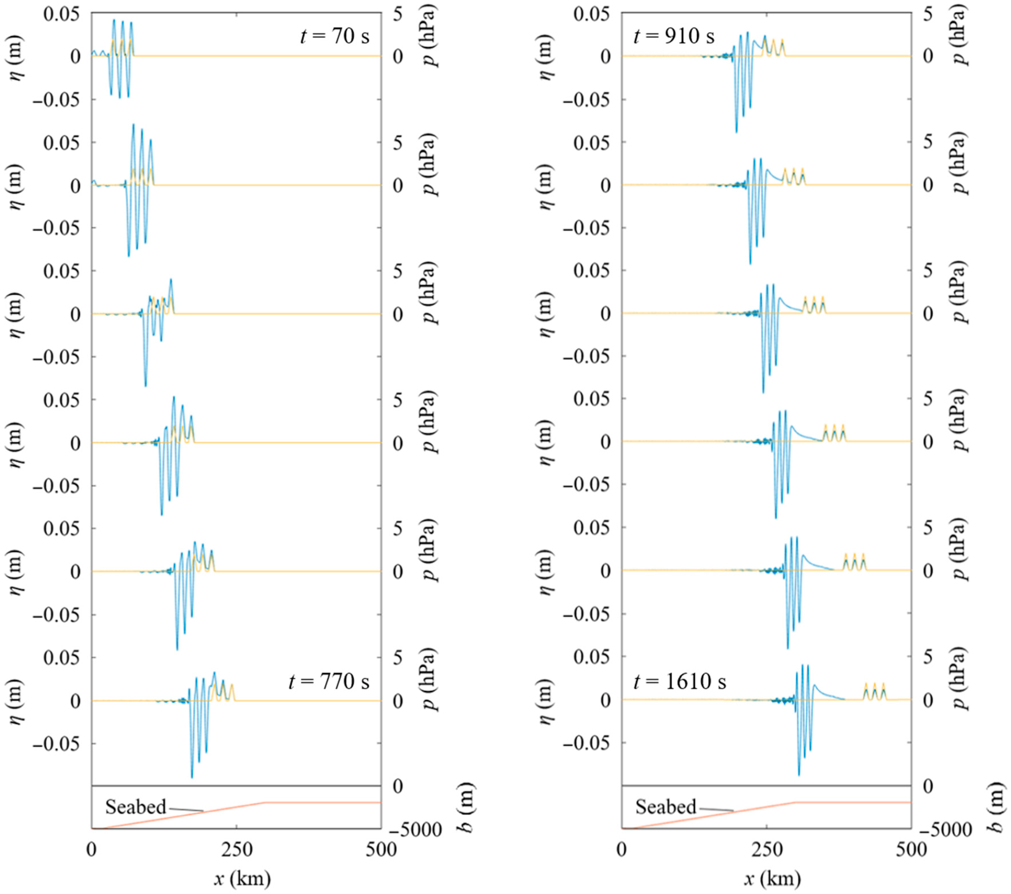
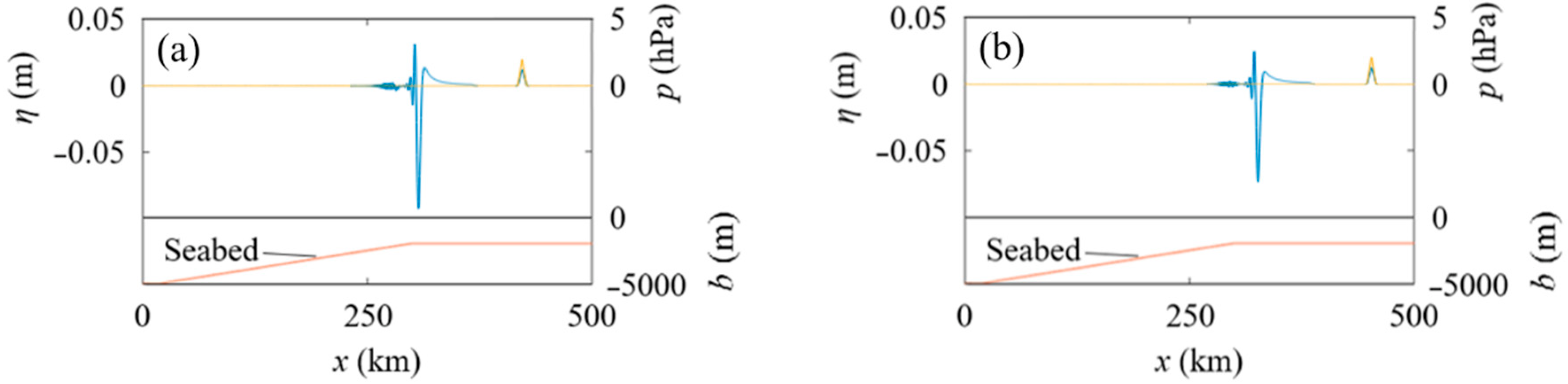
We consider an atmospheric pressure wave train that generates tsunamis over a sloping seabed in Case F. The seabed topography included a uniform slope, as depicted in Figure 2b, in which there was a slope with a constant gradient of β = 1.07 × 10⁻² at 20 km ≤ x ≤ 300 km. The atmospheric pressure waves were W1, W2, and W3, as illustrated in Figure 1. The conditions of Case F are described in Table 1. Figure 8 presents the time variation of the water surface profile in Case F.
In the figure on the left, the atmospheric pressure waves pass the existing free water waves generated by the previous atmospheric pressure waves, so the water surface profile indicates beating. Conversely, in the figure on the right, after all of the atmospheric pressure waves have passed the free waves, the water surface profile is relatively steady.
For comparison, in Case G, the same atmospheric pressure wave W1 as that in Case F existed and traveled at x ≤ 500 km over a flat seabed. The conditions of Case G are described in Table 1. The water surface profiles at t = 2100 s in Case G are depicted in Figure 9a–c, where the still-water depths are 5000 m, 3500 m, and 2000 m, respectively.
Compared to the approximately symmetrical crests and troughs in Figure 9, in Figure 8, the amplification of the tsunami crests propagating as free waves is controlled by leaving the forced waves following the atmospheric pressure waves, whereas the amplitudes of the free troughs are much larger than those of the free crests. The maximum water level of the 1st crest in Figure 9b is 0.047 m, while that of the 3rd free crest at t = 1610 s in Figure 8 is 0.043 m, where the uniform still-water depth in Figure 9b is the average on the slope in Figure 8. It should be noted that although these values are not so different, the value in Figure 8 was obtained through shallowing over the slope.
In Case H, one of the atmospheric pressure waves in Case F—i.e., W1 or W3—traveled over the same seabed as in Case F. The conditions of Case H are described in Table 1. The water surface profiles in Case H are depicted in Figure 10, for different locations of the onshore end of an atmospheric pressure wave W1 at t = 0 s, namely, x1.
Regarding the maximum water level of each wave at t = 1610 s, i.e., Hmax, the Hmax of the 1st free tsunami crest is 0.010 m in Figure 10b and 0.018 m in Figure 8, so the Hmax of the 1st free tsunami crest was amplified by being passed by two subsequent atmospheric pressure waves, as indicated in Figure 4, in which the existing tsunami TLamb was amplified by the passing atmospheric pressure waves.
Conversely, regarding the lowest water level of each wave at t = 1610 s, i.e., Hmin, the Hmin of the first trough is −0.091 m in Figure 10a and −0.075 m in Figure 10b, whereas in Figure 8, the Hmin of the 3rd and 1st free troughs is −0.086 m and −0.058 m, respectively. The differences between the corresponding waves were 0.091 m − 0.086 m = 0.005 m and 0.075 m − 0.058 m = 0.017 m, so the amplitude of the 1st free trough was more decreased than that of the 3rd free trough because of being passed by the atmospheric pressure waves.
It should be noted that when the atmospheric pressure is negative, the water surface profiles are approximately upside down from the above cases. When an atmospheric pressure wave profile is an inverted isosceles triangle with a minimum pressure of −2 hPa and the other conditions are the same as those in Figure 10b, the maximum water level of the first free crest was 0.073 m and the minimum water level of the first free trough was −0.010 m at t = 1610 s.
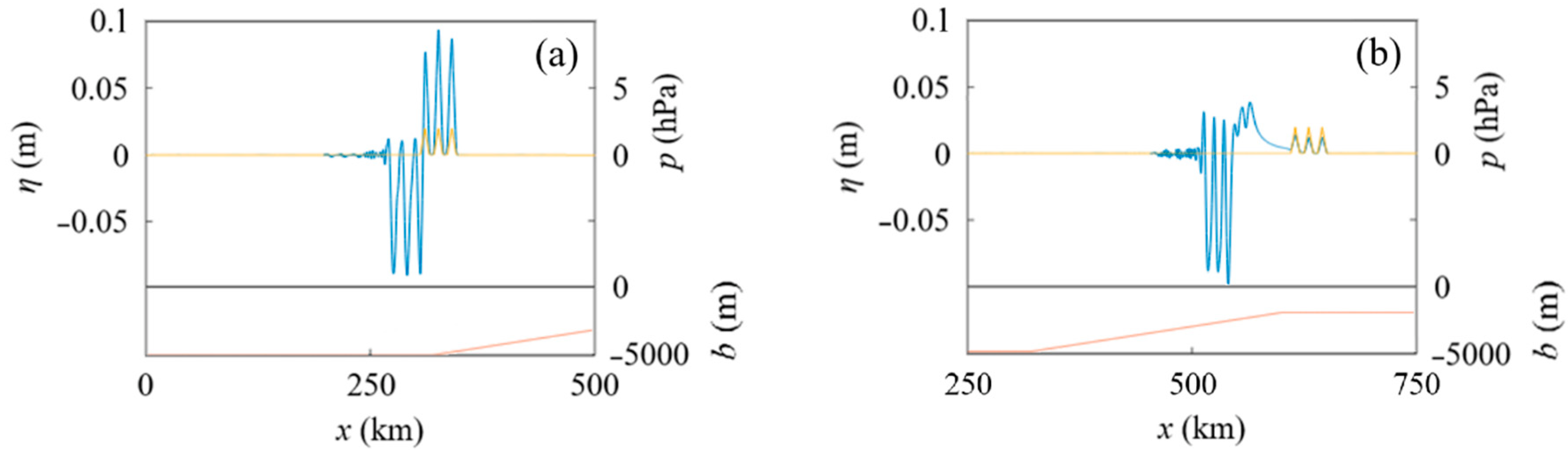
Furthermore, the lowest water level of the 1st, 2nd, and 3rd free tsunami troughs is denoted by ζ1, ζ2, and ζ3, respectively. In Figure 8, for Case F, the lowest water levels of these troughs are different, with a relationship of ζ1 > ζ2 > ζ3. To investigate this relationship, the same atmospheric pressure waves W1, W2, and W3 as those in Case F traveled over a slope in Case I, in which the slope gradient was the same as that in Case F but the locations of the offshore end of the slope, i.e., xslope, were different. Figure 11 and Figure 12 present the water surface profiles in Case I.
As indicated in Figure 11a, the atmospheric pressure wave train started traveling over the offshore flat seabed, and the relationship between the lowest water levels of the free troughs was ζ1 > ζ2 > ζ3, as shown in Figure 11b, as at t = 1610 s in Figure 8. Conversely, in Figure 12b, the relationship is ζ1 < ζ2 ≃ ζ3, which is different from that in Figure 11b. As indicated in Figure 12a, although the atmospheric pressure wave train also started traveling over the offshore flat seabed—as in the case of Figure 11—the atmospheric pressure wave train passed all of the free tsunami troughs generated by the previous atmospheric pressure waves over the offshore flat seabed. In the case of Figure 11, the atmospheric pressure waves approached the slope in the tsunami-generation process, so the water surface profile of the free tsunamis depended on the phase of the tsunami-generation process over the starting location of the slope. In the case of Figure 8, the atmospheric pressure wave train started traveling over the slope, and the tsunami-generation process was carried out over the slope, as in the case of Figure 11. Thus, both the waveforms and the amplitudes of tsunamis caused by an atmospheric pressure wave train depend on the phase of the tsunami-generation process over changes in water depth.
5. Brief Discussion on a Tide-Gauge Record
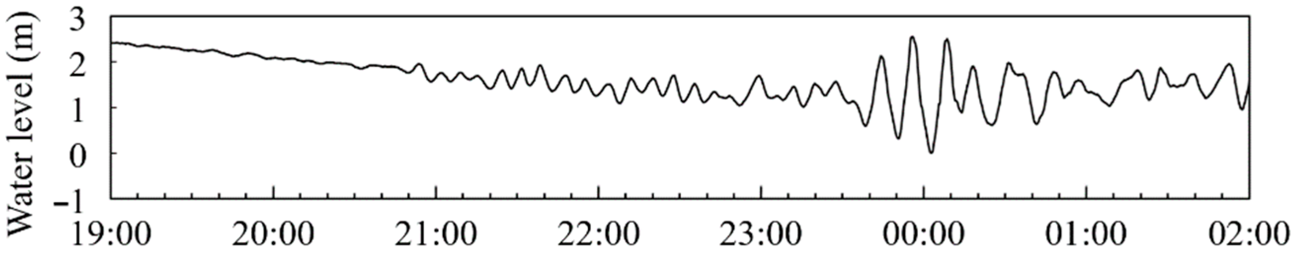
Regarding the 2022 Hunga Tonga–Hunga Ha’apai volcanic eruption tsunamis, the tide-gauge record obtained by the Japan Meteorological Agency at Amami, Kagoshima, Japan from 19:00 on 15 January to 02:00 on 16 January 2022 (JST) is depicted in Figure 13. In the present paper, the time is described using Japan Standard Time (JST), which is Coordinated Universal Time (UTC) + 9 h. At Amami, anomalous tide-level fluctuations with a period of approximately 7.5 min started around 20:50 on 15 January.
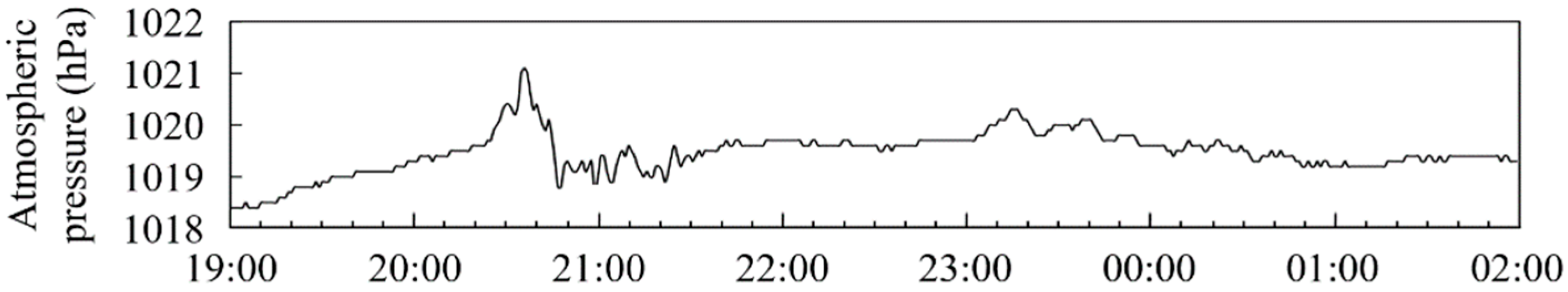
Moreover, Figure 14 depicts the atmospheric pressure obtained by Weathernews at Amami in the same term. At Amami, the large atmospheric pressure fluctuations started around 20:25 on 15 January.
Therefore, the anomalous tide-level fluctuations described above, which started approximately 25 min after the arrival time of the atmospheric pressure wave, were due to the tsunamis following the atmospheric pressure waves. Conversely, the tsunamis generated at the eruption site were predicted to reach Amami at around 00:30 on January 16 [1].
Thereafter, as indicated in Figure 13, remarkable tide-level fluctuations with a period of approximately 12 min started around 23:35 on 15 January, and the total amplitude exceeded 2.5 m. In the tide-level fluctuations from 23:35 on 15 January to 00:10 on 16 January, the lowest water levels of the 1st, 2nd, and 3rd troughs—i.e., z1, z2, and z3, respectively—indicate the relationship z1 > z2 > z3, which resembles the above-described relationship ζ1 > ζ2 > ζ3 of the free troughs depicted in Figure 8 for the model case with a sloping seabed. This suggests that the tsunami-generation processes were carried out over a slope or intermittent changes in water depth. However, such a relationship may also appear when a seiche gradually increases, and future analyses with both actual barometric records and in-depth bathymetry data are necessary to quantitatively explain the tide-level fluctuations at Amami, considering the phases of the tsunami-generation processes.
In Figure 13, the difference between the start time of the anomalous tide-level fluctuations, i.e., 20:50, and the start time of the remarkable tide-level fluctuations, i.e., 23:35, at Amami is 2 h 45 min. Assuming that the eruption time was 13:00, the traveling time tL of the atmospheric Lamb wave to Amami was 7 h 50 min, and the arrival time tt of the remarkable tsunamis at Amami was 10 h 35 min after the eruption. It is assumed that the tsunamis generated by atmospheric pressure waves started propagation at a location as free waves with a phase velocity lower than that of the atmospheric pressure waves. When the average water depth is D and the phase velocity of the tsunamis is , the distance ΔL between this location and Amami can be calculated as follows:
where v is the traveling velocity of the atmospheric pressure waves from the eruption site and vL is that of the atmospheric Lamb wave. We assume that vL is 310 m/s, and when the average water depth considering a shelf is 2000 m, the tsunami phase velocity is approximately 140 m/s. Thus ΔL is approximately 2500 km when v is 310 m/s, whereas ΔL is approximately 1000 km when v is 250 m/s, based on Equation (4). The tsunamis away from the action of the atmospheric pressure waves at a location ΔL offshore from the tide station could be the external force behind the remarkable tide-level fluctuations that started around 23:35.
When ΔL was 2500 km, the tsunamis were generated by the atmospheric Lamb wave at trenches with a large water depth, including the Mariana Trench, and then amplified by the subsequent atmospheric pressure waves at nearer and shallower areas, resulting in the remarkable tide-level fluctuations at Amami.
Conversely, when ΔL is 1000 km, in such a location, there are no deep areas such as trenches, at which the atmospheric Lamb wave is effective for tsunami generation. Therefore, the subsequent atmospheric pressure waves could generate and amplify the tsunamis over topographic changes, leading to the remarkable tide-level fluctuations. In this case, the tsunamis generated by the atmospheric Lamb wave in deeper waters, such as the Mariana Trench, arrived at Amami after 23:35.
The tsunamis generated and amplified through the Proudman resonance at these locations could be further amplified by shallowing and seiche. Future work is required to investigate the tsunami-generation mechanisms in various volcanic eruptions, comparing observed data with the corresponding numerical results using model and actual atmospheric pressure waves and bathymetries, in consideration of both the nonlinearity and dispersion of waves.
6. Conclusions
As a fundamental study on the processes of tsunami generation and amplification by an atmospheric pressure wave train, numerical simulations were generated using a nonlinear shallow-water model of velocity potential. In the computation, the steady atmospheric pressure wave trains were advanced at a constant velocity over an abrupt change in water depth or a uniform slope.
When the atmospheric pressure wave caught up with the existing tsunami traveling as a free wave over the abrupt change in water depth, the amplified tsunami propagated in the shallower area. The existing tsunami traveling as a free wave over the sloping seabed was also amplified by the passing atmospheric pressure waves, where the increase in tsunami height due to the increase in the number of atmospheric pressure waves decreased, as the number of atmospheric pressure waves was increased.
When the atmospheric pressure waves crossed over the abrupt change in water depth, the water surface profiles of tsunamis in the shallower water depended on both the interval of the atmospheric pressure waves and the phase of the tsunami-generation process over the change in water depth. Moreover, when the atmospheric pressure waves traveled over the abrupt change in water depth, the tsunami amplitude in the shallower area increased, as the water depth of the shallower area was decreased and the Proudman resonance was further reduced.
When the atmospheric pressure wave train with positive pressure traveled over the sloping seabed, the amplification of the crests of the tsunamis propagating as free waves was controlled by leaving the forced water waves following the atmospheric pressure waves. Conversely, the amplitudes of the tsunami troughs propagating as free waves were increased.
Funding
This work was supported by JSPS KAKENHI Grants, the grant numbers of which were JP17K06585 and JP21K21353.
Acknowledgments
Sincere gratitude is extended to the anonymous reviewers for their valuable comments that improved the paper. The author would like to appreciate Mozer, A. and the editorial team. The discussion with Yamashita, K. of Nuclear Regulation Agency was informative, and he assisted in the calculations using the Boussinesq-type model for the model validation. Tide-level and atmospheric pressure data provided by the Japan Meteorological Agency and Weathernews, respectively, were used to create the figures in Section 5.
Conflicts of Interest
The author declares no conflict of interest.
Appendix A
In Section 2, the following Boussinesq-type equations considering both the weak nonlinearity and weak dispersion of waves were also applied:
where η(x, t), Q(x, t), h(x, t), and p(x, t) are the water surface displacement, flow rate in the x-axis direction, still-water depth, and pressure on the water surface, respectively. Equations (A1) and (A2) were proposed and applied in [25], with reference to the dispersion term of [26], and also utilized by [27] to calculate transoceanic tsunamis. In Section 2, these equations were transformed to finite difference equations, as in [27], and solved numerically, where the grid size Δx was 100 m and the time interval Δt was 0.05 s.
References
- Japan Meteorological Agency Earthquake Volcano Department. On the tide level change due to the large eruption of Hunga Tonga-Hunga Ha’apai volcano near the Tonga Islands around 13:00 on January 15, 2022. Jpn. Meteorol. Agency Press Release 2022, 11, 23. Available online: https://www.jma.go.jp/jma/press/2201/16a/kaisetsu202201160200.pdf (accessed on 10 May 2022). (In Japanese).
- Proudman, J. The effects on the sea of changes in atmospheric pressure. Geophys. J. Int. 1929, 2, 197–209. [Google Scholar] [CrossRef]
- Kakinuma, T. Long-wave generation due to atmospheric pressure variation and harbor oscillation in harbors of various shapes and countermeasures against meteotsunamis. In Natural Hazards—Risk, Exposure, Response, and Resilience; Tiefenbacher, J., Ed.; InTech: London, UK, 2019; pp. 81–109. [Google Scholar] [CrossRef] [Green Version]
- Verbeek, R.D.M. Krakatau; Government Press: Batavia, IL, USA, 1885; 495p. [Google Scholar]
- Symons, G.J. (Ed.) The Eruption of Krakatoa, and Subsequent Phenomena, Report of the Krakatoa Committee of the Royal Society; Trübner and Co.: London, UK, 1888; 494p. [Google Scholar]
- Imamura, A. Observation of Krakatau explosion tsunami in Japan: Earthquake Chat (10). Earthquake 1934, 1, 158–160. (In Japanese) [Google Scholar]
- Harkrider, D.; Press, F. The Krakatoa air-sea waves: An example of pulse propagation in coupled systems. Geophys. J. R. Astron. Soc. 1967, 13, 149–159. [Google Scholar] [CrossRef] [Green Version]
- Garrett, C.J.R. A theory of the Krakatoa tide gauge disturbances. Tellus 1970, 22, 43–52. [Google Scholar] [CrossRef]
- Yokoyama, I. A geophysical interpretation of the 1883 Krakatau eruption. J. Volcanol. Geotherm. Res. 1981, 9, 359–378. [Google Scholar] [CrossRef]
- Yokoyama, I. A scenario of the 1883 Krakatau tsunami. J. Volcanol. Geotherm. Res. 1987, 34, 123–132. [Google Scholar] [CrossRef]
- Pelinovsky, E.; Choi, B.H.; Stromkov, A.; Didenkulova, I.; Kim, H.-S. Analysis of tide-gauge records of the 1883 Krakatau Tsunami. In Tsunamis: Case Studies and Recent Developments, Advances in Natural and Technological Hazards Research, 23; Satake, K., Ed.; Springer: Dordrecht, The Netherlands, 2005; pp. 57–77. [Google Scholar] [CrossRef]
- Soloviev, S.L. Basic data of tsunamis in the Pacific coast of USSR, 1937–1976. In A Study of Tsunamis in the Open Sea; Academii Nauk: Moscow, Russia, 1978; pp. 61–136. (In Russian) [Google Scholar]
- Kobayashi, T.; Kakinuma, T. Tsunamis propagated by airwaves generated by explosive volcanic eruptions: The 1883 Krakatau and the 1956 Bezymianny eruptions. In Proceedings of the International Meeting on Eruptive History and Informatics 2021-2, Fukuoka, Japan, 5–6 March 2022; pp. 93–105. (In Japanese). [Google Scholar]
- Sekizawa, S.; Kohyama, T. Meteotsunami observed in Japan following the Hunga Tonga eruption in 2022 investigated using a one-dimensional shallow-water model. SOLA 2022. preprint. [Google Scholar] [CrossRef]
- Tanioka, Y.; Yamanaka, Y.; Nakagaki, T. Characteristics of the deep sea tsunami excited offshore Japan due to the air wave from the 2022 Tonga eruption. Earth Planets Space 2022, 74, 61. [Google Scholar] [CrossRef]
- Kubota, T.; Saito, T.; Nishida, K. Global fast-traveling tsunamis driven by atmospheric Lamb waves on the 2022 Tonga eruption. Science 2022, eabo4364. [Google Scholar] [CrossRef] [PubMed]
- Pakoksung, K.; Suppasri, A.; Imamura, F. Tsunami Simulation (without Air-Sea Waves) on the 2022/01/15 Hunga Tonga-Hunga Ha’apai Submarine Volcanic Explosion. 2022. Available online: https://irides.tohoku.ac.jp/research/prompt_investigation/2022_tonga-vol-tsunami.html (accessed on 10 May 2022).
- Ramírez-Herrera, M.T.; Coca, O.; Vargas-Espinosa, V. Tsunami effects on the Coast of Mexico by the Hunga Tonga-Hunga Ha’apai volcano eruption, Tonga. Pure Appl. Geophys. 2022, 179, 1117–1137. [Google Scholar] [CrossRef] [PubMed]
- Carvajal, M.; Sepúlveda, I.; Gubler, A.; Garreaud, R. Worldwide signature of the 2022 Tonga volcanic tsunami. Geophys. Res. Lett. 2022, 49, e2022GL098153. [Google Scholar] [CrossRef]
- Hibiya, T.; Kajiura, K. Origin of the Abiki phenomenon (a kind of seiche) in Nagasaki Bay. J. Oceanogr. Soc. Jpn. 1982, 38, 172–182. [Google Scholar] [CrossRef]
- Vilibić, I.; Monserrat, S.; Rabinovich, A.; Mihanović, H. Numerical modelling of the destructive meteotsunami of 15 June, 2006 on the coast of the Balearic Islands. Pure Appl. Geophys. 2008, 165, 2169–2195. [Google Scholar] [CrossRef]
- Asano, T.; Yamashiro, T.; Nishimura, N. Field observations of meteotsunami locally called “abiki” in Urauchi Bay, Kami-Koshiki Island, Japan. Nat. Hazards 2012, 64, 1685–1706. [Google Scholar] [CrossRef]
- Bailey, K.E.; DiVeglio, C.; Welty, A. An examination of the June 2013 East Coast meteotsunami captured by NOAA observing systems. NOAA Tech. Rep. NOS CO-OPS 2014, 79, 42. Available online: https://repository.library.noaa.gov/view/noaa/14435 (accessed on 10 May 2022).
- Tanaka, K.; Ito, D. Multiscale meteorological systems resulted in meteorological tsunamis. In Tsunami; Mokhtari, M., Ed.; InTech: Rijeka, Balkans, 2016; pp. 13–33. [Google Scholar] [CrossRef] [Green Version]
- Iwase, H.; Mikami, T.; Goto, C. Practical tsunami numerical simulation model by use of non-linear dispersive long wave theory. J. JSCE 1998, 1998, 119–124. [Google Scholar] [CrossRef] [Green Version]
- Peregrine, D.H. Long waves on a beach. J. Fluid Mech. 1967, 27, 815–827. [Google Scholar] [CrossRef]
- Baba, T.; Allgeyer, S.; Hossen, J.; Cummins, P.R.; Tsushima, H.; Imai, K.; Yamashita, K.; Kato, T. Accurate numerical simulation of the far-field tsunami caused by the 2011 Tohoku earthquake, including the effects of Boussinesq dispersion, seawater density stratification, elastic loading, and gravitational potential change. Ocean Model. 2017, 111, 46–54. [Google Scholar] [CrossRef]
Figure 1.
Wave profiles of atmospheric pressure waves traveling in the positive direction of the x-axis at the initial time, i.e., t = 0 s. The length and maximum pressure of the waves are denoted by λ and pmax, respectively, and the interval between the waves is δ. The location of the onshore end of the nth wave Wn is xn at t = 0 s.

Figure 2.
Two types of seabed topography, where hoff = 5000 m: (a) Stepped seabed topography. (b) Partially sloping topography.
Figure 2.
Two types of seabed topography, where hoff = 5000 m: (a) Stepped seabed topography. (b) Partially sloping topography.

Figure 3.
Water surface profiles at t = 1050 s in Case A, in which x1 = 55 km in Figure 1; hon = 2000 m and xon = 170 km in Figure 2a. The blue, orange, and red lines indicate the water surface displacement η, atmospheric pressure p, and seabed position b, respectively. (a) The existing tsunami TLamb propagated without the atmospheric pressure wave W1. (b) Tsunamis were generated by W1 without TLamb. (c) TLamb was amplified by W1.

Figure 4.
Water surface profiles at t = 2380 s in Case B, in which x1 = 55 km and δ = 5 km in Figure 1; hon = 2000 m, xslope = 20 km, xon = 500 km, and the slope gradient β = 6.25 × 10⁻³ in Figure 2b. The blue, orange, and red lines indicate the water surface displacement η, atmospheric pressure p, and seabed position b, respectively. (a) The existing tsunami TLamb propagated with no atmospheric pressure wave. (b) TLamb was amplified by W1. (c) TLamb was amplified by W1 and W2. (d) TLamb was amplified by W1, W2, and W3. (e) TLamb was amplified by W1, W2, W3, and W4.

Figure 5.
Water surface profiles at t = 1400 s for different intervals of the atmospheric pressure waves, δ, in Case C, in which x2 = 40 km in Figure 1; hon = 2000 m and xon = 300 km in Figure 2a. The blue, orange, and red lines indicate the water surface displacement η, atmospheric pressure p, and seabed position b, respectively. (a) δ = 0 km, (b) δ = 5 km, and (c) δ = 10 km in Figure 1.

Figure 6.
Water surface profiles at t = 2100 s for different offshore end positions of the shallower area, xon, in Case D, in which x1 = 55 km and δ = 5 km in Figure 1; hon = 2000 m in Figure 2a. The blue, orange, and red lines indicate the water surface displacement η, atmospheric pressure p, and seabed position b, respectively. (a) xon = 400 km and (b) xon = 170 km in Figure 2a.

Figure 7.
Water surface profiles at t = 2100 s for different offshore end positions of the shallower area, xon, in Case E, in which x1 = 55 km and δ = 5 km in Figure 1; hon = 3000 m in Figure 2a. The blue, orange, and red lines indicate the water surface displacement η, atmospheric pressure p, and seabed position b, respectively. (a) xon = 400 km and (b) xon = 170 km in Figure 2a.

Figure 8.
Time variation of the water surface profile every 140 s in 70 s ≤ t ≤ 1610 s in Case F, in which x1 = 55 km and δ = 5 km in Figure 1; hon = 2000 m, xslope = 20 km, xon = 300 km, and the slope gradient β = 1.07 × 10⁻² in Figure 2b. The blue, orange, and red lines indicate the water surface displacement η, atmospheric pressure p, and seabed position b, respectively.

Figure 9.
Water surface profiles at t = 2100 s for different still-water depths h in Case G, in which x1 = 55 km in Figure 1. The blue, orange, and red lines indicate the water surface displacement η, atmospheric pressure p, and seabed position b, respectively. (a) h = 5000 m. (b) h = 3500 m. (c) h = 2000 m.

Figure 10.
Water surface profiles at t = 1610 s for different values of x1 in Case H, in which hon = 2000 m, xslope = 20 km, xon = 300 km, and the slope gradient β = 1.07 × 10⁻² in Figure 2b. The blue, orange, and red lines indicate the water surface displacement η, atmospheric pressure p, and seabed position b, respectively. (a) x1 = 25 km and (b) x1 = 55 km in Figure 1.

Figure 11.
Water surface profiles in Case I, where x1 = 55 km and δ = 5 km in Figure 1; hon = 2000 m, xslope = 120 km, xon = 400 km, and the slope gradient β = 1.07 × 10⁻² in Figure 2b. The blue, orange, and red lines indicate the water surface displacement η, atmospheric pressure p, and seabed position b, respectively. (a) t = 210 s. (b) t = 1610 s.

Figure 12.
Water surface profiles in Case I, where x1 = 55 km and δ = 5 km in Figure 1; hon = 2000 m, xslope = 320 km, xon = 600 km, and the slope gradient β = 1.07 × 10⁻² in Figure 2b. The blue, orange, and red lines indicate the water surface displacement η, atmospheric pressure p, and seabed position b, respectively. (a) t = 1190 s. (b) t = 2380 s.

Figure 13.
The tide-gauge record obtained at Kominato, Amami, Kagoshima, Japan from 19:00 on 15 January to 02:00 on 16 January 2022 (JST). Information from the Japan Meteorological Agency was used to create the figure.
Figure 13.
The tide-gauge record obtained at Kominato, Amami, Kagoshima, Japan from 19:00 on 15 January to 02:00 on 16 January 2022 (JST). Information from the Japan Meteorological Agency was used to create the figure.

Figure 14.
Atmospheric pressure observed every minute at Uken on Amami Oshima Island, Kagoshima, Japan, using the IoT sensor “Soratena” produced by Weathernews, from 19:00 on 15 January to 02:00 on 16 January 2022 (JST).
Figure 14.
Atmospheric pressure observed every minute at Uken on Amami Oshima Island, Kagoshima, Japan, using the IoT sensor “Soratena” produced by Weathernews, from 19:00 on 15 January to 02:00 on 16 January 2022 (JST).


Table 1.
Calculation conditions. The traveling velocity vp of every atmospheric pressure wave was 250 m/s. The uniform still-water depth in the offshore deepest area, hoff, was 5000 m. The slope gradient is β.
Table 1.
Calculation conditions. The traveling velocity vp of every atmospheric pressure wave was 250 m/s. The uniform still-water depth in the offshore deepest area, hoff, was 5000 m. The slope gradient is β.
| Case | Existing Tsunami TLamb | Number of Atmospheric Pressure Waves | Interval of Atmospheric Pressure Waves, δ | Initial Position of the nth Atmospheric Pressure Wave, xn | Seabed Topography | Still-Water Depth in the Onshore Shallowest Area, hon | Offshore End Location of the Onshore Shallowest Area, xon | Offshore End Location of the Slope, xslope |
|---|---|---|---|---|---|---|---|---|
| A | Presence | 0 | — | x1 = 55 km | Stepped | 2000 m | 170 km | — |
| 1 | ||||||||
| Absence | 1 | |||||||
| B | Presence | 0 | — | x1 = 55 km | Partially Sloping β = 6.25 × 10⁻³ | 2000 m | 500 km | 20 km |
| 1 | ||||||||
| 2 | 5 km | |||||||
| 3 | ||||||||
| 4 | ||||||||
| C | Absence | 2 | 0 km 5 km 10 km | x2 = 40 km | Stepped | 2000 m | 300 km | — |
| D | Absence | 3 | 5 km | x1 = 55 km | Stepped | 2000 m | 170 km 400 km | — |
| E | Absence | 3 | 5 km | x1 = 55 km | Stepped | 3000 m | 170 km 400 km | — |
| F | Absence | 3 | 5 km | x1 = 55 km | Partially Sloping β = 1.07 × 10⁻² | 2000 m | 300 km | 20 km |
| G | Absence | 1 | — | x1 = 55 km | Flat | 2000 m 3500 m 5000 m | 0 km | — |
| H | Absence | 1 | — | x1 = 25 km, x1 = 55 km | Partially Sloping β = 1.07 × 10⁻² | 2000 m | 300 km | 20 km |
| I | Absence | 3 | 5 km | x1 = 55 km | Partially Sloping β = 1.07 × 10⁻² | 2000 m | 400 km | 120 km |
| 600 km | 320 km |
Publisher’s Note: MDPI stays neutral with regard to jurisdictional claims in published maps and institutional affiliations. |
© 2022 by the author. Licensee MDPI, Basel, Switzerland. This article is an open access article distributed under the terms and conditions of the Creative Commons Attribution (CC BY) license (https://creativecommons.org/licenses/by/4.0/).
Share and Cite
MDPI and ACS Style
Kakinuma, T. Tsunamis Generated and Amplified by Atmospheric Pressure Waves Due to an Eruption over Seabed Topography. Geosciences 2022, 12, 232. https://0-doi-org.brum.beds.ac.uk/10.3390/geosciences12060232
AMA Style
Kakinuma T. Tsunamis Generated and Amplified by Atmospheric Pressure Waves Due to an Eruption over Seabed Topography. Geosciences. 2022; 12(6):232. https://0-doi-org.brum.beds.ac.uk/10.3390/geosciences12060232
Chicago/Turabian StyleKakinuma, Taro. 2022. "Tsunamis Generated and Amplified by Atmospheric Pressure Waves Due to an Eruption over Seabed Topography" Geosciences 12, no. 6: 232. https://0-doi-org.brum.beds.ac.uk/10.3390/geosciences12060232
Note that from the first issue of 2016, this journal uses article numbers instead of page numbers. See further details here.