A Review of Advances in the Identification and Characterization of Groundwater Dependent Ecosystems Using Geospatial Technologies

Abstract

Groundwater Dependent Ecosystem (GDE) protection is increasingly being recognized as essential for the sustainable management and allocation of water resources. GDE services are crucial for human well-being and for a variety of flora and fauna. However, the conservation of GDEs is only possible if knowledge about their location and extent is available. Several studies have focused on the identification of GDEs at specific locations using ground-based measurements. However, recent progress in remote sensing technologies and their integration with Geographic Information Systems (GIS) has provided alternative ways to map GDEs at a much larger spatial extent. This paper presents a review of the geospatial methods that have been used to map and delineate GDEs at spatial different extents. Additionally, a summary of the satellite sensors useful for identification of GDEs and the integration of remote sensing data with ground-based measurements in the process of mapping GDEs is presented.

1. Introduction

Human well-being is largely dependent on ecosystems and the services they provide. Ecosystem change has been remarkable over the past 50 years, when human actions have changed the world’s ecosystems’ structures and functions more rapidly than in any other time in human history [1]. The anthropogenic effects associated with the degradation of ecosystems are closely linked to the increasing demands for resources such as water to support agriculture, industrial expansion, economic development, and population growth [2].

Groundwater use has greatly intensified in the past few decades and represents the greatest portion of modern increase in global water use. Currently, groundwater is the world’s most extracted raw material with withdrawal rates up to 982 km³/year [3]. There is a growing risk of depletion of groundwater resources in most parts of the world because, as surface water supplies are being exhausted and contaminated, and the feasibility to capture and store these resources has declined, groundwater has become the next-generation resource to meet future water needs. For instance, groundwater currently dominates surface water use for irrigation in many countries, such as Algeria, India, Iran, and Syria [4].

Groundwater is not an isolated resource and its allocation should be performed considering human requirements for freshwater in addition to the environmental problems associated with groundwater extraction and use such as declining quality of groundwater resources due to contamination by nutrients, salts, organic chemicals, and pathogens, along with the issue of sustainability of the source itself and the ecosystems that it supports. Even though groundwater is a renewable source, severe problems of groundwater quantity are related to the fact that the rate of replenishment is surpassed by the rate of groundwater pumping [5]. Where insufficient time is allowed for the aquifers to be replenished, results include reduced water supply, diminished surface water flows, economic losses, higher pumping costs, land subsidence, infrastructure damage, and negative impacts on ecosystems [6].

There has been increasing recognition of the ecological as well as economic importance of groundwater [4]. Several policies and regulations have been formulated with the purpose of protecting groundwater as a drinking water supply or other human uses [7]. However, significant efforts are still required to understand the relationship between groundwater and the ecosystems they support, as a key step in linking human and ecological water requirements. Groundwater plays a critical role in sustaining and maintaining the ecological integrity of several terrestrial, aquatic, and coastal ecosystems [8]. If groundwater allocation managers and groundwater policy and management systems are to adequately take into consideration ecosystems supported by groundwater, the first step is to identify the nature, extent, and degree of dependency of such ecosystems [9,10]. It is impossible to characterize the degree of groundwater reliance, and therefore the ecological response to change, without first understanding where the ecosystems occur.

2. Background

Many types of terrestrial vegetation and surface water systems (rivers, lakes, wetlands, and springs), together with the fauna they sustain, depend on groundwater. These are usually called Groundwater Dependent Ecosystems (GDEs). A GDE is a community of plants, animals, and microorganisms that relies partially or completely on the availability of groundwater to maintain its structure (the type and quantities of the different plants and animals that together form the community), and function (the ecosystem’s activities or behavior, such as plants taking up carbon through photosynthesis) [11]. A simple classification of GDEs was suggested [12]:

• Ecosystems dependent on the surface expression of groundwater: This category includes springs, “minerogenous” wetlands (wetlands supported by groundwater that has been in contact with mineral soils or bedrock), river baseflow systems, and some estuarine and near-shore marine ecosystems that depend on the discharge of groundwater.
• Ecosystems dependent on the subsurface expression of groundwater: This type includes terrestrial vegetation that uses shallow groundwater (phreatophytes). These plants access groundwater by extending their roots to the water table or to the capillary fringe right above it. The roots of phreatophytes extend up to 3 m to over 15 m below the land surface depending on the species [13,14].
• Aquifer and cave ecosystems: These include fractured rock, karstic, and alluvial aquifers, hyporheic zones of rivers and floodplains (saturated interstitial area beneath and alongside a stream bed where shallow groundwater and surface water mix), and stygofauna (organisms living in groundwater systems or aquifers).

GDEs are of crucial importance for a variety of ecological resources and the conservation of biodiversity. GDEs also play a crucial role in water quality of both surface waters and groundwater. For instance, micro-fauna present in groundwater supports its decontamination, maintaining the health of surface waters. GDEs also contribute to the prevention of soil erosion, serve as corridors for the migration of several species, have a great economic and aesthetic value in places with recreational purposes such as national parks and fisheries, and they also provide ecosystem services such as carbon capture and runoff interception [11,12].

Recently, the impact of anthropogenic climate change on groundwater and associated ecosystems has received significant attention [15,16,17,18,19,20,21] because aquifers and GDEs are increasingly threatened by local and regional anthropogenic alterations as well as climate change and variability. Alterations in the climate reflected in reduced precipitation and increased evapotranspiration have a detrimental effect on groundwater levels because of the reduction in groundwater recharge and increase in groundwater withdrawals to meet demands. A comprehensive summary of climate change impacts on GDEs is provided by [20]. This discussion is based on aspects that influence the biodiversity and functioning of GDEs, and it is complemented with identification of research gaps and sustainable groundwater management strategies.

The protection of GDEs for sustainable water management is extremely challenging because it requires the integration of environmental, economical, and socio-political spheres through the development of policies that effectively address the conservation of these ecosystems but still allow groundwater to be extracted at sufficient rates. Difficulties in protecting GDEs are the lack of understanding about the response trajectory of GDEs to groundwater over extraction and quantifying the volume of groundwater used by GDEs, in addition to the lack (or poor implementation) of policies for managing groundwater and conserving GDEs, which are usually a consequence of attempts to manage an issue (such as groundwater withdrawal) that is local or regional in nature, using national-level policies [22]. An additional major challenge to protecting GDEs is that knowledge about the locations where they occur is required. Even though this information might be available for specific locations, little or no information is available for over most large regions [23]. This knowledge gap is the major limitation in the process of informing water resource managers and decision makers of the amount of water required to sustain an ecosystem structure and function, and therefore in the establishment of the amount of water that can be appropriately allocated for social and economic purposes. Geospatial technologies, such as remote sensing and Geographic Information Systems (GIS), can play a key role in providing practical and economical means to study landscapes likely to contain GDEs, especially in large and remote areas.

This paper is a review of methods that have been used to map and delineate GDEs at different spatial extents. Focus will be given to studies that have utilized geospatial technologies to determine the location of GDEs because of the capability for providing systematic observations of the earth at local to global levels. Geospatial technologies are defined as tools contributing to the geographic mapping and analysis of the Earth, typically involving systems such as Global Positioning Systems (GPS), GIS, and remote sensing [24]. A summary of the ground-based tools that can be used to assess groundwater dependence is also presented, together with the remote sensing sensors useful for detection of GDEs. Finally, the studies that have used geospatial technologies for identifying the extent and location of GDEs are summarized according to the extent of the study (local, statewide, regional, or national).

3. Ecohydrology of GDEs

Since at least the first half of the 20th century, phreatophyte plants have been considered as strong indicators of groundwater presence. Information about vegetation has been used as a complement to groundwater data in order to understand the ecohydrology of GDEs [25]. Ecohydrology refers to the description of the hydrological mechanisms that underlie ecological pattern and processes [26]. The hydrology of GDEs includes four aspects of the groundwater regime [27]: level, which refers to the frequency, distribution, duration, and seasonality of different levels of water table depth; flux, which describes the rate of groundwater discharge; pressure, which denotes the potentiometric head of the aquifer and its expression in groundwater discharge areas; and quality, that describes the chemical characteristics of groundwater. Important features of GDEs such as hydrogeology, biodiversity, biology and geochemistry are comprehensively examined by [28]. The significance of groundwater for different ecosystems is highlighted and a review of the status and future risks of GDEs under the light of changing climate and land use is provided. Moreover, an accompanying paper [29] focuses on the review of concepts related to sustainable groundwater use in relation to GDEs, and also summarizes ecosystem services provided by GDEs that should be recognized in frameworks for integrated assessment of GDEs.

Studies concerning the ecohydrology of GDEs are focused on studying locations where groundwater exerts influence on the soil water balance because in the case of GDEs, there is a strong coupling between rainfall, water table depth, vegetation, and soil water that leads to feedbacks between ecosystem and hydrological processes. The soil water balance controls the dynamics of GDEs, which are affected by the water table, capillary rise, and plat water uptake [30]. There are many studies concerning the interactions between vegetation, precipitation, and soil water content for water-limited ecosystems where groundwater is too deep to influence the soil water balance [31,32,33,34,35,36,37]. These studies have played an essential role in understanding the dynamics of soil water content and investigating the relationship between soil water content and many hydrological and bioecological processes (e.g., precipitation, infiltration, plant transpiration and nutrient cycling) [38]. Interactions between soil water content and groundwater have also been investigated without considering vegetation effects on the soil water balance [39,40,41]. Even though these studies have also provided insights into the hydrology of GDEs, plant water uptake is crucial for assessment of the soil water balance of GDEs.

The coupling of soil moisture dynamics and water table depth control the overall ecosystem dynamics [38]. For this reason, of particular importance to the characterization of the ecohydrology of GDEs are frameworks that are able to provide quantitative tools to investigate the interactions between shallow aquifers and soil moisture dynamics [42]. Significant advances have been achieved in the assessment of the ecohydrology of GDEs [30,38] using analytical and semi-analytical formulations to study the water table and soil moisture dynamics respectively. Rodriguez-Iturbe et al. [43] provided a comprehensive discussion about the major issues that need to be addressed when developing a quantitative approach to understand the ecohydrology of areas where the water table is shallow and hydrologic dynamics play a crucial role in the ecosystem response.

The interactions between groundwater and surface water have also been increasingly recognized as critical for the understanding of ecohydrology of GDEs. Ahring et al. [44] examined the links between groundwater and surface water by investigating variations in the groundwater dependent vegetation distribution that could help quantify hydrologic pathways and controls. The main objective of this paper was to find a relationship between vegetation distribution and groundwater recharge areas. A more recent study [45] was focused on the use of a fully integrated numerical model to quantify the magnitude, temporal variability and spatial distribution of water fluxes at the groundwater-surface water interface in the Rokua esker aquifer (Finland). Groundwater–surface water exchange fluxes (heat, water and solutes) have also been the focus of several studies [46,47,48] that have contributed to the development of fully integrated modelling tools that are capable of reproducing the observed groundwater-surface water exchange processes [45]. Simplified numerical models of interaction between soil water and groundwater have also been used to study impacts of groundwater on global-scale climate and vegetation distribution [49,50,51,52,53,54].

4. Approaches Used for the Identification of GDEs

Identification of the location and extent of GDEs is usually performed using three different approaches. In the past, ecological inventories and mapping of ecosystems were based on the collection of field survey data. This type of data is essential because of the detailed information that it provides, and because it represents direct observations in a point of interest typically associated with high quality measurements. The second approach is remote sensing. In the last four decades, remote sensing technologies have advanced radically and have become crucial for a suite of ecological applications such as ecosystems mapping [55]. The third approach consists in the integration of remotely sensed data and ground-based observations usually accomplished with GIS technologies. GIS provides tools to manage, display, and analyze various types of geographically referenced information that is critical to assess the contribution of groundwater for the support of an ecosystem. The selection of an approach for the identification of the location of GDEs is based on the resources available as well as the extent of the study. This article presents a comprehensive review of the ground-based and remote sensing methods used for mapping GDEs, as well as their integration.

4.1. Ground-Based Methods Useful in Identifying Groundwater Dependency

Field surveys have been very useful in the identification of parameters that can lead to conclusions about the dependence of an ecosystem on groundwater. Measurements of leaf water potential, which is rapid and requires just a leaf pressure chamber, can be used to draw conclusions about water availability and compare ecosystems with and without availability to groundwater [10,12,56]. Stable isotope composition of water in the branches of trees is considered to be useful in determining if a given plant is accessing groundwater [56,57]. Moreover, comparison between the stable isotope composition of soil water, surface water, xylem water, and groundwater can confirm the vegetation reliance on the groundwater resource [58,59,60], particularly in semi-arid regions in which groundwater originated from snowmelt or winter precipitation and therefore has a distinctive isotopic composition [61]. Stable water isotopes have been used in a variety of studies and applications related to GDEs: to examine springs in the boreal regions [62], to examine the water uptake patterns in woody riparian GDEs of the southwestern United States [63], and to determine the seasonal water sources of woody GDEs and their connection to soil water content [64].

Hydrometric techniques, such as measuring water table depth and discharge, have been successfully used to identify water source and groundwater-surface water mixing [65]. Measurements of variations in groundwater depth can be used in combination with other indicators to identify GDEs because when plant roots are able to access the water table via the capillary zone, diurnal fluctuations in the groundwater depth can be evidence of groundwater uptake by vegetation [66]. Daily variations of water table depth are not significant when the water table is positioned below the rooting zone or when vegetation is dormant [67].

Measurements of the temperature differences between surface water and groundwater can be used to define groundwater discharge and recharge areas and estimate the magnitude of water fluxes at the groundwater-surface water interface [68]. The usefulness of these measurements is related to the fact that temperature of groundwater is relatively stable over the year as opposed to the temperature of surface waters (e.g., stream temperatures), which significantly fluctuate on a daily and seasonal basis. Consequently, gaining reaches are characterized by stable sediment temperatures whereas losing reaches are characterized by highly variable sediment and surface water temperatures. Several studies have focused on the measurement of temperature differences to understand mechanisms of surface-groundwater exchanges. Temperature has been used as a tracer in different studies that include detection of groundwater movement near streams [69]; estimation of the flow and flux of groundwater discharge [70]; identification of the location of inflows and outflows in creeks and stream [71]; and calculation of vertical water fluxes across riverbed sediments to quantify natural exchanges between surface water and underlying aquifers [72]. Anderson [73] provides a critical summary of the hydrogeological literature concerning heat as a groundwater tracer and basis to understand groundwater fluxes and their relationship to ecosystems.

Basic hydrogeological knowledge is critical for understanding groundwater flow systems and thus GDEs [28]. Ground-based methods that can be used to study groundwater movement in aquifers typically require measurements of one or more components of the Darcy equation that relates specific discharge to hydraulic conductivity and hydraulic gradient [68]. Understanding the nature and scale (local, intermediate and regional) of the aquifer flow system that supplies a GDE can be useful to establish the anthropogenic actions that are affecting or can potentially affect the quantity and quality of the groundwater that supplies an ecosystem [74]. Hydraulic head can be determined by measuring the depth of the water table in groundwater wells and piezometers. Differences between hydraulic heads measured at individual piezometers installed in groups can be used to determine the hydraulic gradient and hence the local direction of groundwater flow. Piezometers can also be installed in the streambed to determine if a stream reach is gaining or losing based on a comparison of piezometer pressure and stream water level [68]. Hydraulic conductivity values can be obtained laboratory or field measurements, or more commonly approximated through the application of empirical relations between hydraulic conductivity and grain size characteristics [75,76,77,78,79]. Commonly used methods of measuring hydraulic conductivity in aquifers include pumping tests, slug and bail tests. Finally, groundwater velocities can be estimated with the use of conservative tracers (e.g., dye, salt).

Leaf Area Index (LAI) defined as the ratio of the total leaf area of a canopy to the ground area covered by the canopy can be measured using ground based equipment such as specialized leaf area meter or a standard digital camera with fish-eye lens and a tripod, or by remote sensing. LAI is a valuable indicator to establish the presence of groundwater supply because ecosystems with access to groundwater maintain a larger leaf area index (especially during dry periods) than sites with no access to groundwater [10,12,80,81,82]. Another indicator of terrestrial vegetation groundwater reliance can be obtained through the use of borehole sensors with data loggers to measure water table depth time series and assess diurnal changes in groundwater depth [12].

Of particular importance in the field of GDEs, Eamus et al. [80] devised a set of questions to be answered with the purpose of determining the potential of an ecosystem to be groundwater reliant. The questions are answered through the assessment of several parameters (e.g., water table depth, vegetation, leaf area index, evapotranspiration, and precipitation) in a given ecosystem that might give information about the reliance of this ecosystem on groundwater. The questions are asked both for ecosystems reliant on surface expression of groundwater, and for ecosystems reliant on sub-surface availability of groundwater. This methodology has been applied in several studies in combination with literature review, expert knowledge, and landscape mapping techniques [83]. The advantage of this method is that it is more robust and rigorous than those methodologies where questions are not posed systematically to guide the investigation, and it serves as a complement to more informal inferential approaches that have been typically used to determine the presence of a GDE [12].

Groundwater dependency of ecosystems can also be quantified using a water budget approach [12,84,85]. If the total amount of water that is being used by terrestrial vegetation in a given site for a specific time period can be demonstrated to be considerably larger than the total precipitation for this site, and there is no significant lateral flow, it can be concluded that this ecosystem depends to a certain degree on groundwater [12].

GDE inventory, monitoring protocols, and eco-regional assessments have been developed in the United States by the U.S. Forest Service and the Nature Conservancy. A series of reports have been created with the purpose of standardizing data collection methods to identify and characterize GDEs. Two levels of the field guide have been developed. The Level I guide deals with documenting the location, size, and main features of a GDE site during a site visit. On the other hand, the Level II guide is intended to characterize in more detail certain GDE parameters such as vegetation, geology, soils, and hydrology [86].

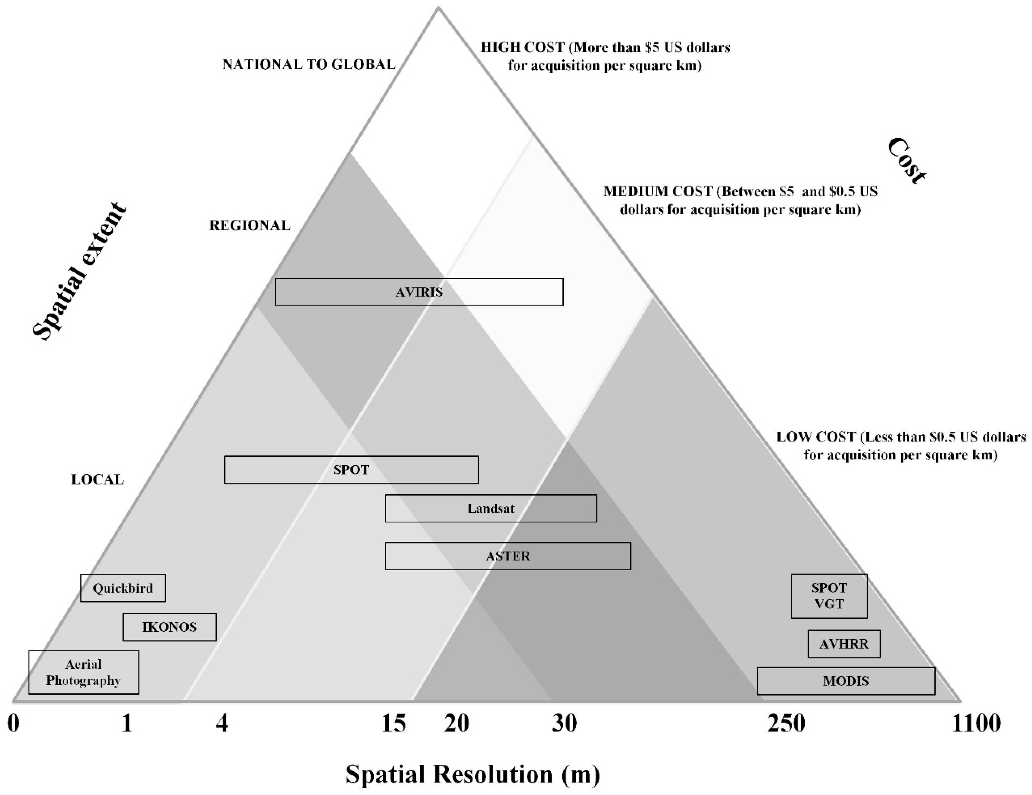
4.2. Remote Sensing as a Tool to Identify Potential GDEs

Field campaigns to determine the location of GDEs are able to provide high quality maps with high spatial resolution. However, field-based inventories of GDEs are not convenient when maps covering large areas (state-wide, regional, national, or global), remote locations, and long-term changes are required. Field surveys to determine the location of GDEs are labor intensive, expensive, and represent just one point in time. The key motivations for the use of remote sensing technology to identify the location of GDEs are:

• For the sustainable management of natural resources, the implementation of effective and cost-efficient techniques (such as remote sensing) to identify and monitor GDEs at levels broader than the field level is critical [87].
• The only practical approach to identify and monitor GDEs at a regional level or larger is to take advantage of remote sensing capabilities.

Several types of airborne and spaceborne instruments can be used to map GDEs. Aerial photographs provide a consistent long-term historical record of surface conditions and variations. Several landscape patterns that can be linked with groundwater are clearly identified on aerial photographs. These include [88]: greater amounts of green vegetation cover than expected; darker soils due to high soil moisture or carbon levels caused by anoxic soil conditions; and changes in plant community type that are related to water availability. Light detection and ranging (LIDAR) is a remote sensing technology that can be used for the production of highly accurate digital elevation models which are essential to obtain topographic metrics (e.g., slope, aspect and topographic wetness index). These topographic metrics have successfully been used to locate GDEs [89,90]. Radar imagery has also been used to derive ground-surface information on GDEs [91,92,93,94]. Synthetic Aperture Radar (SAR) is particularly successful in providing information about moisture inundation, seasonal fluctuations of the water table, vegetation patterns, and impact of natural and anthropogenic disturbance [95]. Radar measurements allow investigation of the water balance of GDEs and hydrologic boundary conditions, assuming that the water body is the surface expression of groundwater [88]. Remote sensing techniques to identify GDEs also include the use of the thermal infrared band to map locations associated with high levels of evapotranspiration and/or saturation [87]. High resolution airborne multispectral and thermal infrared imagery was acquired over the Mojave River, California to estimate evapotranspiration and water use by riparian vegetation [96], thermal infrared remote sensing of vegetation temperature was integrated with a surface energy balance model to efficiently calculate spatially distributed evapotranspiration [97], and LANDSAT Thematic Mapper (TM) thermal infrared band was used for the classification of successional stages of forest growth [98]. Low altitude aerial infrared surveys making use of thermal infrared cameras have also been found to be extremely useful to investigate the interactions between groundwater and surface water [99].

The satellite sensors that are most suitable for extraction of information valuable for mapping and monitoring GDEs are presented in Figure 1. Sensor suitability for a specific application depends on the resolving power of the sensor, namely the spatial, temporal, radiometric, and spectral resolution. For this reason, one of the crucial activities when using remote sensing for GDE mapping is the careful selection of the suitable dataset that can provide information with the required quality, at the required spatial and temporal resolution. However, the choice of using a given sensor is typically limited by the cost of the satellite imagery [9]. Figure 1 can be used for the selection of remote sensing imagery for GDE detection (from the satellite instrumens that are suitable in terms of spectral and radiometric resolution) considering the cost of acquisition of the image per km² [55], the spatial resolution required, and the spatial extent of the studies. Additionally, a review of previous studies in which products from these sensors have been used for identifying the location and extent of GDEs is presented in

Table 1. Main features of the most suitable sensors for delineation of GDEs and studies that have focused on the use of these technologies.

Satellite Sensor	Characteristics	Mapping Scale	Applications	Studies That Identify GDEs Using These Sensors
ASTER	Low to medium spatial resolution. VNIR bands (15 m), SWIR bands (30 m), TIR bands (90 m)	1:24,000–1:100,000	Ecosystem dynamics, geology and soils, land cover change, digital elevation models (DEMs), and vegetation mapping at species or community level	[100,101]
AVHRR	Low spatial resolution (1 km)	1:100,000–1:1,000,000	Global terrestrial ecosystem monitoring; mapping of land cover types	[102]
AVIRIS	Airborne optical sensor that delivers images in 224 contiguous spectral channels at varying spatial resolution (4 m to 30 m)	1:24,000–1:100,000	Vegetation leaf water, biomass assessment, vegetation mapping at species or community level	[103]
Hyperion	Low spatial resolution (30 m).	1:24,000–1:100,000	Biomass, LAI, vegetation mapping at species or community level	[104]
IKONOS	High to medium spatial resolution. 1 m (panchromatic imagery) and 4 m (multispectral bands including VIS and NIR).	1:4,000–1:24,000	Vegetation mapping at species or community level, urban and rural mapping of natural resources, and change detection.	[105]
LANDSAT ETM+	Medium to coarse spatial resolution with multispectral data. 15 m (panchromatic band), 30 m (multispectral bands), 60 m (TIR band).	1:24,000–1:100,000	Photosynthetic activity assessment, vegetation mapping at community level, land cover and change detection.	[57,106]
LANDSAT TM	Medium to coarse spatial resolution with multispectral data. 30 m (multispectral bands), 120 m (TIR band).	1:24,000–1:100,000	Photosynthetic activity assessment, vegetation mapping at community level, land cover and change detection.	[23,81,87,107]
MODIS	Low spatial resolution (250—1000 m) and multispectral data	1:100,000–1:1,000,000	Photosynthetic Activity trends, land cover/vegetation mapping and monitoring, evapotranspiration estimation,	[57,81,101,108]
Quickbird	High spatial resolution (0.65—2.4 m). Panchromatic and multispectral bands	1:4,000–1:24,000	Land-cover and land-use monitoring, vegetation mapping at species or community level	[101]
SPOT	Medium spatial resolution (1.5 m to 20 m)	1:24,000–1:100,000	Land-cover and land-use monitoring, vegetation mapping at species or community level	[109]

[23,57,81,87,100,101,102,103,104,105,106,107,108,109], with details regarding the main characteristics (such as spatial resolution and mapping scales) of each sensor and applications that have benefited from and could potentially take advantage of the sensors’ capabilities to map GDEs. The approximate mapping scale for which each sensor can be used (Column 3) is based on the spatial resolution of the data.

The process of mapping GDEs utilizing remote sensing technologies consists of the interpretation of remotely sensed imagery using techniques to extract information and/or derive indicators that can exploit potential distinction between GDEs and surrounding land cover. Interpretation elements that are commonly used for vegetation and ecological mapping are image color, tone, texture, and pattern [110]. Overall, the mapping process involves image preprocessing and image classification. The preprocessing of satellite images includes initial steps that remove noise and increase the interpretability of the data such as atmospheric corrections. This is of particular importance when several scenes are being used for a given study for multi-temporal analysis, change detection, or for assessment of large areas that encompass more than one scene. On the other hand, image classification is concerned with the extraction of classes or clusters from the remotely sensed information using traditional classification algorithms or improved classifiers. Traditional methods include K-means and ISODATA (unsupervised classification methods), as well as maximum likelihood classification (supervised classification technique). Elmore et al. [111] developed an approach to characterize the response of groundwater dependent terrestrial vegetation and non-GDEs to human disturbance (particularly groundwater extraction) in Owens Valley, CA based on the interpretation of LANDSAT imagery. The image preprocessing consisted of co-registration of the dataset, calibration to a common spectral response, geo-referencing, and analysis using spectral mixture analysis. For the image classification, an ISODATA-clustering algorithm was implemented. Improved methods are obtained from the traditional methods, but they usually expand on particular techniques that can lead to better results. These improved methods are commonly used when GDEs or vegetation types display similar spectral characteristics in the image, making it difficult to classify them accurately [110].

Another remote sensing technique that has been widely used to map potential GDEs is the derivation of remote sensing indicators such as the Normalized Difference Vegetation Index (NDVI), which is a numerical indicator that makes use of the red and near-infrared bands of the electromagnetic spectrum to determine the vegetation status and photosynthetic activity in a given area. This indicator has been used in several studies to identify terrestrial ecosystems and wetlands that depend on groundwater based on the principle that ecosystems that are able to maintain consistent greenness during a prolonged dry period, are defined as potentially groundwater dependent [57,81,107,108]. Other indicators of vegetation density, health, and condition that have been used are the Enhanced Vegetation Index (EVI) and remotely-sensed Leaf Area Index (LAI), as well as indicators of moisture dynamics like the Normalized Difference Wetness Index (NDWI), and tasseled cap (TC) wetness and greenness. A study focused on the use of a satellite-based approach based on EVI as a proxy for evapotranspiration anomalies to estimate water consumption by ecosystems in arid and semi-arid regions of central Argentina [112]. Barron et al. [107] successfully applied a methodology in Western Australia, which consisted of the interpretation of the land surface response to the drying process, based on the satellite-obtained indices NDVI and NDWI, to infer the location of GDEs.

Of particular importance to the identification and study of GDEs is the Gravity Recovery and Climate Experiment (GRACE) satellite launched on March 2002 to map variations in the Earth's gravity field. After removal of atmospheric and oceanic effects, temporal changes of Earth’s gravitational potential are mostly caused by changes in terrestrial water storage [113]. For this reason, the measurements from GRACE make a huge contribution in studies focused on understanding variations of groundwater storage on land masses, although this contribution is limited by GRACE’s coarse effective spatial resolution of several hundred kilometers. Sun et al. [113] developed a non-parametric approach to statistically downscale changes in terrestrial water storage obtained from GRACE to predict groundwater level changes. Results show that the relative importance of GRACE to water level change prediction ranges from 8% to 20% proving that GRACE measurements can be extremely valuable for tracking groundwater level changes to manage aquifers in a sustainable manner. Other studies relevant in the process of understanding the role of hydrologic fluxes and storages on terrestrial water distribution have focused on studying continental water storage changes using GRACE [114], evaluation of GRACE data for understanding elements of hydrologic systems in drainage basins [115,116,117], and monitoring of groundwater storage variations in aquifers where groundwater is being depleted [118,119,120,121,122,123,124]. Future work still remains to determine if GDEs are less vulnerable to short-term drought than rain-dependent ecosystems and if, depending to some extent on groundwater dynamics, GDEs are vulnerable to long-term drought or to chronic water diversion [119,125]. Shorth-term and long-term droughts can both be assessed, albeit at a coarse spatial scale, by reduction in GRACE measured water storage [114].

Limitations of Using Remote Sensing to Detect GDEs

Several studies have noted that a major limitation of using remote sensing technologies to map GDEs is that the size of some ecosystems (e.g., seeps, spring groups, and individual springs) is usually smaller than the size of an individual pixel in the available remotely sensed imagery. Consequently, the remote sensing dataset does not clearly show the feature and instead the pixel value represents a mixture of several features within the pixel [87,101]. Another obstacle in the accurate detection of GDEs using remote sensing datasets is that some of these ecosystems present spectral characteristics that are not easily distinguishable from the adjacent land cover, making it difficult to delineate them.

4.3. Integration of Remotely Sensed Data with Ground-Based Observations for Identification of GDEs

Sustainable management of ecosystems is supported by research that is focused on the characterization of ecosystem condition and change, understanding the impact of distinct management approaches, and evaluation of the natural and human influence on ecosystem functions. These research activities can greatly benefit from having a field-based scientific inventory of resources (e.g., soil and water) that can be used to understand the differences between ecosystems that are supported by groundwater and those that are not, but they can also be complemented by remote sensed technology because it provides cost-effective ways to monitor and study large and remote areas, extending data archives from present to several decades back [110]. The integration between remotely sensed data and ground-based observations is commonly accomplished using GIS technology. A GIS is a computer-based tool that combines database operations, such as query and statistical analysis, with maps. GIS provides tools to query, manage, manipulate, overlay, analyze, visualize and store all forms of geographically referenced information.

In many cases, the process of integration between ground-based observations and remotely sensed data for the purpose of identifying and characterizing GDEs starts by deriving information from ground-based data using GIS technologies. This is accomplished by analyzing and manipulating ground-based observations using geostatistical methods. Geostatistics is a group of numerical techniques for the characterization of spatial attributes using probabilistic models and pattern recognition techniques. Geostatistics are used to generate surfaces from ground-based observations using interpolation methods such as global and local polynomials, kriging, and radial basis functions. These interpolation methods can also provide new surfaces from data that was acquired using remote sensing technologies, such as calculating slope and aspect from a topographic map that was produced by photogrammetric techniques using aerial images [126]. Studies that benefit from this integration have developed a number of indexes that compile major variables that influence groundwater dependence [127,128].

Several authors have documented the ecosystem response to landforms and how the composition and structure of vegetation is determined by geomorphic events [85,129]. Landforms (usually characterized by topography and geology) deeply influence spatial variations in ecological variables such as water availability and exposure to radiant solar energy. Landforms are linked with climate through varying heights and degree of ground-surface inclination, controlling the intensity of key factors (such as hydrology) important to plants and to the soil-forming processes [130]. Using geostatistics, elevations measured by different techniques (e.g., field surveying, photogrammetry, and cartographic digitization) [131] are interpolated with the purpose of creating a DEM from interpolated elevations. Groundwater dependent wetlands and springs usually occur in topographies associated with depressions and flat areas that lack drainage outlets and/or are subject to flooding, and they are also common in locations where groundwater discharges, which makes the area wet for extended periods of time. In the discharge areas, due to a constant supply of groundwater, a perennial moisture excess exists at and near the land surface as compared to the amount of ground moisture that would result from a balance of precipitation and evapotranspiration [132]. Therefore, field collected observations of soil moisture and location of inundation areas can be combined with topographic derivatives derived from DEMs to help discriminate GDEs from non-GDEs.

Since not all wetlands are supported by groundwater, one way to determine the wetlands’ water source is to investigate the wetland soils because these can provide a suggestion of a continuous influx of groundwater to the ecosystem. They may be found in soil survey maps as hydric soils because they are usually formed when saturated conditions persist for a prolonged period [74]. GIS technologies can serve the purpose of integrating ground-based data and satellite imagery for the purpose of providing broad-based inventory of soils with information about their physical and chemical properties that can be used to map ecosystems. One example of this kind of products is the October 1994 State Soil Geographic (STATSGO) database provided by the USGS. This map is the result of assembling detailed field-based inventories of soils, data on geology, topography, vegetation, and climate, and information extracted from Land Remote Sensing Satellite (Landsat) images [133].

5. Review of Case Studies for GDE identification at Different Spatial Extents

5.1. Detection of GDEs at the Local Level

In Australia, [108] focused on the Hat Head National Park located in New South Wales. Their study consisted of the development of an approach based on the combination of a GIS vegetation layer with calculated water table surface and MODIS Enhanced Vegetation Index (EVI) time series data. The estimated water table depth was obtained by subtracting surface elevation (acquired as a Digital Elevation Model (DEM)) from modelled head values. This assessment involved the distinction between facultative and obligate GDEs.

In the United States, [87] devised a method based on the combination of reference data and geospatial data layers (data organized in themes using GIS software). The reference data was derived from the interpretation of aerial imagery and using information collected in the field. On the other hand, the geospatial layers were obtained from remote sensing data and digital elevation models. The purpose was to locate potential GDEs in two different areas. The first was the Springs Mountains National Recreation Area located in Nevada in which the predominant GDEs are springs. The second area was the Grand Mesa landform, located in Colorado, in which a large number of fens have been identified. A system based on statistical methods such as the best predictor variables and hierarchical clustering was created to evaluate the strength of the association between the geospatial data layers and the reference data. Decision trees were created and a classification was performed. Results showed that the data-dependent method was limited in its ability to capture the features of GDEs where ground-based data was restricted in amount. For this reason, approaches that are based on the combination of field measurements and remote sensing data can be more convenient in the detection of GDEs. A more recent study developed a random forest methodology where many regression trees were constructed using multiple geospatial and remote sensing data layers to identify areas with shallow water table, which have the most potential to harbor GDEs, in Nevada [90].

Another study was carried out in the Beartooth Mountains of Wyoming [100]. This was focused on peatlands, which are defined as GDEs when they are supported by groundwater. These types of peatlands are typically found in lower topographic areas where minerals are present in the groundwater and are called minerogenous or minerotrophic peatlands. Another type of peatlands, ombrotrophic fen, is not considered as GDE [86]. In the Beartooth Mountains, the peatland systems present are minerotrophic fens, which are classified as groundwater reliant. This study was successful in documenting peatlands by using a combination of aerial photo-interpretation, evaluation of soil maps for histosol units, and field verification. The resulting map showed more than 150 peatland sites located over 150 square miles. Additionally, a pilot remote sensing assessment that included LANDSAT (30 m), ASTER (15 m), and CIR aerial photos (1 m) was conducted. This study provided a framework for tailoring remote sensing tools to the variety of peatland features and presented the benefits from using field-based inventories to refine results derived from remote sensing data.

5.2. Assessments of Groundwater Dependency in Different States

Several studies have focused on the development of methodologies to create GDE maps for different states in the USA. A method was devised to map the distribution of GDEs in California [127]. Groundwater dependence was shown down to the finest USGS hydrologic unit scale (HUC12), which represents a mean size of 9570 hectares (cell area of approximately 100 km²). Geospatial datasets to identify locations of GDEs were compiled and analyzed to develop an index of groundwater dependency. The index is created by ranking three ecosystem types: springs and seeps, wetlands, and streams.

Another assessment of the distribution of GDEs and possible threats to the groundwater supply was conducted by the Nature Conservancy in Oregon [128,134]. A GIS-based model was created in which results are summarized at the 6th level Hydrologic Unit Code (HUC6) which represents a mean size of 8055 ha. The study focused on the identification of species and plant communities of conservation concern that rely on groundwater and four different types of GDEs: wetlands, river base flow systems, springs, and lakes. The approach was based on two steps. The first step consisted of identifying the location of these ecosystems using a variety of information such as ecoregional assessments, gage data, aerial photos, and remote sensing products. Then, a set of criteria developed for each ecosystem to evaluate the importance of groundwater was implemented. After mapping HUC6s, which contained GDEs, the distribution of GDEs was summed up by defining a GDE cluster according to the number of GDEs identified in a particular HUC6 sub-area. This methodology was also applied in Washington State to increase the knowledge about the location of GDEs in the United States Pacific Northwest region [134].

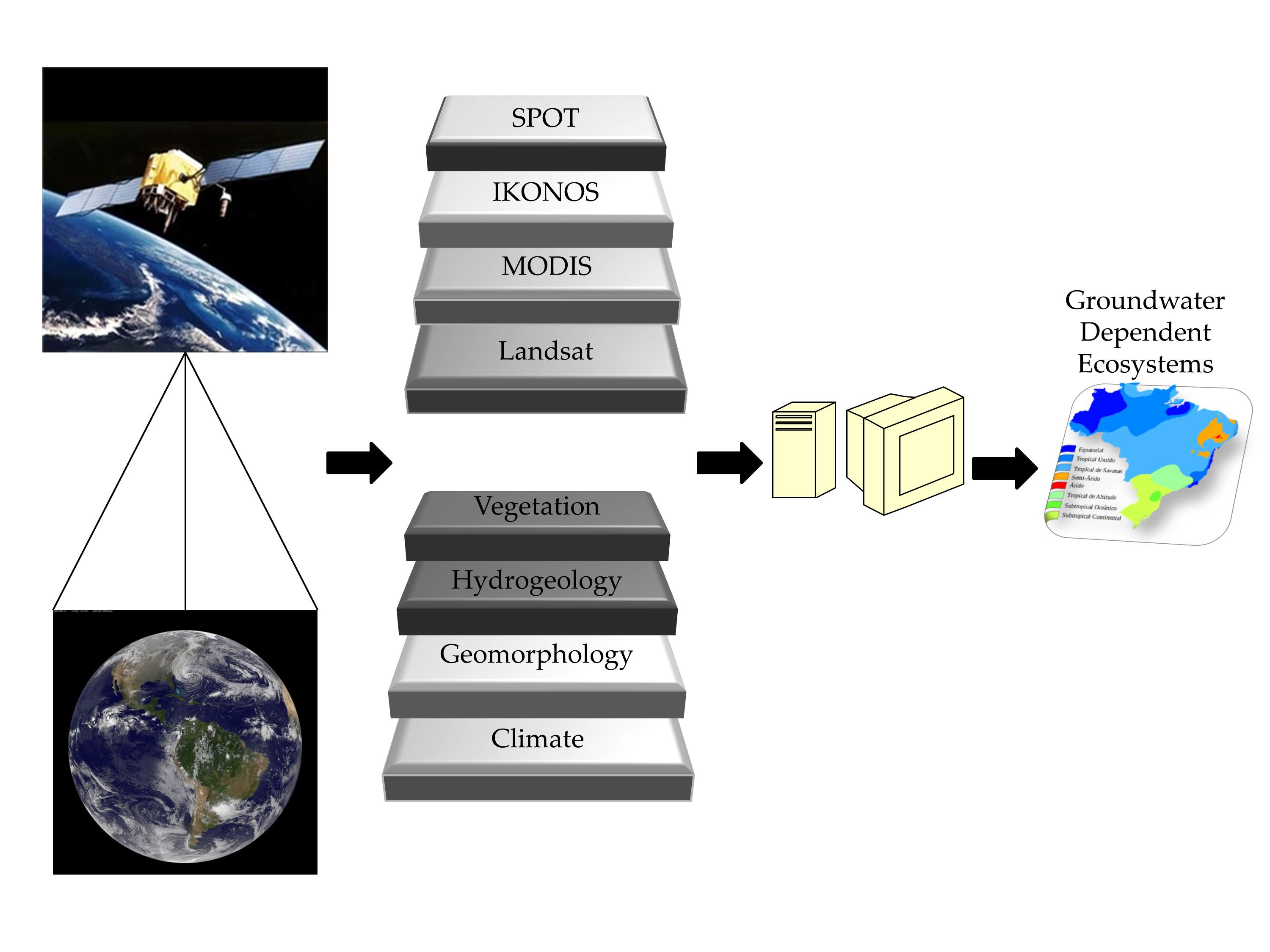
5.3. Identification of GDEs at the National and Regional Level

Significant efforts to map the location and extent of GDEs at a national level have been undertaken in only two countries. In Australia, an operational GDE atlas was produced by combining previously identified GDEs, available literature, geospatial layers and remote sensing data [135]. The approach was based in analysis rules developed for eight different analysis regions in which conditions such as climate, ecology, and hydrogeology were considered similar. Within each region, analysis rules were applied using GIS technologies and then rated to infer locations where interaction between groundwater and the ecosystem was probable. This map represents the most exhaustive inventory of GDEs that has been accomplished for a country.

In South Africa, [9] produced a national map of GDEs depicting the probability of occurrence of terrestrial groundwater dependent ecosystems according to two indicators. First, groundwater levels, since plants will use water in proportion to its availability. Water levels are obtained as annual means based on a national database. The second indicator to evaluate dependency is duration of the moisture growing season, defined as precipitation-derived water that can be used by terrestrial vegetation in the form of soil moisture. This was calculated using values of precipitation and evaporation obtained by analysis of long-term meteorological data. The national map was created by assigning ratings to the indicator values. This type of assessment was conducted as a preliminary and coarse identification of ecosystems, meant to be utilized at a watershed management level.

The major assessment that has been undertaken for the United States is a map depicting the phreatophytic land cover of the northern and central Great Basin Ecoregion including the states of California, Nevada, Utah, Idaho, Oregon, and Wyoming was prepared by the USGS [13]. The approach to delineate coverage of phreatophytes was based on geospatial analysis of available land cover datasets such as Shrub Map, California GAP, and Wyoming GAP. The first step was to identify and combine vegetation classes that were thought to utilize groundwater. Then, their distribution was evaluated and the resulting map was overlapped with slope and relief information which are considered to be able to capture, at a regional scale, plant communities that are better able to develop dependence on groundwater because of their location in areas of shallow groundwater.

On the western coast of South Africa, particularly the Northern Sandveld, [136] integrated remote sensing and botanical field mapping using GIS technologies, in an area with high proportion of groundwater-fed wetlands to detect probable GDEs. In the same region, [23] utilized aerial photography in conjunction with analysis of LANDSAT-derived indicators to map riverine and wetland GDEs, refined with the use of GIS terrain modeling. This study considered in the GIS terrain model, critical factors that influence groundwater dependence such as water table depth and geological fractures.

6. Conclusions

Groundwater extraction is one of the major causes of ecosystem change and has been notably substantial in the past five decades. It is clear that the protection of ecosystems that are supported by groundwater is imperative given the growing risk of depletion of groundwater resources in most parts of the world. In order to be able to manage groundwater and ecosystems, it is necessary to consider the water requirements of GDEs together with the freshwater requirements of a growing population. The first step in the process of adequately allocating water resources is to identify the location and extent of GDEs, as well as the nature and degree of the dependence.

Collection of field survey data is useful for inventorying and mapping of ecosystems at a fine spatial scale. Field data is important because of the high confidence that can be placed on variables that are adequately collected. For this reason, they are also crucial for the validation of data sets acquired using remote sensing technologies. However, this type of data lacks the temporal extent, spatial coverage, and cost-effectiveness that are found in remote sensing data. On the other hand, remote sensing and GIS technologies have revolutionized the way in which environmental data are collected, stored, analyzed, and visualized. The advantages of remote sensing for GDEs mapping and monitoring include the possibility of collecting data for large and remote areas, as well as regular temporal coverage. Satellite imagery analyzed using GIS can also be extremely valuable because it provides spatially continuous data, validated and complemented by sample field data points. GIS technology can assist in the delineation of GDEs in several ways, which include spatial modeling capabilities to utilize and combine key factors that affect ecosystem distribution. The successful use of remote sensing technologies to map GDEs relies on the size of features being larger than the pixel size and on understanding the spectral signatures that distinguish GDEs from non-GDEs.

Successful attempts to characterize and delineate GDEs at local and statewide level have been reported, but much work still remains in the development of technologies able to identify and characterize GDEs at broader extents. Integration of field survey data collection and remote sensing using GIS have the greatest potential because detailed observations can be used to understand the differences between ecosystems that are supported by groundwater and those that are not. The poor spatial and temporal coverage of field observation could be complemented by satellite imagery that provides cost-effective ways to monitor large and remote areas. In places where there is confusion between spectral signatures, or the quality of the available imagery is not adequate, GIS technologies can provide assistance in the process of updating ecological data by combining multiple spatial layers and scattered field data to delineate the areas most likely to contain GDEs. This integration will result in more consistent and objective maps of the ecosystems that depend on groundwater. Field methods can prove useful to investigate spatio-temporal variability of groundwater dependence of ecosystems at a local level. However, satellite-derived data is a more suitable alternative for the determination and evaluation of hydrogeological processes that cover larger areas. This integration of field-collected data and remote sensing is still a challenge in the delineation of GDEs because of poor development of automated techniques for this integration, differing formats and scattered storage locations of field observational data, and scarcity of geospatial data with high spatial resolution. Data mining techniques useful for the non-trivial extraction of implicit information from predictor variables should be investigated in the future for the purpose of identifying GDEs. Data mining algorithms might be able to find hidden patterns between GDEs and different predictor variables that may otherwise be missed because they are not expected, although guidance by ecohydrological experts is still needed to ensure that the obtained models are plausible and generalizable [137]. Ground-based measurements of water table depth as well as field-based inventories of wetlands, springs, and phreatophytes can potentially be used as training data in models developed to predict the presence of GDEs using remote sensing, climate, and topography variables as predictors.

One challenge for the identification of GDEs is the uncertainty as to whether ecosystems are actually groundwater dependent or just using groundwater even though it is not required for their survival (facultative versus obligate GDEs). This means that a better understanding of the coupling between climate, groundwater, vegetation, and soil water is necessary to accurately characterize the feedback between ecosystem and hydrological processes. As well, uncertainties associated with field-based inventories and remote sensing data products must be known. This is crucial in the process of understanding their influence on the results.

References

1. Millenium Ecosystem Assessment. Ecosystems and Human Well-being: Synthesis; Island Press: Washington, DC, USA, 2005. [Google Scholar]
2. Lawford, R.; Strauch, A.; Toll, D.; Fekete, B.; Cripe, D. Earth observations for global water security. Curr. Opin. Environ. Sustain. 2013, 5, 633–643. [Google Scholar] [CrossRef]
3. Margat, J.; van der Gun, J. Groundwater Around the World: A Geographic Synopsis; CRC Press/Balkema: London, UK, 2013. [Google Scholar]
4. Villholth, K.G.; Giordano, M. Groundwater use in a global perspective: Can it be managed? In The Agricultural Groundwater Revolution: Opportunities and Threats to Development; CAB International: Oxfordshire, UK, 2007; pp. 393–402. [Google Scholar]
5. Groundwater Facts. Available online: http://www.ngwa.org (accessed on 5 October 2014).
6. Moran, T.; Choy, J.; Sanchez, C. The Hidden Costs of Groundwater Overdraft. Available online: http://waterinthewest.stanford.edu/groundwater/overdraft/ (accessed on 10 September 2014).
7. Schmoll, O.; Howard, G.; Chilton, J.; Chorus, I. Protecting Groundwater for Health: Managing the Quality of Drinking-Water Sources; IWA Publishing: London, UK, 2006; pp. 1–175. [Google Scholar]
8. Foster, S.; Koundouri, P.; Tuinhof, A.; Kemper, K.; Nanni, M.; Garduño, H. Groundwater Dependent Ecosystems: The Challenge of Balanced Assessment and Adequate Conservation; The World Bank: Washington, DC, USA, 2006. [Google Scholar]
9. Colvin, C.; Le Maitre, D.; Hughes, S. Assessing Terrestrial Groundwater Dependent Ecosystems in South Africa; Water Research Commission: Pretoria, South Africa, 2003. [Google Scholar]
10. Merz, S.K.; Evans, R.; Clifton, C.A. Environmental Water Requirements to Maintain Groundwater Dependent Ecosystems; Commonwealth of Australia: Canberra, Australia, 2001. [Google Scholar]
11. Glasser, S.; Gauthier-Warinner, J.; Keely, J.; Gurrieri, J.; Tucci, P.; Summers, P.; Wireman, M.; McCormack, K. Technical Guide to Managing Ground Water Resources; United States Department of Agiculture: Washington, DC, USA, 2007.
12. Eamus, D. Identifying Groundwater Dependent Ecosystems: A Guide for Land and Water Managers; Land & Water Australia: Braddon, Australia, 2009.
13. Mathie, A.M.; Welborn, T.L.; Susong, D.D.; Tumbusch, M.L. Phreatophytic Land-Cover Map of the Northern and Central Great Basin Ecoregion: California, Idaho, Nevada, Utah, Oregon, and Wyoming; US Department of the Interior, US Geological Survey: Reston, VA, USA, 2011.
14. Stone, E.L.; Kalisz, P.J. On the maximum extent of tree roots. For. Ecol. Manage. 1991, 46, 59–102. [Google Scholar] [CrossRef]
15. Jyväsjärvi, J.; Marttila, H.; Rossi, P.M.; Ala-Aho, P.; Olofsson, B.; Nisell, J.; Backman, B.; Ilmonen, J.; Virtanen, R.; Paasivirta, L.; et al. Climate-induced warming imposes a threat to north European spring ecosystems. Glob. Chang. Biol. 2015, 21, 4561–4569. [Google Scholar] [CrossRef] [PubMed]
16. Dams, J.; Salvadore, E.; Van Daele, T.; Ntegeka, V.; Willems, P.; Batelaan, O. Spatio-temporal impact of climate change on the groundwater system. Hydrol. Earth Syst. Sci. 2012, 16, 1517–1531. [Google Scholar] [CrossRef] [Green Version]
17. Harding, C.; Deane, D.; Green, G.; Kretschmer, P. Impacts of Climate Change on Water Resources in South Australia Phase 4, Volume 2 Predicting the Impacts of Climate Change to Groundwater Dependent Ecosystems; Department of Environment, Water and Natural Resources: Adelaide, Australian, 2015.
18. Kumar, C.P. Climate Change and Its Impact on Groundwater Resources. Int. J. Eng. Sci. 2012, 1, 2278–4721. [Google Scholar]
19. Green, T.R.; Taniguchi, M.; Kooi, H.; Gurdak, J.J.; Allen, D.M.; Hiscock, K.M.; Treidel, H.; Aureli, A. Beneath the surface of global change: Impacts of climate change on groundwater. J. Hydrol. 2011, 405, 532–560. [Google Scholar] [CrossRef]
20. Kløve, B.; Ala-aho, P.; Bertrand, G.; Gurdak, J.J.; Kupfersberger, H.; Kværner, J.; Muotka, T.; Mykrä, H.; Preda, E.; Rossi, P.; et al. Climate change impacts on groundwater and dependent ecosystems. J. Hydrol. 2013, 518, 250–266. [Google Scholar] [CrossRef]
21. Taylor, R.G.; Scanlon, B.; Doll, P.; Rodell, M.; van Beek, R.; Wada, Y.; Longuevergne, L.; Leblanc, M.; Famiglietti, J.S.; Edmunds, M.; et al. Ground water and climate change. Nat. Clim. Chang. 2012, 3, 322–329. [Google Scholar] [CrossRef] [Green Version]
22. MacKay, H. Protection and management of groundwater-dependent ecosystems: Emerging challenges and potential approaches for policy and management. Aust. J. Bot. 2006, 54, 231–237. [Google Scholar] [CrossRef]
23. Münch, Z.; Conrad, J. Remote sensing and GIS based determination of groundwater dependent ecosystems in the Western Cape, South Africa. Hydrogeol. J. 2006, 15, 19–28. [Google Scholar] [CrossRef]
24. De Smith, M.J.; Goodchild, M.F.; Longley, P.A. Geospatial Analysis: A Comprehensive Guide to Principles, Techniques and Software Tools, 5th ed.; The Winchelsea Press: Winchelsea, UK, 2015. [Google Scholar]
25. Batelaan, O.; Witte, J.P.M. Ecohydrology and Groundwater Dependent Terrestrial Ecosystems. In Proceedings of the 28th Annual Conference of the International Association of Hydrogeologists (Irish Group), Tullamore, Ireland, 22–23 April 2008; pp. 1–8.
26. Rodriguez-Iturbe, I. Ecohydrology : A hydrologic perspective of climate-soil-vegetation dynamics. Water Resour. Res. 2000, 36, 3–9. [Google Scholar] [CrossRef]
27. Froend, R.; Loomes, R.; Horwitz, P.; Bertuch, M.; Storey, A.; Bamford, M. Study of Ecological Water Requirements on the Gnangara and Jandakot Mounds under Section 46 of the Environmental Protection Act. Task 2: Determination of Ecological Water Requirements; Centre for Ecosystem Management: Perth, Australia, 2004. [Google Scholar]
28. Kløve, B.; Ala-aho, P.; Bertrand, G.; Boukalova, Z.; Ertürk, A.; Goldscheider, N.; Ilmonen, J.; Karakaya, N.; Kupfersberger, H.; Kvoerner, J.; et al. Groundwater dependent ecosystems. Part I: Hydroecological status and trends. Environ. Sci. Policy 2011, 14, 770–781. [Google Scholar] [CrossRef]
29. Kløve, B.; Allan, A.; Bertrand, G.; Druzynska, E.; Ertulk, A.; Goldscheider, N.; Henry, S.; Karakay, N.; Karjalainen, T.; Koundouri, P.; et al. Groundwater dependent ecosystems. Part II. Ecosystem services and management in Europe under risk of climate change and land use intensification. Environ. Sci. Policy 2011, 14, 782–793. [Google Scholar] [CrossRef]
30. Laio, F.; Tamea, S.; Ridolfi, L.; D’Odorico, P.; Rodriguez-Iturbe, I. Ecohydrology of groundwater-dependent ecosystems: 1. Stochastic water table dynamics. Water Resour. Res. 2009, 45. [Google Scholar] [CrossRef]
31. Guswa, A.J.; Celia, M.; Rodriguez-Iturbe, I. Models of soil moisture dynamics in ecohydrology: A comparative study. Water Resour. Res. 2002, 38. [Google Scholar] [CrossRef]
32. Guswa, A.J. Soil-moisture limits on plant uptake: An upscaled relationship for water-limited ecosystems. Adv. Water Resour. 2005, 28, 543–552. [Google Scholar] [CrossRef]
33. Laio, F. A vertically extended stochastic model of soil moisture in the root zone. Water Resour. Res. 2006, 42, 1–10. [Google Scholar] [CrossRef]
34. Laio, F.; Porporato, A.; Fernandez-Illescas, C.; Rodriguez-Iturbe, I. Plants in water-controlled ecosystems: Active role in hydrologic processes and response to water stress. Adv. Water Resour. 2001, 24, 745–762. [Google Scholar] [CrossRef]
35. Porporato, A.; D’Odorico, P.; Laio, F.; Ridolfi, L.; Rodriguez-Iturbe, I. Ecohydrology of water-controlled ecosystems. Adv. Water Resour. 2002, 25, 1335–1348. [Google Scholar] [CrossRef]
36. Rodríguez-Iturbe, I.; Porporato, A. Ecohydrology of Water-Controlled Ecosystems. Soil Moisture and Plant Dynamics; Cambridge University Press: Cambridge, UK, 2004. [Google Scholar]
37. Rodriguez-Iturbe, I.; Porporato, A.; Ridolfi, L.; Isham, V.; Coxi, D.R. Probabilistic modelling of water balance at a point: The role of climate, soil and vegetation. Proc. R. Soc. Lond. A: Math. Phys. Eng. Sci. 1999, 455, 3789–3805. [Google Scholar] [CrossRef]
38. Tamea, S.; Laio, F.; Ridolfi, L.; D’Odorico, P.; Rodriguez-Iturbe, I. Ecohydrology of groundwater-dependent ecosystems: 2. Stochastic soil moisture dynamics. Water Resour. Res. 2009, 45. [Google Scholar] [CrossRef]
39. Salvucci, G.D.; Entekhabi, D. Equivalent steady soil moisture profile and the time compression approximation in water balance modeling. Water Resour. Res. 1994, 30, 2737–2749. [Google Scholar] [CrossRef]
40. Ridolfi, L.; D’Odorico, P.; Laio, F.; Tamea, S.; Rodriguez-Iturbe, I. Coupled stochastic dynamics of water table and soil moisture in bare soil conditions. Water Resour. Res. 2008, 44, 1–11. [Google Scholar] [CrossRef]
41. Eagleson, P.S. Climate, soil, and vegetation: 3. A simplified model of soil moisture movement in the liquid phase. Water Resour. Res. 1978, 14, 722–730. [Google Scholar] [CrossRef]
42. D’odorico, P.; Laio, F.; Porporato, A.; Ridolfi, L.; Rinaldo, A.; Rodriguez, I. Ecohydrology of terrestrial ecosystems. Bioscience 2010, 60, 898–907. [Google Scholar] [CrossRef]
43. Rodriguez-Iturbe, I.; D’Odorico, P.; Laio, F.; Ridolfi, L.; Tamea, S. Challenges in humid land ecohydrology: Interactions of water table and unsaturated zone with climate, soil, and vegetation. Water Resour. Res. 2007, 43, 1–5. [Google Scholar] [CrossRef]
44. Ahring, T.S.; Steward, D.R. Groundwater surface water interactions and the role of phreatophytes in identifying recharge zones. Hydrol. Earth Syst. Sci. 2012, 16, 4133–4142. [Google Scholar] [CrossRef] [Green Version]
45. Ala-aho, P.; Rossi, P.M.; Isokangas, E.; Kløve, B. Fully integrated surface-subsurface flow modelling of groundwater-lake interaction in an esker aquifer: Model verification with stable isotopes and airborne thermal imaging. J. Hydrol. 2015, 522, 391–406. [Google Scholar] [CrossRef]
46. Brookfield, A.E.; Sudicky, E.A.; Park, Y.J.; Conant, B., Jr. Thermal transport modelling in a fully integrated surface/subsurface framework. Hydrol. Process. 2009, 23, 2150–2164. [Google Scholar] [CrossRef]
47. Trigg, M.A.; Cook, P.G.; Brunner, P. Groundwater fluxes in a shallow seasonal wetland pond: The effect of bathymetric uncertainty on predicted water and solute balances. J. Hydrol. 2014, 517, 901–912. [Google Scholar] [CrossRef]
48. Kollet, S.J.; Maxwell, R.M. Capturing the influence of groundwater dynamics on land surface processes using an integrated, distributed watershed model. Water Resour. Res. 2008, 44, 1–18. [Google Scholar] [CrossRef]
49. Krakauer, N.Y.; Puma, M.J.; Cook, B.I. Impacts of soil-aquifer heat and water fluxes on simulated global climate. Hydrol. Earth Syst. Sci. 2013, 17, 1963–1974. [Google Scholar] [CrossRef]
50. Fan, Y.; Li, H.; Miguez-Macho, G. Global patterns of groundwater table depth. Science 2013, 339, 940–943. [Google Scholar] [CrossRef] [PubMed]
51. Subin, Z.M.; Milly, P.C.D.; Sulman, B.N.; Malyshev, S.; Shevliakova, E. Resolving terrestrial ecosystem processes along a subgrid topographic gradient for an earth-system model. Hydrol. Earth Syst. Sci. Discuss. 2014, 11, 8443–8492. [Google Scholar] [CrossRef]
52. Fan, Y.; Krakauer, N.; Li, H. Groundwater flow across spatial scales: Importance for climate modeling. Environ. Res. Lett. 2014, 9, 034003. [Google Scholar]
53. Koirala, S.; Yeh, P.J.; Hirabayashi, Y.; Kanae, S.; Oki, T. Global-scale land surface hydrologic modeling with the representation of water table dynamics. 2014, 119, 75–89. [Google Scholar] [CrossRef]
54. Leng, G.; Huang, M.; Tang, Q.; Gao, H.; Leung, L.R. Modeling the effects of groundwater-fed irrigation on terrestrial hydrology over the conterminous United States. J. Hydrometeorol. 2014, 15, 957–972. [Google Scholar] [CrossRef]
55. Rogan, J.; Chen, D. Remote sensing technology for mapping and monitoring land-cover and land-use change. Prog. Plan. 2004, 61, 301–325. [Google Scholar] [CrossRef]
56. Grady, A.O.; Eamus, D.; Cook, P.; Lamontagne, S.; Kelly, G.; Hutley, L. Tree Water Use and Sources of Transpired Water in Riparian Vegetation along the Daly River, Northern Territory; Department of the Environment, Water, Heritage and the Arts: Sydney, Australia, 2003.
57. Gou, S.; Gonzales, S.; Miller, G.R. Mapping potential groundwater-dependent ecosystems for sustainable management. Groundwater 2014, 53, 99–110. [Google Scholar] [CrossRef] [PubMed]
58. Thorburn, P.J.; Walker, G.R.; Brunel, J.-P. Extraction of water from Eucalyptus trees for analysis of deuterium and oxygen-18: Laboratory and field techniques. Plant Cell Environ. 1993, 16, 269–277. [Google Scholar] [CrossRef]
59. Zencich, S.J.; Froend, R.H.; Turner, J.V.; Gailitis, V. Influence of groundwater depth on the seasonal sources of water accessed by Banksia tree species on a shallow, sandy coastal aquifer. Oecologia 2002, 131, 8–19. [Google Scholar] [CrossRef]
60. Smith, S.D.; Devitt, D.A.; Sala, A.; Cleverly, J.R.; Busch, D.E. Water relations of riparian plants from warm desert regions. Wetlands 1998, 18, 687–696. [Google Scholar] [CrossRef]
61. Jobbágy, E.G.; Nosetto, M.D.; Villagra, P.E.; Jackson, R.B. Water subsidies from mountains to deserts: Their role in sustaining groundwater-fed oases in a sandy landscape. Ecol. Appl. 2011, 21, 678–694. [Google Scholar] [CrossRef] [PubMed]
62. Rossi, P.M.; Marttila, H.; Jyväsjärvi, J.; Ala-aho, P.; Isokangas, E.; Muotka, T.; Kløve, B. Environmental conditions of boreal springs explained by capture zone characteristics. J. Hydrol. 2015, 531, 992–1002. [Google Scholar] [CrossRef]
63. Busch, D.E.; Ingraham, N.L.; Smith, S.D. Water uptake in woody riparian phreatophytes of the Southwestern United States: A stable isotope study. Ecol. Appl. 1992, 2, 450–459. [Google Scholar] [CrossRef]
64. McCole, A.A.; Stern, L.A. Seasonal water use patterns of Juniperus ashei on the Edwards Plateau, Texas, based on stable isotopes in water. J. Hydrol. 2007, 342, 238–248. [Google Scholar] [CrossRef]
65. Bertrand, G.; Siergieiev, D.; Ala-Aho, P.; Rossi, P.M. Environmental tracers and indicators bringing together groundwater, surface water and groundwater-dependent ecosystems: Importance of scale in choosing relevant tools. Environ. Earth Sci. 2014, 72, 813–827. [Google Scholar] [CrossRef]
66. Miller, G.R.; Chen, X.; Rubin, Y.; Ma, S.; Baldocchi, D.D. Groundwater uptake by woody vegetation in a semiarid oak savanna. Water Resour. Res. 2010, 46, 1–14. [Google Scholar] [CrossRef]
67. Eamus, D.; Zolfaghar, S.; Villalobos-Vega, R.; Cleverly, J.; Huete, A. Groundwater-dependent ecosystems: Recent insights from satellite and field-based studies. Hydrol. Earth Syst. Sci. 2015, 19, 4229–4256. [Google Scholar] [CrossRef]
68. Kalbus, E.; Reinstorf, F.; Schirmer, M. Measuring methods for groundwater—Surface water interactions: A review. Environ. Res. 2006, 3, 873–887. [Google Scholar] [CrossRef]
69. Stonestrom, D.A.; Constantz, J. Heat as a Tool for Studying the Movement of Ground Water Near Streams—Circular 1260; US Geological Survey: Reston, VA, USA, 2003.
70. Becker, M.W.; Georgian, T.; Ambrose, H.; Siniscalchi, J.; Fredrick, K. Estimating flow and flux of ground water discharge using water temperature and velocity. J. Hydrol. 2004, 296, 221–233. [Google Scholar] [CrossRef]
71. Silliman, S.E.; Booth, D.F. Analysis of time-series measurements of sediment temperature for identification of gaining vs. losing portions of Juday Creek, Indiana. J. Hydrol. 1993, 146, 131–148. [Google Scholar] [CrossRef]
72. Keery, J.; Binley, A.; Crook, N.; Smith, J.W.N. Temporal and spatial variability of groundwater-surface water fluxes: Development and application of an analytical method using temperature time series. J. Hydrol. 2007, 336, 1–16. [Google Scholar] [CrossRef]
73. Anderson, M.P. Heat as a ground water tracer. Groundwater 2005, 43, 951–968. [Google Scholar] [CrossRef] [PubMed]
74. Brown, J.; Wyers, A.; Aldous, A.; Bach, L. Groundwater and Biodiversity Conservation: A Methods Guide for Integrating Groundwater Needs of Ecosystems and Species into Conservation Plans in the Pacific Northwest; The Nature Conservancy: Portland, OR, USA, 2007. [Google Scholar]
75. MacDonald, A.M.; Maurice, L.; Dobbs, M.R.; Reeves, H.J.; Auton, C.A. Relating in situ hydraulic conductivity, particle size and relative density of superficial deposits in a heterogeneous catchment. J. Hydrol. 2012, 434–435, 130–141. [Google Scholar] [CrossRef] [Green Version]
76. Svensson, A. Estimation of Hydraulic Conductivity from Grain Size Analyses; Chalmers University of Technology: Gothenburg, Sweden, 2014. [Google Scholar]
77. Eggleston, J.; Rojstaczer, S. The value of grain-size hydraulic conductivity estimates: Comparison with high resolution In-situ field hydraulic conductivity. Geophys. Res. Lett. 2001, 28, 4255–4258. [Google Scholar] [CrossRef]
78. Aminifard, M.; Siosemarde, M. Relationship between the saturated hydraulic conductivity and the particle size distribution. Indian J. Fundam. Appl. Life Sci. 2014, 4, 73–80. [Google Scholar]
79. Salarashayeri, A.; Siosemarde, M. Prediction of soil hydraulic conductivity from particle-size distribution. World Acad. Sci. Eng. Technol. 2012, 6, 454–458. [Google Scholar]
80. Eamus, D.; Froend, R.; Loomes, R.; Hose, G.; Murray, B. A functional methodology for determining the groundwater regime needed to maintain the health of groundwater-dependent vegetation. Aust. J. Bot. 2006, 54, 97–114. [Google Scholar] [CrossRef]
81. Dresel, P.E.; Clark, R.; Cheng, X.; Reid, M.; Terry, A.; Fawcett, J.; Cochrane, D. Mapping Terrestrial Groundwater Dependent Ecosystems: Method Development and Example Output; Department of Primary Industries: Melbourne, Australia, 2010.
82. Hatton, T.; Evans, R. Dependence of Ecosystems on Groundwater and Its Significance to Australia; Occasional Paper No 12/98; Land and Water Resources Research and Development Corporation (LWRRDC): Canberra, Australia, 1998. [Google Scholar]
83. Richardson, S.; Irvine, E.; Froend, R.; Boon, P.; Barber, S.; Bonneville, B. Australian Groundwater Dependent Ecosystems Toolbox Part 1: Assessment Framework; National Water Commission: Canberra, Australia, 2011. [Google Scholar]
84. Regan, S. The water balance as an approach to assessing groundwater dependency in raised bog wetlands. In Proceedings of 2014 EGU General Assembly Conference, Vienna, Austria, 27 April–2 May 2014.
85. Zhou, Y.; Wenninger, J.; Yang, Z.; Yin, L.; Huang, J.; Hou, L.; Wang, X.; Zhang, D.; Uhlenbrook, S. Groundwater–surface water interactions, vegetation dependencies and implications for water resources management in the semi-arid Hailiutu River catchment, China. Hydrol. Earth Syst. Sci. 2013, 17, 2435–2447. [Google Scholar] [CrossRef]
86. Coles-Ritchie, M.; Gurrieri, J.; Carlson, C.; Solem, S. Groundwater-Dependent Ecosystems: Level II Inventory Field Guide; Gen. Tech. Report WO-86b; United States Department of Agriculture: Washington, DC, USA, 2012.
87. Werstak, C.E.; Housman, I.; Maus, P.; Fisk, H.; Gurrieri, J.; Carlson, C.P.; Johnston, B.C.; Stratton, B.; Hurja, J.C. Groundwater-Dependent Ecosystem Inventory Using Remote Sensing; RSAC-10011-RPT1; Remote Sensing Applications Center: Salt Lake City, UT, USA, 2012. [Google Scholar]
88. Resource Information Group. Groundwater Inventory, Monitoring, and Assessment Technical Guide—DRAFT; U.S. Forest Service: Washington, DC, USA, 2015. [Google Scholar]
89. Tweed, S.O.; Leblanc, M.; Webb, J.A.; Lubczynski, M.W. Remote sensing and GIS for mapping groundwater recharge and discharge areas in salinity prone catchments, southeastern Australia. Hydrogeol. J. 2006, 15, 75–96. [Google Scholar] [CrossRef]
90. Perez Hoyos, I.C.; Krakauer, N.; Khanbilvardi, R. Random forest for identification and characterization of groundwater dependent ecosystems. WIT Trans. Ecol. Environ. 2015, 196, 89–100. [Google Scholar]
91. Hansen, M.K.; Brown, D.J.; Dennison, P.E.; Graves, S.A.; Bricklemyer, R.S. Inductively mapping expert-derived soil-landscape units within dambo wetland catenae using multispectral and topographic data. Geoderma 2009, 150, 72–84. [Google Scholar] [CrossRef]
92. Lang, M.W.; Kasischke, E.S.; Prince, S.D.; Pittman, K.W. Assessment of C-band synthetic aperture radar data for mapping and monitoring Coastal Plain forested wetlands in the Mid-Atlantic Region, U.S.A. Remote Sens. Environ. 2008, 112, 4120–4130. [Google Scholar] [CrossRef]
93. Castañeda, C.; Ducrot, D. Land cover mapping of wetland areas in an agricultural landscape using SAR and Landsat imagery. J. Environ. Manag. 2009, 90, 2270–2277. [Google Scholar] [CrossRef] [PubMed]
94. Hess, L.L.; Melack, J.M.; Novo, E.M.L.M.; Barbosa, C.C.F.; Gastil, M. Dual-season mapping of wetland inundation and vegetation for the central Amazon basin. Remote Sens. Environ. 2003, 87, 404–428. [Google Scholar] [CrossRef]
95. Reschke, J.; Bartsch, A.; Schlaffer, S.; Schepaschenko, D. Capability of C-band SAR for operational wetland monitoring at high latitudes. Remote Sens. 2012, 4, 2923–2943. [Google Scholar] [CrossRef]
96. Neale, C.M.U.; Geli, H.; Taghvaeian, S.; Masih, A.; Pack, R.T.; Simms, R.D.; Baker, M.; Milliken, J.A.; O’Meara, S.; Witherall, A.J. Estimating evapotranspiration of riparian vegetation using high resolution multispectral, thermal infrared and lidar data. Proc. SPIE 2011, 8174. [Google Scholar] [CrossRef]
97. Moffett, K.B.; Gorelick, S.M. A method to calculate heterogeneous evapotranspiration using submeter thermal infrared imagery coupled to a stomatal resistance submodel. Water Resour. Res. 2012, 48, W01545. [Google Scholar] [CrossRef]
98. Southworth, J. An assessment of Landsat TM band 6 thermal data for analysing land cover in tropical dry forest regions. Int. J. Remote Sens. 2004, 25, 689–706. [Google Scholar] [CrossRef]
99. Rautio, A. Groundwater—Surface Water Interactions in Snow-Type Catchments: Integrated Resources; University of Helsinki: Helsinki, Finland, 2015. [Google Scholar]
100. Heidel, B.; Rodemaker, E. Inventory of Peatland Systems in the Beartooth Mountains, Shoshone National Forest; Wyoming Natural Diversity Database: Laramie, WY, USA, 2008. [Google Scholar]
101. Lewis, M.M.; White, D. Evaluation of remote sensing approaches. In Allocating Water and Maintaining Springs in the Great Artesian Basin. Volume IV. Spatial Survey and Remote Sensing of Artesian Springs of the Western Great Artesian Basin; National Water Commission: Kingston, Jamaica, 2013; Volume IV. [Google Scholar]
102. Santos-gonzález, C. Suitability of NDVI AVHRR Data for Wetland Detection. A Case Study: Kakadu National Park, Australia; Department of the Environment and Heritage, The University of New South Wales: Sydney, Australia, 2002.
103. Fuentes, D.A.; Gamon, J.A.; Qiu, H.; Sims, D.A. Mapping Canadian boreal forest vegetation using pigment and water absorption features derived from the AVIRIS sensor. J. Geophys. Res. 2001, 106, 565–577. [Google Scholar] [CrossRef]
104. Pengra, B.W.; Johnston, C.A.; Loveland, T.R. Mapping an invasive plant, Phragmites australis, in coastal wetlands using the EO-1 Hyperion hyperspectral sensor. Remote Sens. Environ. 2007, 108, 74–81. [Google Scholar] [CrossRef]
105. Keeletsang, M. Assessment of Dry Season Transpiration Using IKONOS Images: Serowe Case Study; International Institute for Geo-Information Science and Earth Observation: Botswana, Africa, 2004. [Google Scholar]
106. Baker, C.; Lawrence, R.; Montagne, C.; Patten, D. Mapping wetlands and riparian areas using Landsat ETM imagery and decision-tree based models. Wetlands 2006, 26, 465–474. [Google Scholar] [CrossRef]
107. Barron, O.V.; Emelyanova, I.; van Niel, T.G.; Pollock, D.; Hodgson, G. Mapping groundwater-dependent ecosystems using remote sensing measures of vegetation and moisture dynamics. Hydrol. Process. 2014, 28, 372–385. [Google Scholar] [CrossRef]
108. Gow, L.; Brodie, R.S.; Green, R.; Punthakey, J.; Woolley, D.; Redpath, P.; Bradburn, A. Identification and monitoring GDEs using MODIS time series: Hat Head National Park—A case study. In Groundwater 2010: The Challenge of Sustainable Management; National Convention Centre: Canberra, Australia, 2010. [Google Scholar]
109. Kuginis, L.; Byrne, G.; Serov, P.; Williams, J.P. Risk Assessment Guidelines for Groundwater Dependent Ecosystems, Volume 3—Identification of High Probability Groundwater Dependent Ecosystems on the Coastal Plains of NSW and Their Ecological Value; NSW Department of Primary Industries: Orange, Australia, 2012.
110. Xie, Y.; Sha, Z.; Yu, M. Remote sensing imagery in vegetation mapping: A review. J. Plant Ecol. 2008, 1, 9–23. [Google Scholar] [CrossRef]
111. Elmore, A.J.; Mustard, J.F.; Manning, S.J. Regional patterns of plant community response to changes in water: Owens Valley, California. Ecol. Appl. 2003, 13, 443–460. [Google Scholar] [CrossRef]
112. Contreras, S.; Jobbágy, E.G.; Villagra, P.E.; Nosetto, M.D.; Puigdefábregas, J. Remote sensing estimates of supplementary water consumption by arid ecosystems of central Argentina. J. Hydrol. 2011, 397, 10–22. [Google Scholar] [CrossRef]
113. Sun, A.Y. Predicting groundwater level changes using GRACE data. Water Resour. Res. 2013, 49, 1–13. [Google Scholar] [CrossRef]
114. Syed, T.H.; Famiglietti, J.S.; Rodell, M.; Chen, J.; Wilson, C.R. Analysis of terrestrial water storage changes from GRACE and GLDAS. Water Resour. Res. 2008, 44. [Google Scholar] [CrossRef]
115. Valeo, C.; van der Wal, W.; Marshall, S. Validating gravimetry measurements in Canada with a continental-scale hydrological database. In Remote Sensing for Environmental Monitoring and Change Detection 2007; IAHS: Perugia, Italy, 2007; pp. 169–178. [Google Scholar]
116. Ahmed, M.; Sultan, M.; Wahr, J.; Yan, E.; Milewski, A.; Sauck, W.; Becker, R.; Welton, B. Integration of GRACE (Gravity Recovery and Climate Experiment) data with traditional data sets for a better understanding of the timedependent water partitioning in African watersheds. Geology 2011, 39, 479–482. [Google Scholar] [CrossRef]
117. Krakauer, N.Y.; Temimi, M. Stream recession curves and storage variability in small watersheds. Hydrol. Earth Syst. Sci. 2011, 15, 2377–2389. [Google Scholar] [CrossRef] [Green Version]
118. Rodell, M.; Velicogna, I.; Famiglietti, J.S. Satellite-based estimates of groundwater depletion in India. Nature 2009, 460, 999–1002. [Google Scholar] [CrossRef] [PubMed]
119. Wada, Y.; van Beek, L.P.H.; van Kempen, C.M.; Reckman, J.W.T.M.; Vasak, S.; Bierkens, M.F.P. Global depletion of groundwater resources. Geophys. Res. Lett. 2010, 37. [Google Scholar] [CrossRef]
120. Tiwari, V.M.; Wahr, J.; Swenson, S. Dwindling groundwater resources in northern India, from satellite gravity observations. Geophys. Res. Lett. 2009, 36, 1–5. [Google Scholar] [CrossRef]
121. Strassberg, G.; Scanlon, B.R.; Rodell, M. Comparison of seasonal terrestrial water storage variations from GRACE with groundwater-level measurements from the High Plains Aquifer (USA). Geophys. Res. Lett. 2007, 34, 1–5. [Google Scholar] [CrossRef]
122. Longuevergne, L.; Scanlon, B.R.; Wilson, C.R. GRACE hydrological estimates for small basins: Evaluating processing approaches on the High Plains aquifer, USA. Water Resour. Res. 2010, 46, 1–15. [Google Scholar] [CrossRef]
123. Famiglietti, J.S.; Lo, M.; Ho, S.L.; Bethune, J.; Anderson, K.J.; Syed, T.H.; Swenson, S.C.; De Linage, C.R.; Rodell, M. Satellites measure recent rates of groundwater depletion in California’s Central Valley. Geophys. Res. Lett. 2011, 38, 2–5. [Google Scholar] [CrossRef]
124. Sultan, M.; Ahmed, M.; Wahr, J.; Yan, E.; Emil, M.K. Monitoring Aquifer Depletion from Space. In Remote Sensing of the Terrestrial Water Cycle; John Wiley & Sons, Inc.: Hoboken, NJ, USA, 2014; pp. 347–366. [Google Scholar]
125. Gleeson, T.; Wada, Y.; Bierkens, M.F.P.; van Beek, L.P.H. Water balance of global aquifers revealed by groundwater footprint. Nature 2012, 488, 197–200. [Google Scholar] [CrossRef] [PubMed]
126. Miller, J.; Rogan, J. Using GIS and Remote Sensing for Ecological Mapping and Monitoring; John Wiley Sons: Hoboken, NJ, USA, 2007; pp. 233–268. [Google Scholar]
127. Howard, J.; Merrifield, M. Mapping groundwater dependent ecosystems in California. PLoS ONE 2010, 5, e11249. [Google Scholar] [CrossRef] [PubMed]
128. Brown, J.; Bach, L.; Aldous, A.; Wyers, A.; DeGagné, J. Groundwater-dependent ecosystems in Oregon: An assessment of their distribution and associated threats. Front. Ecol. Environ. 2011, 9, 97–102. [Google Scholar] [CrossRef]
129. Swanson, F.J.; Kratz, T.K.; Caine, N.; Woodmansee, R.G. Landform Effects on Ecosvstem Paterns and Processes. Bioscience 1998, 38, 92–98. [Google Scholar] [CrossRef]
130. Bailey, R.G. Role of Landform in Differentiation of Ecosystems at the Mesoscale (Landscape Mosaics). Available online: https://www.researchgate.net/publication/241002868_Mesoscale_Landform_Differentiation_Landscape_Mosaics (accessed on 21 January 2016).
131. Li, Z.; Zhu, Q.; Gold, C. Digital Terrain Modeling: Principles and Methodology; CRC Press: Boca Raton, FL, USA, 2005. [Google Scholar]
132. Tóth, J. Groundwater Discharge: A Common Generator of Diverse Geologic and Morphologic Phenomena. Int. Assoc. Sci. Hydrol. Bull. 1971, 16, 7–24. [Google Scholar] [CrossRef]
133. Soil Survey Staff Description of STATSGO Database. Available online: http://www.nrcs.usda.gov/wps/portal/nrcs/detail/soils/survey/geo/?cid=nrcs142p2_053629 (accessed on 21 January 2016).
134. Brown, J.; Wyers, A.; Bach, L.; Aldous, A. Groundwater-Dependent Biodiversity and Associated Threats: A Statewide Screening Methodology and Spatial Assessment of Oregon; The Nature Conservancy: Arlington, VA, USA, 2009. [Google Scholar]
135. Sinclair Knight Merz. Atlas of Groundwater Dependent Ecosystems (GDE Atlas); Bureau of Meteorology, Australia Government: Melbourne, Australia, 2012.
136. Münch, Z.; Conrad, J. Surveying Remote Sensing for Groundwater Dependent Ecosystems. Available online: http://www.ee.co.za/wp-content/uploads/legacy/Remote%20sensing%20for%20groundwater%20dependant%20ecosystems.pdf (accessed on 21 January 2016).
137. Faghmous, J.H.; Kumar, V. A big data guide to understanding climate change: The case for theory-guided data science. Big Data 2014, 2, 155–163. [Google Scholar] [CrossRef] [PubMed]
Figure 1. Satellite sensors commonly used for mapping and monitoring of GDEs.
Geosciences 06 00017 g001