1. Introduction
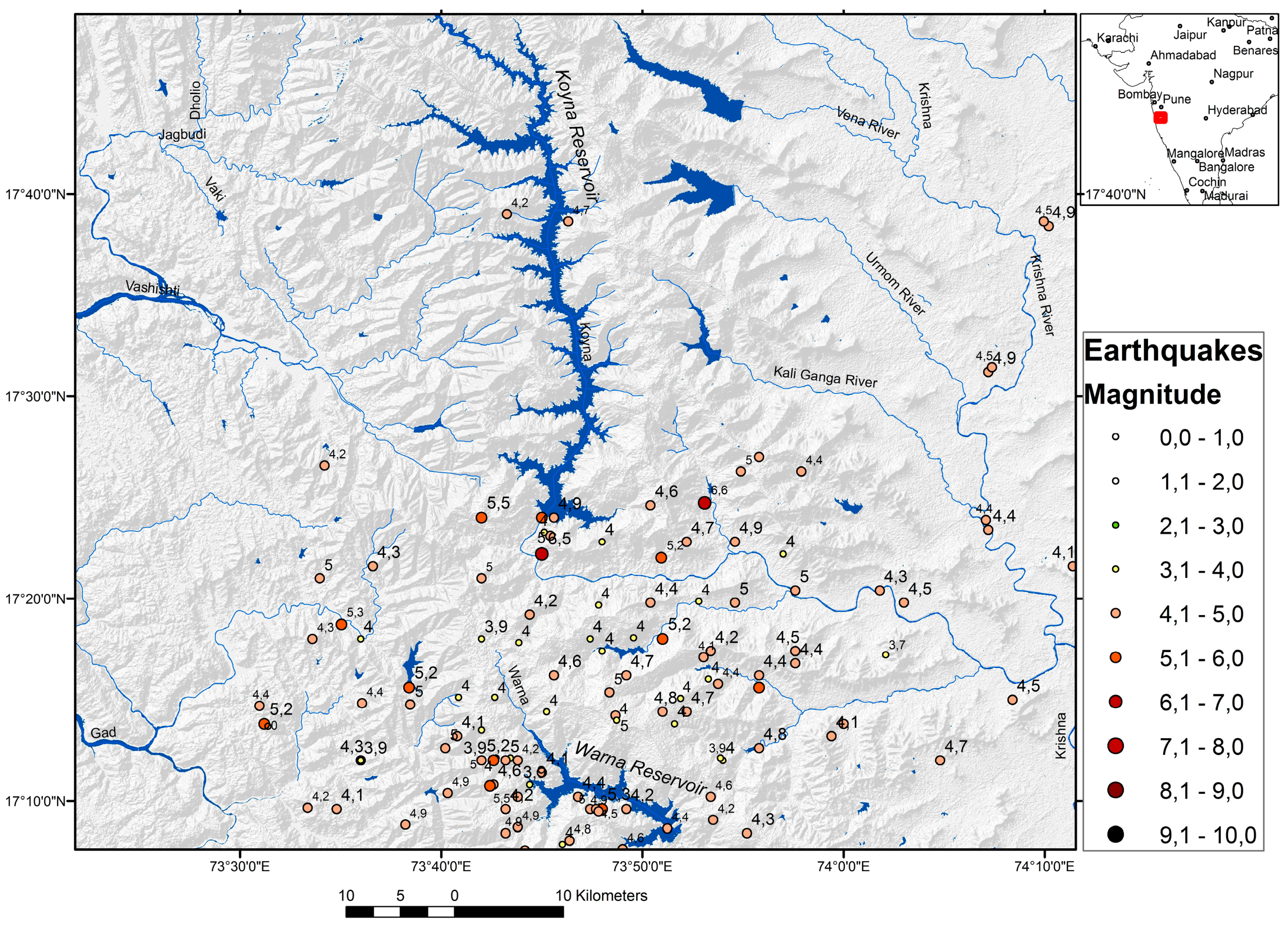
The Koyna region, situated in the western Deccan Plateau region of India, has been experiencing continuous seismicity since 1963 after the impoundment of the Koyna reservoir in 1961 (
Figure 1) [
1,
2]. The Koyna Dam is one of the largest dams in Maharashtra, India. The water input from the catchment of the Koyna River gave rise to Shivaji Sagar Lake, which is approximately 50 km in length [
3]. The strategic placement of the Koyna Dam reservoir and its social and financial importance make it necessary to undertake a thorough and complete study of natural hazards likely to impact this national facility.
The continuing seismic activity is related to reservoir loading that influences stressed faults [
4,
5,
6,
7], which was found to enhance with increased water damming, albeit with a short time lag [
8] and/or because the fluid pore pressure causes a shift in the underlying earth, leading to increased seismicity [
8,
9,
10]. The seismicity at the reservoir can be subdivided into mainly two types: the rapid response following immediately the reservoir impoundment as a direct effect of loading; and the delayed response occurring after a longer time. In the latter case, the seismicity seems to be correlated with a rapid increase in the water level. Type 1 seismicity is considered to be dominated by the elastic response to the reservoir load, while Type 2 is influenced more by pore pressure diffusion processes [
8].
Fluids act as major catalysts in earthquake generation processes. The central role of fluids in seismic faulting is known in all stages of the earthquake cycle, such as in the nucleation process, in the dynamic propagation and in the post-seismic evolution. Pore fluid pressure affects the whole earthquake process starting from fault nucleation. It continues through thermally-activated pressurization and mechanical lubrication and, finally, plays a role in triggering aftershocks [
9,
10,
11,
12]. Seasonal variations in seismic activity have been found in the Koyna region, which is seen to correlate with the seasonality of ground water recharge and precipitation [
12].
Pore pressure variations are considered to alter the strength of faults. If the faults are close enough to failure, then minor pressure variations as associated with precipitation can trigger earthquakes, even up to a few kilometers’ depth [
13]. The widely-accepted understanding is that an increase of the pore fluid pressure reduces the effective normal stress and, thus, the strength of faults, promoting earthquake rupture. However, the existence of deep reaching faults channeling the infiltration of precipitation can lead to significantly higher stress changes [
14,
15,
16,
17,
18].
Faults are typically characterized by higher permeabilities and low strength. Fluids migrate more easily along faults than through compact rocks. Thus, for different triggering mechanisms, such as an external fluid intrusion or local stress transfer, earthquakes are expected to occur preferably along pre-existing fault planes. Precipitation changes groundwater levels and simultaneously induces a slight redistribution in the stress and pressure regime near the faults as per the Mohr–Coulomb failure criterion [
14], thereby triggering earthquakes [
15,
16,
17,
18]. The time required for failure depends on factors, such as the load rate and remanent residual stress from previous earthquakes. In the study area, little is known of the surface water infiltration depth, directly from the reservoir itself, or the fluid infiltration depth downwards along the fault zones.
2. Objectives
Pore pressure diffusion is considered to play a key role in controlling the occurrence of earthquakes associated with Koyna and Warna reservoir [
8,
9,
10,
11,
12,
13,
14,
15,
16,
17,
18,
19]. Hence, the prevalent fault structure and tectonic setting in the region that influence seismicity need further investigation. The detailed inventory preparation of the near-surface fault and fracture pattern is likely to help detect relatively high permeable areas that allow intrusion and infiltration of surface water. Towards this end, satellite data were harnessed to detect near-surface fault and fracture zones and to understand the structural pattern via visual lineament analysis. The Sentinel satellite radar images available since 2015 from ESA are assumed to delineate sub-surface structures whose subtle morphological details are enhanced, which were earlier lacking in detail, due to radar backscatter of the surface. Landsat 8 data available since 2013 are also seen to show improvement when compared to previous Landsat missions because of enhanced radiometric and thermal resolutions. One of the goals of the present paper was to investigate whether additional structural/tectonic information can be gleaned from these newly-available satellite data.
The objective of this study was also to investigate the feasibility of visual lineament analysis to detect surficial traces of fracture and fault zones. These are sometimes seen to influence the contour and degree of seismic shock and intensity of secondary effects [
20,
21]. It must be noted that fault segments, their bends and intersections are more likely to concentrate stress and amplify seismic shock. Intersecting fault zones can cause constructive interference of multiple reflections of seismic waves at the boundaries with the surrounding rocks. Fault segments, especially of the en-echelon type, fault bends and fault intersections are probable sites o stress concentration and amplification of seismic shocks. The highest risk is seen to be concentrated along junctions of differently-oriented ruptures, especially at their intersections.
In the present attempt, meteorological data and water level changes, along with the tectonic inventory, were taken into account to comprehensively understand the triggered seismicity at Koyna where seasonal influences are seen to be prominent.
3. Geographic, Geologic and Seismotectonic Setting of the Koyna Area
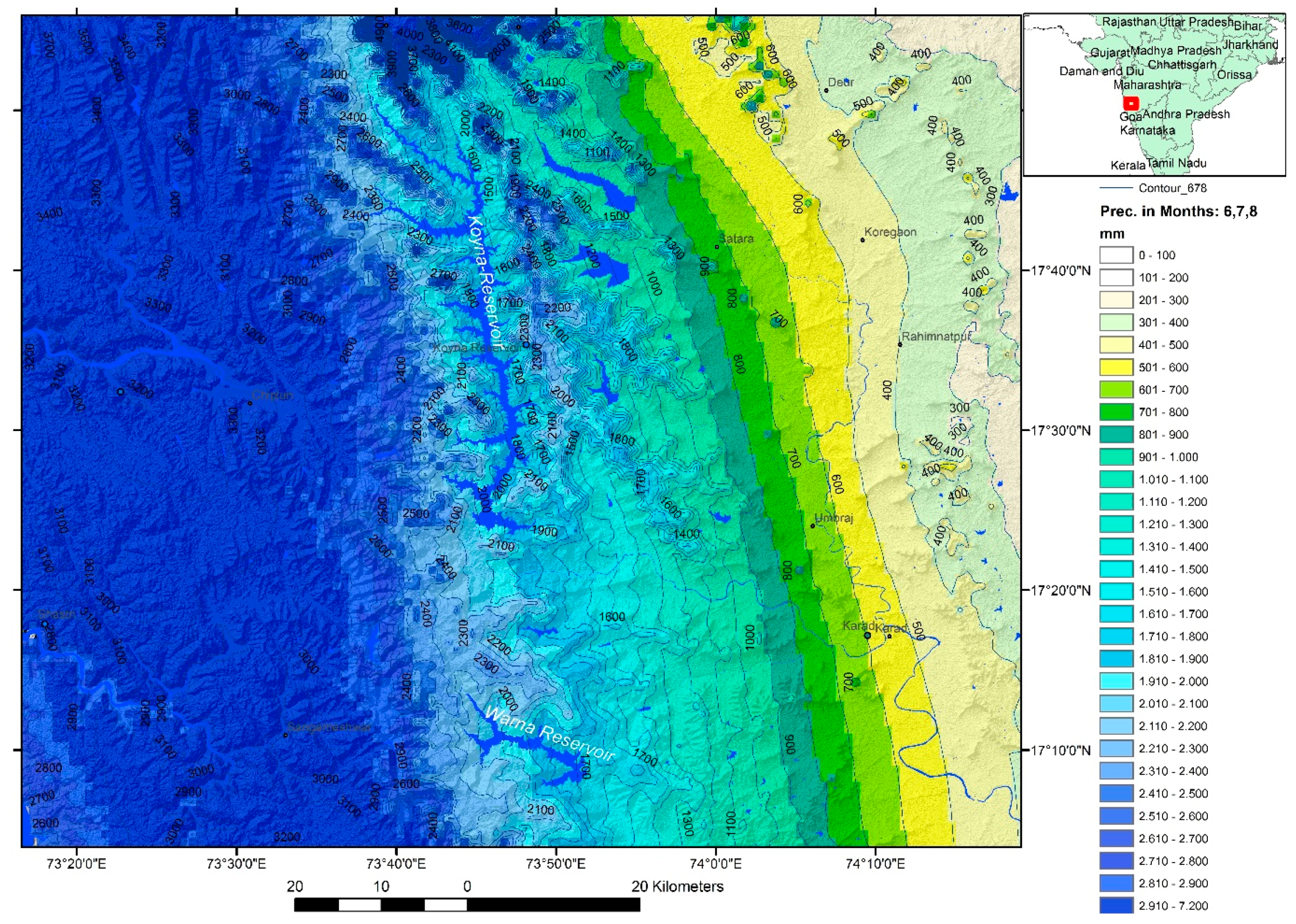
The Koyna reservoir, fed by the Koyna River, is situated on the elevated, north-south-trending Western Ghat escarpment, parallel to the west coast of India. The Koyna River has its origin near Mahabaleshwar and is a major tributary to Krishna. The defining feature of Koyna River is its NS flow direction with a north-south trajectory for almost 65 km. Most of the rivers in the neighborhood are seen to flow either east or west immediately after origin. The average precipitation in the study area ranges from 2500 to 3000 mm/year [
19]. The precipitation is more in the months between June and August (
Figure 2). Every year with the beginning of the monsoon, the water level rises in the reservoir. The increased water load probably influences the seismic activity with a time delay depending on the infiltration rate.
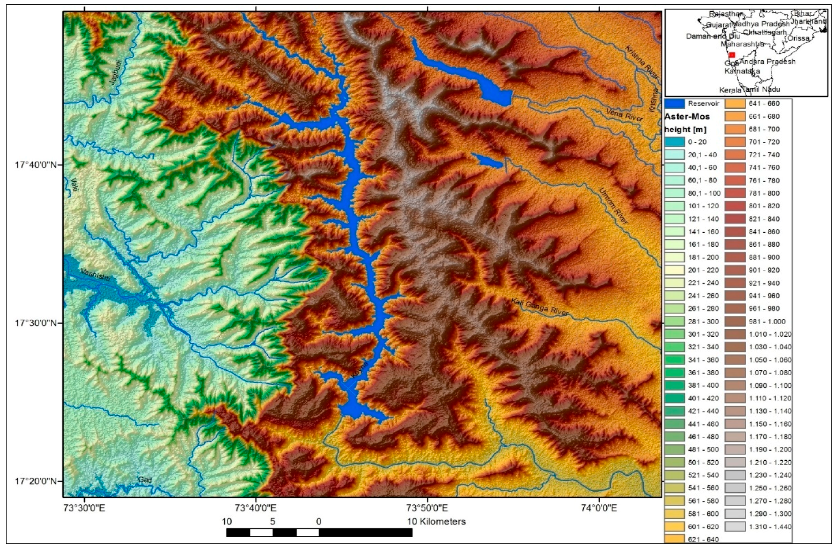
The mean elevation of the Western Ghats varies from about 600 m on the escarpment to about 100 m within the Konkan Plains to the west (
Figure 3). The escarpment is assumed to be fault derived and related to a zone of NNW to NE-trending en-echelon faults that parallel the coast [
8,
22,
23,
24,
25,
26].
The geological setting of the study region and its vicinity are characterized by the presence of Deccan Traps of 67.4 Ma comprising several sequences of lava flows. The Deccan Trap erupted during the separation of the Seychelles micro-continent from India, about 50–60 Ma [
27]. It encompasses different geologic and tectonic regimes and the westerly escarpment of India [
28]. The strain pattern in the study area seems to reflect the transmitted stress field due to Indo-Eurasian continental plate collision in the NS to NNS direction. The thickness of the Deccan Trap varies from 1.5 km in the escarpment zone to less than 100 m in the peninsular shield [
29]. The massive, compact lava sequences generally show low permeability, but there is significant migration of water through faults, fractures, columnar jointing or through vesicles. A review of the seismic history in the Koyna region, Patan Tahsil, shows this zone to be seismically active, though records of seismicity before 1963 are limited or non-existent. This region experienced many earthquakes that destroyed several buildings and caused severe casualties, particularly during the earthquake in 1967 with a macroseismic intensity of 10 and a magnitude of 7.3 [
30,
31,
32].
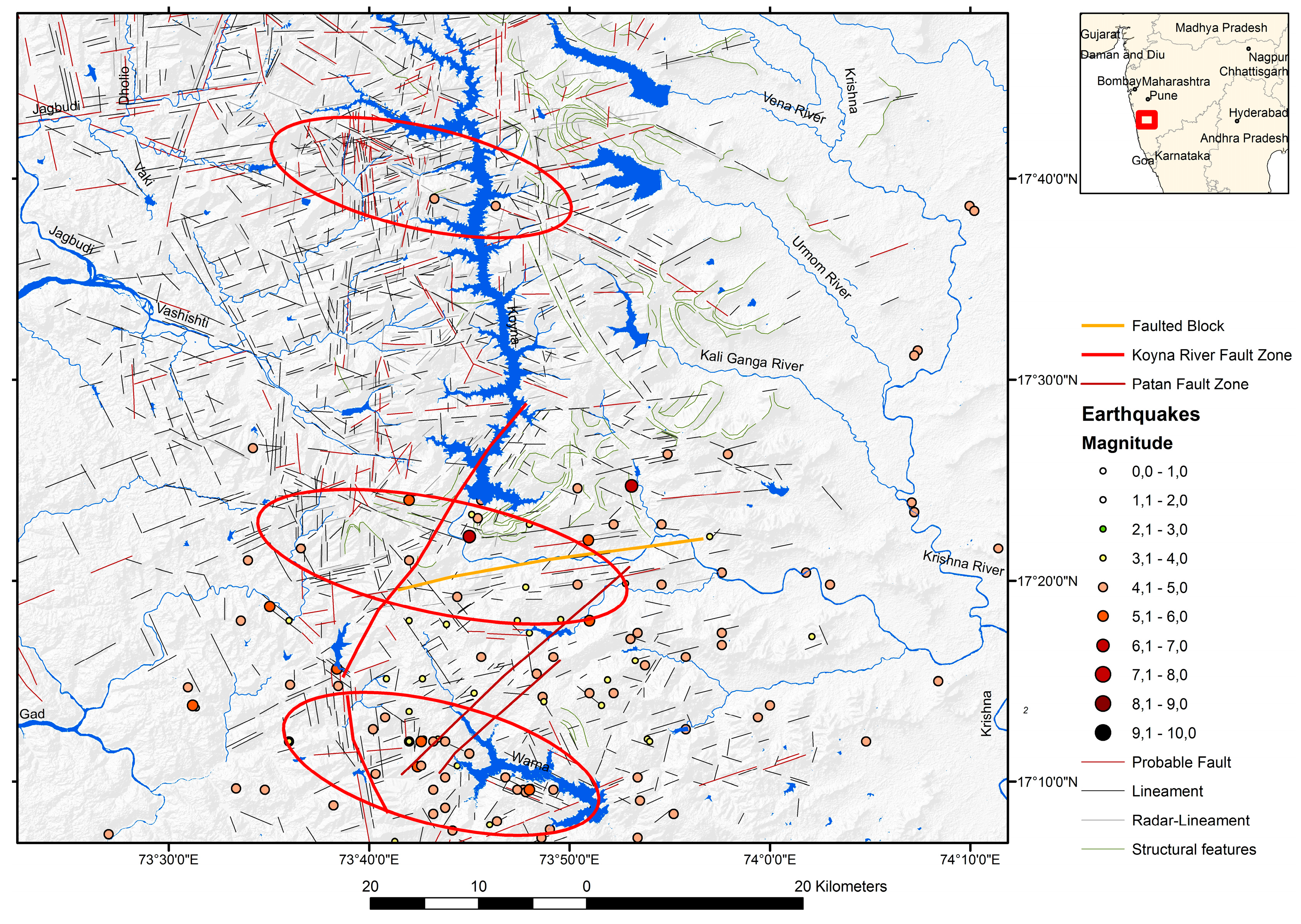
Gahalaut
et al. (2004) identified two major seismic zones referred to as the NNE-SSW-trending Koyna Seismic Zone (Koyna River Fault Zone (KRFZ)) and SSE-NNW direction Warna seismic zone (Koyna Faulted Block Zone) [
33]. The first is a broad NNE-SSW zone, which extends from north of the Koyna Dam and 40 km to its SSW direction.
The seismicity in the southern part of the reservoir is bounded in the west by the Koyna River Fault Zone (KRFZ) and in the east by NE-SW-trending Patan Fault. The area between the KRFZ and the Patan Fault is intersected by a number of NW-SE-trending fractures, which may be continuing from near the surface to the hypocentral depths and may act as conduits to the accumulation of fluid pressure [
34,
35].
The sub-basalt basement forms a local structural depression (pull-apart basin) caused by extension within the step-over zone between the right-lateral faults [
29] within which Koyna-Warna is situated. The right-lateral faults extend well beyond the immediate Koyna-Warna area. Sarma
et al. (2004) delineated the Koyna Fault Zone to be the weak expression of a moderately-conductive feature extending only up to a depth of 4–5 km [
36].
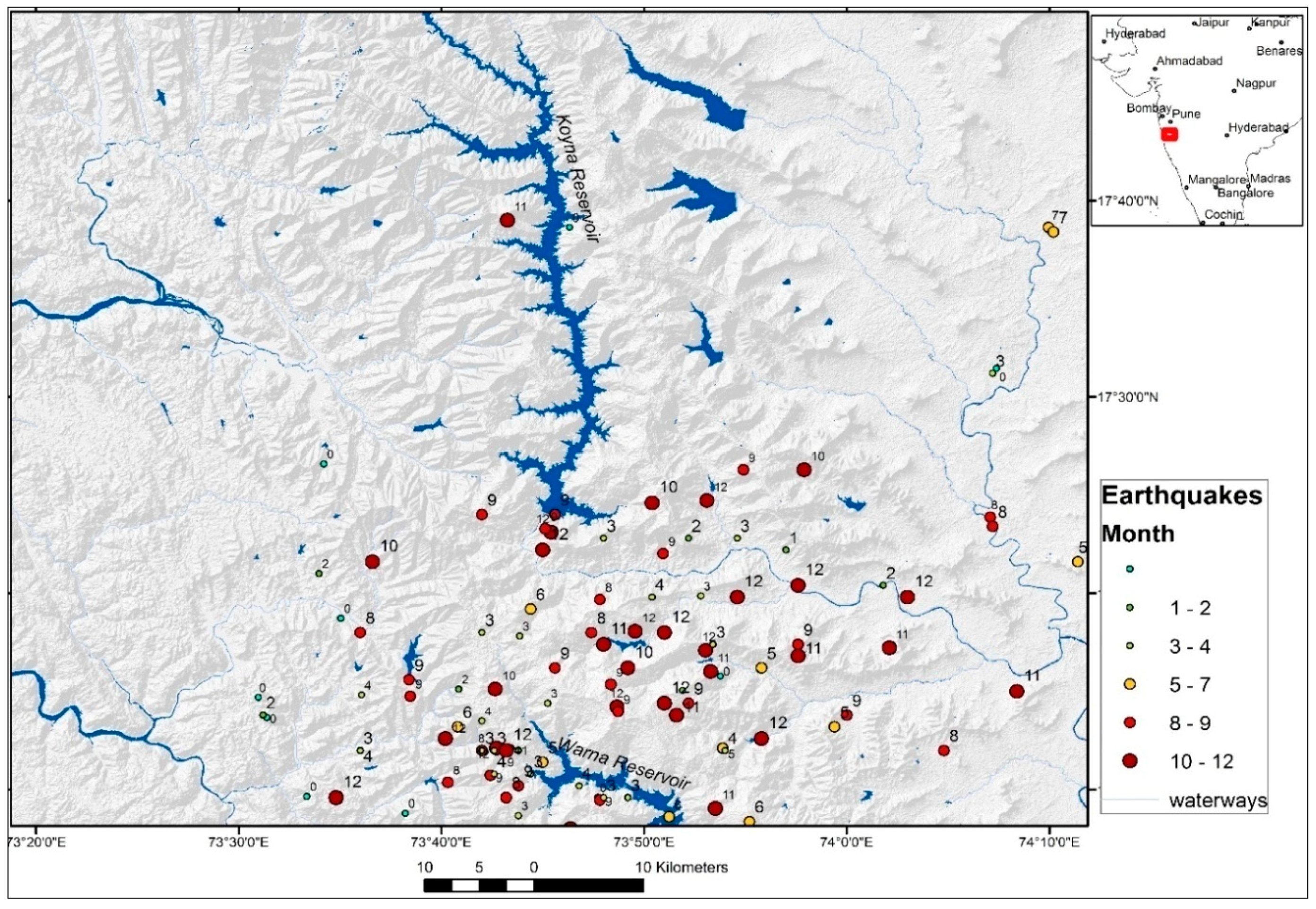
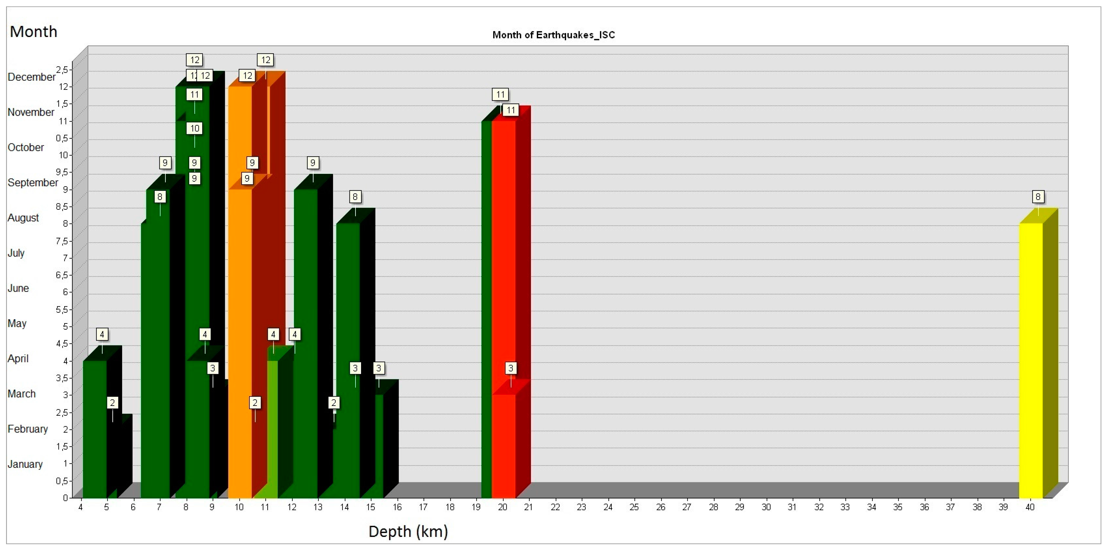
The incidence of earthquakes when compared to the month and depth (km) of their occurrence revealed that the bulk of them took place below a 10-km depth, after the humid months from June–September (
Figure 4 and
Figure 5). The majority of the earthquakes are seen to be concentrated in the post-monsoon period when the impounded water was at its maximum. Many of the earthquakes below a 10-km depth occurred in the months of November and December, implying a time delay between the surface water infiltration along the major fault and fracture zones and earthquake triggering effects. This suggests bends and fault step-over serve as an ideal tectonic environment for generating moderate–large magnitude-induced (reservoir, injection,
etc.) earthquakes.
4. Materials and Methods
Satellite Remote Sensing (RS) data and Geographical Information System (GIS) software have a huge potential and wide application in assessing and categorizing natural hazards [
37,
38,
39,
40]. GIS integrated remote sensing data and geospatial analysis can be used to infer factors related to the occurrence of major earthquake shocks and/or earthquake-induced secondary effects. The secondary factors include lithology (loose, unconsolidated sedimentary cover), faults, steeper slopes (landslide susceptibility) or areas with a higher groundwater table [
39].
Special attention was given to precise mapping of traces of tectonic patterns visible on satellite imagery, predominantly in areas with distinct linear features (tonal linear anomalies, geomorphologic linear features, etc.). The visibility of linear features depends on specific properties of satellite systems, such as their spatial and radiometric resolution or acquisition time. Lineament analysis was carried out based on Landsat and Sentinel radar imagery and on morphometric maps derived from digital elevation data, such as the Shuttle Radar Topography Mission (SRTM) and Advanced Spaceborne Thermal Emission and Reflection Radiometer (ASTER) Global Digital Elevation Model (GDEM) data.
The combined evaluation of structural field configuration, seismotectonic morphology and lineament analysis from RS has been carried out for decades in many earthquake-prone countries. Satellite RS data, enhanced with image processing techniques, can provide a synoptic view of long linear features saving on cost and time expended on field investigations. Long linear features identified on satellite images are related often to faults and lineaments after ruling out cultural noise, like drainage or roads.
Since lineament mapping is a very important component of this research, a short introduction can be useful for those not familiar with this methodology. The term lineament is a neutral term for all linear, rectilinear or slightly bent images, which are often expressed as scarps, linear valleys, narrow depressions, linear zones of abundant watering, drainage network, peculiar vegetation, landscape and geologic anomalies [
39,
41,
42]. Lineaments represent, in many cases, the surface expression of faults, fractures or lithologic discontinuities. In the present study, any linear arrangement of pixels depicting the same color/gray tone was considered to be a lineament. The emphasis was laid on lineament mapping, because it can contribute to: (1) developing the inventory and analysis of faults and fracture patterns relevant to surface water infiltration and rock permeability; (2) detecting subsurface influence on macro-seismic intensity; and (3) inferring the subsurface, structural influence on earthquake-induced secondary effects, such as slope failure. The visibility of linear features depends on specific properties of satellite systems, such as their spatial and radiometric resolution or acquisition time [
41,
42].
It is often difficult to identify faults and lineaments in the field, because of a plethora of geological conditions, like sedimentary cover, erosion, vegetation over-growth, scale and other factors, including the experience of the geologist or prohibitive costs for manned surveys. Accessibility is also another limiting factor. Because of all of these shortcomings, RS data are a valid source for getting accurate information of Earth surface features and land use/land cover patterns.
Linear features, in the present study, were enhanced by merging processed satellite data with filter tools using Landsat RGB / false composite imagery. The mapped lineaments were then compared to seismotectonic data, mainly with the position of earthquake epicenters, the months of occurrence and depth. Special attention was focused on precise mapping of traces of faults (linear anomalies in the drainage pattern, in the morphology or within outcropping rocks) on satellite imagery, predominantly in areas with distinct expressed lineaments, as well as in areas with intersecting/overlapping lineaments.
4.1. Evaluation of Landsat-Data
Landsat data, available freely from the U.S. Geological Survey, EarthExplorer [
43] and Global Land Cover Facility (GLCF) University of Maryland, USA [
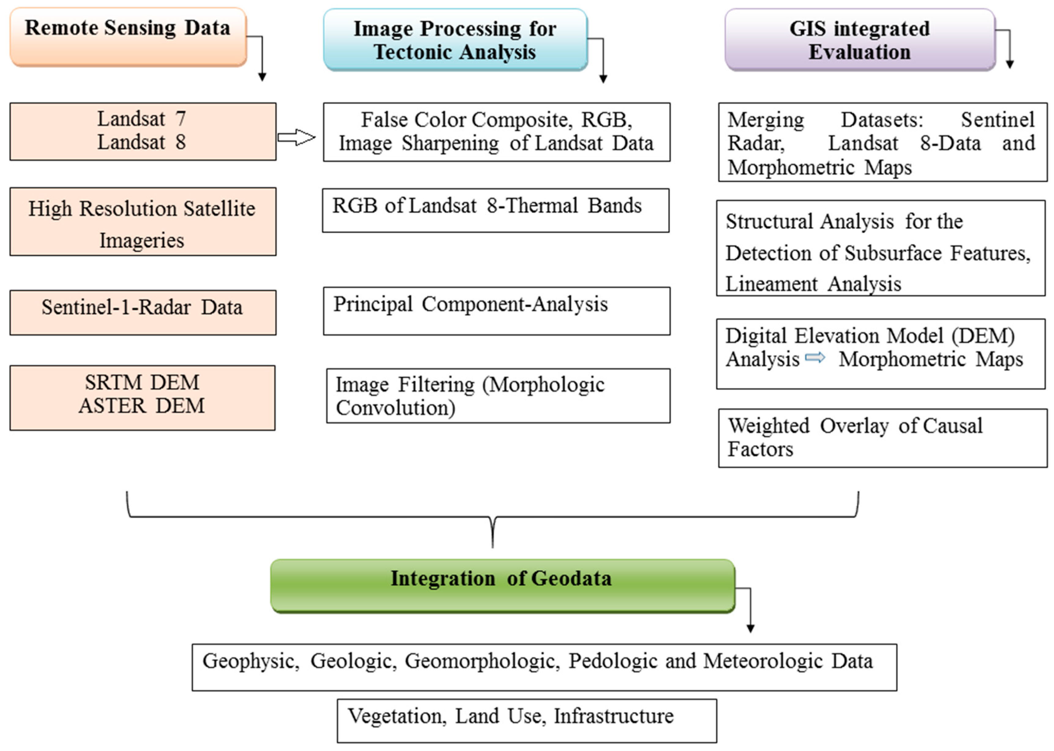
44], were used in the present study. The Landsat images were digitally processed using image processing and GIS software to improve the appearance of the imagery and to assist in visual interpretation and analysis. The chosen image processing was mainly directed to detect surface traces of faults and fracture zones. Examples of enhancement function include contrast stretching to increase the tonal distinction between features in a scene and spatial filtering to enhance specific spatial patterns in an image. The flow chart is presented in
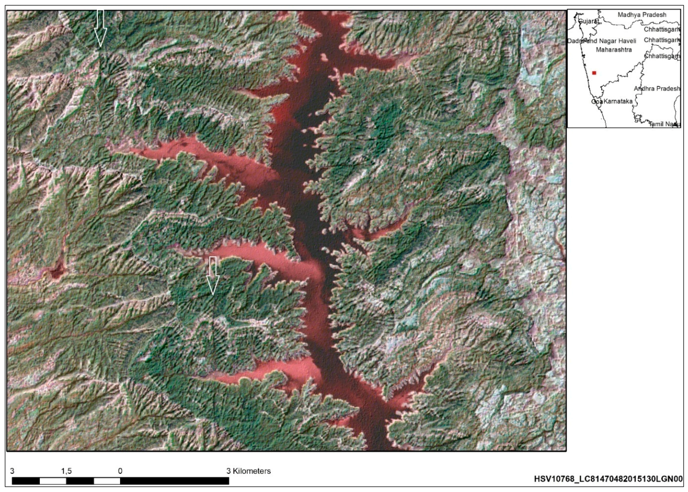
Figure 6. Based on satellite data, false color composites were created according to the Red, Green, Blue (RGB) approach. The chosen band combinations were determined by the objectives of this study.
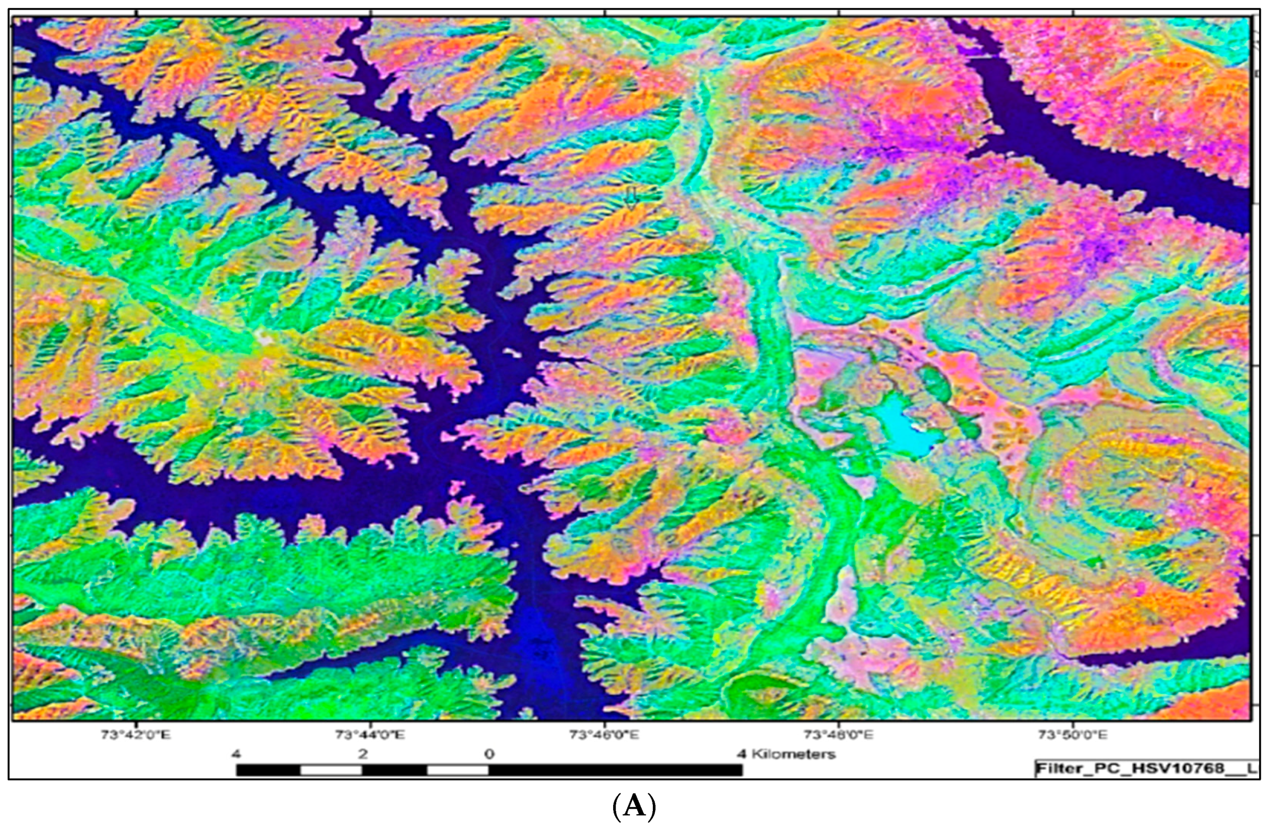
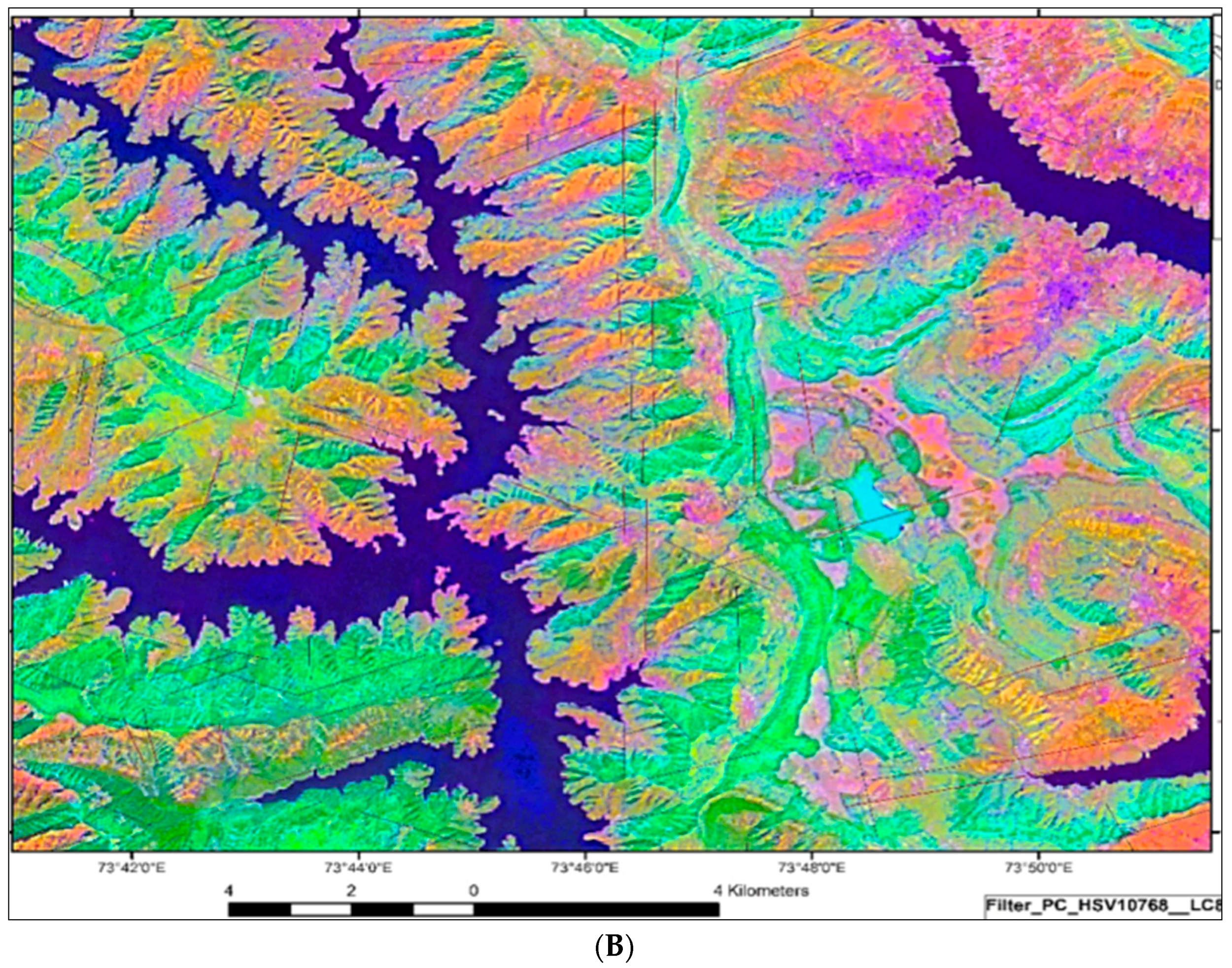
The RGB principle is reviewed briefly: Three images from the different Landsat bands are used as end-members in a triplet, in which each image is given a particular false color for a False Color Composite (FCC). In principle, any image can be coded in any color. Histogram stretching has been used to increase the intensity and sharpness of the images prior to FCC enhancements. The thermal channels, combined in RGB images of Landsat 8, allow better visibility of tonal, linear anomalies due to different thermal emissivities. Low pass and high pass filters and directional variations were used to detect subtle surface structures, such as linear escarpments. By merging the “morphologic” image products derived from the “Morphologic Convolution” image processing in ENVI software (directional filter, kernel size 3 × 3) with RGB imageries, the evaluation feasibilities were improved. Vegetation index imageries were also used to detect linear anomalies. Unsupervised and supervised image classifications served as a base for land use/cover mapping, such as forests, wetlands and fields. Principal Component Analysis (PCA) of the Landsat 8-RGB images revealed structural information, as well.
4.2. Sentinel-Radar Data
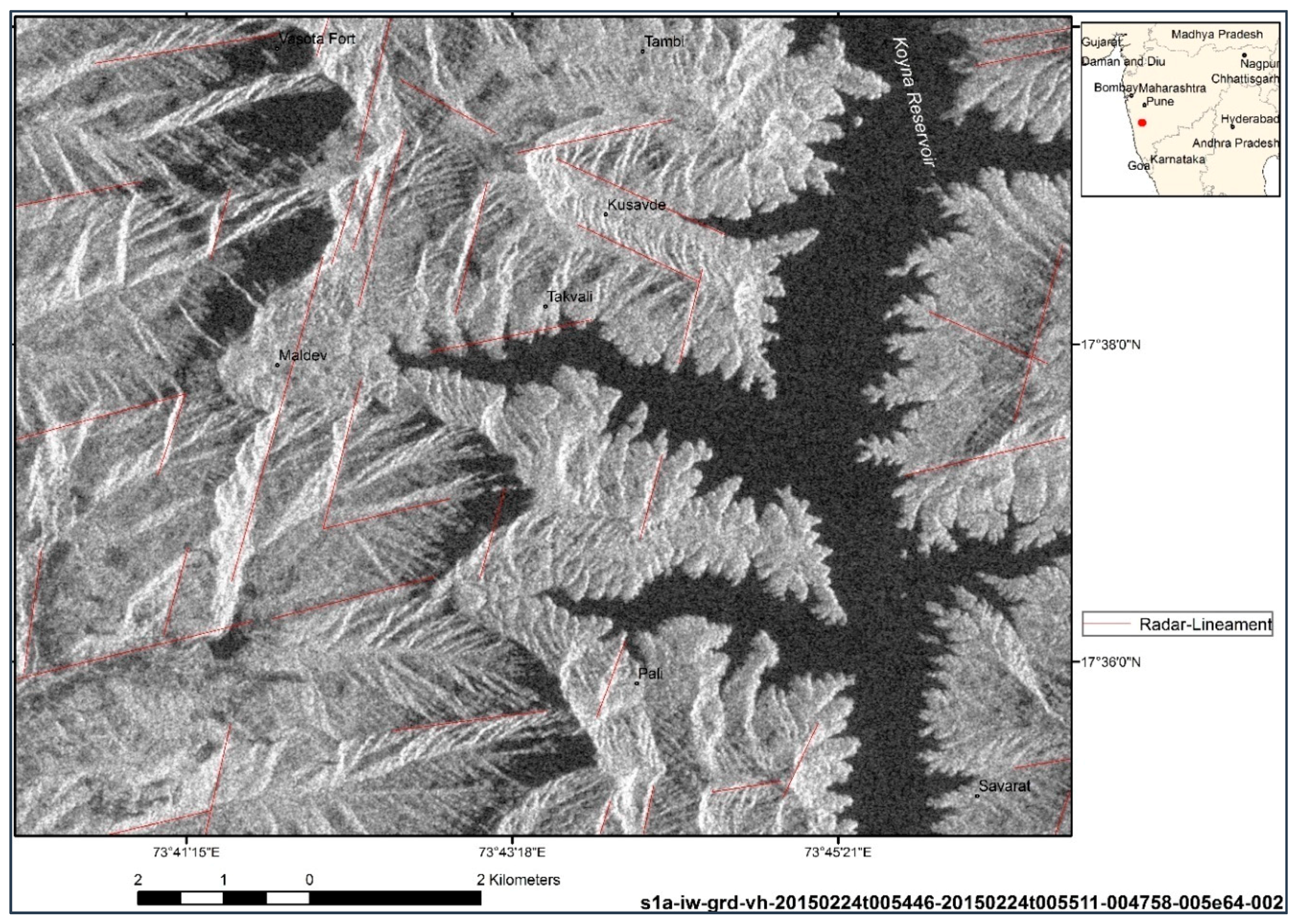
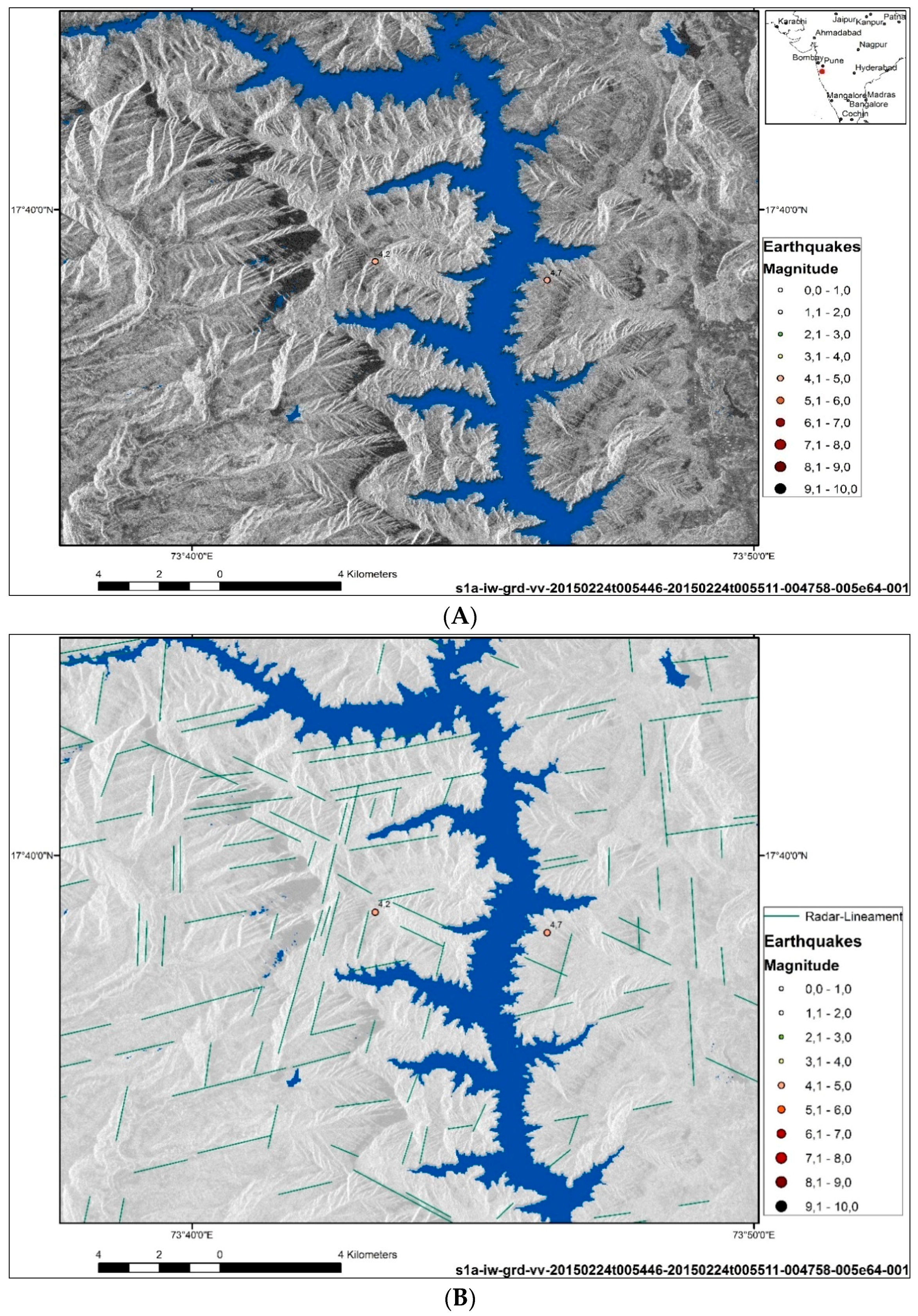
Sentinel radar images of the Koyna area available since October 2014 were included in the investigations. The satellite radar data are provided by the Sentinel-1 mission, a joint initiative of the European Commission (EC) and the European Space Agency (ESA) [
45]. The Sentinel-1 mission contains C-band imaging, operating in four exclusive imaging modes with different resolutions (down to 5 m) and coverage (up to 400 km). Although radar foreshortening and lay-over effects have to be considered in the Koyna area, linear, tonal features appear on the radar images, which are probably related to traces of sub-surface structures (
Figure 7). These linear features were mapped as “radar lineaments”.
4.3. Analysis of Digital Elevation Model Data
Based on DEM data, morphometric maps, such as shaded relief, aspect and slope degree, minimum and maximum curvature or plan convexity maps using ENVI and ArcGIS software were created. Morphometric maps, such as slope, hill shade, height level and curvature maps, were generated based on the SRTM and ASTER GDEM Digital Elevation Model (DEM, 30-m spatial resolution) data using ArcGIS/ESRI and ENVI/EXELIS digital image processing software. The Shuttle Radar Topography Mission (SRTM) obtained digital elevation data to generate a high-resolution digital topographic database. SRTM was an international project spearheaded by the National Geospatial-Intelligence Agency (NGA), NASA, the Italian Space Agency (ASI) and the German Aerospace Center. Similarly, the Ministry of Economy, Trade and Industry (METI) of Japan and the United States National Aeronautics and Space Administration (NASA) jointly released ASTER GDEM.
GIS-integrated geospatial geodata analysis can be used to detect, map and visualize factors that are known to be related to the occurrence of higher earthquake shocks and/or earthquake-induced topography, fault zones or steeper slopes.
Morphometric properties of an area can influence to a great deal local site effects during earthquakes and earthquake-related secondary effects. When searching for areas susceptible to soil amplification, liquefaction or compaction, the so-called causative or preparatory factors have to be taken into account. These include height level, slope gradient, terrain curvature, lithologic conditions and fault zones. Morphometric factors can be extracted from DEM data that might be of importance for the detection of local site conditions influencing earthquake ground motion: Height level maps help to search for topographic depressions covered by almost recently-formed sediments, which are usually linked with higher groundwater tables. Extracting the lowest height level of an area makes visible areas with high groundwater tables. In case of stronger earthquakes, such areas have often shown the highest earthquake damage intensity, compaction and liquefaction occurrence. From the DEM data, flat areas with no curvature of the terrain and low to no slope gradients were extracted.
SRTM and ASTER GDEM data-derived morphometric maps (slope gradient maps, drainage, etc.) were combined with lithologic and seismotectonic information in a GIS database.
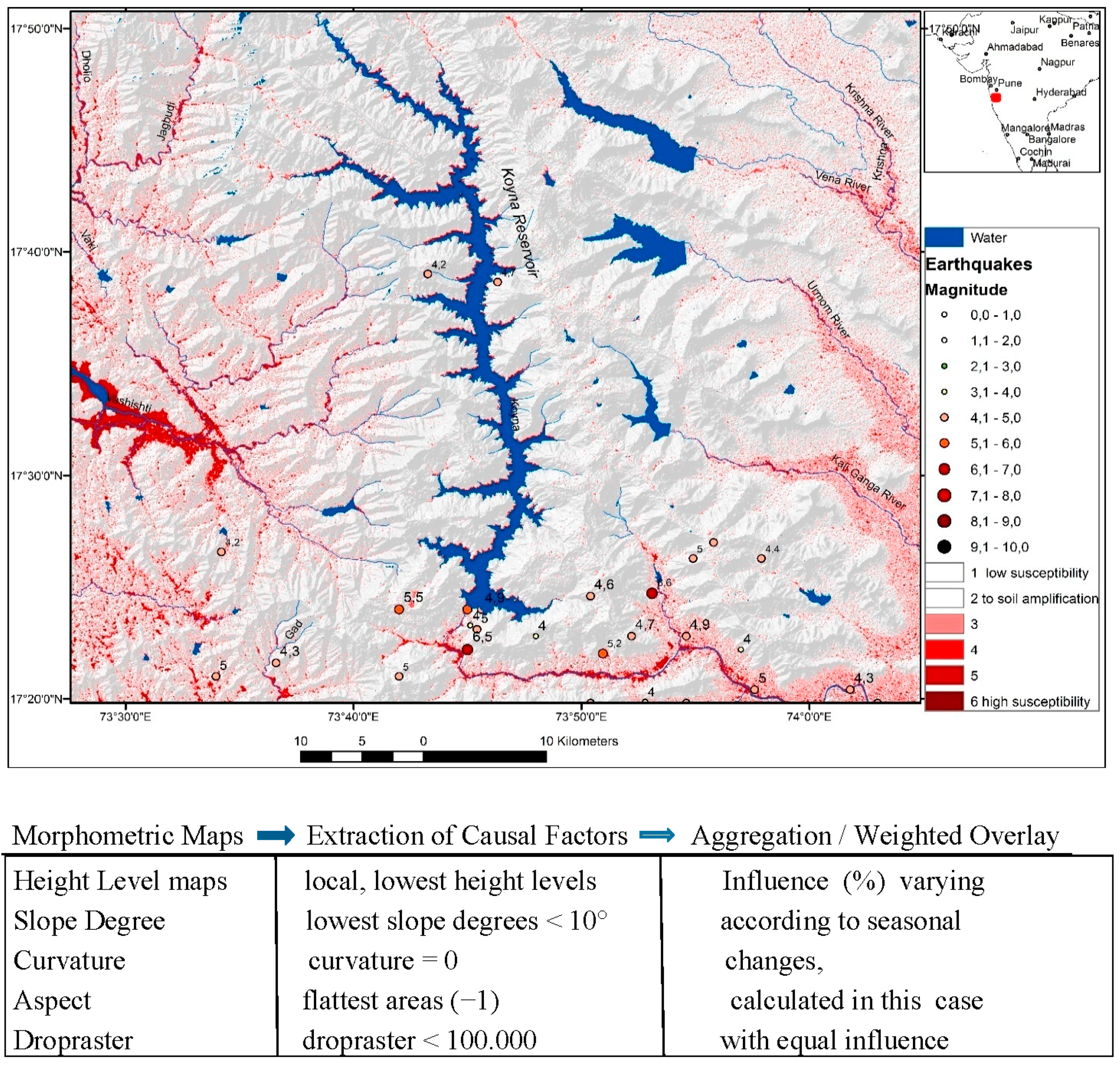
An important step towards susceptibility mapping is the weighted overlay method in ArcGIS. The influence of the factors on earthquake ground motion is not equally important in the analysis. The percentage of influence of one factor might be changing, for example due to seasonal and climatic reasons or distance to the earthquake source. As a stronger earthquake during a wet season will probably cause more secondary effects than during a dry season, the percentage of its influence has to be adopted. In very hot and dry seasons, the risk of liquefaction or landslides is generally lower than in humid seasons. The sum of all factors/layers that can be included in the GIS provides information of the susceptibility to amplify seismic signals. The analysis method and integration rules can easily be modified in the GIS architecture as soon as additional information becomes available [
42].
The causative, morphometric factors, such as the lowest local height level, slope degrees <10°, curvature = 0 (negative curvature represents concave, zero curvature represents flat and positive curvature represents convex landscape), drop raster <100,000, were aggregated and, in this case, weighted with equal influence. The drop raster was created using the Hydrology tools of ArcGIS (the drop raster is calculated as the difference in
z-value divided by the path length between the cell centers, expressed as percentages) [
39,
41,
42]. An overview of the areas assumed more susceptible to earthquake ground motion due to their morphometric properties is shown in
Figure 8. The dark red areas in
Figure 8 are considered to be more susceptible to soil amplification. This is because of the presence of relatively higher groundwater tables in the lowest parts of the valley bottoms; flat morphology with low slope and curvature gradients; and unconsolidated, sedimentary covers. Comparing the results of the weighted overlay calculations with geologic maps, there is a clearly visible coincidence of areas with higher susceptibility values and the outcrop of unconsolidated, quaternary sediments in the broader valleys and depressions. When underlain by larger fault zones, the soil amplification susceptibility will probably rise, depending on the earthquake properties and parameters, such as depth, magnitude and orientation of the fault plane solution.
4.4. Evaluation of Shear Wave Velocity Data
Local site conditions are detected by different methods. To provide a first approximation of these conditions, an approach was developed to characterize potential ground motions based on known correlations between variations in shear-wave velocity and topographically-distinctive landforms by applying geomorphometry, a quantitative description of landforms based on DEMs . Wald and Allen (2009) described a methodology for deriving maps of seismic site conditions using topographic slope as a proxy [
46,
47,
48]. V
s30 measurements (the average shear-velocity down to 30 m) were correlated against topographic slope. They also favorably compared topographic slope-based V
s30 maps with existing site condition maps based on geology. We converted the V
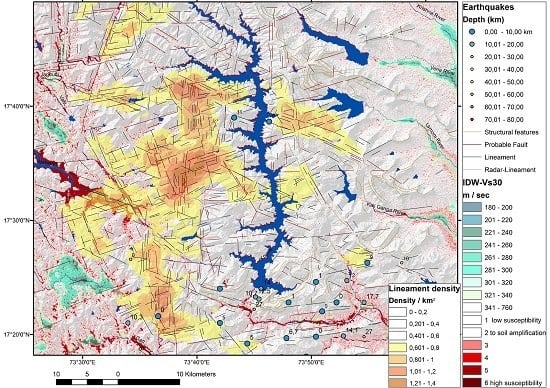
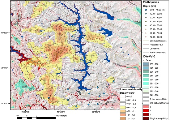
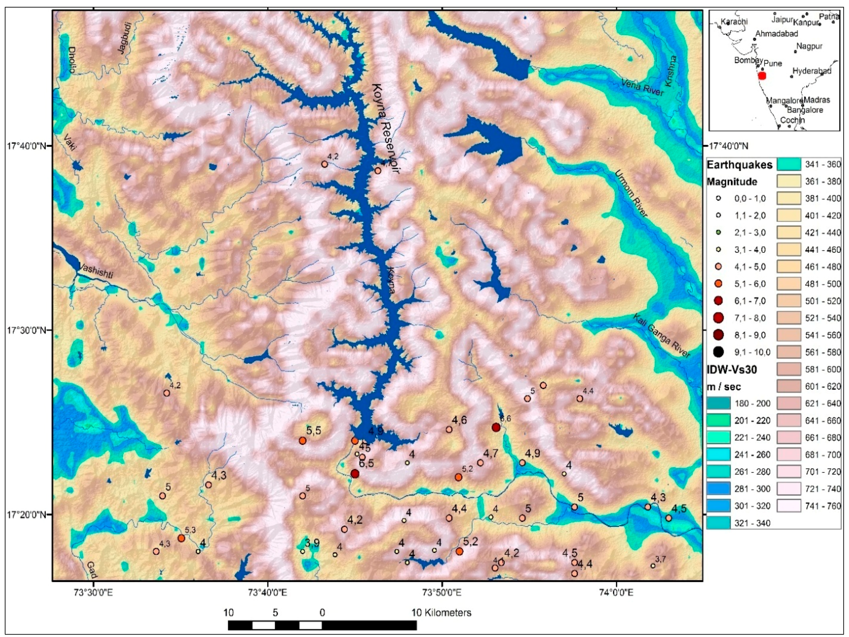
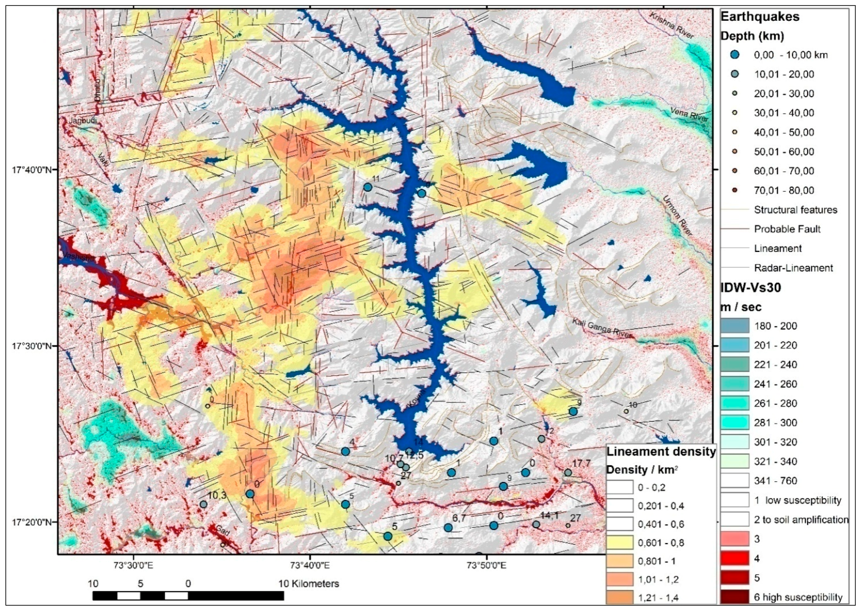
s30 data into point-shape files, which served as a base for IDW (Inverse Distance Weighted) interpolations (
Figure 9). The resulting interpolation maps were overlain then with geologic and morphometric maps.
To derive
Figure 9, V
s30 data acquired from USGS were used with the assumption that lower V
s30 values contribute to higher earthquake damage. This assumption was confirmed by previous investigations in other areas such as in Morocco [
20]. However, this assumption can lead to errors as well due to, for example, faulty DEM data or by flat areas not related to young, unconsolidated covers, such as extensive erosion surfaces (peneplains). Therefore, a careful and accurate comparison with the geologic and geomorphologic conditions in the investigation area is necessary.
The reservoir area is characterized by estimated Vs30 data ranging between 600 and 760 m/s. The dam site area is obviously not affected by higher susceptibility to soil amplification, as in the case of lower Vs30 velocities (<400 m/s) within broader valleys and depressions.
6. Conclusions
There is a strong need to create and improve the systematic and standardized inventory of areas like Koyna that are susceptible to seismic hazards. These hazards can be amplified by local site conditions pertaining to higher ground motions or can be related to secondary effects, such as landslides, liquefaction or compaction. The present study has demonstrated the feasibility of remote sensing and GIS creating a basic, yet standardized dataset, with relatively low financial resources. By using open-source data and web gateways to acquire comprehensive geologic, geophysic and geomorphologic information that influences local site conditions in the case of stronger earthquakes.
The present study has shown that the Koyna reservoir area is nearly not affected by soil amplification due to local site conditions because of morphometric and lithologic site properties. However, the study has also thrown up some issues pertaining to the influence of ongoing tectonic movements along fault zones, the impact of fluids along these fault zones or the possible amplification of seismic waves along fault zones acting as seismic reflectors, impacting the seismic risk of the reservoir area. To resolve these questions, detailed field research needs to be carried out.
In the near future more Sentinel radar images will be available from ESA with different acquisition times and illumination geometries. These should be continuously evaluated and integrated into the existing database, adding to the refining of the tectonic pattern of this area. Satellite imagery can serve as a georeferenced base for mapping linear features related to subsurface structures, thus contributing to the structural inventory. GIS-integrated evaluations of different satellite data have contributed to the detection of subsurface structures in the Koyna area. It has also delineated areas prone to potential damage.
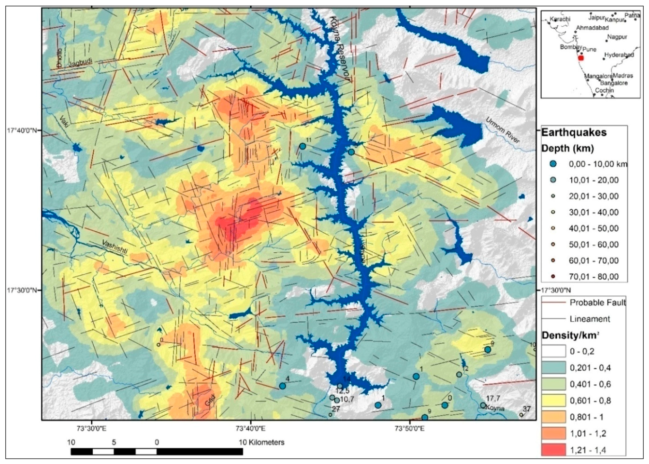
Areas with a relatively higher lineament density provide hints where the intrusion and infiltration of surface water into the subsurface might be more intense due to fracture zones within the outcropping rocks.


