Shallow Shear-Wave Velocity Beneath Jakarta, Indonesia Revealed by Body-Wave Polarization Analysis


1
Research School of Earth Sciences, Australian National University, Canberra, Australian Capital Territory 0200, Australia
2
Global Geophysics Research Group, Institute Teknologi Bandung, Bandung 40116, Indonesia
3
Geoscience Australia, Canberra, ACT 2609, Australia
*
Author to whom correspondence should be addressed.
Geosciences 2019, 9(9), 386; https://0-doi-org.brum.beds.ac.uk/10.3390/geosciences9090386
Submission received: 28 June 2019
/
Revised: 10 August 2019
/
Accepted: 30 August 2019
/
Published: 3 September 2019
(This article belongs to the Special Issue Inaugural Section Special Issue: Key Topics and Future Perspectives in Natural Hazards Research)
Abstract
:Noting the importance of evaluating near-surface geology in earthquake risk assessment, we explored the application to the Jakarta Basin of a relatively new and simple technique to map shallow seismic structure using body-wave polarization. The polarization directions of P-waves are sensitive to shear-wave velocities (Vs), while those of S-waves are sensitive to both body-wave velocities. Two dense, temporary broadband seismic networks covering Jakarta city and its vicinity were operated for several months, firstly, from October 2013 to February 2014 consisting of 96 stations, and secondly, between April and October 2018 consisting of 143 stations. By applying the polarization technique to earthquake signals recorded during these deployments, the apparent half-space shear-wave velocity (Vsahs) beneath each station is obtained, providing spatially dense coverage of the sedimentary deposits and the edge of the basin. The results showed that spatial variations in Vsahs obtained from polarization analysis are compatible with previous studies, and appear to reflect the average Vs of the top 150 m. The low Vs that characterizes sedimentary deposits dominates most of the area of Jakarta, and mainly reaches the outer part of its administrative margin to the southwest, more than 10 km away. Further study is required to obtain a complete geometry of the Jakarta Basin. In agreement with previous studies, we found that the polarization technique was indeed a simple and effective method for estimating near-surface Vs that can be implemented at very low-cost wherever three-component seismometers are operated, and it provides an alternative to the use of borehole and active source surveys for such measurements. However, we also found that for deep basins such as Jakarta, care must be taken in choosing window lengths to avoid contamination of basement converted phases.
1. Introduction
The growth of the global population over the past century, combined with the accelerating pace of urbanization, has resulted in the explosive growth in the number of megacities (population over 10 million). Especially in the developing world, many of the buildings in these cities have not adhered to earthquake resilient construction practice with the result that “an epicentral hit on a megacity has the potential to cause 1 million fatalities” [1]. Also, many of these cities are concentrated in sedimentary basins, because of their flat topography and access to fertile soils, sources of water and maritime commerce. Improving earthquake risk assessment is one of the most important ways of alerting policymakers to the danger earthquakes pose. This requires not only knowledge of the population and building exposure and “hard rock” seismic hazard, but also an understanding of the potential for sedimentary basins to cause amplification and resonance of seismic wave motion. The observation of such effects in recent destructive earthquakes—the 2015 Kathmandu [2] and 2017 Mexico City earthquakes [3]—imparts some urgency to the evaluation of basin effects in other megacities. Such an evaluation can be conducted by profiling the shear-wave velocity (Vs) of sedimentary deposits down to bedrock.
Many approaches have been developed to estimate Vs depth profiles based on geotechnical and geophysical methods. Direct approaches such as borehole drilling, vertical seismic profiling (VSP), and standard penetration testing (SPT) can give accurate information on the velocity profile. However, these are often too expensive to cover the entire area of a large city. Other approaches exist such as seismic refraction or reflection surveys, but these use active sources like explosives and require large, regularly-spaced sensor arrays that are impractical in built-up urban areas. These problems are avoided using passive approaches such as microtremor measurements [4,5,6,7] and interferometry studies [8,9,10,11], which have become very popular for use in densely-populated areas.
Recently, Park and Ishii [12] introduced an alternative approach for estimating “near-surface” Vs by using measurements of body-wave polarization. The term polarization is used here to address the wave’s particle motion (below we explain that “near-surface” Vs is actually apparent half-space Vs, which we denote as Vsahs). They utilized the well-known relationships between the Vs and compressional-wave velocity (Vp), and the polarization of body waves interacting with the free surface of a half-space. The incoming polarization directions of P-waves are sensitive to Vs, while those of S-waves are sensitive to both Vp and Vs. Therefore, it is possible to estimate near-surface Vs and Vp by observing the polarization directions of P-waves and S-waves generated by earthquakes at a seismic station. This approach requires no artificial source or other expensive equipment, and it can be applied with a minimum of computational effort.
Park and Ishii [12] concluded that their technique could be used very widely to study near-surface velocity structure wherever three-component seismometers are deployed. Since it is applicable to urban areas, we applied this technique based on P-waves polarization to map shallow Vs beneath Jakarta, the capital city of Indonesia. Because it lies on a thick young sedimentary basin [13,14,15,16], seismic risk in Jakarta is likely to be enhanced by amplification and resonance effects. In late 2013 and again in 2018, two temporary seismic networks consisting of three-component broadband seismometers were deployed for approximately 3 months and 5 months, respectively, covering most of the city and its vicinity. While Park and Ishii [12] presented their application using the Hi-net array in Japan, the combination of seismicity, dense seismic network, and sedimentary basin structure in Jakarta provides a good opportunity to evaluate this technique on a more local scale. The results are benchmarked against borehole data and shallow Vs estimated from other studies.
2. Geologic Setting and Seismometer Deployments
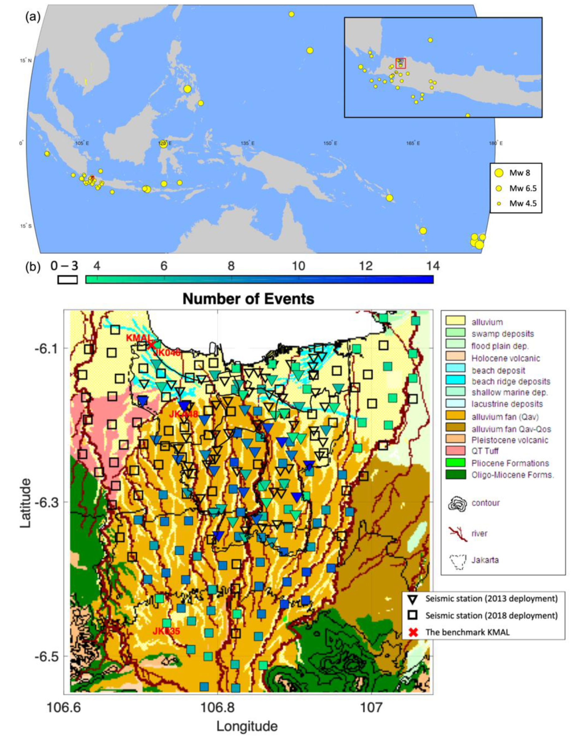
Located on the northern coast of the island of Java, the surface geology of Jakarta mainly consists of alluvial deposits. According to Turkandi et al. [17], the city’s surface geology from the coastline to around 6 km southward to the center of the city consists of Holocene sand dunes and alluvial fan, while deposits of Pleistocene alluvial fan cover the southern part of the city with little trace of Tertiary volcanic deposits. The sedimentary deposits are estimated to thicken northward, with alluvial fan sediments reaching thicknesses of 300 m or more in the city center. Unfortunately, although the geological setting of Indonesia is described generally in Van-Bemmelen [18], there are only a few recent studies of the detailed geological setting of the Jakarta Basin (e.g., Turkandi et al. [17]).
Nevertheless, the existence of a thick sedimentary basin overlying tertiary bedrock strongly suggests that amplification and resonance could enhance the damaging effects of earthquakes. After seismic waves propagate through the transition between stiff rock and soft soil, their energy is trapped within the soil layer by internal reflections [19]. The reverberating seismic waves add constructively at certain frequencies but interfere destructively at others, with the former being resonant frequencies that are determined by the thickness and Vs of the sedimentary layer. Because of resonance, the energy and amplitude of seismic waves, which normally decay rapidly in intensity with distance from the earthquake, can instead increase dramatically in both amplitude and duration. Not accounting for such basin resonances may lead to an underrated earthquake risk assessment.
To better understand such basin effects, three-component broadband seismometers (Trillium Compact) and digitizers built by the Australian National University were installed at various sites (Figure 1) in two separate deployments. Stations spaced at 3–5 km, were deployed temporarily on a concrete slab floor in schools throughout the city. The first deployment comprised 96 stations and operated from October 2013 to February 2014, covering most of the area of Jakarta. Twenty-six stations were maintained for 3 months of recording as semi-permanent stations and the other 26 stations were redeployed in three phases, each of one-month duration. The second deployment, comprising 143 stations was deployed in 2018 and aims to include coverage just outside Jakarta in order to reveal the extent of the basin edge. The 30 stations were maintained and redeployed in five phases with at least one-month duration for every site.
Using data from the first deployment, Saygin et al. [15] extracted Rayleigh wave Green’s functions from cross-correlograms of ambient noise at the different station pairs and imaged the basin structure using Ambient Noise Tomography. They found that the sedimentary basin covers most of the area of the city with a thickness up to 1500 m below central Jakarta [15]. Considering this evidence, they concluded that basin effects in Jakarta are likely to enhance the damaging effects of earthquake-generated seismic waves. This conclusion was also reached by Cipta et al. [16,20], who used the same data to invert Horizontal-to-Vertical Spectral Ratio (HVSR) curves to achieve better resolution of the basement architecture. However, neither of these models revealed the basin edges, which extend outside the city of Jakarta beyond the extent of the 2013–2014 seismometer deployment. For this reason, the 2018 seismometer deployment was undertaken to extend the coverage beyond the city of Jakarta itself, and hopefully resolve the basin edges. In addition, the extent to which either of these studies resolves the very shallow (<100 m depth) Vs structure is unclear.
Both the 2013–2014 and 2018 seismometer deployments were intended to make use of noise interferometry to study the basin structure, especially the first seismic network [15]. Nevertheless, earthquake signals were recorded during both deployments. We have evaluated recorded signals from 56 earthquakes with a good signal-to-noise ratio (SNR), varying from local to regional and teleseismic earthquakes. Applying body-wave polarization analysis to these signals seems feasible and worthwhile, and this is what we report on in this study. However, not all stations record the same events due to the different phases of deployment. The numbers of observed data at every station are summarized by color representation in Figure 1b.
3. Method
3.1. Apparent Incident Angles of Body-Waves
When a body wave arrives at Earth’s free surface, the incident wave is both reflected and converted. In particular, the incident P-wave generates a reflected P-wave and a converted SV wave. This means the particle motion of P-waves recorded by a three-component seismometer on the free surface is determined by the combination of the incoming and the two outgoing waves, which is defined by the apparent incidence angle ().
Considering a P-wave incident on the free surface of a uniform half-space with P(S)-velocity Vp(Vs), the apparent incidence angle is different from the true incidence angle (), with their relationship derived in Wiechert [21] as:
where p is the ray parameter (or horizontal slowness) of the P-wave.
The derivation of their relationship is also shown by [12] using the free surface boundary conditions. Equation (1) can be rewritten as:
which defines the half-space Vs if the ray parameter of the P-wave and the apparent angle are known [22].
In this study, Equation (2) is used to estimate a “near-surface” Vs for the Jakarta Basin. However, since the true Vs profile in the basin is not that of a half-space but has Vs increasing with depth, our estimates of “near-surface” Vs are actually an estimate of apparent half-space Vs, which we denote as Vsahs in what follows. Vsahs should be representative of the actual Vs averaged over some depth range. This closely follows Svenningsen and Jacobsen [22], who use a different notation, Vs,app to denote the apparent half-space Vs.
3.2. Calculating Polarization
The apparent incidence angles of P-waves are measured from the particle motion of the observed body-waves, with particle motion in the direction of apparent incidence for P-waves. This particle motion can be observed using a “particle motion” plot of the curve connecting particle position in the vertical and radial plane at successive times (see Figures 3c and 4c). Therefore, it is natural to project the recorded three-component seismograms (vertical, north-south, and east-west signal amplitudes) onto the vertical-radial-transversal plane using a priori information of the earthquake source and seismic station location. Herein, the discretized vertical and radial component time series data are defined by the column vectors z and r, respectively.
Polarization of particle motion can be measured in the time domain using principal component analysis (PCA) [23]. For the selected signals, a data covariance matrix is arranged as follows:
where M is the number of data points for each component. The particle motion is then specified by the eigenvectors of this covariance matrix. The eigenvalues and eigenvectors of the covariance matrix C are calculated by solving:
where I is the 2 × 2 identity matrix. From the data comprising vectors z and r, solving Equation (5) yields two eigenvalues and , which have respective eigenvectors and . In contrast to Park and Ishii [12], we only utilized eigenvector related to ( > ), which defines the maximum energy in the data. The principal polarization of the selected signals in the vertical and radial component is given by the eigenvector .
In estimating the polarization, first of all, the data are selected by windowing to isolate the direct P-wave signal, with window length chosen to include as much of the respective waveform as possible without including coda that is contaminated by arrivals of different wave type or incidence angle (see below). For every window, Equations (6) and (7) are applied to estimate the principal P-wave polarization . Then, the apparent incidence angles are defined by:
3.3. Estimating Apparent Half-Space Velocities
The procedure to invert the observed apparent incidence angles for estimates of Vsahs is described as follows. For the observed data, Equation (6) describes the observed apparent incidence angle of the ray from a particular earthquake to the seismic station. Equation (3) is used for forward modeling the apparent incidence angles for given Vsahs and p. Arranged as an objective function for a single station, we use the misfit modified from [12]:
where superscripts obs and cal denote observed and calculated apparent angles for the i-th earthquake, respectively, and the summation is over N earthquakes. The weighting values are given based on the quality of measured data. In this case, we use the total variance in the measured data of particle motion, which is:
According to Equation (3), we require the ray parameters of P-waves for a certain station and earthquake geometry. The program Travel Time Toolbox (TTBox) [24] was utilized to compute seismic ray paths and travel times using a 1-D spherical velocity model. Then, can be computed as a function of Vsahs. A grid-search over Vsahs was used to determine the values that minimize the misfit in Equation (7).
4. Application in Jakarta
4.1. Window Selection
After the 56 earthquakes have been identified during the recording, the time information for the P-waves is required to calculate the time windows used for the polarization calculations.
At each station and for each of the 56 earthquakes, the arrival times (or onsets) of P-waves are automatically picked using a kurtosis based algorithm [25]. Unfortunately, this automatic step does not always work well for low SNR signals. Therefore, we manually checked the low SNR data and the P-waves onsets were refined manually to get more reliable times, while no manual re-picking was needed for signals with high SNR.
In order to calculate the polarization using PCA as described in Equations (4) and (5), the signal is selected and windowed to isolate the direct P-wave, starting from its onset. Band-pass filtering can be applied to strengthen the signals, as long as it still preserves the source frequency content. However, a problem arises when choosing the ideal length of the time window. The aim is to include as much of the waveform of the direct P-wave as possible without including contamination from arrivals of different wave type or horizontal slowness, as might be expected, for example, from phases converted at the basement of the sedimentary basin. Such contamination may bias or increase the uncertainty in estimates of seismic velocities. In addition, teleseismic earthquakes will require longer time windows compared to regional and local earthquakes.
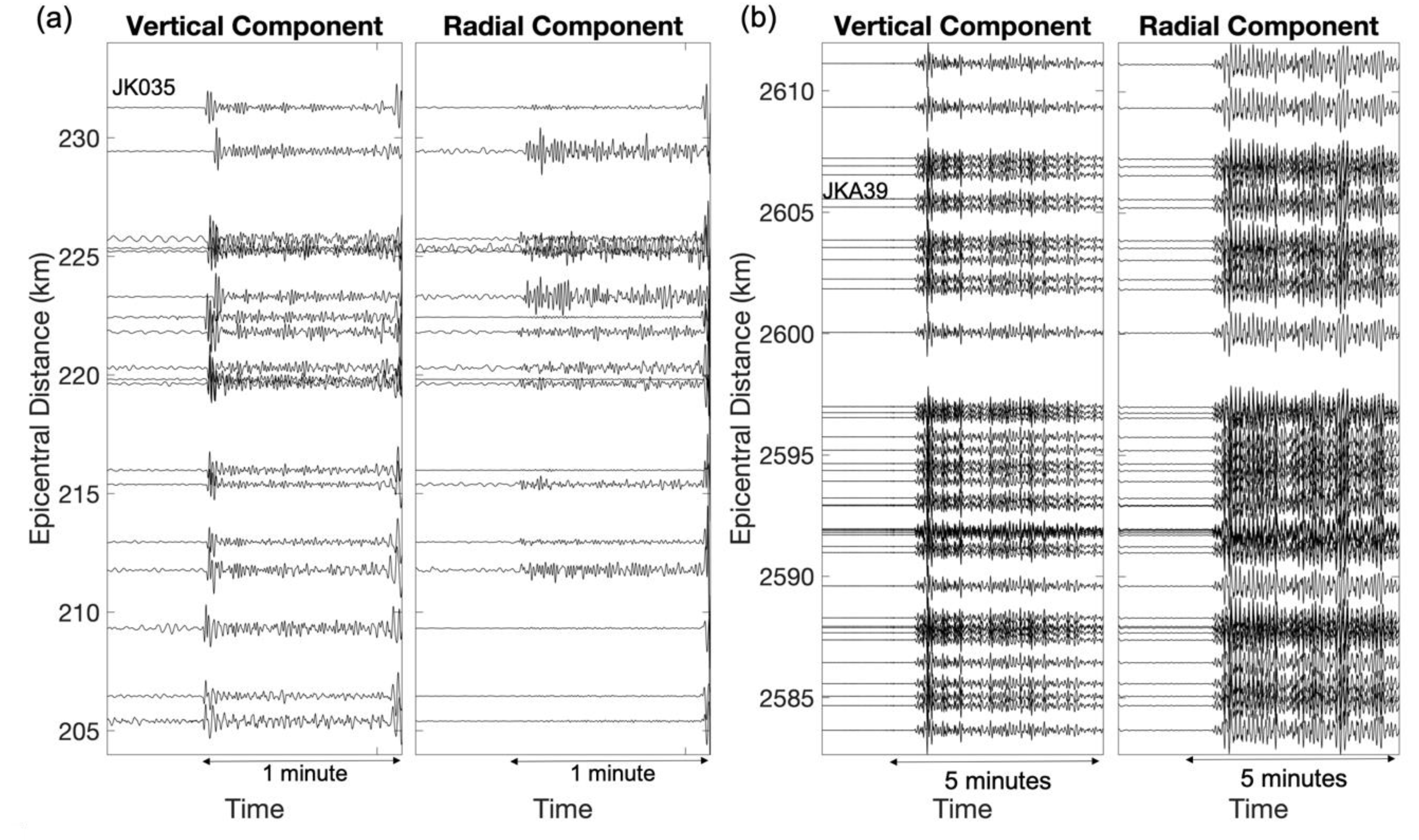
Figure 2 shows examples of a regional and a teleseismic earthquake recorded at one of the stations. The band-pass filters of 0.1–2 Hz and of 0.1–1 Hz are used for the regional earthquake and the teleseismic earthquake, respectively. Their P-waves can be clearly distinguished. Obviously, the duration of the teleseismic earthquake is much longer. Then, the calculation of their polarizations using PCA is illustrated by Figure 3 and Figure 4. The onsets are used as the starting point of the time window.
The length of the time window that can be exploited in selecting the signals may vary from very short to significantly long, and they affect the estimation. Depending on the time window length, the result of polarization direction can vary significantly, as shown in Figure 3b and Figure 4b. These differences may result in bias and/or high uncertainty in the estimation of seismic velocities. Choosing a stable and consistent polarization becomes crucial at this point.
A shorter window achieves a purely direct P-wave signal that is uncontaminated by phases of different wave type or incidence angle, but is not necessarily stable owing to its small number of data points. A longer window may contain phases of different wave type or incidence angle, which could bias the result. The synthetic tests (Appendix A) shows that window lengths greater than 1–2 seconds are unreliable due to the contamination of converted waves from the basin basement. Therefore, we analyzed each record to judge whether a mean estimate of P-wave incidence angle could be made, while removing outliers at the beginning and end of the window that might represent instability due to limited data or contamination by converted phases, respectively.
4.2. Apparent Half-Space Velocity Estimates
A station may observe several earthquakes during its recording duration, each of which contributes measurements of P-wave polarizations. These body-wave polarizations are then used to estimate apparent half-space velocities (Vsahs) beneath the station. A grid-search optimization was undertaken using Equation (7) for every station, while ray parameters were calculated from the AK135 1-D earth model [26]. Figure 5 shows plots of the apparent incidence angles as a function of ray parameter for station JKA12. Stations that record only a few earthquakes will have poorly constrained apparent half-space velocities, so we only utilized stations that recorded at least four clear earthquakes. Aiming to get the best fit model, Vsahs were searched from 50 m/s to 2000 and 4000 m/s using increments of 10 m/s.
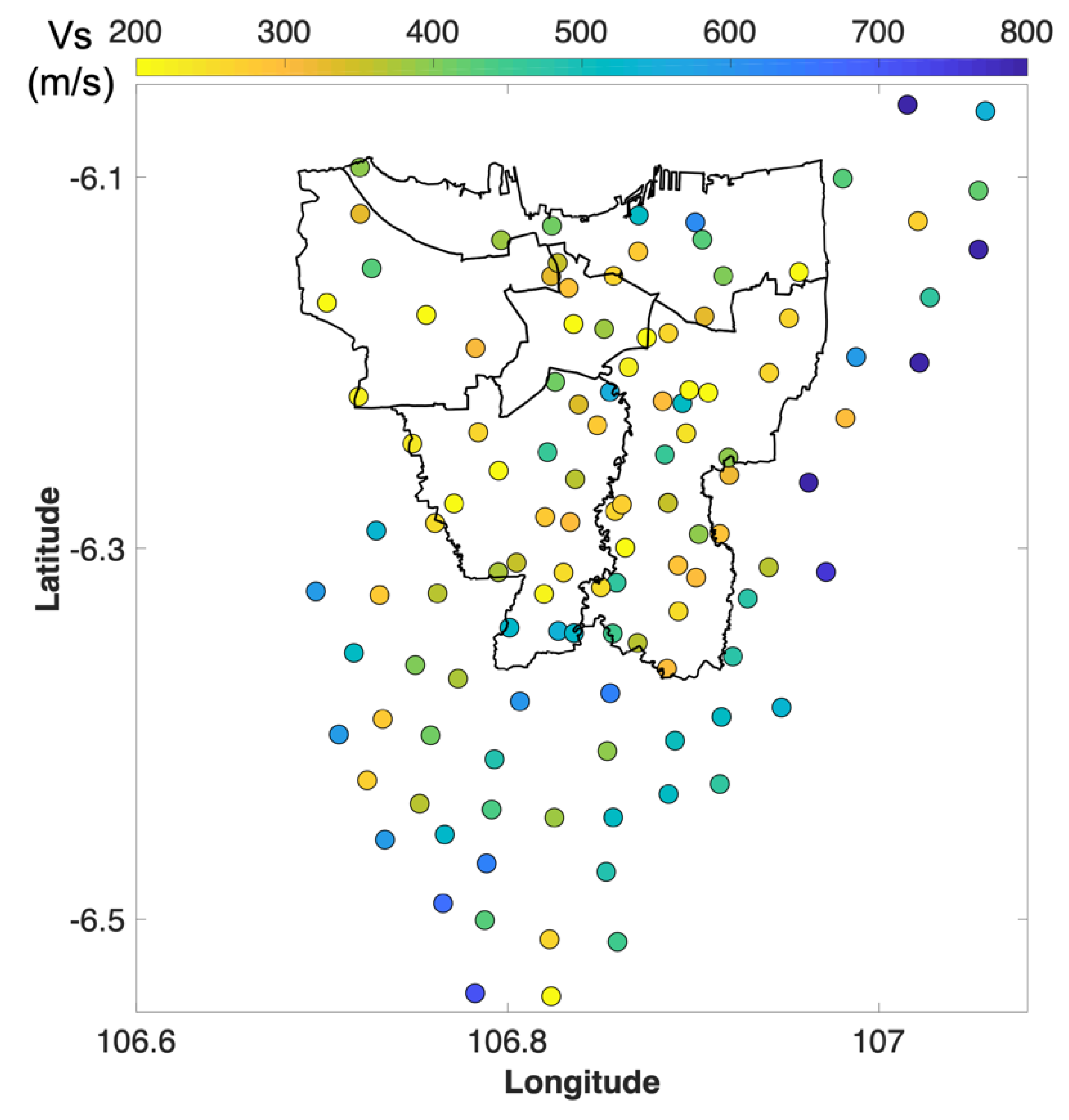
The maps of apparent half-space velocities Vsahs within Jakarta and its vicinity are shown in Figure 6. Note that stations that lack data were not included in the results. We focus on the Vsahs results derived mainly from the relatively high-quality P-wave polarization measurements.
The estimated values of Vsahs range from 200 to 800 m/s. Within the boundary of Jakarta, most of the area is dominated by low Vsahs between 200 and 400 m/s. The area characterized by low Vsahs extends outward beyond the city, only to the southwest. On the other hand, the eastern edge of the city is characterized by higher Vsahs, especially outside the city’s eastern boundary. Unexpectedly, given the results of previous studies, higher Vsahs can also be observed in the northern part of the city very near to the coastline.
4.3. Comparison and Depth Estimation
The polarization technique appears to provide considerable information on the variation in the shallow structure within the Jakarta basin, as reflected in the measured Vsahs. Unfortunately, it is difficult to know what depth range these apparent half-space values correspond to. In their use of a similar technique for measuring apparent half-space Vs from receiver functions, it is noted by Svenningsen and Jacobsen [22] that the results depend on the frequency content of the signals used. They advocate narrow-band filtering centered on inverse period f = 1/T to estimate a curve Vsahs(T) that can be inverted for the shear-wave velocity profile. Given the complications that the basin structure may pose for receiver function computation, as well as the use of local and teleseismic events with varying frequency content, we adopted the simpler approach of Park and Ishii [12]. Comparison of their estimates for Vpahs and Vsahs at stations of Japan’s broadband network Hi-net, allowed Park and Ishii [12] to conclude that their results were representative of the top ~100 m of the Vp and Vs profiles, respectively.
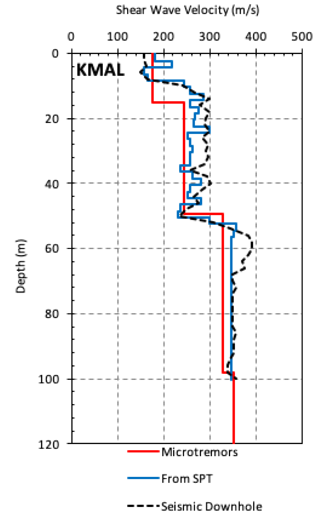
Therefore, in order to assess whether our half-space velocity measurements are representative of shallow Vs structure and if so, to suggest a depth range to which they correspond, we compared our results to previous studies. Ridwan et al. [14] used the spatial autocorrelation (SPAC) method to estimate depth profiles of Vs for depths less than 1 km at 55 sites throughout Jakarta. They provide a good set of benchmark Vs profiles at their site KMAL, located in northwest Jakarta, where they compared their SPAC result with cone penetrometer (SPT) and downhole seismic measurements (Figure 7, modified from Figure 10c in Ridwan et al. [14]). From Ridwan et al. [14], the shear-wave velocity at a depth of 100 m beneath the site KMAL is 350 m/s. Our closest station to this site, which is 700 m away, is JK046, where we used the polarization technique to obtain a very similar estimate for Vsahs of 390 m/s. The small difference between these values could reflect either measurement error or be a genuine difference in Vs due to the slight difference in the locations of measurement.
As discussed above, Cipta et al. [16] applied HVSR analysis to the 2013–2104 deployment data to obtain the Vs structure beneath Jakarta. We compared our results with average values of Cipta et al.’s [16] Vs profiles taken over different depths from the surface. We found that our results best match Cipta et al.’s [16] Vs profiles when the latter are averaged over the top 150 m, as shown in Figure 8. Note that the different samples shown are due to the lack of observed earthquakes at some stations in our study.
By comparison to the benchmark site KMAL [14], our Vsahs matches the average of the Vs profile over the top 100 m reasonably well. Unfortunately, no data deeper than that is available and one site is insufficient to indicate an overall trend. Meanwhile, our Vsahs estimates agree with many of the 150 m depth values of the much wider dataset of average Vs profiles obtained in [16]. A few inconsistencies do exist, but these may be due to anomalies in the measurements such as misalignment or miscalibration of sensors. In any case, our comparisons with previous studies suggests that the Vsahs estimates obtained in this study approximately represent average Vs at around the top 150 m depth.
4.4. Correlation with Surface Geology
The distribution of low Vsahs agrees with the geologic mapping that shows sedimentary deposits comprise almost all areas of Jakarta’s surface geology. Although the contrast between Holocene and Pleistocene deposits is small and their boundary is not well resolved in our Vsahs map, their deposits obviously fill the Jakarta basin to a depth of at least 150 m. These deposits reach the outer part of the Jakarta administrative margin mostly to the southwest, more than 10 km away. The result is in accordance with Cipta et al. [20] who reported the estimation of the basin extension based on extrapolation of the basement depth.
The higher Vsahs found in the southern part of the basin may relate to Tertiary volcanic deposits, or even the edges of the basin, which is Tertiary rock. This feature gets more distinct in the eastern part of Jakarta. The gradation from low Vsahs to higher Vsahs at the eastern administrative boundary underlines the contrast between sedimentary deposits and denser rock. The sedimentary deposits diminish eastward, while the thinnest layer lies at the southeastern corner of our study area. We suggest that the basin edge emerges near the surface in this area.
5. Conclusions
We applied the simple body-wave polarization technique of Park and Ishii [12] to obtain the variation in apparent half-space S-wave velocity (Vsahs) over the Jakarta Basin. By measuring the apparent incidence angles of earthquake-generated P-waves using principal component analysis, we obtained estimates of Vsahs. Although care had to be taken in choosing window lengths to avoid contamination of the direct P-wave by basement converted phases, we found we were able to obtain stable estimates of polarization by choosing windows of 1–2 sec duration.
The spatial variations we observed in Vsahs estimated using the body-wave polarization technique seem sensible when compared to other studies. In particular, when comparing our Vsahs with the Vs profiles in [14] and [16], the mapping of Vsahs appears to be correlated to the average of Vs profiles over the top 150 meters. In further studies, it might be useful to investigate the frequency-dependence of body-wave polarization in an attempt to reveal further details of the shallow Vs profiles.
Our estimates of Vsahs reflect the shallow Vs structure obtained within the Jakarta city limits in earlier studies [15,16], but extended this information beyond the city limits of Jakarta to what is thought to be the basin edge [20]. Although the surface geology of the entire study area is composed of quaternary sediments (Figure 1b), we found that on average, Vsahs increases towards the outer edge of the study area (Figure 6). This may indicate that Vsahs is sensitive to a reduction in basement depth that indicates the effective edge of the basement. In future studies we hope to obtain a more complete geometry of the Jakarta sedimentary basin that will enable a more accurate ground-motion simulation for hypothetical earthquake scenarios that can characterize seismic risk in Jakarta.
Author Contributions
R.V.R., P.C., S.W. conceived the study and contributed to the writing of the manuscript. All authors contributed to the preparation of the manuscript. The data and material that support the findings of this study are available on request from the corresponding author, R.V.R.
Funding
This study was partly supported through the ITB Research Grant 2018 awarded to SW and RVR and partly supported through the ANU Research Grant 2018 awarded to PC.
Acknowledgments
We gratefully acknowledge the Institute of Technology Bandung (ITB) and the Australian National University (ANU) for funding this research. We also thank the Australia Awards for the scholarship awarded to RVR and conducting this research at RSES, ANU.
Conflicts of Interest
We declare that we have no significant competing financial, professional or personal interests that might have influenced the performance or presentation of the work described in this manuscript. The funders had no role in the design of the study; in the collection, analyses, or interpretation of data; in the writing of the manuscript, or in the decision to publish the results.
Appendix A. Synthetic Test
As mentioned above, the idea of estimating the P-waves polarization relies greatly on the windowing to isolate P-wave signals, with window length chosen to include as much of the direct P waveform as possible without including coda that is contaminated by arrivals of different wave type or incidence angle. A complication arises in sedimentary basins due to the possible contamination from arrivals of phases converted at the basement which will arrive with a different incidence angle.

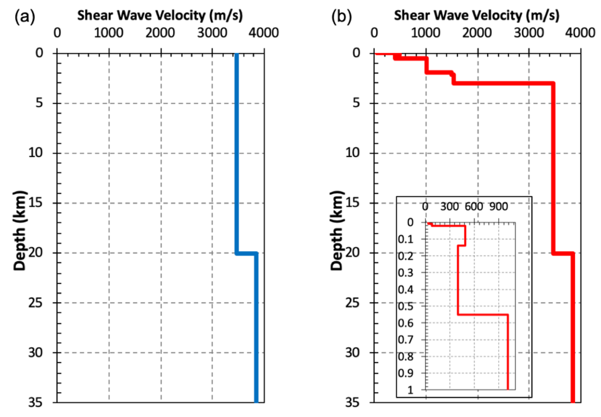
We performed synthetic tests to examine the effect of the converted wave in the Jakarta Basin. We generated a seismogram for the incoming P-wave based on a layered half-space model [27] for the Bohol, Philippines Mw 7.2 earthquake, which occurred on 2013 October 15. The ray parameter of the direct P-waves is 9.14 s/deg−1. Seismograms for two different velocity models were generated, one for the AK135 1-D earth model [26] (Figure A1a) and the second for the AK135 model with the insertion of layers in the top 3 km representing the sedimentary fill of the Jakarta Basin [16] (Figure A1a).
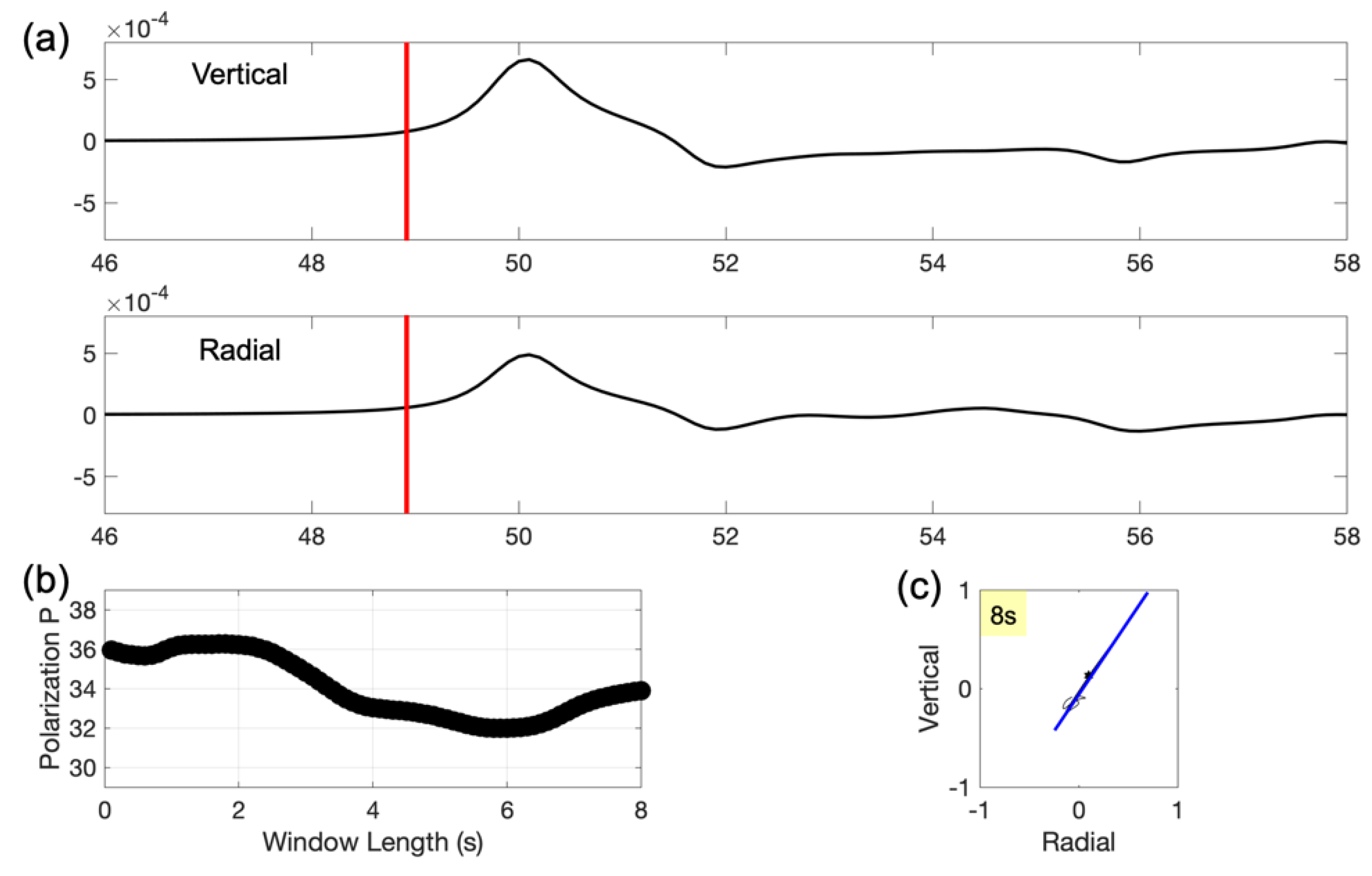
As shown in Figure A2, the waveforms of the direct P-wave on vertical and radial components correlate very well. There are no obvious differences in the vertical- vs. radial-component waveforms that might indicate the presence of converted waves. Using window lengths varying from 1 to 8 seconds, the calculated P-wave incidence angle varied between 32 and 36 degrees. Applying Equation (2), the calculated Vsahs are 3.35 km/s and 3.75 km/s, respectively. These values seem reasonably consistent with the Vs = 3.46 km/s in the top layer of the AK135 model.
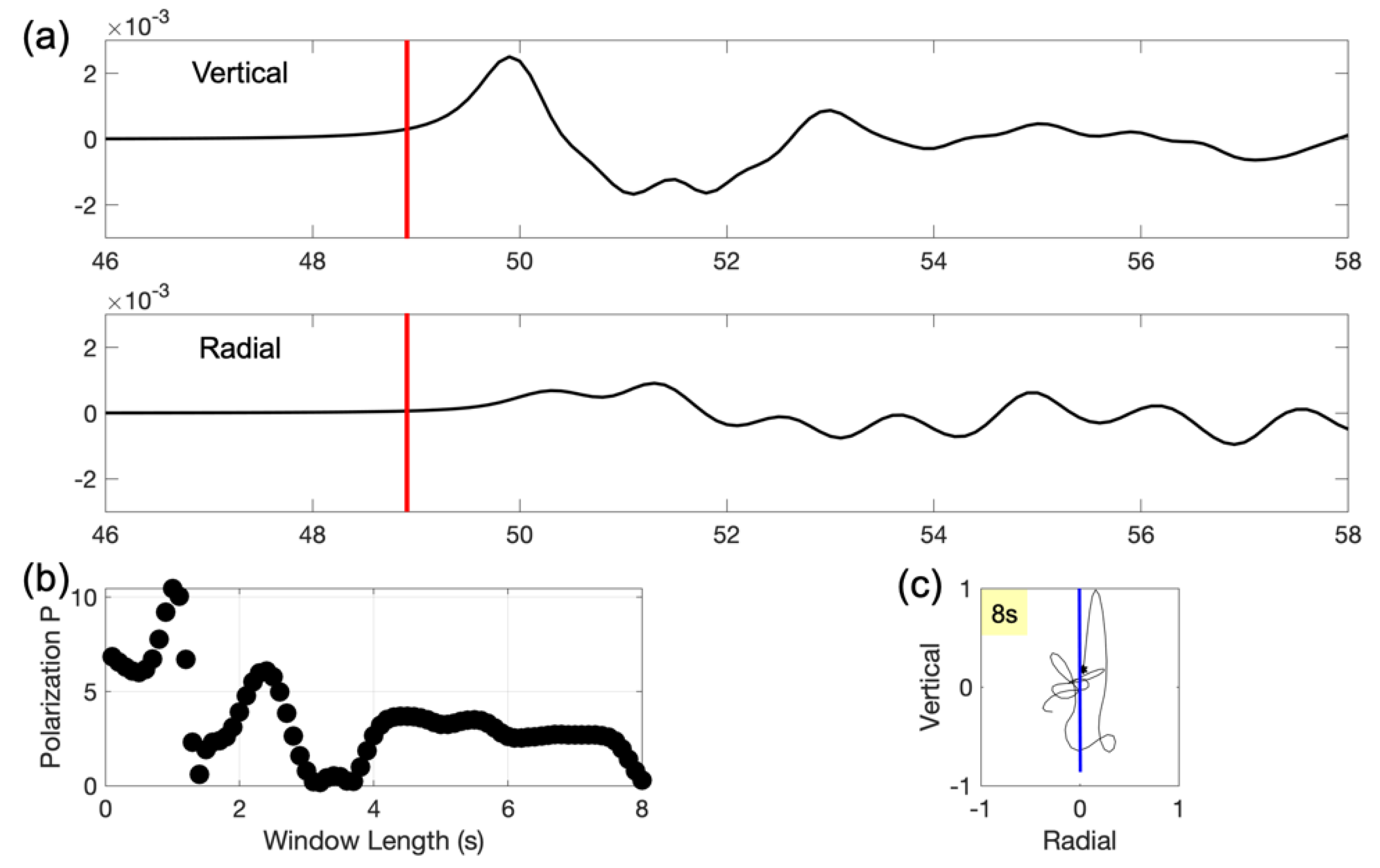
As shown in Figure A3, on the other hand, there is poor correlation between the radial and vertical components following the arrival of the direct P-wave. After 1–2 seconds following the arrival of the direct P-wave, a different phase arrives which we interpret as the arrival Ps wave converted at the basement, although it is difficult to identify clearly because of the basin’s complex velocity structure. Due to the appearance of this basement-converted wave, the use of more than 1–2 seconds for the length of window is questionable. Using time window lengths of 1 to 8 seconds resulted in a variation of measured angle of incidence between 0.1 and 10 degrees. The average Vs of the basin model in the top 100 m is 300 m/s. Applying Equation (3), then the expected polarization should be 2.6 degree. While this lies within the range of incidence angles for windows shorter than 2 seconds, it is difficult to pick the optimal window length with certainty.
Figure A2.
Seismograms of P-wave arrival in Jakarta for the Mw 7.2 Bohol earthquake at 2600 km distance, calculated for a velocity model with no sedimentary basin layers. (a) Waveforms of vertical and radial components. Red lines indicate the P-onset. (b) The variation in P-wave apparent incidence angle calculated for different time window lengths, in increments of 0.1 s, starting from the P-onset. (c) The particle motion during the 8 s window. The blue line highlights its principal component.

Figure A3.
Seismograms of P-wave arrival in Jakarta for the Mw 7.2 Bohol earthquake at 2600 km distance, calculated for a velocity model that includes sedimentary basin layers. (a) Waveforms of vertical and radial components. Red lines are P-onset. (b) Variation in P-wave apparent incidence angle calculated for different time window lengths, in increments of 0.1 s, starting from P-onset. (c) The particle motion during the 8 s window. The blue line highlights its principal component.

References
- Bilham, R. The seismic future of cities. Bull. Earthq. Eng. 2009, 7, 839–887. [Google Scholar] [CrossRef] [Green Version]
- Galetzka, J.; Melgar, D.; Genrich, J.F.; Geng, J.; Owen, S.; Lindsey, E.O.; Xu, X.; Bock, Y.; Avouac, J.-P.; Adhikari, L.B.; et al. Slip pulse and resonance of the Kathmandu basin during the 2015 Gorkha earthquake, Nepal. Science 2015, 349, 1091–1095. [Google Scholar] [CrossRef] [Green Version]
- Sahakian, V.J.; Melgar, D.; Quintanar, L.; Ramírez-Guzmán, L.; Pérez-Campos, X.; Baltay, A. Ground Motions from the 7 and 19 September 2017 Tehuantepec and Puebla-Morelos, Mexico, Earthquakes. Bull. Seismol. Soc. Am. 2018, 108, 3300–3312. [Google Scholar] [CrossRef]
- Nakamura, Y. A method for dynamic characteristics estimation of subsurface using microtremor on the ground surface. Railw. Tech. Res. Inst. Q. Rep. 1989, 30, 25–33. [Google Scholar]
- Behrou, R.; Haghpanah, F.; Foroughi, H. Empirical seismic site effect analysis for the city of Tehran using H/V and methods. Int. J. Geotech. Eng. 2018, 6362, 1–9. [Google Scholar] [CrossRef]
- Fäh, D.; Kind, F.; Giardini, D. A theoretical investigation of average H/V ratios. Geophys. J. Int. 2001, 145, 535–549. [Google Scholar] [CrossRef]
- Arai, H.; Tokimatsu, K. S-wave velocity profiling by joint inversion of microtremor dispersion curve and horizontal-to-vertical (H/V) spectrum. Bull. Seismol. Soc. Am. 2005, 95, 1766–1778. [Google Scholar] [CrossRef]
- Young, M.K.; Rawlinson, N.; Bodin, T. Transdimensional inversion of ambient seismic noise for 3D shear velocity structure of the Tasmanian crust. Geophysics 2013, 78, WB49–WB62. [Google Scholar] [CrossRef] [Green Version]
- Shapiro, N.; Campillo, M. Emergence of broadband Rayleigh waves from correlations of the ambient seismic noise. Geophys. Res. Lett. 2004, 31, 8–11. [Google Scholar] [CrossRef]
- Denolle, M.A.; Miyake, H.; Nakagawa, S.; Hirata, N.; Beroza, G.C. Long-period seismic amplification in the Kanto Basin from the ambient seismic field. Geophys. Res. Lett. 2014, 41, 2319–2325. [Google Scholar] [CrossRef]
- Zheng, D.; Saygin, E.; Cummins, P.; Ge, Z.; Min, Z.; Cipta, A.; Yang, R. Transdimensional Bayesian seismic ambient noise tomography across SE Tibet. J. Asian Earth Sci. 2017, 134, 86–93. [Google Scholar] [CrossRef]
- Park, S.; Ishii, M. Near-surface compressional and shear wave speeds constrained by body-wave polarization analysis. Geophys. J. Int. 2018, 213, 1559–1571. [Google Scholar] [CrossRef]
- Lubis, R.F.; Sakura, Y.; Delinom, R. Groundwater recharge and discharge processes in the Jakarta groundwater basin, Indonesia. Hydrogeol. J. 2008, 16, 927–938. [Google Scholar] [CrossRef]
- Ridwan, M.; Widiyantoro, S.; Irsyam, M.; Yamanaka, H. Development of an engineering bedrock map beneath Jakarta based on microtremor array measurements. Geol. Soc. London Spec. Publ. 2016, 441, 153–165. [Google Scholar] [CrossRef]
- Saygin, E.; Cummins, P.R.; Cipta, A.; Hawkins, R.; Pandhu, R.; Murjaya, J.; Masturyono, J.; Irsyam, M.; Widiyantoro, S.; Kennett, B.L.N. Imaging architecture of the Jakarta Basin, Indonesia with transdimensional inversion of seismic noise. Geophys. J. Int. 2016, 204, 918–931. [Google Scholar] [CrossRef]
- Cipta, A.; Cummins, P.; Dettmer, J.; Saygin, E.; Irsyam, M.; Rudyanto, A.; Murjaya, J. Seismic velocity structure of the Jakarta Basin, Indonesia, using trans-dimensional Bayesian inversion of horizontal-to-vertical spectral ratios. Geophys. J. Int. 2018, 215, 431–449. [Google Scholar] [CrossRef] [Green Version]
- Turkandi, T.; Sidarto, A.D.; Purbohadiwidjojo, M. Geologic Map of the Jakarta and Kepulauan Seribu Quadrangle Java; Geological Agency: Bandung, Indonesia, 1992. [Google Scholar]
- Van-Bemmelen, R. The Geology of Indonesia, Vol 1A, General Geology of Indonesia and Adjacent Archipelagoes; Government Printing House: Hague, The Netherlands, 1949.
- Anderson, J.G.; Bodin, P.; Brune, J.N.; Prince, J.; Singh, S.K.; Quaas, R.; Onate, M. Strong ground motion from the Michoacan, Mexico, earthquake. Science 1986, 233, 1043–1049. [Google Scholar] [CrossRef]
- Cipta, A.; Cummins, P.; Irsyam, M.; Hidayati, S. Basin Resonance and Seismic Hazard in Jakarta, Indonesia. Geosciences 2018, 8, 128. [Google Scholar] [CrossRef]
- Wiechert, E. Über Erdbebenwellen. Part I: Theoretisches über die. Ausbreitung der Erdbebenwellen, Nachrichten von der Königlichen. Gesellschaft der Wissenschaften zu Göttingen. Math. Klasse 1907, 415–549. [Google Scholar]
- Svenningsen, L.; Jacobsen, B.H. AbsoluteS-velocity estimation from receiver functions. Geophys. J. Int. 2007, 170, 1089–1094. [Google Scholar] [CrossRef]
- Jolliffe, I.T. Principal Component Analysis, 2nd ed.; Springer: New York, NY, USA, 2002; Volume 98, ISBN 0-387-95442-2. [Google Scholar]
- Knapmeyer, M. TTBox: A MatLab Toolbox for the Computation of 1D Teleseismic Travel Times. Seism. Res. Lett. 2004, 75, 726–733. [Google Scholar] [CrossRef]
- Baillard, C.; Crawford, W.C.; Ballu, V.; Hibert, C.; Mangeney, A. An automatic kurtosis-based P-and S-phase picker designed for local seismic networks. Bull. Seismol. Soc. Am. 2013, 104, 394–409. [Google Scholar] [CrossRef]
- Kennett, B.L.N.; Engdahl, E.R.; Buland, R. Constraints on seismic velocities in the Earth from traveltimes. Geophys. J. Int. 1995, 122, 108–124. [Google Scholar] [CrossRef]
- Wang, R. A simple orthonormalization method for stable and efficient computation of Green’s functions. Bull. Seismol. Soc. Am. 1999, 89, 733–741. [Google Scholar]
Figure 1.
(a) Distribution of earthquakes (yellow circles) observed around the study area (red zone). (b) Map of the seismic deployments and surface geology around Jakarta (modified from [20]). The inverted triangles represent the seismic network deployed between October 2013 and February 2014. The squares represent the seismic network deployed between April 2018 and October 2018. The administrative boundary of Jakarta is shown with black lines. The blue cross is the benchmark site KMAL. The colors represent the number of events observed at each station, while the colorless stations did not record any useful earthquake signals.

Figure 2.
Examples of recorded earthquakes signals at stations shown in vertical and radial components. (a) Regional Mw 5.3 earthquake which occurred on 22 June 2018 in the Java Sea; (b) Teleseismic Mw 7.2 earthquake which occurred on 15 October 2013 in Bohol, the Philippines.
Figure 2.
Examples of recorded earthquakes signals at stations shown in vertical and radial components. (a) Regional Mw 5.3 earthquake which occurred on 22 June 2018 in the Java Sea; (b) Teleseismic Mw 7.2 earthquake which occurred on 15 October 2013 in Bohol, the Philippines.

Figure 3.
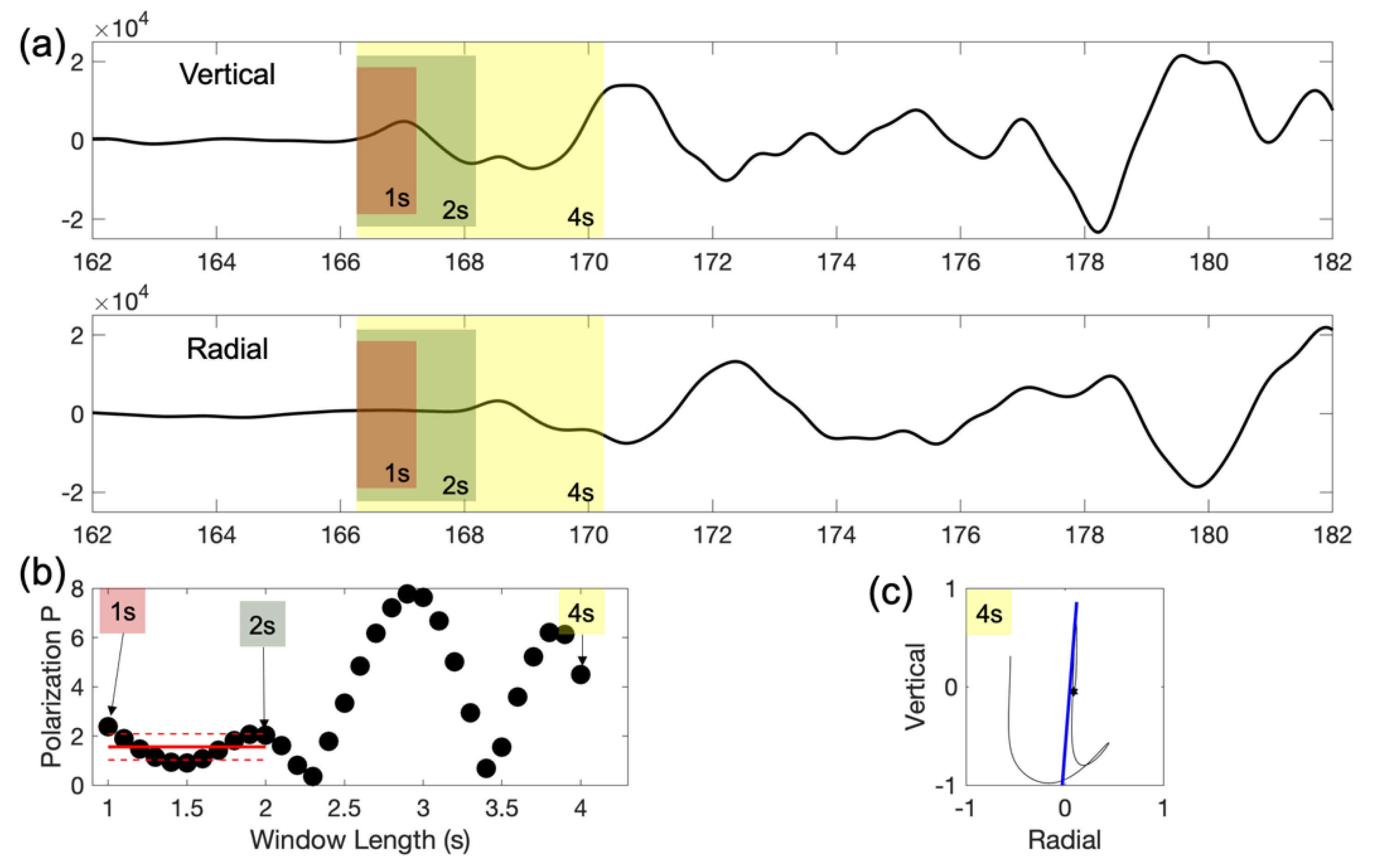
Polarization analysis of P-waves at station JK035 for the Mw 5.3 regional earthquake. The azimuth is 230° and the epicentral distance is 231 km. (a) Time windowing used for principal component analysis (PCA), with window lengths of 1, 2, and 4 seconds indicated by red, green, and yellow shades, respectively. (b) Distribution of P-wave polarizations calculated from different lengths of the time window, in increments of 0.1 s. The red line represents the best polarization after removing outliers. (c) The particle motion during the 4-s window. The blue line highlights its principal component.
Figure 3.
Polarization analysis of P-waves at station JK035 for the Mw 5.3 regional earthquake. The azimuth is 230° and the epicentral distance is 231 km. (a) Time windowing used for principal component analysis (PCA), with window lengths of 1, 2, and 4 seconds indicated by red, green, and yellow shades, respectively. (b) Distribution of P-wave polarizations calculated from different lengths of the time window, in increments of 0.1 s. The red line represents the best polarization after removing outliers. (c) The particle motion during the 4-s window. The blue line highlights its principal component.

Figure 4.
Polarization analysis of P-wave at station JKA39 for the Mw 7.2 teleseismic earthquake. The azimuth is 227° and the epicentral distance is 2605 km. (a) Time windowing used for PCA, with window lengths of 1, 2, and 4 seconds, indicated by red, green, and yellow shades, respectively. (b) Distribution of P-wave polarizations calculated from different lengths of the time window, in increments of 0.1 s. The red line represents the best polarization after removing outliers. (c) The particle motion during the 4 s. The blue line highlights its principal component.

Figure 5.
Observed (a) P-wave incidence angles (colored circles) at station JKA39, as a function of theoretical ray parameters computed using the AK135 model. The colors represent the weighting values. Black lines represent the best fitting calculated angles. (b) Grid-search results for station JKA39 along its misfit, with the best fit marked by the red star. (c) and (d) Same as (a) and (b), respectively, but at station JK035.

Figure 6.
Map of near-surface shear-wave velocities represented by colored circles. Yellow is low and blue is high, ranging from 200 to 800 m/s.
Figure 6.
Map of near-surface shear-wave velocities represented by colored circles. Yellow is low and blue is high, ranging from 200 to 800 m/s.

Figure 7.
Vs profiles at the site KMAL obtained from microtremor arrays (red line), standard penetration testing (SPT) (blue line) and seismic downhole (dashed line). Modified from [14].
Figure 7.
Vs profiles at the site KMAL obtained from microtremor arrays (red line), standard penetration testing (SPT) (blue line) and seismic downhole (dashed line). Modified from [14].

Figure 8.
Map of near-surface shear-wave velocities represented by colored circles. Yellow is low and blue is high, ranging from 200 to 800 m/s. (a) Vsahs obtained in this study based on body-wave polarization. (b) Average Vs over depths in the top 150 m obtained from the HVSR study [16]. (c) The scatter plot between the Vsahs estimates and the HVSR study; black solid line is the linear regression line and the grey dashed line is the 1:1 line. (d) Absolute difference between (a) and (b).

© 2019 by the authors. Licensee MDPI, Basel, Switzerland. This article is an open access article distributed under the terms and conditions of the Creative Commons Attribution (CC BY) license (http://creativecommons.org/licenses/by/4.0/).
Share and Cite
MDPI and ACS Style
Ry, R.V.; Cummins, P.; Widiyantoro, S. Shallow Shear-Wave Velocity Beneath Jakarta, Indonesia Revealed by Body-Wave Polarization Analysis. Geosciences 2019, 9, 386. https://0-doi-org.brum.beds.ac.uk/10.3390/geosciences9090386
AMA Style
Ry RV, Cummins P, Widiyantoro S. Shallow Shear-Wave Velocity Beneath Jakarta, Indonesia Revealed by Body-Wave Polarization Analysis. Geosciences. 2019; 9(9):386. https://0-doi-org.brum.beds.ac.uk/10.3390/geosciences9090386
Chicago/Turabian StyleRy, Rexha Verdhora, Phil Cummins, and Sri Widiyantoro. 2019. "Shallow Shear-Wave Velocity Beneath Jakarta, Indonesia Revealed by Body-Wave Polarization Analysis" Geosciences 9, no. 9: 386. https://0-doi-org.brum.beds.ac.uk/10.3390/geosciences9090386
Note that from the first issue of 2016, this journal uses article numbers instead of page numbers. See further details here.