
Critical Assessment of Land Use Land Cover Dynamics Using Multi-Temporal Satellite Images


Abstract
:1. Introduction
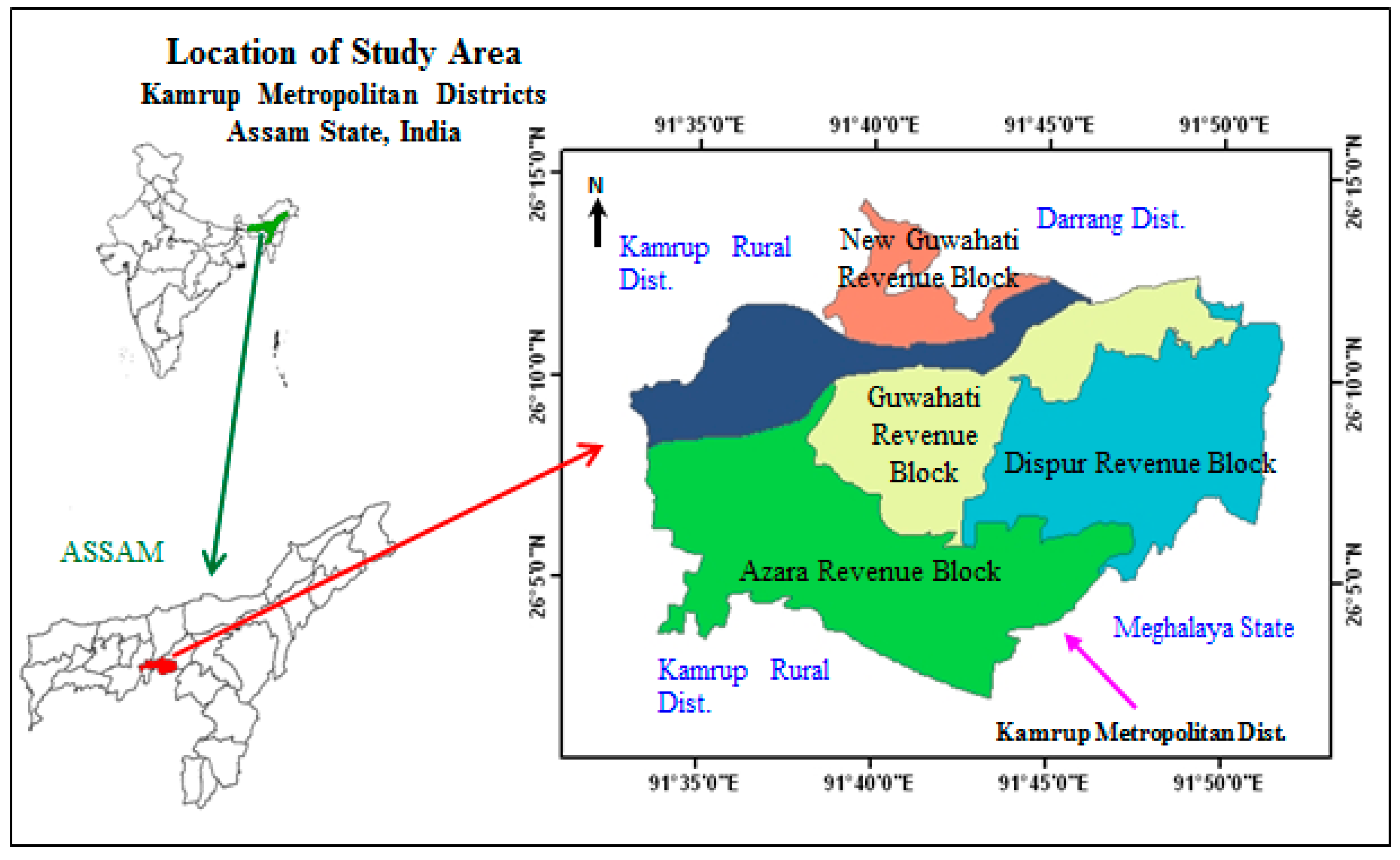
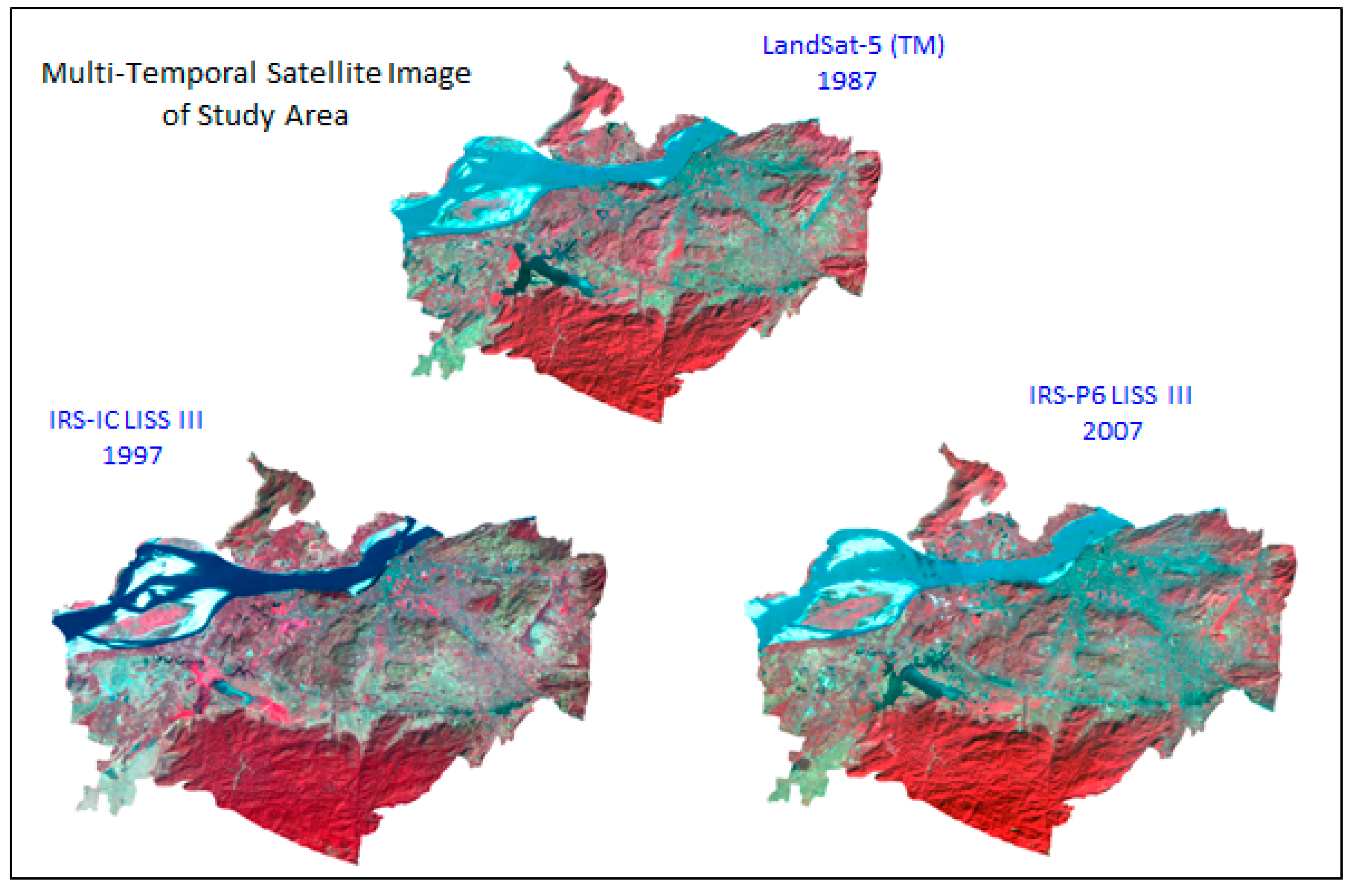
2. Study Area and Data Used


| Satellite | Sensor | Path/Row | Data Acquired | Spatial Resolution (Meters) | Spectral Band | Data Sources |
|---|---|---|---|---|---|---|
| LANDSAT-5 | TM | 136/042 (WRS-2 footprints) | 26-12-1987 | 30 (120 m–thermal (B 6)) | B 1 (blue): 0.45–0.52 µm | GLCF *-Earth Science Data Interface |
| B 2 (green): 0.52–0.60 µm | ||||||
| B 3 (red): 0.63–0.69 µm | ||||||
| B 4 (NIR): 0.76–0.90 µm | ||||||
| B 5 (SWIR): 1.55–1.75 µm | ||||||
| B 6 (thermal IR):10.4–12.5 µm | ||||||
| B 7 (Mid–Infrared): 2.08–2.35 µm | ||||||
| IRS-1C | LISS-III | 110/53 | 05-03-1997 | 23.5 (70 m–B5 (SWIR) ) | B 2 (green): 0.52–0.59 µm | NRSC |
| B 3 (red): 0.62–0.68 µm | ||||||
| B 4 (NIR): 0.77–0.86 µm | ||||||
| B 5 (SWIR): 1.55–1.70 µm | ||||||
| IRS-P6 (Resourcesat-1) | LISS-III | 110/53 | 14-12-2007 | 23.5 | B 2 (green): 0.52–0.59 µm | NRSC |
| B 3 (red): 0.62–0.68 µm | ||||||
| B 4 (NIR): 0.77–0.86 µm | ||||||
| B 5 (SWIR): 1.55–1.70 µm |

| Data | Data Sources | Scale |
|---|---|---|
| Topographic Sheet No. 72N/12 and 72N/16 | Survey of India (SOI) | 1:50,000 |
| Master Plan of Guwahati | Guwahati Metropolitan Development Authority (GMDA) | 1:25,000 |
| Maps | Guwahati Metropolitan Development Authority (GMDA) | |
| Guwahati Municipal Corporation (GMC) | ||
| Kamrup Metropolitan District—National Informatics Centre (NIC) | - | |
| IKONOS, QUICKBIRD Satellite Images | www.earth.google.com |
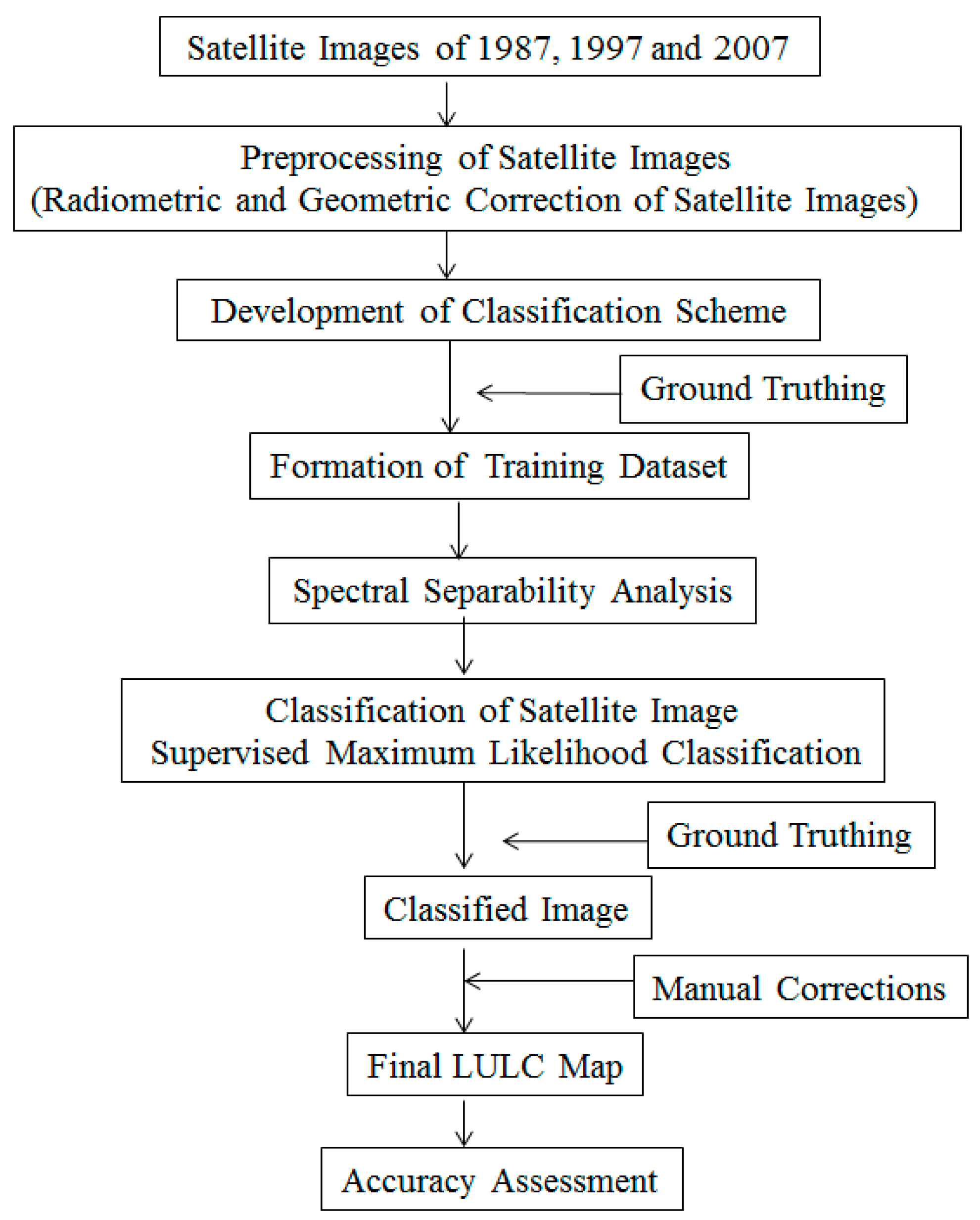
3. Methodology
3.1. Preparation of Land Use Land Cover (LULC) Map

3.2. Quantity of Land Use Land Cover Change (LULUC)
| Level I | Level II |
|---|---|
| 1. Built up Land | 1.1. Built up Land |
| 2. Agricultural Land | 2.1. Agricultural Crop Land |
| 2.2. Agricultural Fallow Land | |
| 2.3. Plantations | |
| 3.Forest | 3.1. Dense Forest |
| 3.2. Degraded Forest | |
| 4.Waste Land | 4.1. Land with or without Scrub |
| 4.2. Marshy/Swampy | |
| 4.3. Waterlogged Area | |
| 4.4. Sandy Area (River Bed) | |
| 5. Water Bodies | 5.1. River/Stream |
| 5.2. Lake/Reservoir/Pond/Tank | |
| 6. Others | 6.1. Open Land |
| 6.2. Aquatic Vegetation |
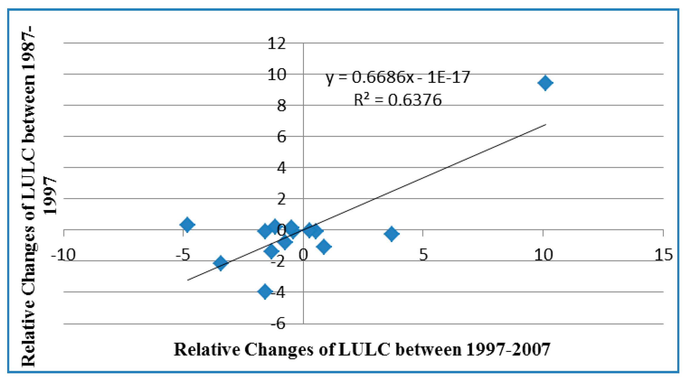
3.2.1. Relative Changes of LULC
3.2.2. Gross Gains, Gross Losses and Persistence of LULC
3.2.3. Net Change and Swap Change of LULC
3.3. Allocation of Land Use Land Cover Change (LULUC)
4. Results and Discussions
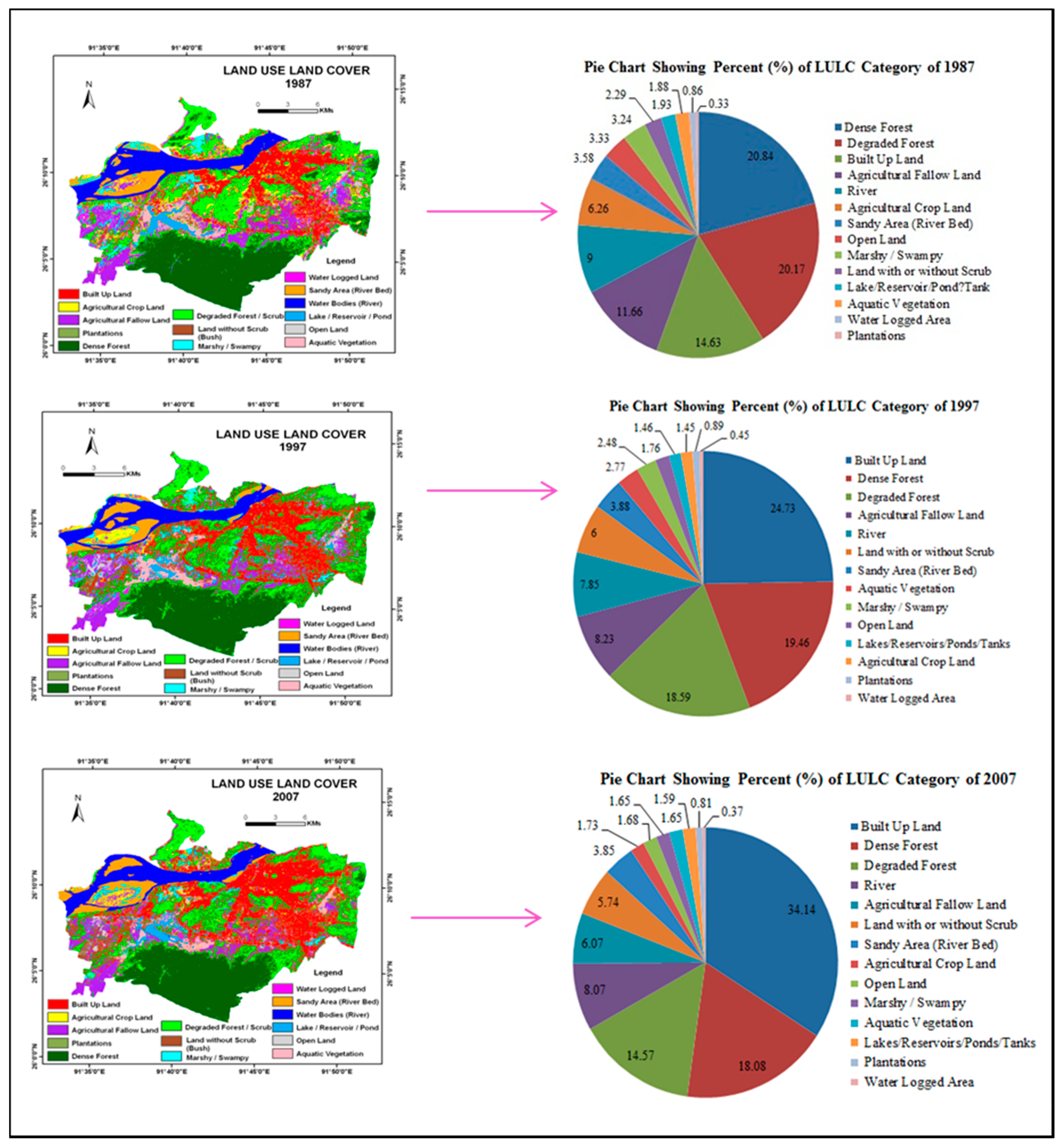
4.1. Results of Land Use Land Cover Classification
| Sl. No. | Class Name | 1987 | 1997 | 2007 | |||
|---|---|---|---|---|---|---|---|
| Area (Km²) | % of Area | Area (Km²) | % of Area | Area (Km²) | % of Area | ||
| 1. | Built up Land | 60.54 | 14.63 | 102.4 | 24.73 | 141.35 | 34.14 |
| 2. | Agricultural Crop Land | 25.91 | 6.26 | 5.99 | 1.45 | 7.17 | 1.73 |
| 3. | Agricultural Fallow Land | 48.27 | 11.66 | 34.08 | 8.23 | 25.12 | 6.07 |
| 4. | Plantations | 1.38 | 0.33 | 3.68 | 0.89 | 3.35 | 0.81 |
| 5. | Dense Forest | 86.26 | 20.84 | 80.56 | 19.46 | 74.84 | 18.08 |
| 6. | Degraded Forest | 83.48 | 20.17 | 76.95 | 18.59 | 60.31 | 14.57 |
| 7. | Land with or without Scrub | 9.48 | 2.29 | 24.82 | 6 | 23.78 | 5.74 |
| 8. | Marshy/Swampy | 13.42 | 3.24 | 10.26 | 2.48 | 6.82 | 1.65 |
| 9. | Water Logged Area | 3.57 | 0.86 | 1.86 | 0.45 | 1.52 | 0.37 |
| 10. | Sandy Area (River Bed) | 14.83 | 3.58 | 16.08 | 3.88 | 15.92 | 3.85 |
| 11. | River/Stream | 37.27 | 9 | 32.51 | 7.85 | 33.42 | 8.07 |
| 12. | Lake/Reservoir/Pond/Tank | 7.99 | 1.93 | 6.05 | 1.46 | 6.59 | 1.59 |
| 13. | Open Land | 13.8 | 3.33 | 7.28 | 1.76 | 6.97 | 1.68 |
| 14. | Aquatic Vegetation | 7.78 | 1.88 | 11.46 | 2.77 | 6.82 | 1.65 |
| Total | 413.98 | 100.00 | 413.98 | 100.00 | 413.98 | 100.00 | |
4.1.1. Quantity of Land Use Land Cover (LULC)

4.1.2. Allocation of Land Use Land Cover (LULC)
4.2. Changes in Quantity of LULC
4.2.1. Relative Changes in Quantity of LULC
| Sl. | Class Name | 1987 | 1997 | Relative Change between 1987 and 1997 | |||
|---|---|---|---|---|---|---|---|
| Area (Km²) | % of Area | Area (Km²) | % of Area | Area in Km² | Area in % | ||
| 1. | Built up Land | 60.54 | 14.63 | 102.4 | 24.73 | 41.86 | 10.12 |
| 2. | Agricultural Crop Land | 25.91 | 6.26 | 5.99 | 1.45 | −19.92 | −4.82 |
| 3. | Agricultural Fallow Land | 48.27 | 11.66 | 34.08 | 8.23 | −14.19 | −3.42 |
| 4. | Plantations | 1.38 | 0.33 | 3.68 | 0.89 | 2.3 | 0.55 |
| 5. | Dense Forest | 86.26 | 20.84 | 80.56 | 19.46 | −5.7 | −1.33 |
| 6. | Degraded Forest | 83.48 | 20.17 | 76.95 | 18.59 | −6.53 | −1.58 |
| 7. | Land with or without Scrub | 9.48 | 2.29 | 24.82 | 6 | 15.34 | 3.7 |
| 8. | Marshy/Swampy | 13.42 | 3.24 | 10.26 | 2.48 | −3.16 | −0.76 |
| 9. | Water Logged Area | 3.57 | 0.86 | 1.86 | 0.45 | −1.71 | −0.41 |
| 10. | Sandy Area (River Bed) | 14.83 | 3.58 | 16.08 | 3.88 | 1.25 | 0.28 |
| 11. | River/Stream | 37.27 | 9 | 32.51 | 7.85 | −4.76 | −1.17 |
| 12. | Lake/Reservoir/Pond/Tank | 7.99 | 1.93 | 6.05 | 1.46 | −1.94 | −0.47 |
| 13. | Open Land | 13.8 | 3.33 | 7.28 | 1.76 | −6.52 | −1.58 |
| 14. | Aquatic Vegetation | 7.78 | 1.88 | 11.46 | 2.77 | 3.68 | 0.89 |
| Total | 413.98 | 100.00 | 413.98 | 100.00 | 0.0 | 0.0 | |
| Sl. | Class Name | 1997 | 2007 | Relative Change between 1997 and 2007 | |||
|---|---|---|---|---|---|---|---|
| Area (Km²) | % of Area | Area (Km²) | % of Area | Area in Km² | Area in % | ||
| 1. | Built up Land | 102.4 | 24.73 | 141.35 | 34.14 | 38.95 | 9.41 |
| 2. | Agricultural Crop Land | 5.99 | 1.45 | 7.17 | 1.73 | 1.18 | 0.28 |
| 3. | Agricultural Fallow Land | 34.08 | 8.23 | 25.12 | 6.07 | −8.96 | −2.16 |
| 4. | Plantations | 3.68 | 0.89 | 3.35 | 0.81 | −0.33 | −0.08 |
| 5. | Dense Forest | 80.56 | 19.46 | 74.84 | 18.08 | −5.72 | −1.38 |
| 6. | Degraded Forest | 76.95 | 18.59 | 60.31 | 14.57 | −16.64 | −3.98 |
| 7. | Land with or without Scrub | 24.82 | 6 | 23.78 | 5.74 | −1.04 | −0.27 |
| 8. | Marshy/Swampy | 10.26 | 2.48 | 6.82 | 1.65 | −3.44 | −0.82 |
| 9. | Water Logged Area | 1.86 | 0.45 | 1.52 | 0.37 | −0.34 | −0.08 |
| 10. | Sandy Area (River Bed) | 16.08 | 3.88 | 15.92 | 3.85 | −0.16 | −0.04 |
| 11. | River/Stream | 32.51 | 7.85 | 33.42 | 8.07 | 0.91 | 0.21 |
| 12. | Lake/Reservoir/Pond/Tank | 6.05 | 1.46 | 6.59 | 1.59 | 0.54 | 0.11 |
| 13. | Open Land | 7.28 | 1.76 | 6.97 | 1.68 | −0.31 | −0.09 |
| 14. | Aquatic Vegetation | 11.46 | 2.77 | 6.82 | 1.65 | −4.64 | −1.11 |
| Total | 413.98 | 100 | 413.98 | 100 | 0.0 | 0.0 | |
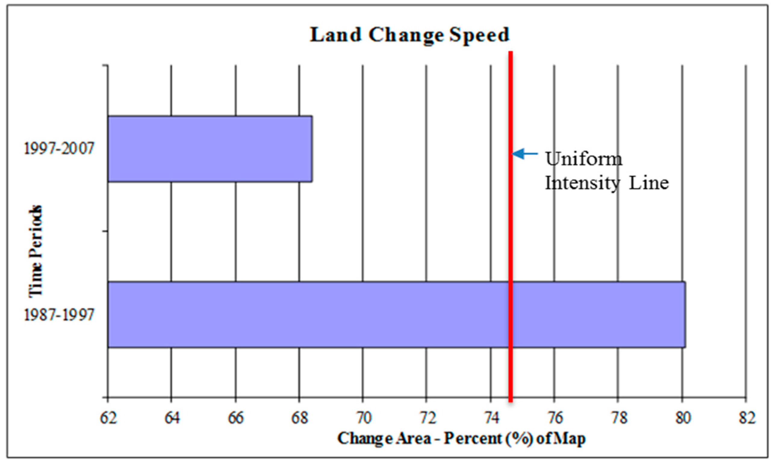
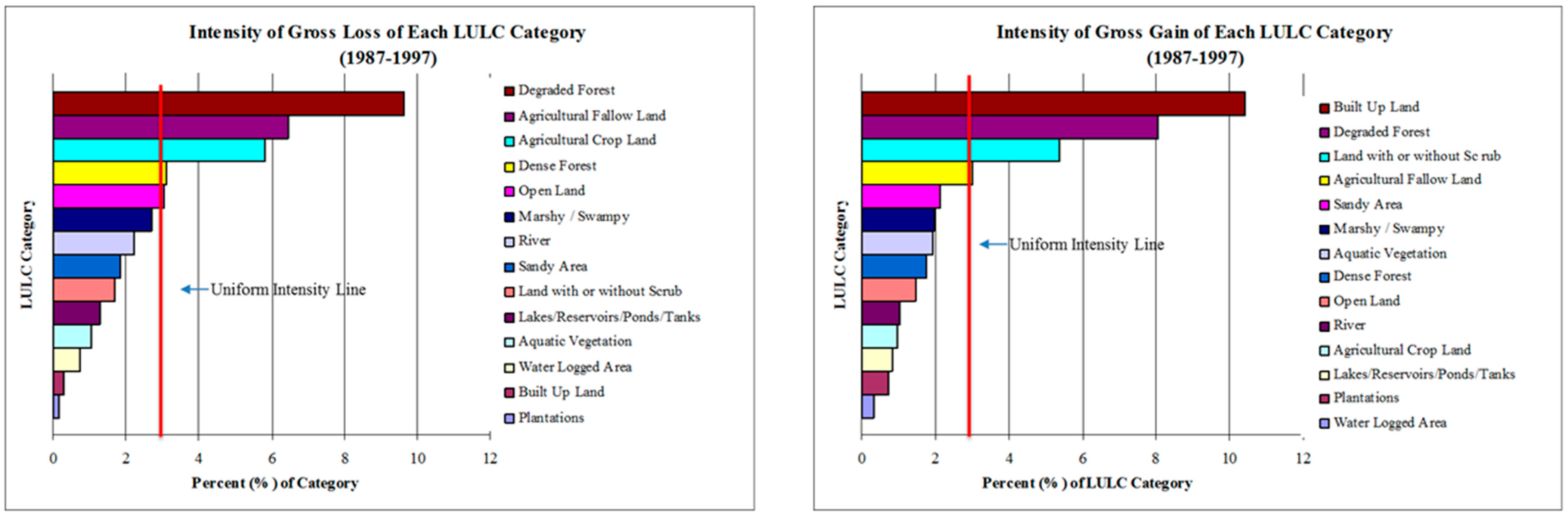
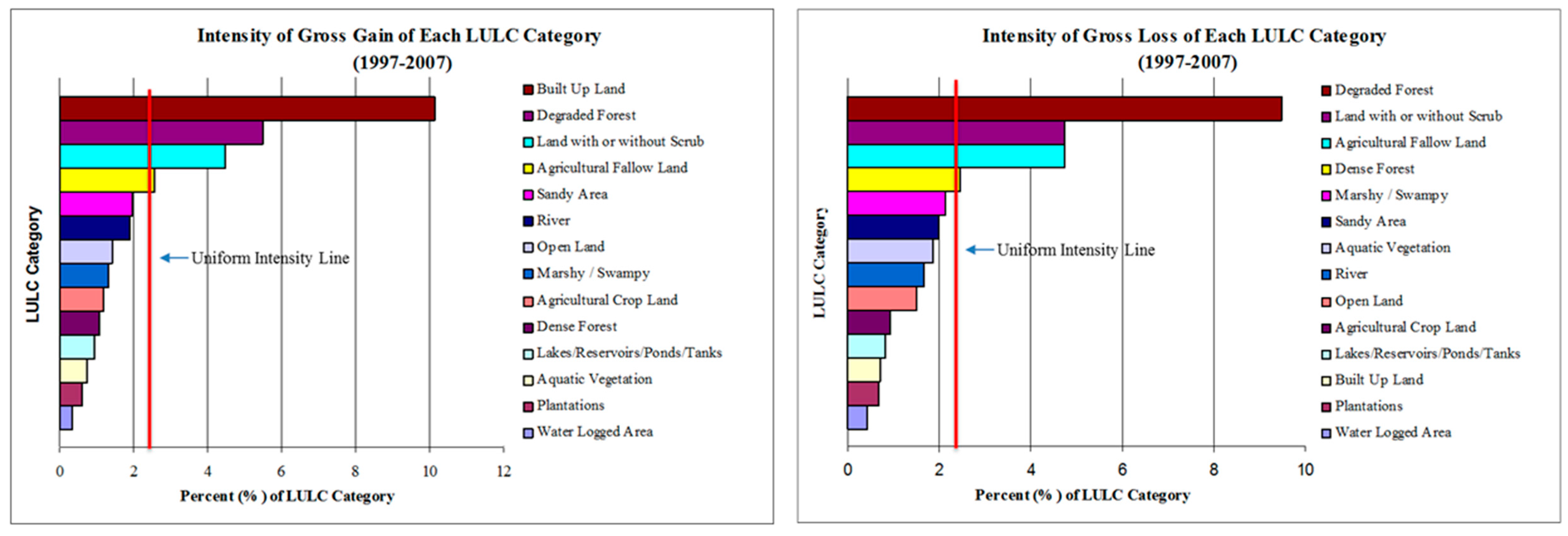
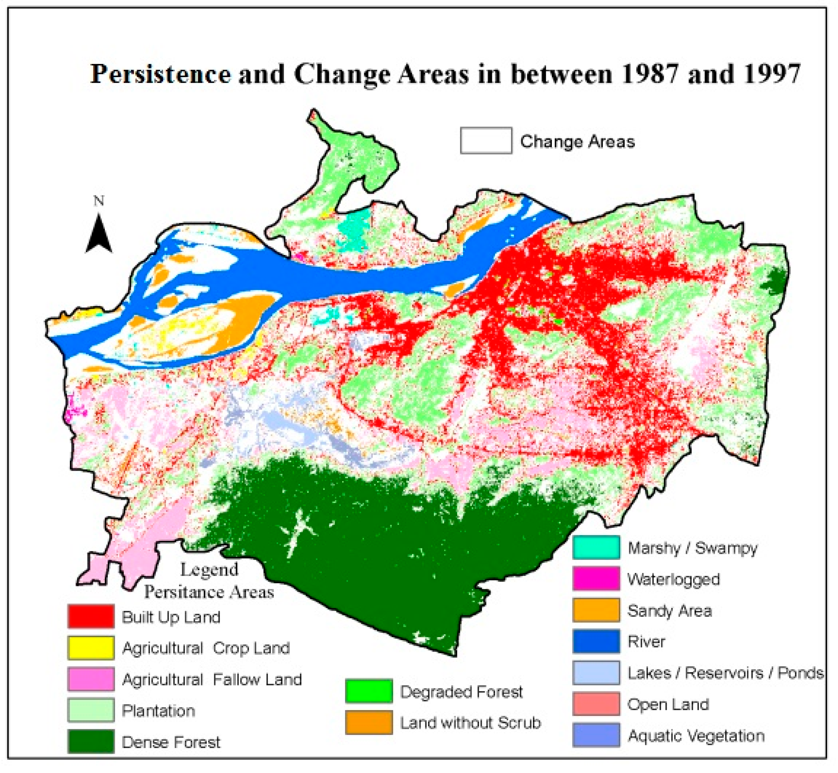
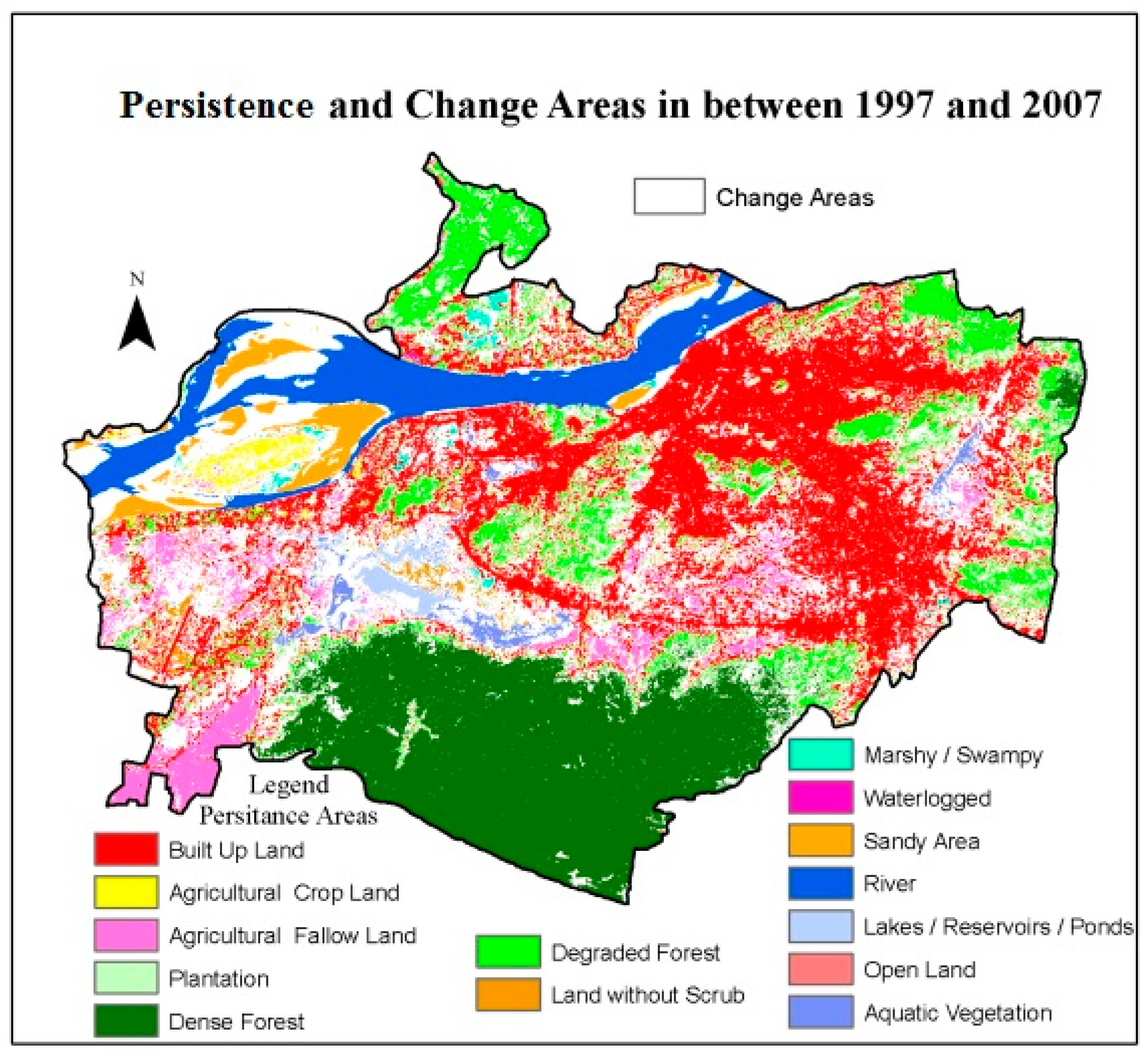
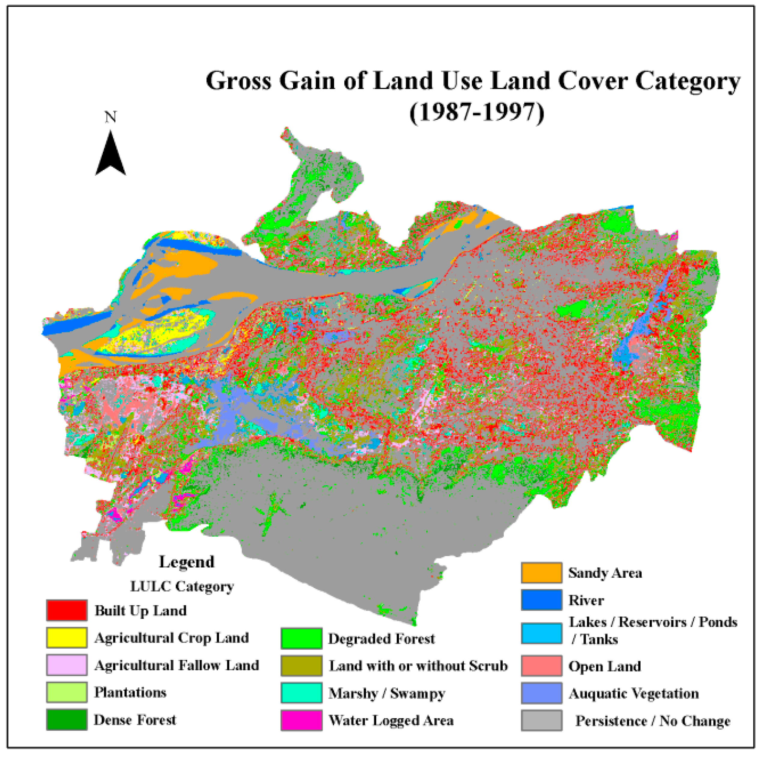
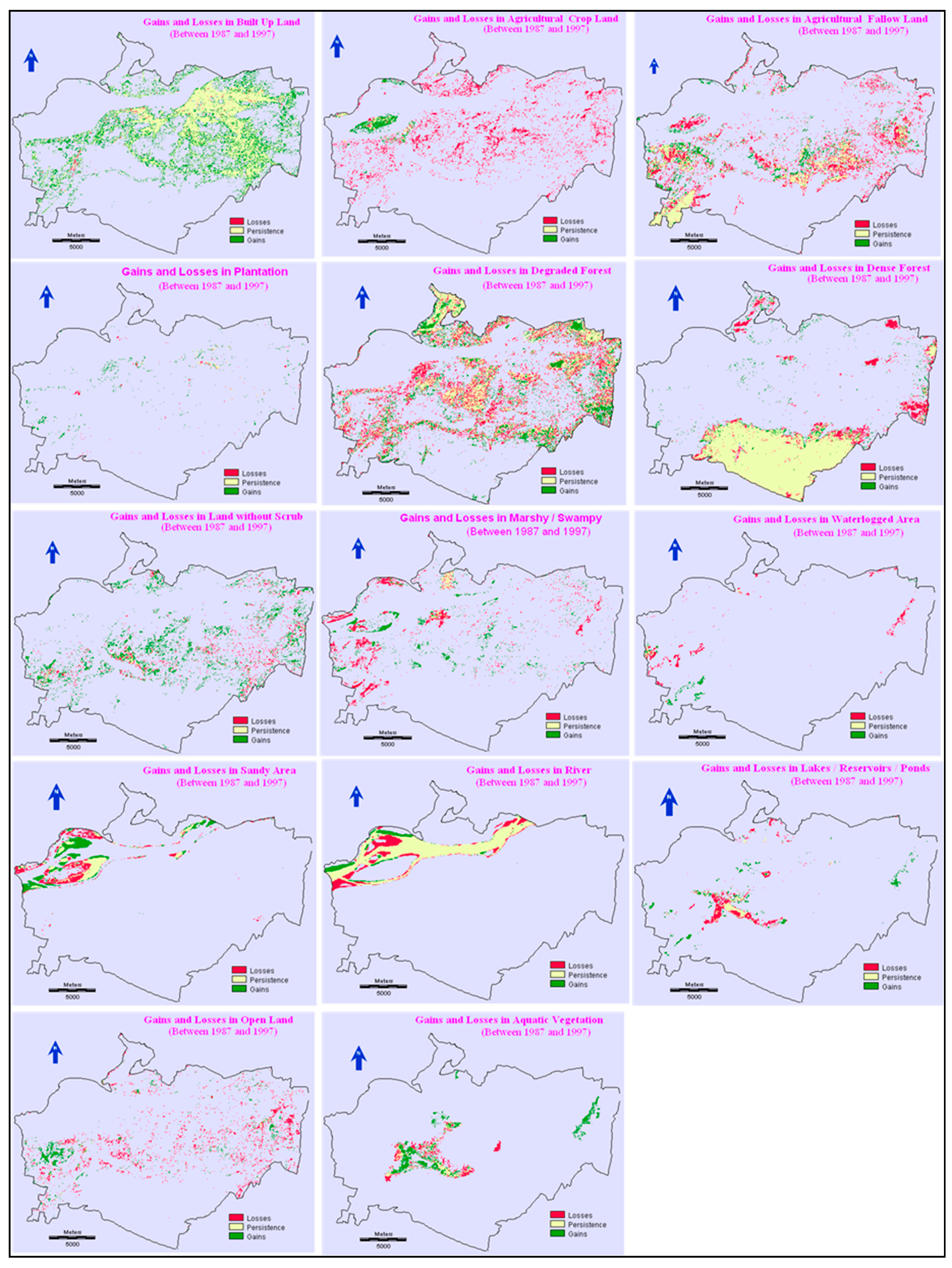
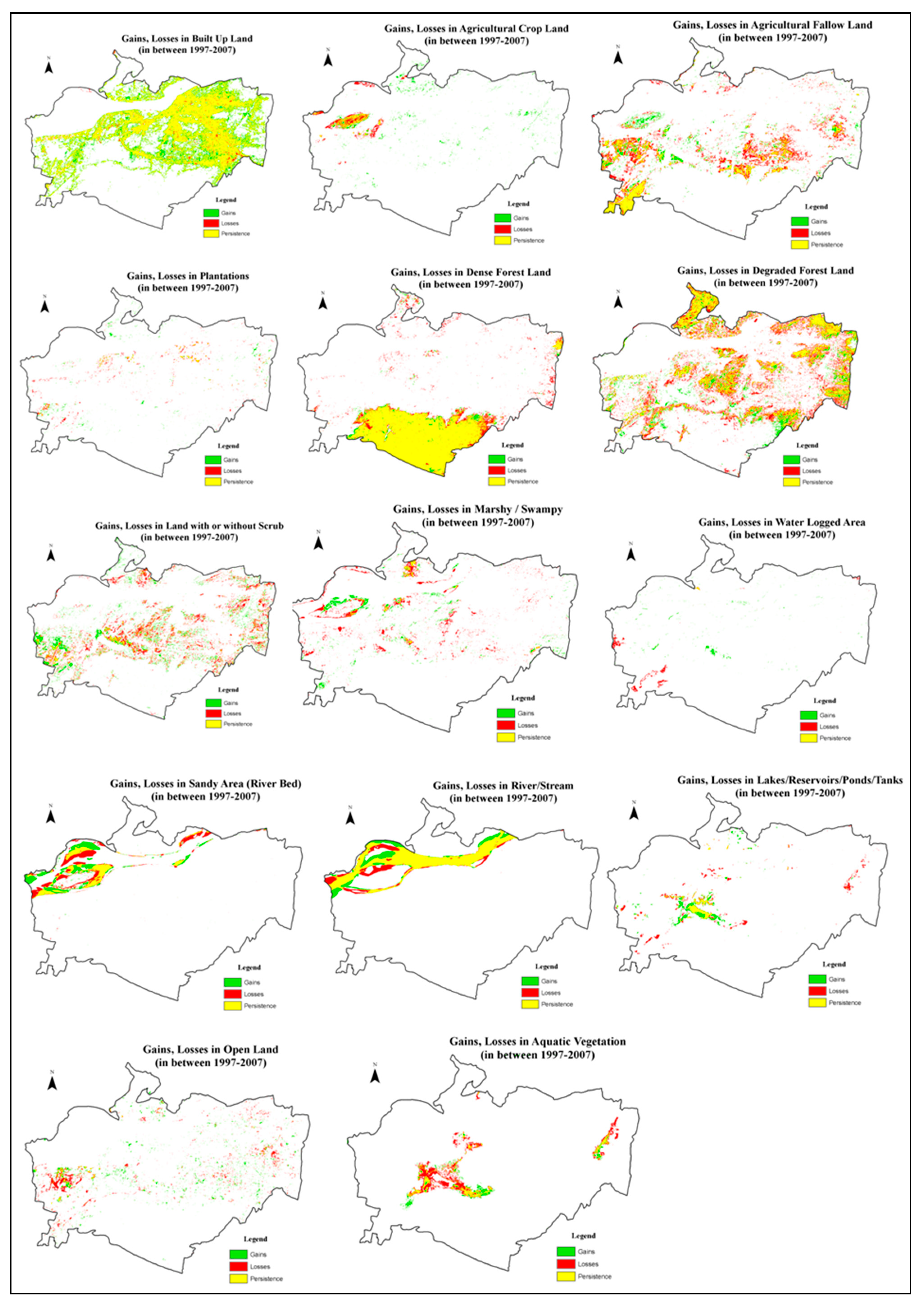
4.2.2. Gross Gain, Gross Loss, and Persistence in Quantity of LULC

| LULC in 1997 | LULC in 1987 | Total 1997 | Gross Gain | |||||||||||||
|---|---|---|---|---|---|---|---|---|---|---|---|---|---|---|---|---|
| Built up Land | Agricultural Crop Land | Agricultural Fallow Land | Plantations | Dense Forest | Degraded Forest/Scrub | Land with or without Scrub | Marshy/Swampy | Water Logged Area | Sandy Area (Riverbed) | River/Stream | Lake/Reservoir/Pond/Tank | Open Land | Aquatic Vegetation | |||
| Built up Land | 14.33 | 1.75 | 2.30 | 0.03 | 0.05 | 3.65 | 0.66 | 0.48 | 0.11 | 0.12 | 0.08 | 0.08 | 0.98 | 0.12 | 24.75 | 10.42 |
| Agricultural Crop Land | 0.00 | 0.46 | 0.40 | 0.00 | 0.00 | 0.07 | 0.00 | 0.15 | 0.00 | 0.33 | 0.01 | 0.00 | 0.01 | 0.00 | 1.44 | 0.98 |
| Agricultural Fallow Land | 0.00 | 0.71 | 5.21 | 0.00 | 0.01 | 0.69 | 0.19 | 0.36 | 0.14 | 0.14 | 0.00 | 0.03 | 0.60 | 0.15 | 8.23 | 3.02 |
| Plantations | 0.11 | 0.09 | 0.04 | 0.16 | 0.01 | 0.34 | 0.03 | 0.04 | 0.01 | 0.01 | 0.00 | 0.00 | 0.02 | 0.01 | 0.89 | 0.73 |
| Dense Forest | 0.00 | 0.06 | 0.05 | 0.03 | 17.71 | 1.52 | 0.03 | 0.03 | 0.00 | 0.00 | 0.00 | 0.01 | 0.02 | 0.01 | 19.48 | 1.77 |
| Degraded Forest | 0.06 | 1.65 | 1.29 | 0.06 | 2.82 | 10.54 | 0.56 | 0.48 | 0.08 | 0.05 | 0.04 | 0.11 | 0.66 | 0.16 | 18.58 | 8.04 |
| Land with or without Scrub | 0.00 | 0.98 | 0.94 | 0.01 | 0.19 | 2.31 | 0.61 | 0.11 | 0.03 | 0.02 | 0.00 | 0.06 | 0.48 | 0.25 | 5.99 | 5.38 |
| Marshy/Swampy | 0.03 | 0.21 | 0.40 | 0.00 | 0.01 | 0.45 | 0.05 | 0.52 | 0.02 | 0.44 | 0.12 | 0.02 | 0.12 | 0.08 | 2.48 | 1.96 |
| Water Logged Area | 0.00 | 0.01 | 0.10 | 0.00 | 0.00 | 0.08 | 0.00 | 0.12 | 0.10 | 0.00 | 0.00 | 0.01 | 0.01 | 0.02 | 0.45 | 0.35 |
| Sandy Area (River Bed) | 0.00 | 0.04 | 0.02 | 0.00 | 0.00 | 0.01 | 0.00 | 0.10 | 0.02 | 1.73 | 1.94 | 0.00 | 0.01 | 0.00 | 3.87 | 2.14 |
| River/Stream | 0.00 | 0.02 | 0.01 | 0.00 | 0.00 | 0.00 | 0.00 | 0.29 | 0.01 | 0.71 | 6.80 | 0.00 | 0.00 | 0.00 | 7.85 | 1.05 |
| Lake/Reservoir/Pond/Tank | 0.02 | 0.03 | 0.07 | 0.02 | 0.00 | 0.10 | 0.01 | 0.21 | 0.09 | 0.01 | 0.00 | 0.64 | 0.03 | 0.22 | 1.46 | 0.82 |
| Open Land | 0.05 | 0.12 | 0.70 | 0.00 | 0.01 | 0.16 | 0.05 | 0.16 | 0.12 | 0.02 | 0.01 | 0.03 | 0.29 | 0.03 | 1.76 | 1.47 |
| Aquatic Vegetation | 0.02 | 0.11 | 0.12 | 0.01 | 0.00 | 0.24 | 0.09 | 0.18 | 0.11 | 0.00 | 0.00 | 0.94 | 0.10 | 0.84 | 2.77 | 1.93 |
| 1997 Total | 14.63 | 6.26 | 11.65 | 0.34 | 20.81 | 20.16 | 2.29 | 3.24 | 0.86 | 3.59 | 9.02 | 1.93 | 3.34 | 1.88 | 100.00 | 40.06 |
| Gross Loss | 0.30 | 5.80 | 6.44 | 0.18 | 3.10 | 9.62 | 1.68 | 2.72 | 0.76 | 1.86 | 2.22 | 1.29 | 3.05 | 1.04 | 40.06 | |
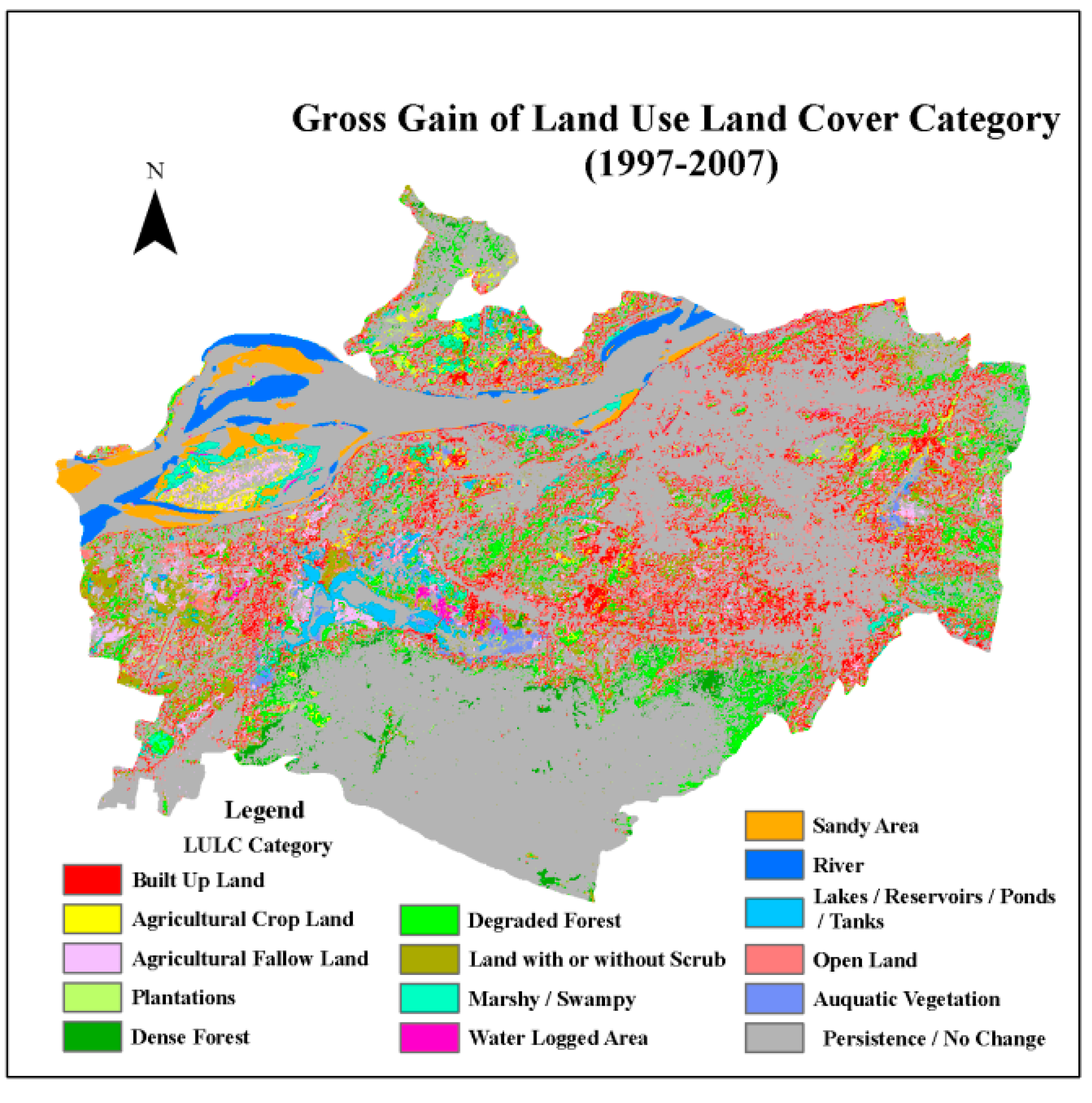
| LULC in 2007 | LULC in 1997 | Total 1997 | Gross Gain | |||||||||||||
|---|---|---|---|---|---|---|---|---|---|---|---|---|---|---|---|---|
| Built Up Land | Agricultural Crop Land | Agricultural Fallow Land | Plantations | Dense Forest | Degraded Forest | Land with or without Scrub | Marshy/Swampy | Water Logged Area | Sandy Area (Riverbed) | River/Stream | Lake/Reservoir/Pond/Tank | Open Land | Aquatic Vegetation | |||
| Built Up Land | 24.05 | 0.14 | 1.97 | 0.39 | 0.24 | 4.30 | 1.41 | 0.50 | 0.06 | 0.08 | 0.05 | 0.15 | 0.53 | 0.30 | 34.17 | 10.12 |
| Agricultural Crop Land | 0.01 | 0.53 | 0.17 | 0.03 | 0.05 | 0.40 | 0.17 | 0.14 | 0.01 | 0.10 | 0.00 | 0.02 | 0.01 | 0.09 | 1.73 | 1.20 |
| Agricultural Fallow Land | 0.03 | 0.34 | 3.49 | 0.02 | 0.02 | 0.57 | 0.52 | 0.36 | 0.03 | 0.08 | 0.00 | 0.05 | 0.42 | 0.13 | 6.07 | 2.58 |
| Plantations | 0.02 | 0.02 | 0.05 | 0.21 | 0.11 | 0.22 | 0.11 | 0.01 | 0.01 | 0.00 | 0.00 | 0.02 | 0.00 | 0.03 | 0.81 | 0.60 |
| Dense Forest | 0.00 | 0.00 | 0.00 | 0.00 | 16.99 | 1.03 | 0.04 | 0.00 | 0.00 | 0.00 | 0.00 | 0.00 | 0.00 | 0.01 | 18.07 | 1.08 |
| Degraded Forest | 0.14 | 0.04 | 0.67 | 0.13 | 1.80 | 9.08 | 2.02 | 0.27 | 0.09 | 0.01 | 0.00 | 0.05 | 0.10 | 0.17 | 14.58 | 5.50 |
| Land with or without Scrub | 0.07 | 0.05 | 1.07 | 0.07 | 0.16 | 1.93 | 1.25 | 0.26 | 0.13 | 0.02 | 0.00 | 0.16 | 0.27 | 0.29 | 5.73 | 4.48 |
| Marshy/Swampy | 0.04 | 0.06 | 0.09 | 0.02 | 0.04 | 0.39 | 0.07 | 0.33 | 0.05 | 0.28 | 0.13 | 0.07 | 0.04 | 0.05 | 1.66 | 1.33 |
| Water Logged Area | 0.00 | 0.00 | 0.04 | 0.00 | 0.01 | 0.09 | 0.05 | 0.01 | 0.02 | 0.03 | 0.03 | 0.02 | 0.03 | 0.03 | 0.37 | 0.35 |
| Sandy Area (River Bed) | 0.01 | 0.11 | 0.06 | 0.00 | 0.00 | 0.02 | 0.01 | 0.28 | 0.00 | 1.88 | 1.45 | 0.01 | 0.01 | 0.00 | 3.84 | 1.96 |
| River/Stream | 0.04 | 0.13 | 0.06 | 0.00 | 0.00 | 0.05 | 0.01 | 0.19 | 0.00 | 1.41 | 6.18 | 0.00 | 0.00 | 0.00 | 8.07 | 1.89 |
| Lake/Reservoir/Pond/Tank | 0.02 | 0.00 | 0.04 | 0.00 | 0.01 | 0.08 | 0.03 | 0.02 | 0.01 | 0.00 | 0.00 | 0.63 | 0.03 | 0.70 | 1.57 | 0.94 |
| Open Land | 0.31 | 0.02 | 0.45 | 0.01 | 0.02 | 0.25 | 0.15 | 0.08 | 0.01 | 0.00 | 0.00 | 0.03 | 0.26 | 0.08 | 1.67 | 1.41 |
| Aquatic Vegetation | 0.01 | 0 | 0.08 | 0.01 | 0.01 | 0.15 | 0.16 | 0.03 | 0.04 | 0 | 0.00 | 0.24 | 0.03 | 0.90 | 1.66 | 0.76 |
| 1997 Total | 24.76 | 1.45 | 8.23 | 0.89 | 19.45 | 18.56 | 6.00 | 2.48 | 0.45 | 3.88 | 7.86 | 1.46 | 1.76 | 2.77 | 100 | 34.20 |
| Gross Loss | 0.71 | 0.92 | 4.74 | 0.68 | 2.46 | 9.48 | 4.75 | 2.15 | 0.43 | 2.00 | 1.68 | .83 | 1.50 | 1.87 | 34.20 | |
| Land Use/Land Cover Class | Persistence | Gain | Loss | Total Change (Gain + Loss) | Value of Net Change (Gain − Loss) | Absolute Value of Net Change (Gain − Loss) | Swap (Total Change—Absolute Value of Net Change) |
|---|---|---|---|---|---|---|---|
| Built up Land | 14.33 | 10.42 | 0.30 | 10.72 | 10.12 | 10.12 | 0.60 |
| Agricultural Crop Land | 0.46 | 0.98 | 5.80 | 6.78 | −4.82 | 4.82 | 1.96 |
| Agricultural Fallow Land | 5.21 | 3.02 | 6.44 | 9.46 | −3.42 | 3.42 | 6.04 |
| Plantations | 0.16 | 0.73 | 0.18 | 0.91 | 0.55 | 0.55 | 0.36 |
| Dense Forest | 17.71 | 1.77 | 3.10 | 4.87 | −1.33 | 1.33 | 3.54 |
| Degraded Forest | 10.54 | 8.04 | 9.62 | 17.66 | −1.58 | 1.58 | 16.08 |
| Land with or without Scrub | 0.61 | 5.38 | 1.68 | 7.06 | 3.7 | 3.7 | 3.36 |
| Marshy/Swampy | 0.52 | 1.96 | 2.72 | 4.68 | −0.76 | 0.76 | 3.92 |
| Water Logged Area | 0.1 | 0.35 | 0.76 | 1.11 | −0.41 | 0.41 | 0.70 |
| Sandy Area (River Bed) | 1.73 | 2.14 | 1.86 | 4.00 | 0.28 | 0.28 | 3.72 |
| River/Stream | 6.8 | 1.05 | 2.22 | 3.27 | −1.17 | 1.17 | 2.10 |
| Lake/Reservoir/Pond/Tank | 0.64 | 0.82 | 1.29 | 2.11 | −0.47 | 0.47 | 1.64 |
| Open Land | 0.29 | 1.47 | 3.05 | 4.52 | −1.58 | 1.58 | 2.94 |
| Aquatic Vegetation | 0.84 | 1.93 | 1.04 | 2.97 | 0.89 | 0.89 | 2.08 |
| Total | 59.94 | 40.06 | 40.06 | 80.12 | 0.0 | 31.08 | 49.04 |
| Land use/Land Cover Class | Persistence | Gain | Loss | Total Change (Gain + Loss) | Value of Net Change (Gain − Loss) | Absolute Value of Net Change (Gain − Loss) | Swap (Total Change—Absolute Value of Net Change) |
|---|---|---|---|---|---|---|---|
| Built ip Land | 24.05 | 10.12 | 0.71 | 10.83 | 9.41 | 9.41 | 1.42 |
| Agricultural Crop Land | 0.53 | 1.2 | 0.92 | 2.12 | 0.28 | 0.28 | 1.84 |
| Agricultural Fallow Land | 3.49 | 2.58 | 4.74 | 7.32 | –2.16 | 2.16 | 5.16 |
| Plantations | 0.21 | 0.6 | 0.68 | 1.28 | –0.08 | 0.08 | 1.2 |
| Dense Forest | 16.99 | 1.08 | 2.46 | 3.54 | –1.38 | 1.38 | 2.16 |
| Degraded Forest | 9.08 | 5.5 | 9.48 | 14.98 | –3.98 | 3.98 | 11 |
| Land with or without Scrub | 1.25 | 4.48 | 4.75 | 9.23 | –0.27 | 0.27 | 8.96 |
| Marshy/Swampy | 0.33 | 1.33 | 2.15 | 3.48 | –0.82 | 0.82 | 2.66 |
| Water Logged Area | 0.02 | 0.35 | 0.43 | 0.78 | –0.08 | 0.08 | 0.7 |
| Sandy Area (River Bed) | 1.88 | 1.96 | 2 | 3.96 | –0.04 | 0.04 | 3.92 |
| River/Stream | 6.18 | 1.89 | 1.68 | 3.57 | 0.21 | 0.21 | 3.36 |
| Lake/Reservoir/Pond/Tank | 0.63 | 0.94 | 0.83 | 1.77 | 0.11 | 0.11 | 1.66 |
| Open Land | 0.26 | 1.41 | 1.5 | 2.91 | –0.09 | 0.09 | 2.82 |
| Aquatic Vegetation | 0.9 | 0.76 | 1.87 | 2.63 | –1.11 | 1.11 | 1.52 |
| Total | 65.8 | 34.2 | 34.2 | 68.4 | 0.0 | 20.02 | 48.38 |
4.2.3. Net Change and Swap Changes in Quantity of LULC

| Land Use/Land Cover Class | Gain | Land Use/Land Cover Class | Loss | Land Use/Land Cover Class | Total Change (Gain+ Loss) | Land Use/Land Cover Class | Persistence |
|---|---|---|---|---|---|---|---|
| Built up Land | 10.42 | Degraded Forest | 9.62 | Degraded Forest | 17.66 | Dense Forest | 17.71 |
| Degraded Forest | 8.04 | Agricultural Fallow Land | 6.44 | Built Up Land | 10.72 | Built Up Land | 14.33 |
| Land with or without Scrub | 5.38 | Agricultural Crop Land | 5.8 | Agricultural Fallow Land | 9.46 | Degraded Forest | 10.54 |
| Agricultural Fallow Land | 3.02 | Dense Forest | 3.1 | Land with or without Scrub | 7.06 | River/Stream | 6.8 |
| Sandy Area (River Bed) | 2.14 | Open Land | 3.05 | Agricultural Crop Land | 6.78 | Agricultural Fallow Land | 5.21 |
| Marshy/Swampy | 1.96 | Marshy/Swampy | 2.72 | Dense Forest | 4.87 | Sandy Area (River Bed) | 1.73 |
| Aquatic Vegetation | 1.93 | River/Stream | 2.22 | Marshy/Swampy | 4.68 | Aquatic Vegetation | 0.84 |
| Dense Forest | 1.77 | Sandy Area (River Bed) | 1.86 | Open Land | 4.52 | Lake/Reservoir/Pond/Tank | 0.64 |
| Open Land | 1.47 | Land with or without Scrub | 1.68 | Sandy Area (River Bed) | 4 | Land with or without Scrub | 0.61 |
| River/Stream | 1.05 | Lake/Reservoir/Pond/Tank | 1.29 | River/Stream | 3.27 | Marshy/Swampy | 0.52 |
| Agricultural Crop Land | 0.98 | Aquatic Vegetation | 1.04 | Aquatic Vegetation | 2.97 | Agricultural Crop Land | 0.46 |
| Lake/Reservoir/Pond/Tank | 0.82 | Water Logged Area | 0.76 | Lake/Reservoir/Pond/Tank | 2.11 | Open Land | 0.29 |
| Plantations | 0.73 | Built Up Land | 0.3 | Water Logged Area | 1.11 | Plantations | 0.16 |
| Water Logged Area | 0.35 | Plantations | 0.18 | Plantations | 0.91 | Water Logged Area | 0.1 |
| Total | 40.06 | 40.06 | 80.12 | 59.94 |
| Land Use/Land Cover Class | Gain | Land Use/Land Cover Class | Loss | Land Use/Land Cover Class | Total Change (Gain + Loss) | Land Use/Land Cover Class | Persistence |
|---|---|---|---|---|---|---|---|
| Built up Land | 10.12 | Degraded Forest | 9.48 | Degraded Forest | 14.98 | Built Up Land | 24.05 |
| Degraded Forest | 5.5 | Land with or without Scrub | 4.75 | Built Up Land | 10.83 | Dense Forest | 16.99 |
| Land with or without Scrub | 4.48 | Agricultural Fallow Land | 4.74 | Land with or without Scrub | 9.23 | Degraded Forest | 9.08 |
| Agricultural Fallow Land | 2.58 | Dense Forest | 2.46 | Agricultural Fallow Land | 7.32 | River/Stream | 6.18 |
| Sandy Area (River Bed) | 1.96 | Marshy/Swampy | 2.15 | Sandy Area (River Bed) | 3.96 | Agricultural Fallow Land | 3.49 |
| River/Stream | 1.89 | Sandy Area (River Bed) | 2 | River/Stream | 3.57 | Sandy Area (River Bed) | 1.88 |
| Open Land | 1.41 | Aquatic Vegetation | 1.87 | Dense Forest | 3.54 | Land with or without Scrub | 1.25 |
| Marshy/Swampy | 1.33 | River/Stream | 1.68 | Marshy/Swampy | 3.48 | Aquatic Vegetation | 0.9 |
| Agricultural Crop Land | 1.2 | Open Land | 1.5 | Open Land | 2.91 | Lake/Reservoir/Pond/Tank | 0.63 |
| Dense Forest | 1.08 | Agricultural Crop Land | 0.92 | Aquatic Vegetation | 2.63 | Agricultural Crop Land | 0.53 |
| Lake/Reservoir/Pond/Tank | 0.94 | Lake/Reservoir/Pond/Tank | 0.83 | Agricultural Crop Land | 2.12 | Marshy/Swampy | 0.33 |
| Aquatic Vegetation | 0.76 | Built Up Land | 0.71 | Lake/Reservoir/Pond/Tank | 1.77 | Open Land | 0.26 |
| Plantations | 0.6 | Plantations | 0.68 | Plantations | 1.28 | Plantations | 0.21 |
| Water Logged Area | 0.35 | Water Logged Area | 0.43 | Water Logged Area | 0.78 | Water Logged Area | 0.02 |
| Total | 34.2 | 34.2 | 68.4 | 65.8 |


| Swap Ranking between 1987 and 1997 | Swap Ranking between 1997 and 2007 | |||
|---|---|---|---|---|
| Swap | LULC Class | LULC Class | Swap | |
| 16.08 | Degraded Forest | Degraded Forest | 11 | |
| 6.04 | Agricultural Fallow Land | Land with or without Scrub | 8.96 | |
| 3.92 | Marshy/Swampy | Agricultural Fallow Land | 5.16 | |
| 3.72 | Sandy Area (River Bed) | Sandy Area (River Bed) | 3.92 | |
| 3.54 | Dense Forest | River/Stream | 3.36 | |
| 3.36 | Land with or without Scrub | Open Land | 2.82 | |
| 2.94 | Open Land | Marshy/Swampy | 2.66 | |
| 2.1 | River/Stream | Dense Forest | 2.16 | |
| 2.08 | Aquatic Vegetation | Agricultural Crop Land | 1.84 | |
| 1.96 | Agricultural Crop Land | Lake/Reservoir/Pond/Tank | 1.66 | |
| 1.64 | Lake/Reservoir/Pond/Tank | Aquatic Vegetation | 1.52 | |
| 0.7 | Water Logged Area | Built up Land | 1.42 | |
| 0.6 | Built Up Land | Plantations | 1.2 | |
| 0.36 | Plantations | Water Logged Area | 0.7 | |
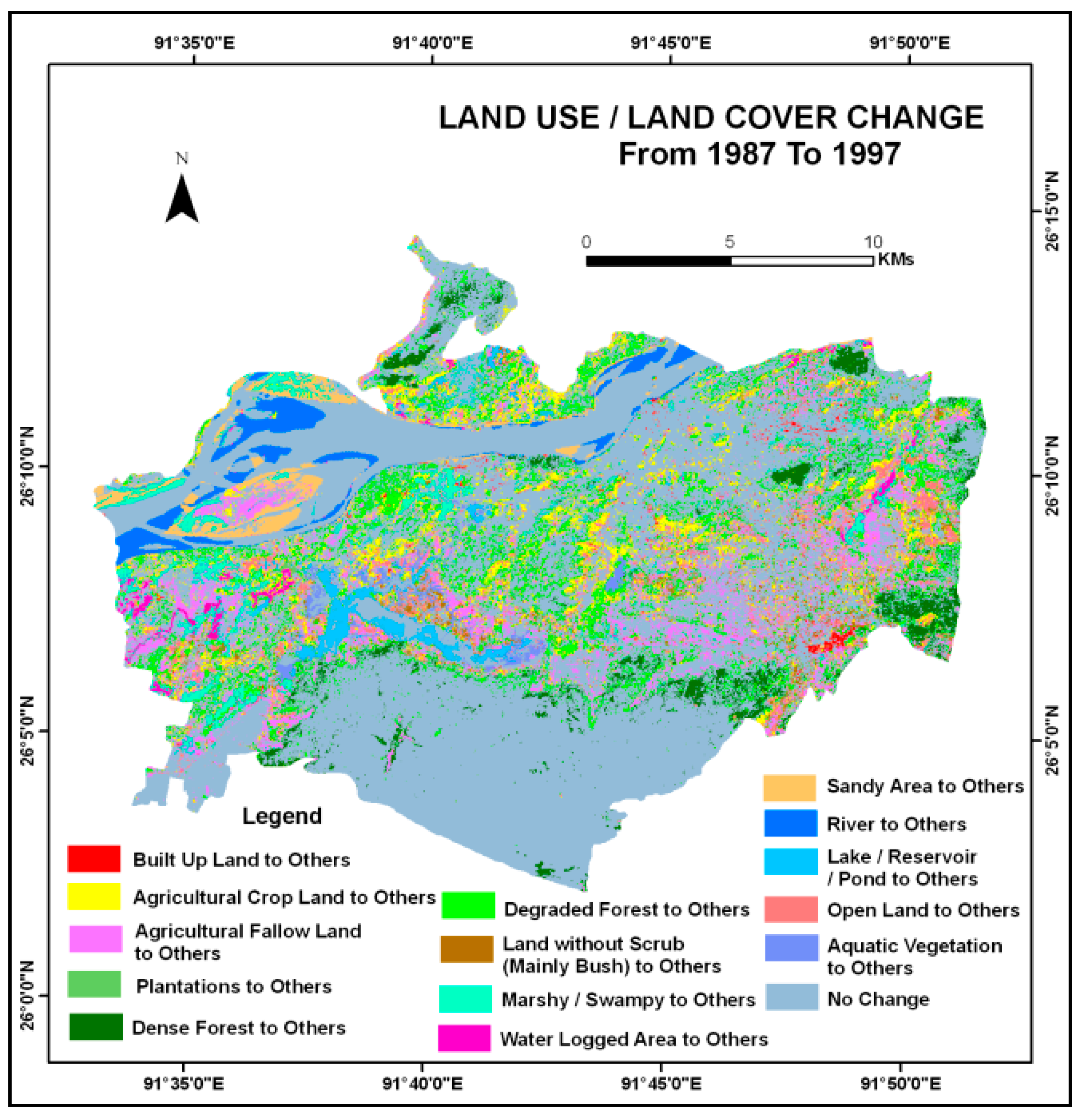
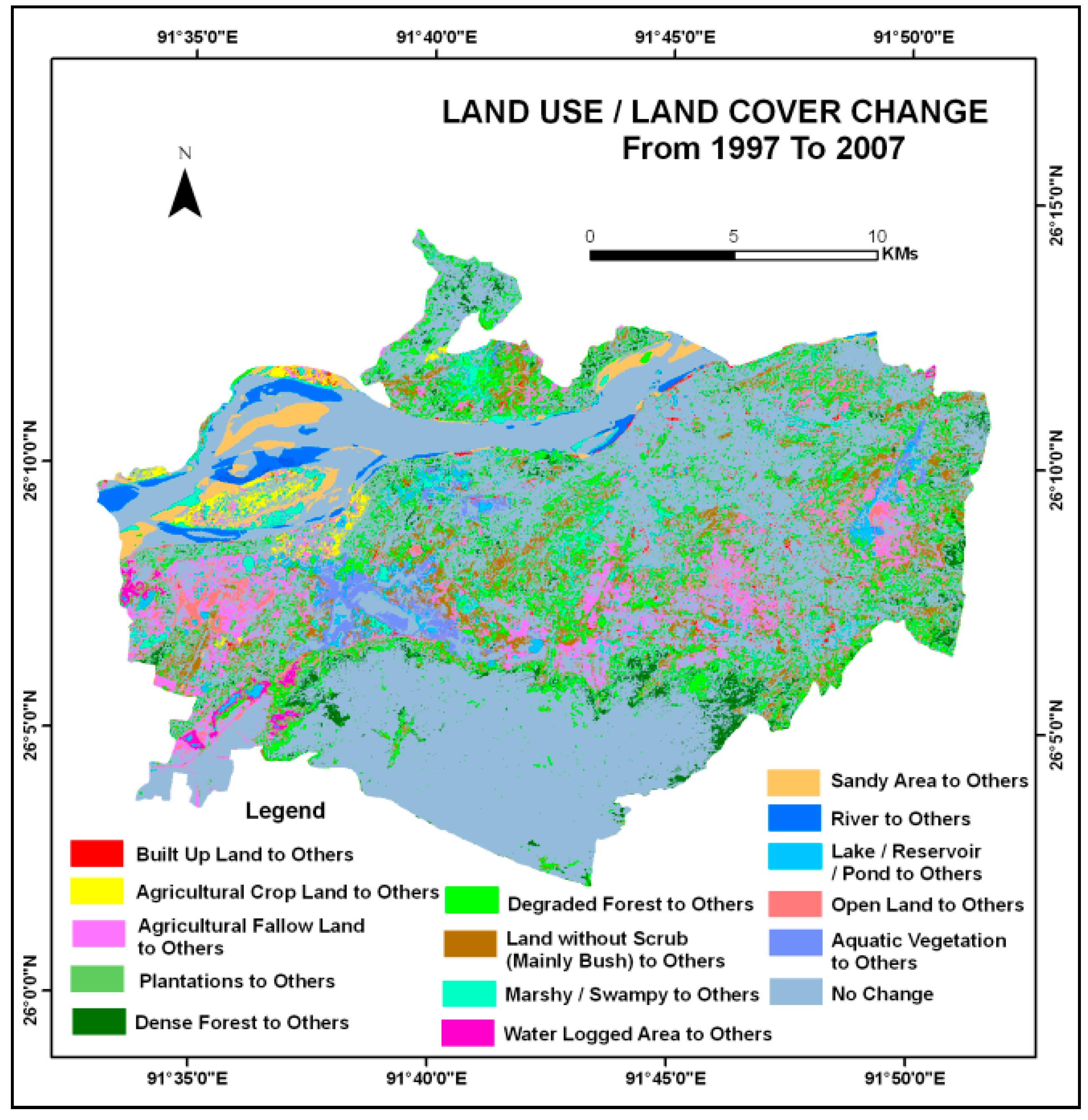
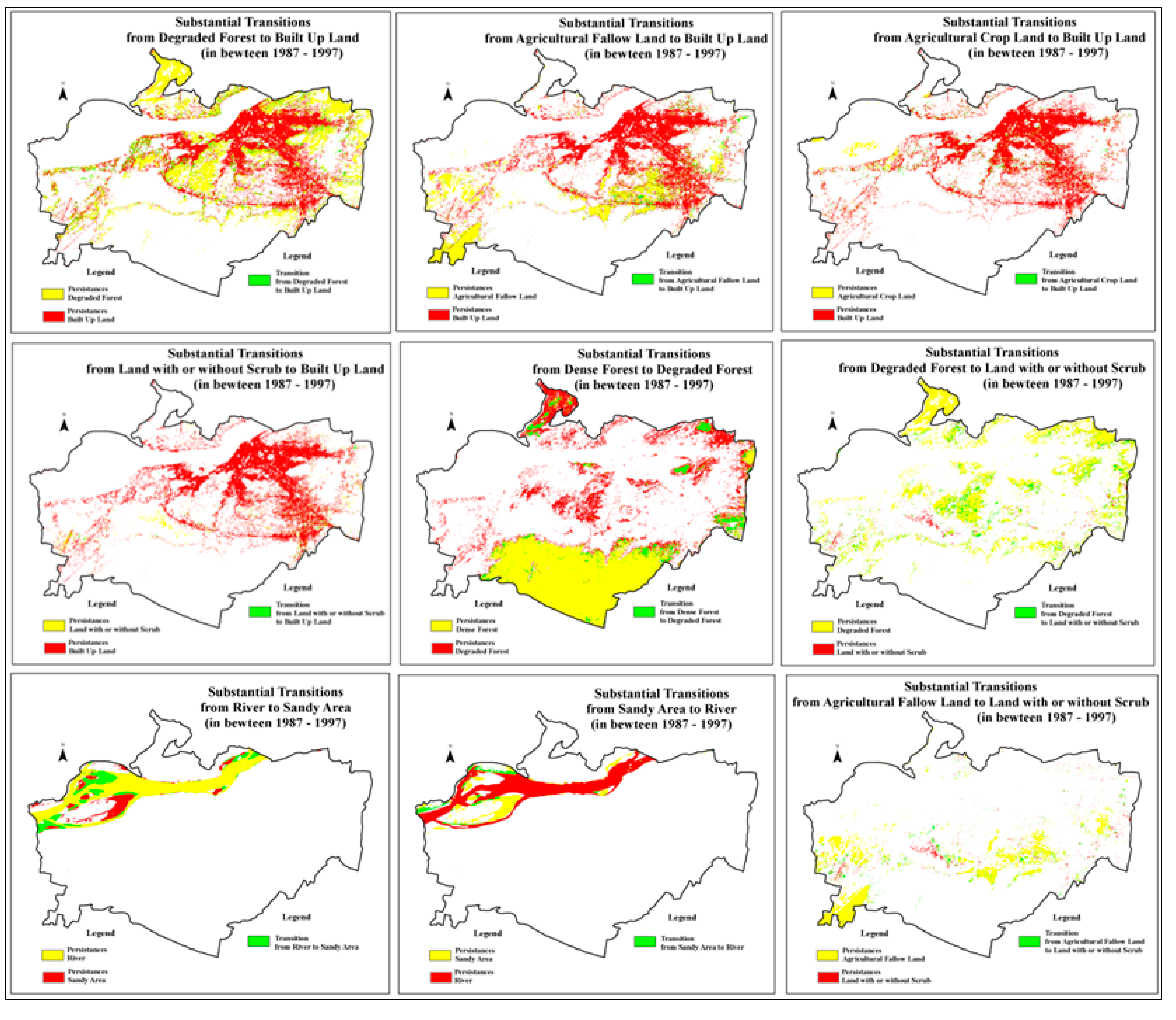
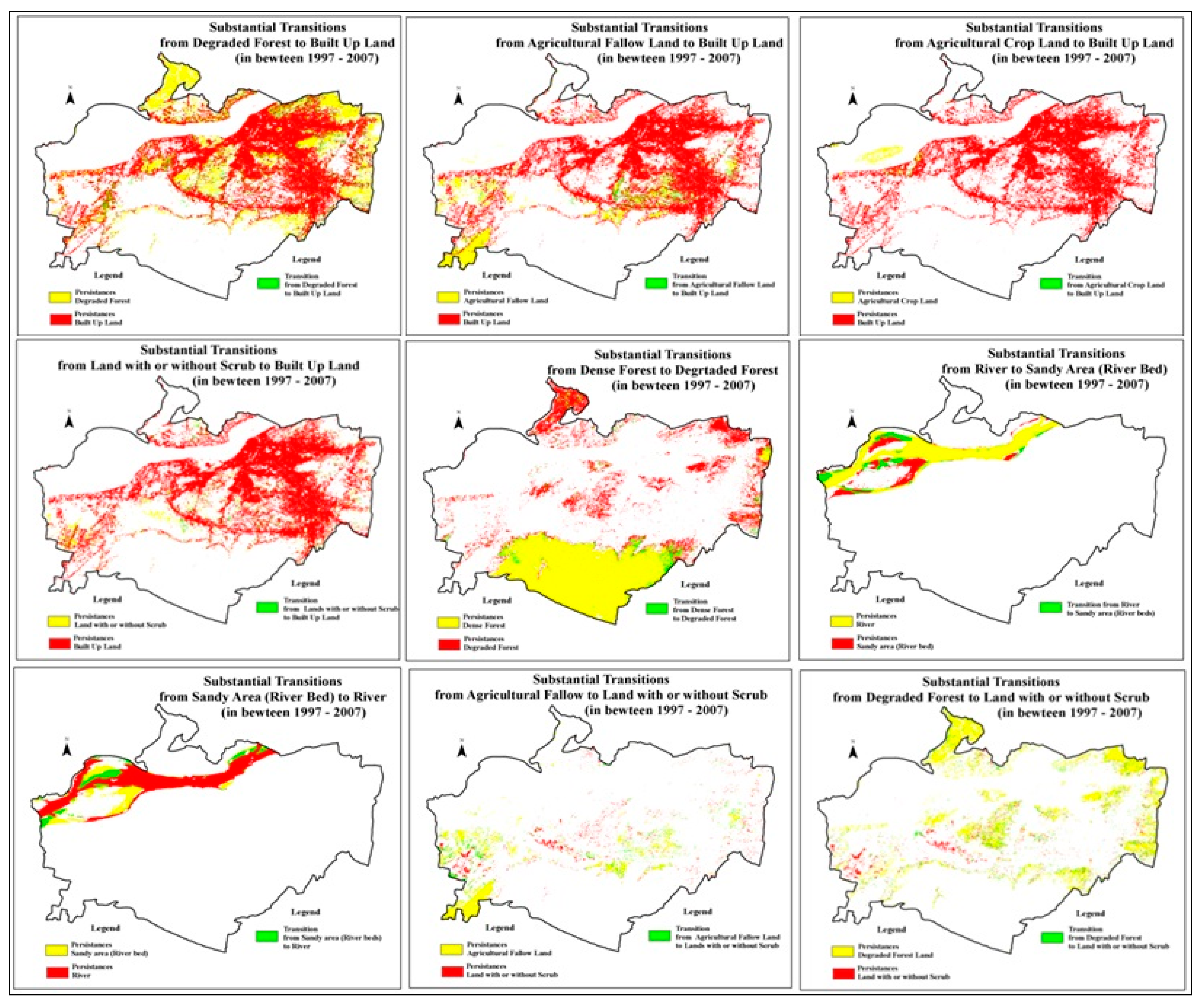
4.3. Changes in Allocation of LULC


| LULC | Time Periods | ||
|---|---|---|---|
| Change from | Change to | 1987–1997 | 1997–2007 |
| Degraded Forest | Built up | 3.65% | 4.30% |
| Agricultural Fallow Land | Built up | 2.30% | 1.97% |
| Agricultural Crop Land | Built up | 1.75% | 0.14% |
| Dense | Degraded | 2.82% | 1.80% |
| Degraded Forest | Land with or without Scrub | 2.31% | 0.16% |
| Land with or without Scrub | Built up | 0.66% | 1.41% |
| River | River Bed | 1.94% | 1.45% |
| River Bed (Sandy Area) | River | - | 1.41% |
| Agricultural Fallow Land | Land with or without Scrub | - | 1.07% |
5. Conclusions
Author Contributions
Conflicts of Interest
References
- Asselman, N.E.M.; Middelkoop, H. Floodplain sedimentation: Quantities, patterns and processes. Earth Surf. Process. Landf. 1995, 20, 481–499. [Google Scholar] [CrossRef]
- Aboel Ghar, M.; Shalaby, A.; Ryutaro, T. Agricultural LandMonitoring in the Egyptian Nile Delta using landsat data. Int. J. Environ. Stud. 2004, 1, 651–657. [Google Scholar]
- Erasoab, N.R.; Armenteras-Pascualb, D.; Alumbrerosa, J.R. Land use and land cover change in the Colombian Andes: Dynamics and future scenarios. J. Land Use Sci. 2012, 8, 154–174. [Google Scholar]
- Turner, B.L., II; David, S.; Steven, S.; Fischer, G.; Fresco, L.; Leemans, R. Land-Use and Land-Cover Change: Science/Research Plan; IGBP Report No. 35 and HDP Report No. 7; International Geosphere-Biosphere Programme and the Human Dimensions of Global Environmental Change Programme: Stockholm, Sweden, 1995. [Google Scholar]
- William, E.R.; William, B.M.; Turner, B.L., II. Modeling land use and land cover as part of global environmental change. Clim. Change 1994, 28, 45–64. [Google Scholar] [CrossRef]
- Meyer, W.B.; Turner, B.L., II. Human population growth and global land-use/cover change. Ann. Rev. Ecol. System. 1994, 23, 39–61. [Google Scholar] [CrossRef]
- Singh, A. Digital change detection techniques using remotely sensed data. Int. J. Remote Sens. 1989, 10, 989–1003. [Google Scholar] [CrossRef]
- Jensen, J.R. Introductory Digital Image Processing: A Remote Sensing Perspective; Prentice-Hall: Upper Saddle River, NJ, USA, 1996; p. 318. [Google Scholar]
- Mondal, M.S.; Nayan Sharma, N.; Kappas, M.; Garg, P.K. Modeling of spatio-temporal dynamics of land use and land cover in a part of Brahmaputra River basin using Geoinformatic techniques. Geocarto Int. 2013, 28, 632–656. [Google Scholar] [CrossRef]
- Pontius, R.G., Jr.; Shusas, E.; Mceachern, M. Detecting important categorical land changes while accounting for persistence. Agric. Ecosys. Environ. 2004, 101, 251–268. [Google Scholar] [CrossRef]
© 2015 by the authors; licensee MDPI, Basel, Switzerland. This article is an open access article distributed under the terms and conditions of the Creative Commons Attribution license (http://creativecommons.org/licenses/by/4.0/).
Share and Cite
Mondal, M.S.; Sharma, N.; Kappas, M.; Garg, P.K. Critical Assessment of Land Use Land Cover Dynamics Using Multi-Temporal Satellite Images. Environments 2015, 2, 61-90. https://0-doi-org.brum.beds.ac.uk/10.3390/environments2010061
Mondal MS, Sharma N, Kappas M, Garg PK. Critical Assessment of Land Use Land Cover Dynamics Using Multi-Temporal Satellite Images. Environments. 2015; 2(1):61-90. https://0-doi-org.brum.beds.ac.uk/10.3390/environments2010061
Chicago/Turabian StyleMondal, Md. Surabuddin, Nayan Sharma, Martin Kappas, and P. K. Garg. 2015. "Critical Assessment of Land Use Land Cover Dynamics Using Multi-Temporal Satellite Images" Environments 2, no. 1: 61-90. https://0-doi-org.brum.beds.ac.uk/10.3390/environments2010061