Joule Heating Effects in Electrokinetic Remediation: Role of Non-Uniform Soil Environments: Temperature Profile Behavior and Hydrodynamics

Abstract

Electrokinetic remediation is a process in which a low-voltage direct-current electric field is applied across a section of contaminated soil to remove contaminants. In this work, the effect of Joule heating on the heat transfer and hydrodynamics aspects in a non-uniform environment is simulated. The proposed model is based on a rectangular capillary with non-symmetrical heat transfer conditions similar to those found in non-uniform soil environments. The mathematical and microscopic model described here uses two key parameters in addition to the Nusselt number: the ratio between the Nusselt numbers calculated at both walls of the capillary, named R, and a function of this variable and the Nusselt number, indicated by F(R, Nu). Illustrations describing the five key regimens for the system behavior are presented in terms of ranges for R and F(R, Nu) values, which indicate the key role of the parameter R in controlling the behaviors of the temperature and velocity profiles. Prediction, analysis, and illustration of five different regimes of flow complete the study, and conclusions are given to illustrate how the behavior of the system is affected.

1. Introduction

Electrokinetic remediation, also termed electrokinetic soil cleaning, is a technique that uses direct electrical fields to remove organic, inorganic, and heavy metal particles from the soil by the use of an electric potential [1]. One of the advantages of this technique is that it provides an approach with minimum disturbance to the soil matrix while helping to clean subsurface contaminants. It is based on the application of an electric field directly to the contaminated soil site. The effect of the applied electric field helps transport species (contaminants) to a common place from where they are then removed from the soil and collected from the electrodes (anode and/or cathode) [2,3].

In addition, the electrokinetic remediation technique is preferred due to other attractive characteristics that include lower costs, less exposure to the contaminants, adaptability to different types of soils, and less disturbance of the environment, i.e., soil matrix [4]. However, the effectiveness and efficiency of the operation depends on the stratification and permeability of soil. In contrast, ex-situ technologies related to remediation processes such as soil washing allow for better control of the operation; also, the remediation results are not strongly affected by soil characteristics such as stratification and permeability [5,6]. However, the current ex-situ technologies have an extra cost due to the fact that the affected area is removed from its original place and relocated to a new place, the processing equipment is expensive, and the perturbation of soil matrix is important to a degree that it is no longer suitable for agricultural use without additional preconditioning [7].

The electrokinetic-based technique, in general, displays Joule heating effects since, as a result of applying voltage, it leads to the generation of heat due to the electrical resistance of the soil. The analysis of the Joule heating effects (on both temperature and the hydrodynamic velocity profiles of the system) is an important aspect that needs further study for the purpose of a better scaling and design of the technology.

This is the subject matter of the study reported in this paper. Fostering an understanding of how Joule heating affects temperature and hydrodynamic velocity profiles in electrokinetic soil cleaning will lead to more effective protocols in the soil treatment of contaminated sites [8,9,10].

The research in this paper focuses on soils with potential non-uniform properties across the soil matrix. Previously, Boland et al. [11] studied Joule heating effects on electrokinetic remediation using a cylindrical capillary to capture the most important aspects of its behavior. The cylindrical geometry, however, cannot capture situations that are not symmetrical without additional complexity. The study reported in this paper, however, has selected a capillary domain with a rectangular geometry, which has an intrinsic characteristic of easily accommodating non-symmetrical boundary conditions and allowing an effective study by simplifying the problem [12,13]. A very limited analysis of the potential effect of two different environmental temperatures on hydrodynamics was reported by Oyanader et al. [14], who also used a rectangular geometry for the capillary domains.

In this paper, we present a complete analysis of the effect of non-symmetrical conditions (at the capillary boundaries) on both temperature and hydrodynamic velocity profiles. These non-symmetrical properties can emerge from possible non-uniformities of soils due to composition, humidity, concentration of contaminants, etc. These non-uniformities can generate different heat transfer conditions at the boundaries of a domain which, in turn, will lead to non-symmetrical boundary conditions and generate different “local” behaviors of hydrodynamic flows within the capillary as well [14,15]. Understanding these effects is very important in order to gain insights into the potential design and implementation of the cleaning strategies of the soils [16,17].

The objective of the present work is to explore the effects of Joule heating on the behavior of heat transfer systems (i.e., temperature profiles) and hydrodynamic velocity profiles found in non-uniform soil environments. In order to keep the analysis mathematically simple, we assume that the soil surface charges are negligible so that the presence of electroosmosis within the capillary domain can be ignored [14]. This model leads to the identification of a number of heat transfer “regimes” which, in turn, control several types of flow regimes within the capillary. Each of these regimes shows a characteristic velocity profile with a typical behavior. Details of the model formulation, solutions, and numerical illustrations are given in the sections below.

2. Problem Formulation of the Heat Transfer Model

Figure 1 is a sketch of the system under analysis. This system consists of a rectangular capillary of length L, width H, depth W and an inclination of an angle α (0–90°) with respect to the orientation of gravity “g”. Also, in this analysis, a case of dominant heat conduction is assumed in the direction to fluid flow, i.e., the hypothesis proposed by Bachelor, and that it is valid for moderate values of the Grash of number [18]. The pore domain is viewed as a typical pore in a porous medium where the energy source, i.e., the Joule heating, is a volumetric and homogeneous source with constant values across the bulk of such domain. It is also worth noting that the coordinates “x” and “y” have been anchored coincidently at the lower corner of the capillary channel. This location helps to coordinate the calculation of the hydrodynamic velocity profile [19].

Under the assumptions that soils can be viewed as porous media, that they can be modeled by a set of capillaries [20], and that the rectangular geometry of these capillaries is useful for the study of non-uniform (soil) properties, this section describes a heat transfer model for this geometrical domain with Joule heating generation. This model assumes the presence of different Nusselt numbers along the walls of the capillary in order to investigate to role of the non-uniform heat transfer properties for the heat releasing from Joule heating generation. It should be noted that the conditions of the heat transfer (out of the capillary domain) at each wall will be described by a generalized boundary condition (i.e., Robin type), which includes conduction and convection only. Due to the fact that the temperature ranges normally used in the electrokinetic process are relatively low, compared to conditions in furnaces, for example, the radiation may be neglected. The objective of this model is to determine the behavior of the temperature profiles under a variation of the heat transfer parameters as suggested by different Nusselt numbers. This information is very useful for the hydrodynamic model of the system in order to determine the hydrodynamic velocity profile of the capillary domain. As in Boland et al. [11], our objective is to present the most general study with respect to the Joule heating effects on both the temperature and hydrodynamic profiles.

The energy equation for the case of the conduction-driven regime that is dominant within the capillary domain is given by Bird et al. [21]:

$$k{\nabla }^{2}T+Q=0$$

(1)

This equation applied to the domain of Figure 1 in rectangular coordinates is then written as:

$$k[\frac{{\partial }^{2}T}{\partial x^2}+\frac{{\partial }^{2}T}{\partial y^2}]+Q=0$$

(2)

where Joule heating generation can be viewed as:

$$\frac{dq}{dt}=I^2\times \mathbf{R}\equiv Q$$

(3)

In Equation (3), “I” indicates power, and the notation R indicates the electrical resistance of the physical domain. Q specifies the generation of heat due to Joule heating [22]. As mentioned before, the function Q is assumed uniform and constant within the bulk of the domain of the capillary. The thermal conductivity of the capillary domain is given by k, the temperature is represented by T (x,y) which is a function of x and y within the domain of the capillary. The direction “z” (see Figure 1) is not relevant because we assume “symmetry” in that direction. Also for the domain, geometry is assumed that L >> H and W >> H. From the geometric point of view, the domain can be thought as of a bounded domain with two parallel surfaces, one located at y = 0 and the other one, at y = H.

The energy Equation (2) can be transformed into a dimensionless form by defining non-dimensional variables as follows:

$$\widehat{x}=\frac{x}{L},\eta =\frac{y}{H},\Theta =\frac{T-T_{\infty }}{T_{\infty }}$$

(4)

Substituting these new dimensionless variables in Equation (2) and by using the assumption H/L << 1, as well as the dimensionless heat generation number results in the following:

$${\Phi }^2=\frac{Q{H}^2}{k{T}_{\infty }}$$

(5)

The following differential, non-dimensional equation for the energy conservation can be written:

$$\frac{d^2\Theta }{d{\eta }^2}=-{\Phi }^2$$

(6)

Using the following boundary condition:

$$\begin{array}{l}{-k\frac{dT}{dy}|}_{wallH}=h_H({T|}_{y=H}-T_{\infty })\\ {-k\frac{dT}{dy}|}_{wall0}=h_0({T|}_{y=0}-T_{\infty })\end{array}$$

(7)

where h_H and h₀ have been used to indicate heat transfer coefficients at the position y = H and y = 0, respectively. Now, by following dimensionless variables defined in Equation (4), Equation (7) becomes:

$$\begin{array}{l}{\frac{-d\Theta }{d\eta }|}_{\eta =0}={Nu\Theta |}_{\eta =0}\\ {\frac{-d\Theta }{d\eta }|}_{\eta =1}={RNu\Theta |}_{\eta =1}\end{array}$$

(8)

where Nu is generally used to indicate the Nusselt number given by [21]:

$$Nu\equiv \frac{hL}{k}$$

(9)

Also, by defining the R ratio as:

$$R\equiv \frac{N{u}^1}{N{u}^0},\to N{u}^1=RN{u}^0$$

(10)

where $N{u}^0$ is used to indicate the Nusselt number along the wall located at $\eta =0$ while $N{u}^1$ represents the Nusselt number at the opposite wall ($\eta =1$).

3. Formulation of the Hydrodynamic Model

The formulation and solution of the hydrodynamic problem, including the calculation of the velocity profile, follows the Systematic and Integrative Sequence Approach (SISA) for mastery learning [23] that consists of the following key steps:

(1)

Identifying Geometry: The geometry used in this study is of rectangular shape with dimensions L, H, W (Figure 1).

(2)

Selection of the Coordinate System: The coordinate system is “anchored” in one of the vertices of the capillary domain to simplify the calculation of the flow rate (or flow) (Figure 1).

(3)

Kinematics of Flow: Components of the velocity profile are described. Therefore, for the case under analysis:

a.

$V_x\ne 0$ (the flow of the fluid is in the axial direction only since ends effects are neglected)

b.

$V_y=0$ (there is no net flow perpendicular to the axial flow in the domain)

c.

$V_z=0$ (there is no net flow in the direction perpendicular to the xy plane of the domain)

Based on the description above, we can postulate that the hydrodynamics is given by

$\underset{V}{\to }$ (v_z, 0, 0) as the unidimensional vector.

(4)

Boussinesq Approximation: This approximation uses the incompressibility condition everywhere except in the buoyancy term [24]. By using this approximation, all the effects of temperature on the system and due to Joule heating are considered only in the density variation with the temperature. Other properties such as viscosity and the heat capacity are considered constant in the model equations. Basically, the fluid behaves as incompressible, i.e., as it is assumed that there is no density variation in the case of conservation of total mass and, therefore, the continuity equation with the divergence of the vector field equated to zero is valid. This condition leads to the following conclusion:

$$V_x=f(y)$$

(11)

because (additionally) it assumed symmetry in the coordinate “z”.

(5)

Application of the Conservation of Momentum: Since the buffer is assumed to exhibit Newtonian fluid behavior, the Navier-Stokes equation is valid [21]. In the axial flow direction and with the assumption indicate above, the Navier-Stokes equation for the x-component is:

$$-\mu \frac{d^2{V}_x}{d{y}^2}=\frac{\partial p}{\partial x}+\rho (T)g_x$$

(12)

To determine the component, the density variation with the temperature, ρ (T), is required. This function is derived from the Taylor approximation to first order for a medium temperature; it is given by Bird et al. [21]

$$\rho (T)=\overline{\rho }-\overline{\rho }\beta (T-\overline{T)}$$

(13)

By substituting the equation above into the dimensional Navier Stokes equation the following equation is obtained:

$$\mu \frac{d^2{V}_x}{d{y}^2}=-\rho \beta g\sin (\alpha )(T-\overline{T)}$$

(14)

Alternatively, the non-dimensional form:

$$\frac{d^2{V}_x}{d{\eta }^2}=-Gr\sin (\alpha )[\Theta (\eta )-\overline{\Theta }]$$

(15)

Table 1. Summary of the Differential Hydrodynamic Models for Velocity Profile.

a. Non dimensional Navier Stokes equation and boundary conditions [21]:
$\frac{d^2{V}_x}{d{\eta }^2}=-Gr\sin (\alpha )[\Theta (\eta )-\overline{\Theta }]$	(16)
$V_x(\eta =0)=V_x(\eta =1)=0$	(17)
b. Non dimensional function of density and temperature derived from the Taylor approximation [21]:
$\frac{\rho (\Theta )}{\overline{\rho }}=1-\beta (\Theta -\overline{\Theta })$	(18)
c. Heat transfer model, where the function is defined by:
$F(R,Nu)\equiv \frac{(RNu+2)}{(1+R+RNu)}$	(19)
d. Non dimensional total mass conservation [21]:
${\displaystyle \underset{0}{\overset{1}{\int }}\rho (\overline{\Theta })V_x(\eta )d\eta =0}$	(20)
e. Mean value theorem for integration:
${\displaystyle \underset{0}{\overset{1}{\int }}{V}_x(\eta )d\eta =0}$	(21)

summarizes the hydrodynamic model for capillary rectangular geometry.

4. Solution and Obtaining Both the Heat Transfer and Velocity Profile Equations

4.1. Solution to Differential Model: The Distinct Heat Transfer Regimes

According to the Heat transfer regimes, the general solution to the differential equation (see Equation (22)) is given by:

$$\Theta (\eta )=-\frac{{\Phi }^2{\eta }^2}{2}+C_1\eta +C_2|$$

(22)

where C₁ and C₂ are +integration constants. These constants can be determined using the boundary conditions (8) to find that:

$$C_1=\frac{Nu{\Phi }^2(\frac{RNu}{2}+1)}{Nu+R(N{u}^2+Nu)}$$

(23)

$$C_2=\frac{{\Phi }^2(\frac{RNu}{2}+1)}{Nu+R(N{u}^2+Nu)}$$

(24)

However, these constants C₁ and C₂ can be rewritten as:

$$C_1=\frac{{\Phi }^2}{2}F(R,Nu)$$

(25)

$$C_2=\frac{{\Phi }^2}{2Nu}F(R,Nu)$$

(26)

where the factor F(R, Nu) has been defined as (see above Equation (19)):

After some algebraic manipulations, the general solution can be written as:

$${\theta }_r(\eta )=\frac{-{\eta }^2}{2}+\left(\frac{F(R,Nu)}{2}\right)\eta +\frac{1}{Nu}$$

(27)

where the non-dimensional and “reduced temperature” ${\theta }_r(\eta )$ has been defined as ${\theta }_r(\eta )=\frac{\Theta (\eta )}{{\Phi }^2}$.

This variable tremendously simplifies the analysis since it is not an explicit function of the generation due to Joule heating. In short, this characteristic of the system allows the study to be valid for all possible cases of the Joule heating parameter. In other words, the value defined in Equation (6) is a “universal scaling parameter” for the temperature profile. This can be viewed as a “self-similar” parameter of the system where all the results (parametrically with Joule heating) are collapsed into a general equation.

Based on the values that the perimeter R and the function F(R, Nu) can take, it is possible to define five distinct cases of heat transfer and hydrodynamic regimes (

Table 2. General and Limiting Cases of Heat Transfer and Hydrodynamic Regimes Based on the Parameter R Values.

Case	R-Value	F-Value	Description	Comments (Heat Transfer Regime)	Comments (Hydrodynamic Regime)
1	1	F(R, Nu) = 1	Symmetrical (limiting) case with same Nu values at both boundaries	The profile will have a “symmetrical” shape with the maximum temperature located at the center of the capillary	The velocity profile will have a “symmetrical” shape with the maximum velocity (upward) located at the center of the capillary
2	0	F(R, Nu) = 2	Adiabatic (limiting) case at the wall located at $\eta =1$	The temperature located will be located at the boundary located at $\eta =1$	The velocity profile will show two regions: one upward positioned near the boundary located at $\eta =1$ and the other one downward, located near the wall. at $\eta =0$
3	∞	F(R, Nu) = Nu/(1 + Nu)	Well-mixed (limiting) case at the wall located at $\eta =1$	The temperature at the wall located at $\eta =1$ will reach the environmental temperature	The velocity profile will show two regions: One upward located near at the wall at $\eta =0$ and the other downward located near the wall at $\eta =1$
4	R > 1	$F(R,Nu)\equiv \frac{(RNu+2)}{(1+R+RNu)}$	General case where the boundary at $\eta =1$ has a “favorable” heat transfer rate than the one at $\eta =0$	These cases will show temperature profiles similar to Case 3 but the temperature will not reach the environmental one	These cases will show hydrodynamic velocity profiles with behaviors between Case 1 and Case 3
5	R < 1	$F(R,Nu)\equiv \frac{(RNu+2)}{(1+R+RNu)}$	General case where the boundary at $\eta =1$ has an “unfavorable” heat transfer rate than the one at $\eta =0$	The general shape of the temperature profiles will follow Case 2 showing a “slower” heat transfer rate at $\eta =1$	These cases will show hydrodynamic velocity profiles with behaviors between Case 2 and Case 1

).

4.2. Solution and Obtaining the Velocity Profile Equation

After the Navier Stokes equation has been identified (see Equation (16)), the equation requires the information related to the temperature profile, see Equation (22), that is the non-dimensional temperature profile. This relation leads to the fact that Equation (16) is a function of Joule heating and constant C₁ and C₂, of which are functions of the R and Nu numbers. C₁ and C₂ are given by Equations (23) and (24). This transformation gives the following modified Navier-Stokes equation as a function of the Grashof number, Gr, the Joule heating number, ${\Phi }^2$, and the medium temperature $\overline{\Theta }$ that will be determined later in Section 5 (see below):

$$\frac{d^2{V}_x}{d{\eta }^2}=\frac{{\Phi }^2}{2}Gr\sin (\alpha ){\eta }^2-Gr\sin (\alpha )C_1\eta -Gr\sin (\alpha )C_2+Gr\sin (\alpha )\overline{\Theta }$$

(28)

where by defining the following parameters:

$$A(\alpha ,\Phi )=\frac{-{\Phi }^2}{2}Gr\sin (\alpha )$$

(29)

$$B(\alpha ,\Phi ,Nu,R)\equiv Gr\sin (\alpha )C_1$$

(30)

$$C(\overline{\Theta )}\equiv Gr\sin (\alpha )\left[\overline{\Theta }-C_2\right]$$

(31)

Equation (28) leads to the following compact version:

$$\frac{d^2{V}_x}{d{\eta }^2}=-A(\alpha ,\Phi ){\eta }^2-B(\alpha ,\Phi ,Nu,R)\eta -C(\overline{\Theta })$$

(32)

By solving Equation (32)

$$V_x{}^{\prime }(\eta )=-\frac{A}{3}{\eta }^3-\frac{B}{2}{\eta }^2-C(\overline{\Theta })+D_1$$

(33)

$$V_x(\eta )=-\frac{A}{12}{\eta }^4-\frac{B}{6}{\eta }^3-\frac{C(\overline{\Theta }){\eta }^2}{2}+D_1\eta +D_2$$

(34)

where D₁ and D₂ are two integration constants to be determined using the non-slip boundary conditions,

$$V_x(0)=0\to D_2=0$$

(35)

Applying $V_x(\eta =1)=0$, we arrive at:

$$D_1=\frac{A}{12}+\frac{B}{6}+\frac{C(\overline{\Theta })}{2}$$

(36)

Now substituting the Equations (35) and (36) in (34), we obtain the following hydrodynamics velocity profile:

$$V_x(\eta )=\frac{A}{12}(\eta -{\eta }^4)+\frac{B}{6}(\eta -{\eta }^3)+\frac{C(\overline{\Theta })}{2}(\eta -{\eta }^2)$$

(37)

Clearly, one can see that the two boundary conditions have been verified by confirming that $V_x(\eta =0)=0$ and $V_x(\eta =1)=0$.

Since the net flow by conservation of mass is assumed to be zero, and by using the total mass balance equation, we obtain the following:

$${\displaystyle \underset{0}{\overset{1}{\int }}\rho (\overline{\Theta })V_x(\eta )d\eta =0}$$

(38)

By using the mean value theorem for integrals, we can conclude that:

$${\displaystyle \underset{0}{\overset{1}{\int }}{V}_x(\eta )d\eta =0}$$

(39)

And finally, by using the profile given by the Equation (37), we have:

$${\displaystyle \underset{0}{\overset{1}{\int }}d{n}^{\prime }\left[\frac{A}{12}({\eta }^{\prime }-{\eta \prime }^4)+\frac{B}{6}({\eta }^{\prime }-{\eta \prime }^3)+\frac{C(\overline{\Theta })}{2}({\eta }^{\prime }-{\eta \prime }^2)\right]=0}$$

(40)

To simplify this equation, we can define the following integrals:

$${\widehat{I}}_1+{\widehat{I}}_2+{\widehat{I}}_3(\overline{\Theta })=0$$

(41)

where

$${\widehat{I}}_1\equiv {\displaystyle \underset{0}{\overset{1}{\int }}d{n}^{\prime }\left[\frac{A}{12}({\eta }^{\prime }-{\eta }^{\prime 4})\right]=\frac{A}{12}{\displaystyle \underset{0}{\overset{1}{\int }}d{n}^{\prime }(}{\eta }^{\prime }-{\eta \prime }^4)=\frac{A}{12}{I}_1}$$

(42)

$${\widehat{I}}_1\equiv {\displaystyle \underset{0}{\overset{1}{\int }}d{n}^{\prime }\left[\frac{B}{6}({\eta }^{\prime }-{\eta \prime }^3)\right]=\frac{B}{6}{\displaystyle \underset{0}{\overset{1}{\int }}d{n}^{\prime }(}{\eta }^{\prime }-{\eta }^{\prime 3})=\frac{B}{6}{I}_2}$$

(43)

$${\widehat{I}}_3(\overline{\Theta })\equiv {\displaystyle \underset{0}{\overset{1}{\int }}d{n}^{\prime }\left[\frac{C(\overline{\Theta })}{2}({\eta }^{\prime }-{\eta \prime }^2)\right]=\frac{C(\overline{\Theta })}{2}{\displaystyle \underset{0}{\overset{1}{\int }}d{n}^{\prime }(}{\eta }^{\prime }-{\eta }^{\prime 2})=\frac{C(\overline{\Theta })}{2}{I}_3}$$

(44)

And the following integrals are defined as

$$I_1\equiv {\displaystyle \underset{0}{\overset{1}{\int }}d{n}^{\prime }({\eta \prime }^4-{\eta }^{\prime })=\frac{3}{10}}$$

(45)

$$I_2\equiv {\displaystyle \underset{0}{\overset{1}{\int }}d{n}^{\prime }({\eta }^{\prime 3}-{\eta }^{\prime })=\frac{1}{4}}$$

(46)

$$I_3\equiv {\displaystyle \underset{0}{\overset{1}{\int }}d{n}^{\prime }({\eta }^{\prime 2}-{\eta }^{\prime })=\frac{1}{6}}$$

(47)

Introducing Equations (42)–(44) into Equation (41) using the definitions Equations (45)–(47), we arrive at the following simplified equation:

$$\frac{A}{12}{I}_1+\frac{B}{6}{I}_2+\frac{C(\overline{\Theta })}{2}{I}_3=0$$

(48)

With Equation (48) we are able to obtain $C(\overline{\Theta })$ which must satisfy:

$$C(\overline{\Theta })=-\frac{A}{6}\frac{I_1}{I_3}-\frac{1}{3}\frac{I_2}{I_3}$$

(49)

Using Equation (31) will be able to get the value of $\overline{\Theta }$ in terms of integrals I₁, I₂, y I₃ such as:

$$\overline{\Theta }=C_2-\frac{A/6}{Gr\sin (\alpha )}\frac{I_1}{I_3}-\frac{B/3}{Gr\sin (\alpha )}\frac{I_2}{I_3}$$

(50)

Therefore, by using Equations (37) and (50), the hydrodynamic velocity profile is given by the following equation:

$$V_x(\eta )=-\frac{{\Phi }^2}{24}Gr\sin (\alpha )(\eta -{\eta }^4)+\frac{Gr\sin (\alpha )C_1}{6}(\eta -{\eta }^3)+[\frac{3}{40}{\Phi }^{2}Gr\sin (\alpha )-\frac{1}{4}Gr\sin (\alpha )C_1](\eta -{\eta }^2)$$

(51)

Equation (51) can be transformed into a reduced velocity equation which has the advantage of being independent of the fluid properties and some of the geometrical characteristics. The reduced velocity may be defined as following:

$$V_{xr}(\eta )\equiv \frac{V_x(\eta )}{{\Phi }^{2}Gr\sin (\alpha )}=-\frac{1}{24}(\eta -{\eta }^4)+[\frac{1}{12}F(R,Nu)](\eta -{\eta }^3)+[\frac{3}{40}-\frac{1}{8}F(R,Nu)](\eta -{\eta }^2)$$

(52)

Clearly, Equation (52) is only a function of the R parameter as well as the Nusselt number through the F(R, Nu) function.

Based the values that the perimeter R and the function F(R, Nu) can take, it is possible to define five distinct cases of heat transfer and hydrodynamic regimes (Table 2).

From these five cases, the first three (Cases 1–3) are limiting cases for particular values of the parameter R. The other two cases (Cases 4 and 5) are cases are based on ranges of values of the parameter R.

• Case 1: Symmetrical case, (R = 1) i.e., both Nu values at the different walls are the same
• Case 2: Adiabatic case, (R = 0) at the wall positioned at $\eta =1$. No heat flux is present at this location.
• Case 3: Well-mixed case, (R → ∞) at the wall positioned at $\eta =1$. This case has an excellent heat transfer at the position.

Furthermore, there are two general cases (Cases 4 and 5) for which the velocity profile in the capillary system when the heat transfer flow in the $\eta =1$ is greater than the one at the wall located at position $\eta =0$, i.e., R > 1 (Case 4). The opposite case is possible when the heat transfer flow at position $\eta =1$ is lower than the one at the wall located at $\eta =0$, i.e., R < 1 (Case 5). In the section below, a general analysis of the different cases with numerical illustrations is presented.

5. Different Heat Transfer and Hydrodynamic Regimes: Analysis, Numerical Illustration, and Discussion

5.1. Case 1: Symmetrical Case

This case implies that the Nusselt numbers for both the capillary walls $\eta =0$, $\eta =1$ are identical, i.e., $N{u}^1=N{u}^0=Nu$. Case 1 applied to the heat transfer and hydrodynamic regimes is shown below.

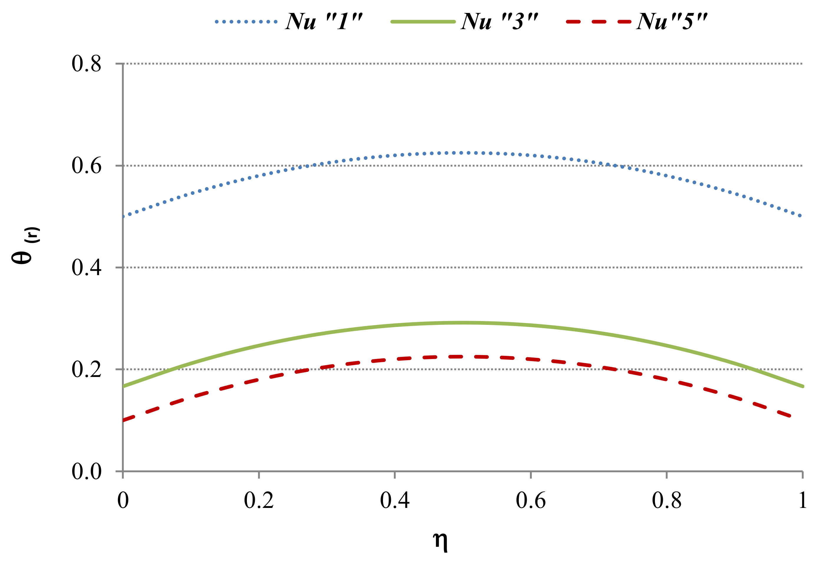
5.1.1. Case 1: Applied to the Heat Transfer Regime

Based on the general solution of the differential model (see Equation (22)), and the values presented in Table 2, one can write the following general solution of “reduced” temperature, ${\theta }_S^r(\eta )$ as:

$${\theta }_S^r(\eta )\equiv \frac{\Theta (\eta )}{{\Phi }^2}=-\frac{{\eta }^2}{2}+\frac{\eta }{2}+\frac{1}{2Nu}$$

(53)

Which is independent of parameter values ${\Phi }^2$, but has a dependency on the values of the Nusselt number (Nu). Clearly, as both heat fluxes in both capillary walls have the same value, the temperature profile ${\theta }_S^r(\eta )$ is symmetrical within the capillary domain (Figure 2). The special (in terms of Nu values) limiting case for extremely high values of Nusselt implies that:

$${({\theta }_S^r)}_{\infty }(\eta ){=}_{Nu}{\underrightarrow{\lim }}_{\infty }{\theta }_S^r{}_{(\eta )}=\eta (\frac{1}{2}-\frac{\eta }{2})$$

(54)

This function has a symmetrical shape around the axis $\eta =\frac{1}{2}$ with two minimum values located at both walls of the capillary, i.e., $\eta =0$ and $\eta =1$, respectively. Both of these values are given by ${\left({\theta }_S^r\right)}_{\infty }{}_{(\eta =0)}={\left({\theta }_S^r\right)}_{\infty (\eta =1)}=0$; other temperature values for different values of Nu number are illustrated in Figure 2.

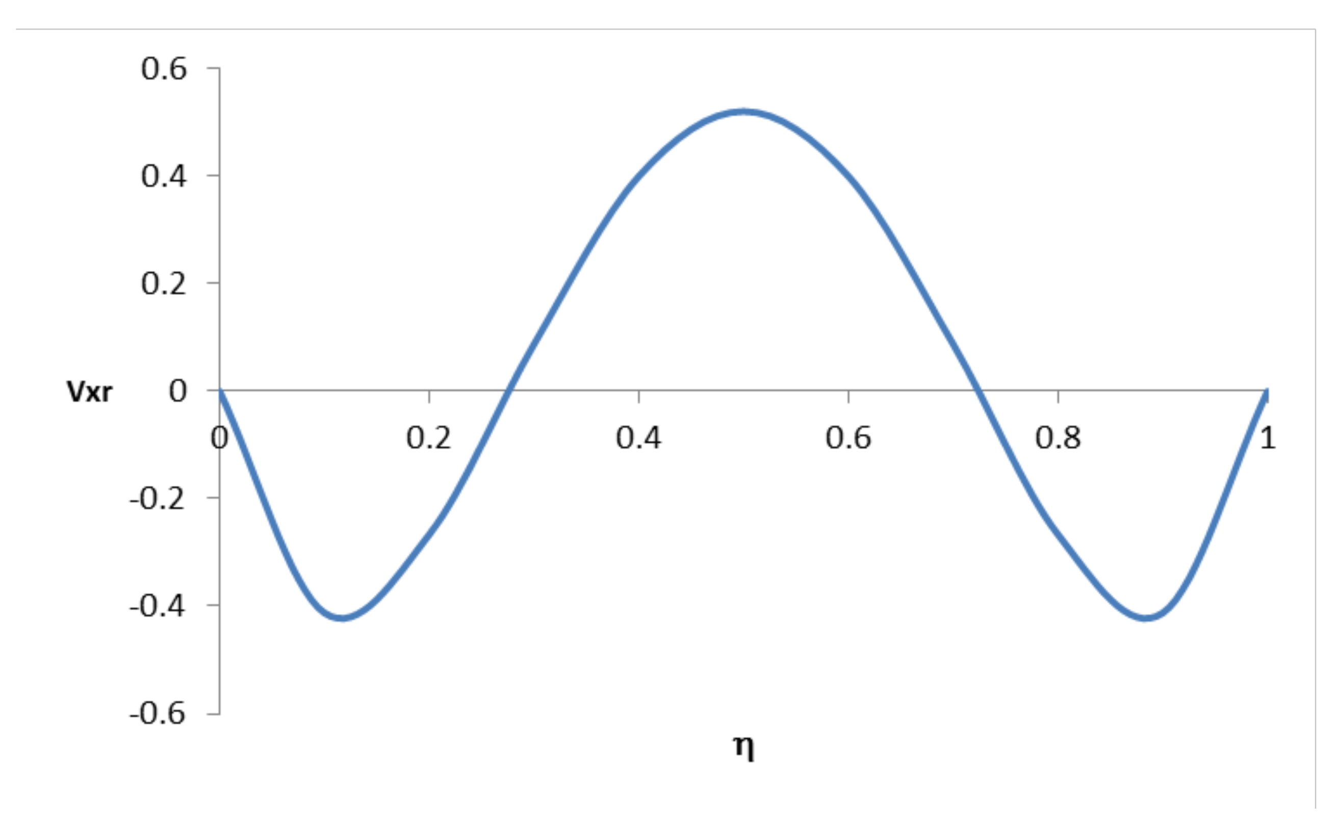
5.1.2. Case 1: Applied to the Hydrodynamic Regime

Based on the heat transfer analysis, $F(R=1,Nu)=1$, the general solution for the “reduced” velocity profile is shown below:

$$V_{xr}(\eta )\equiv \frac{V_x(\eta )}{{\Phi }^{2}Gr\sin (\alpha )}=-\frac{1}{24}(\eta -{\eta }^4)+\frac{1}{12}(\eta -{\eta }^3)+\frac{1}{20}(\eta -{\eta }^2)$$

(55)

It is clear that based on Equation (55), the reduced hydrodynamic velocity profile is independent of Nu. Figure 3 shows the velocity diagram for this case, and it clearly shows the typical flow situation with two (equal) symmetrical zones of decreasing velocity located near the capillary walls and one central zone of ascending velocity. The figure illustrates a situation for which the system cools by having walls at $\eta =0$ and $\eta =1$ at lower temperatures than the center of the capillary domain.

5.2. Case 2: Adiabatic Case for the Capillary Wall Located at $\eta =1$

This case is identified for those values of R where its limit goes to zero. Case 2 applied to the heat transfer and hydrodynamic regimes are shown below.

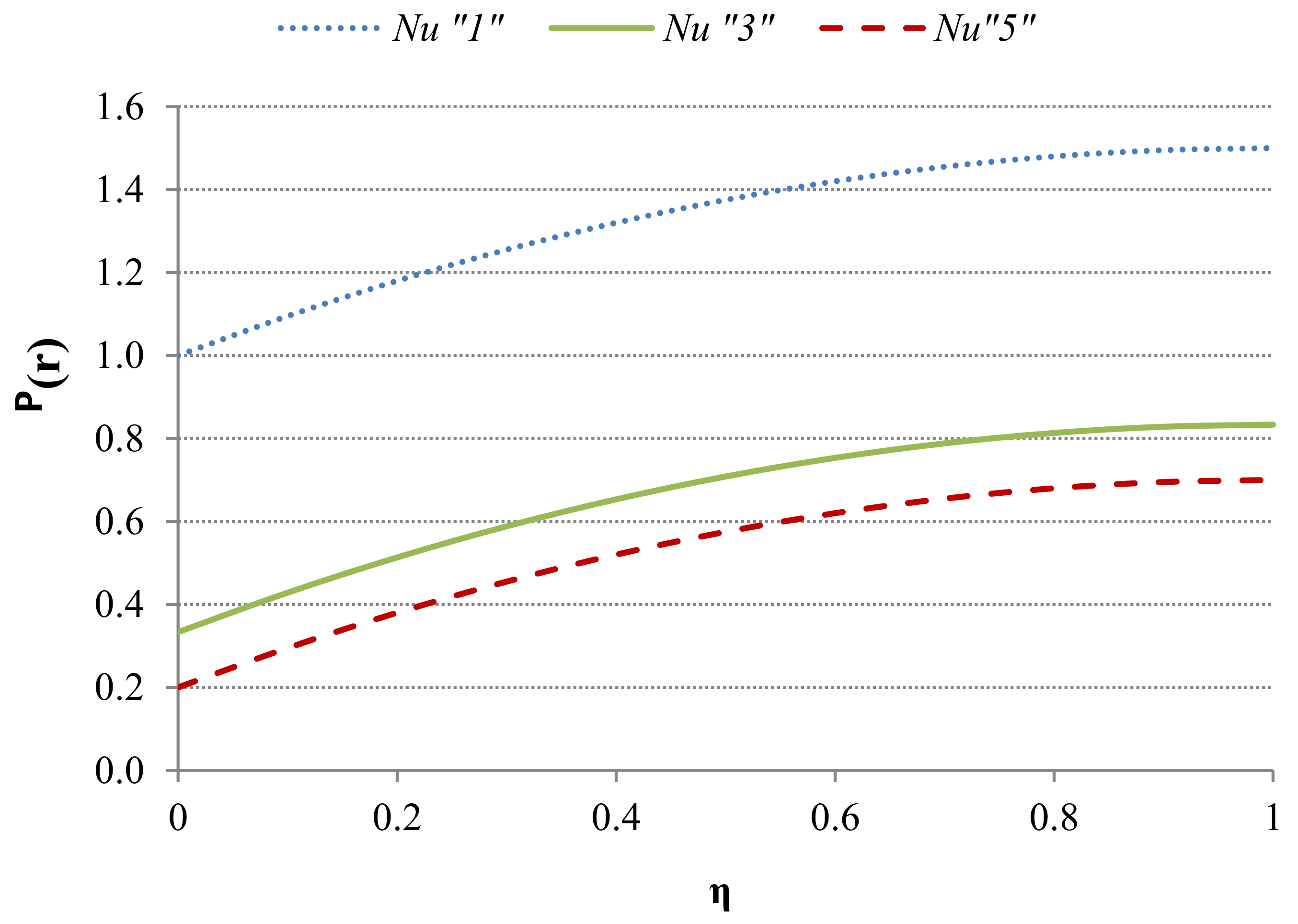
5.2.1. Case 2: Applied to the Heat Transfer Regime

Based on the definition of R, clearly, the temperature gradient at the position $\eta =1$ is zero and, as in the previous case, by using values shown in Table 2 for the R and $F(R,Nu)$, one can conclude by using Equation (22) that the reduced temperature profile is given by (19):

$${\theta }_A^r(\eta )\equiv \frac{\Theta (\eta )}{{\Phi }^2}=-\frac{{\eta }^2}{2}+\eta +\frac{1}{Nu}$$

(56)

This equation is independent of the value of ${\Phi }^2$, as in the symmetrical case, and also has a dependence on the Nusselt number only. In this case, it can be seen that the adiabatic condition is located at η = 1. Therefore, the highest temperature for the case $R=0$ is on the wall located at $\eta =1$; however, these values depend on the Nusselt number (Figure 4). As before, there is a special case for those extremely high values of the Nu number, i.e., $Nu\to \infty$, which leads to:

$${}_{Nu}{\underrightarrow{\lim }}_{\infty }{\theta }_A^r(\eta )\equiv {({\theta }_A^r)}_{\infty }=-\frac{{\eta }^2}{2}+\eta =\eta (1-\frac{\eta }{2})$$

(57)

This function has a maximum value, i.e., ${\left({\theta }_A^r\right)}_{\infty (\eta =1)}=0.5$, at the position $\eta =1$ (the position of one of the capillary walls). The “lowest” temperature, i.e., ${\left({\theta }_A^r\right)}_{\infty (\eta =0)}=0$ of the reduced variable is located at the other wall of the capillary, i.e., $\eta =0$. The function has the other zero located at $\eta =2$, outside the domain of the capillary of Figure 1. Different values of the function of the reduced temperature variable for different values of the Nu numbers are presented in Figure 4.

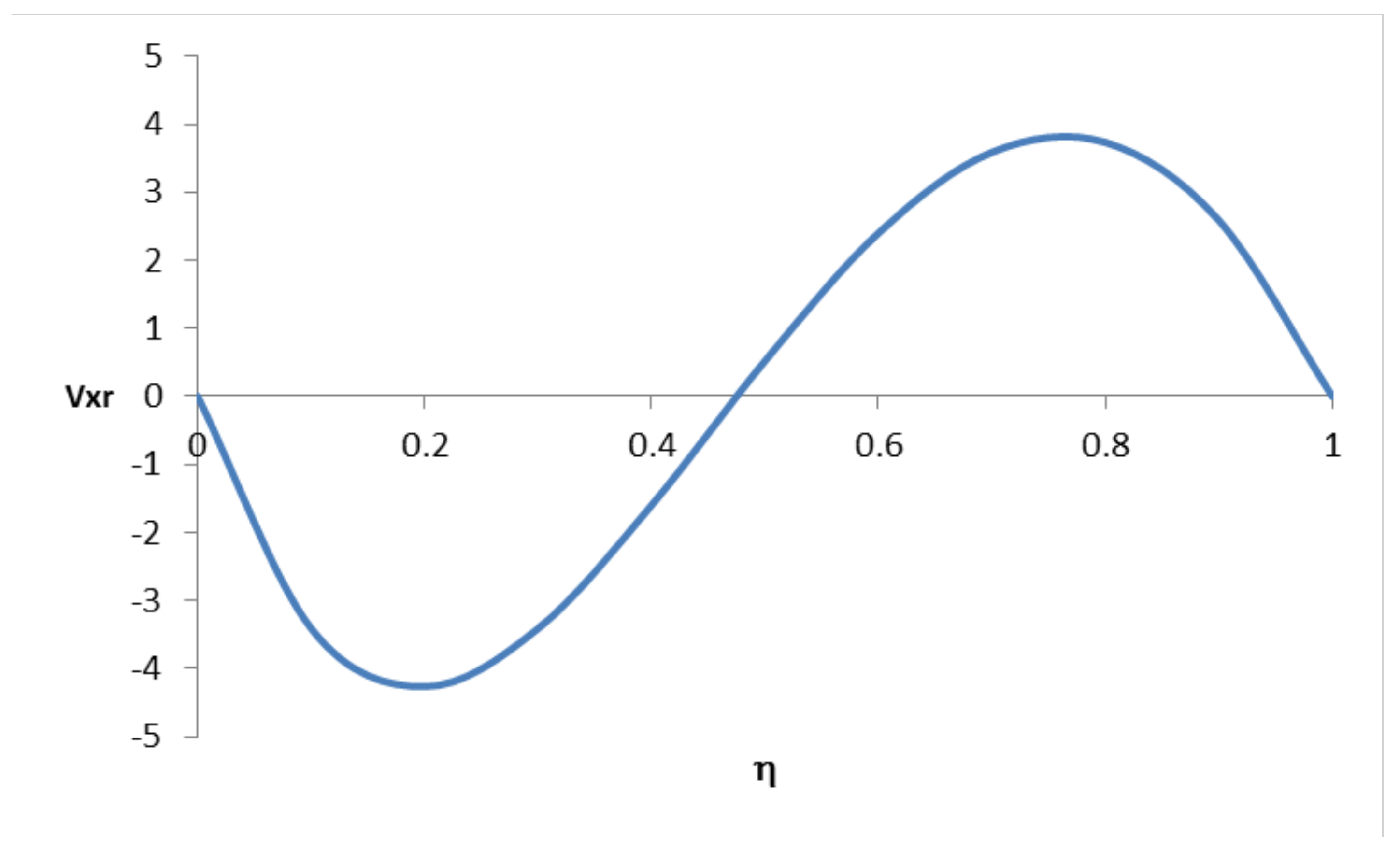
5.2.2. Case 2: Applied to the Hydrodynamic Regime

Based on the definition of factor F, F(R = 0, Nu) = 2 and applying this definition into Equation (52), the following equation is obtained for the hydrodynamic velocity profile:

$$V_{xr}(\eta )\equiv \frac{V_x(\eta )}{{\Phi }^{2}Gr\sin (\alpha )}=-\frac{1}{24}(\eta -{\eta }^4)+\frac{1}{6}(\eta -{\eta }^3)+\frac{7}{40}(\eta -{\eta }^2)$$

(58)

This reduced hydrodynamic velocity profile is independent of the Nusselt number. As indicated above the adiabatic condition is localized at the position $\eta =1$, i.e., the higher value of velocity is located at this position ($\eta =1$) since the temperature takes the maximum value at this position (see Figure 4).

Figure 5 shows that the velocity has ascending values closer to position of the wall at $\eta =1$, due to the fact that at this position the capillary wall has the higher temperature (adiabatic wall). By observing the wall at the position $\eta =0$, it is observed that there is a downward velocity caused by lower temperatures with respect to the wall located at position $\eta =1$. Also, the symmetrical situation described in Figure 3, has been replaced by a “non-symmetrical” one as shown in Figure 5.

5.3. Case 3: Well Mixed Case at the Wall Located at $\eta =1$

This case is identified for values of R → ∞ Case 3 applied to the heat transfer and hydrodynamic regimes are shown below.

5.3.1. Case 3: Applied to the Heat Transfer Regime

When R tends to infinity, we have the following situation:

$${}_R{\underrightarrow{\lim }}_{\infty }\frac{{\Theta }^{\prime }(1)}{R}=0$$

(59)

This indicates, based on the corresponding boundary condition, ($\Theta (1)=0$), that the system has reached a state of well-mixed (WM) condition at this wall position; as the Nusselt number is arbitrary, and we have $\Theta (1)=0$. This implies that the temperature is equal to the room or ambient temperature and that the system has excellent heat transfer conditions at this position. As in previous cases, we calculated the value of $F(R\to \infty ,Nu)$, which implies (see also Table 2) that:

$${}_R{\underrightarrow{\lim }}_{\infty }F(R,Nu)=\frac{Nu}{1+Nu}$$

(60)

By inserting this value into Equation (22), one can conclude that the reduced temperature is given by:

$${\theta }_{MP}^r(\eta )=\frac{\Theta (\eta )}{{\Phi }^2}=-\frac{{\eta }^2}{2}+\frac{Nu\eta }{2(1+Nu)}+\frac{1}{2(1+Nu)}$$

(61)

Clearly, it is only a parametric function of the Nusselt number. For the special case of Nu tending to very large values, the reduced temperature reaches the following function (this function is the same as for the symmetrical case of $R=1$ when the value of the Nu reaches extremely high values).

$${\left({\theta }_{WM}^r\right)}_{\infty }(\eta )=\frac{(1-\eta )\eta }{2}$$

(62)

which indicates zero values (for the reduced temperature) for both $\eta =0$ and $\eta =1$ with its maximum (0.125) located at $\eta =\frac{1}{2}$. Values of the reduced temperature for other values of Nu are illustrated in Figure 6.

5.3.2. Case 3: Applied to the Hydrodynamic Regime

By using the F factor definition: $F(R\to \infty ,Nu)=\frac{Nu}{1+Nu}$, and inserting it into Equation (52), the following equation is obtained for the hydrodynamic velocity profile:

$$V_{xr}(\eta )\equiv \frac{V_x(\eta )}{{\Phi }^{2}Gr\sin (\alpha )}=-\frac{1}{24}(\eta -{\eta }^4)+\frac{1}{12}(\frac{Nu}{(1+Nu)})(\eta -{\eta }^3)+[\frac{3}{40}-\frac{1}{8}(\frac{Nu}{(1+Nu)})](\eta -{\eta }^2)$$

(63)

Contrary to previous cases, the reduced velocity profile is independent of Nu only for very large values. Figure 7 shows illustrations with three different values of the Nusselt number (Nu = 5, Nu = 15, and Nu = 50). In general, Figure 7 shows the opposite situation to that described in Figure 5. Clearly, as the temperature values are reversed, it is observed in Figure 7 that the ascending velocity values are located at position $\eta =0$ while the descending velocity values are located at position $\eta =1$. For the values of Nu = 15 and Nu = 50, the velocity values (near the wall at $\eta =0$) show an “inversion” in the direction of the flow. This inversion, however, is not observed at the position of the wall located at $\eta =1$. Also, as the values of the Nu number increase, the position of the maximum velocity moves toward the center of the capillary and away from the wall located at $\eta =0$. The minimum velocity (located near the wall at $\eta =1$) moves toward the wall. In general, the increase in the values of the Nu numbers moves the hydrodynamic velocity profiles toward a more symmetrical shape with respect to the center position of the capillary.

5.4. Case 4: Favorable Heat Transfer at the Wall Located at $\eta =1$ When R > 1

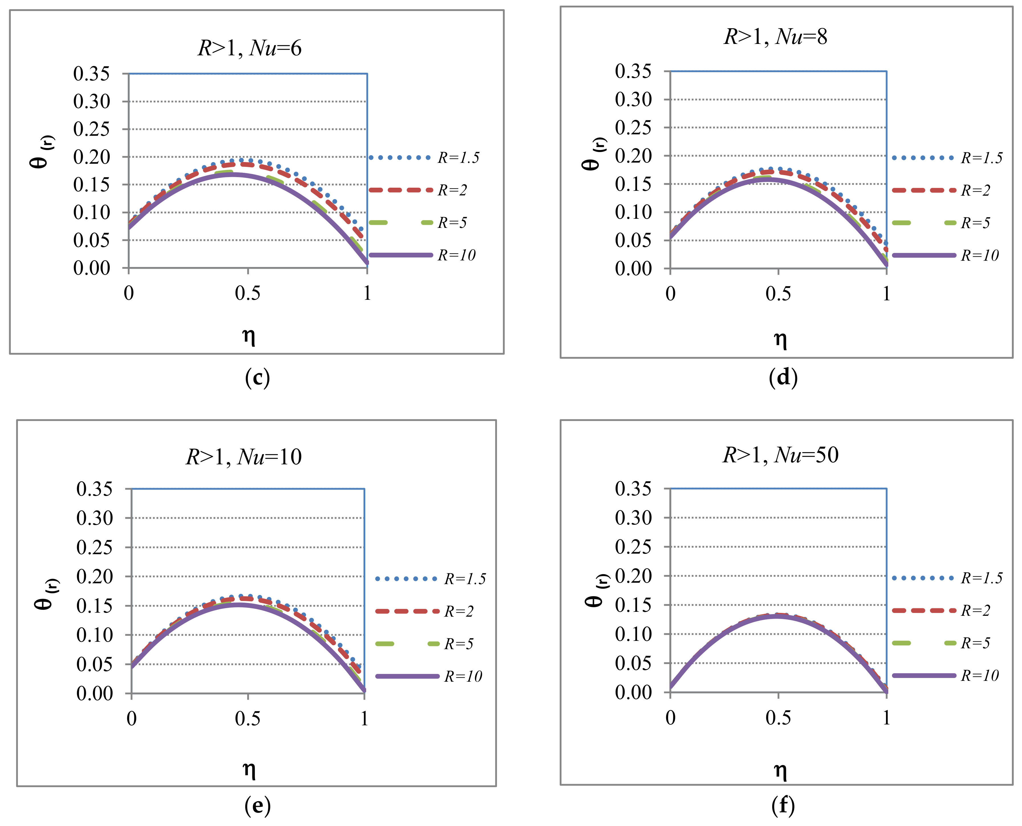
5.4.1. Case 4: Applied to the Heat Transfer Regime

For this case, the rate of heat transfer at the position $\eta =0$ is less than the rate located at position $\eta =1$. The reduced temperature for this general case is given by Equation (22). A numerical illustration is presented in Figure 8 for different values for R (3/2, 2, 5, and 10) and different values for Nu (2, 4, 6, 8, 10, and 50). The important role of the Nusselt number is clearly seen. For example, for the case of Nu = 50 the plots show the significant effect of “collapsing” the plots towards the limiting cases studied in the previous analysis.

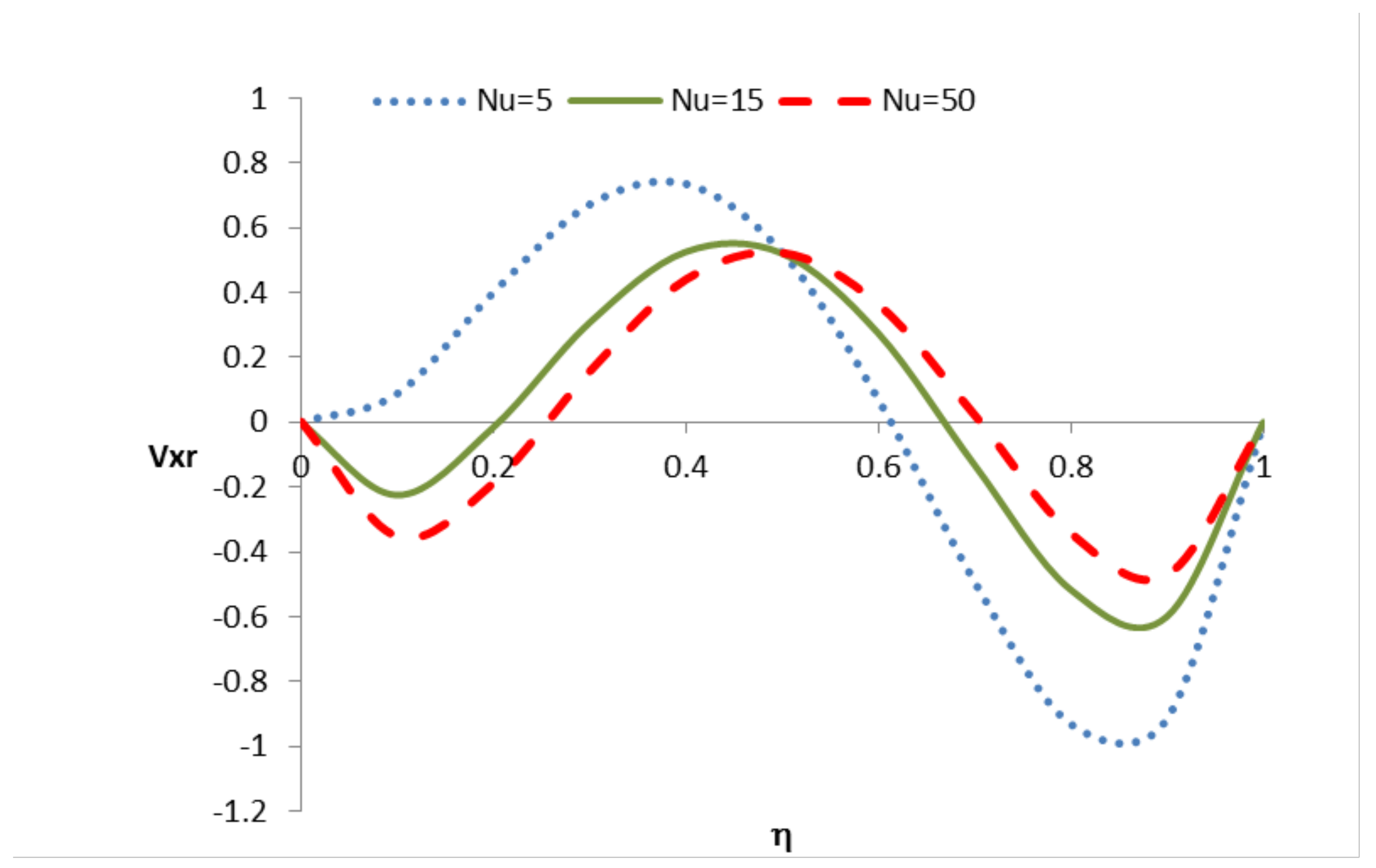
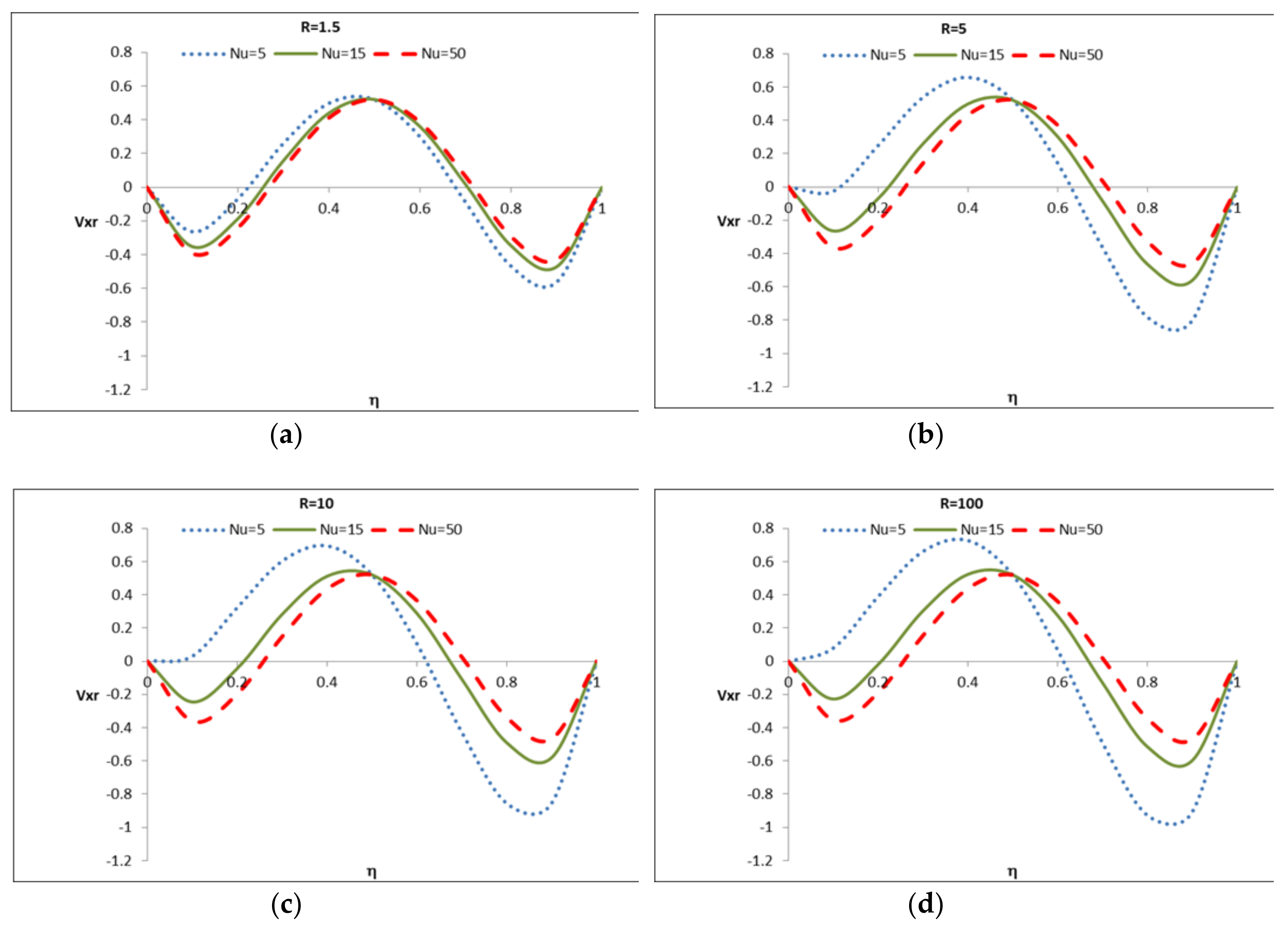
5.4.2. Case 4: Applied to the Hydrodynamic Regime

Figure 9 shows four different cases for the values of the R parameter (R = 1.5; R = 5, R = 10, and R = 100). Each one of the cases is studied (parametrically) with three different values of the Nu number (Nu = 5, Nu = 15, and Nu = 50). For values of the parameter R close to 1 (see, for example R = 1.5), the hydrodynamic velocity profile looks similar to that of the symmetrical case (Case 1, R = 1, see Figure 3). For larger values of the R number (see R = 100), the shape of the hydrodynamic velocity profile looks more like that of Case 3 (the well-mixed condition case). In general, the R values show a “commanding control” for the shape of the hydrodynamic velocity profiles. The Nu number plays a “calibrating role” for the different cases and affects the position of both the maximum and minimum velocity values.

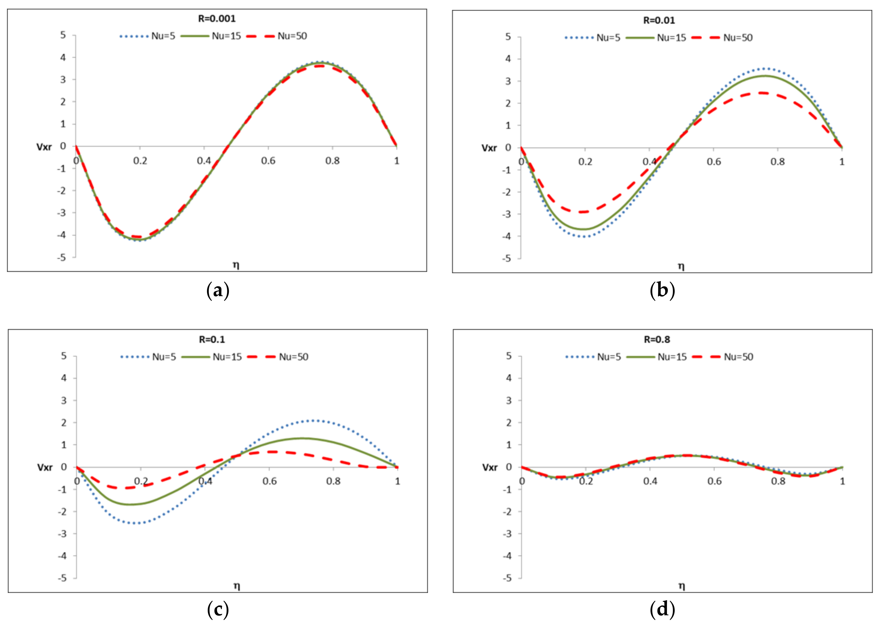
5.5. Case 5: Unfavorable Heat Transfer at the Wall Located at $\eta =1$, (R < 1)

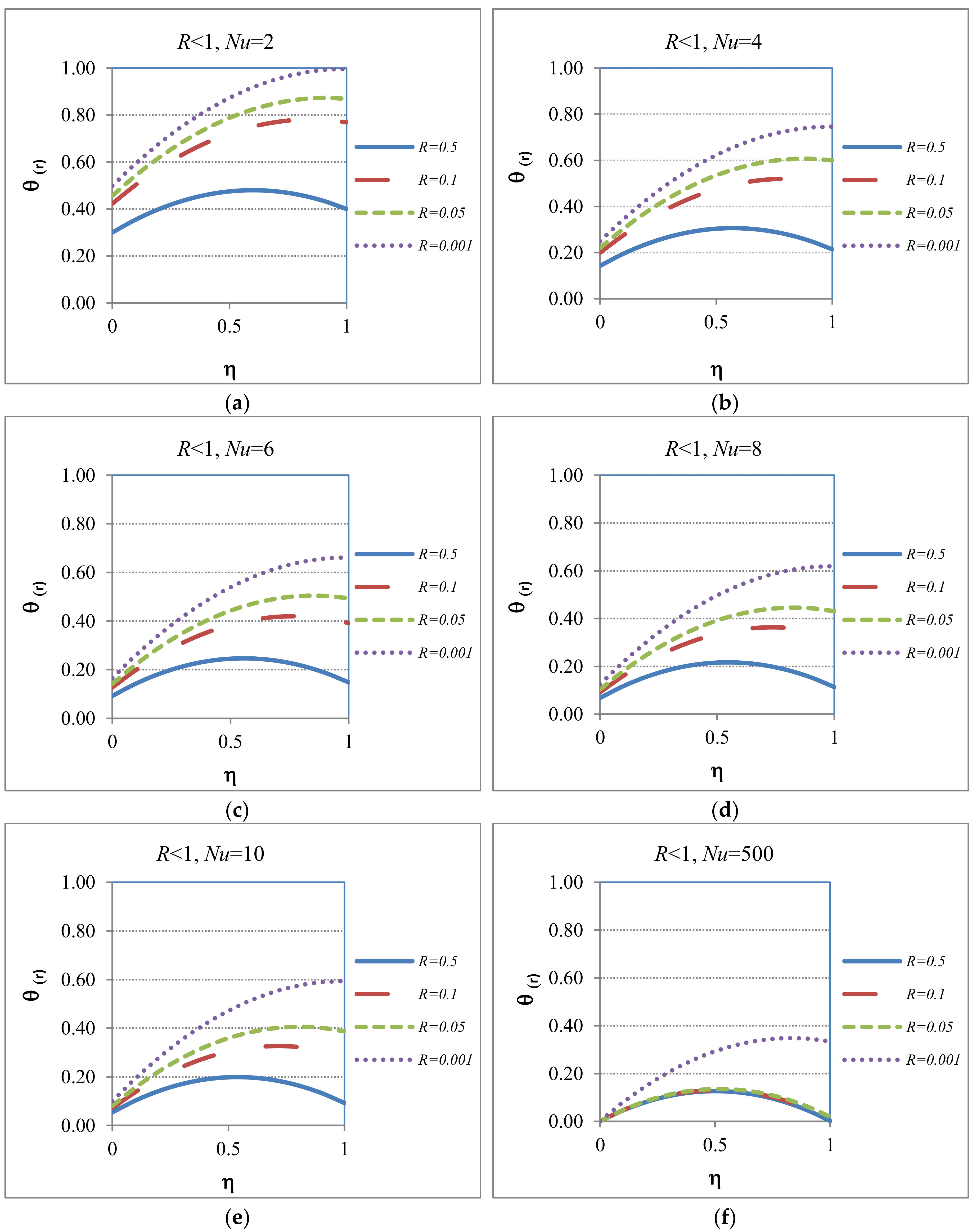
5.5.1. Case 5: Applied to the Heat Transfer Regime

In this case, the same general solution given by Equation (22) is valid, but now R values are less than one. This is the case of heat transfer, for which the rate of heat transfer at the position $\eta =0$ is greater than the heat transfer located at the position $\eta =1$. In this general scenario, different values of R (0.001, 0.1, 0.05, and 0.5), and different values of Nu (2, 4, 6, 8, 10, and 500) were selected to illustrate the behavior of the system (see Figure 10). The general qualitative shapes of the plots look similar to those illustrated in Figure 8; however, both R and Nu control the behavior of the shape of the plots. For example, for Nu = 500, very small values of R are more independent of the “collapsing effect” due to the Nu values. This particular effect will require values of the Nu number in the order of 10,000 [19] to join the other curves.

5.5.2. Case 5: Applied to the Hydrodynamic Regime

Case 5 is the other general case where the velocity follows the unfavorable heat transfer rate for the wall located at position η = 1. The R values for this case less than one. Since the R values cannot be negative, the actual range of values for R is within 0 < R < 1. Figure 11 shows hydrodynamic velocity profiles for four different values of the parameter R (R = 0.001, R = 0.01, R = 0.1, and R = 0.8) within this feasibility range. Each case is studied for three values of the Nusselt number (Nu = 5, Nu = 15, and Nu = 50). From the different cases, one can observe that for the lowest values studied (R = 0.001), the shapes of the velocity profiles look like those of Case 2 (the adiabatic case for the wall at position $\eta =1$, see Figure 5); however, for those values closer to R = 1 (R = 0.8) the shapes of the velocity profiles look like Case 1 (the symmetrical case, Case 1, see Figure 3). As in Figure 9, the one can observe a very controlling effect of the parameter R while, again, the Nu number plays more a “calibrating” effect for the different cases of R values. Cases of R = 0.01 and R = 0.1 seem to be the ones where the Nu number show a more impactful effect (on the shape if the velocity profile) compared to those of R = 0.001 and R = 0.5.

6. Average (Mean) Temperature Analysis of the Capillary

To complete the description of the capillary system, it is also important to consider the relationship between the parametric functions A and B resulting from the total mass conservation, which control the average (or mean) temperature of the system $\overline{\Theta }$; this equation is given by:

$$\overline{\Theta }=\frac{3{\Phi }^2}{10}-\frac{{\Phi }^2}{2}F(R,Nu)+\frac{{\Phi }^2}{Nu}F(R,Nu)$$

(64)

This non-dimensional temperature value $\overline{\Theta }$ is a function of parameters that controls the behavior of the heat transfer system under all conditions assumed for the analysis presented in this contribution, ${\Phi }^2$ and F(R, Nu) Please remember that the factor F(R, Nu) includes R and Nu as parameters.

The reduced mean temperature may be defined as ${\overline{\Theta }}_r=\frac{\Theta }{{\Phi }^2}$, and by using the Equation (64), this definition leads to:

$${\overline{\Theta }}_r=\frac{3}{10}-\frac{1}{2}F(R,Nu)+\frac{1}{Nu}F(R,Nu)$$

(65)

Or, alternatively:

$${\overline{\Theta }}_r=\frac{3}{10}+F(R,Nu)(\frac{Nu-2}{2Nu})$$

(66)

This equation allows a characterization of the different cases; therefore, the behavior of the system can be now completely characterized for both the heat transfer and hydrodynamic aspects. Also, one can obtain the value of the reduced mean temperature $\overline{\Theta }$ for limited cases. For example:

(a)

Symmetrical Case: R = 1, F(R = 1, Nu) = 1, gives:

$${\overline{\Theta }}_r^S=\frac{3}{10}+(\frac{Nu-2}{2Nu})$$

(67)

(b)

Adiabatic Case for the Wall located at $\eta =1$. For this case $R=0$,$F(R=0,Nu)=2$ and it leads to:

$${\overline{\Theta }}_r^A=\frac{3}{10}+[\frac{Nu-2}{Nu}]$$

(68)

(c)

Well-Mixed Case for the Wall Located at $\eta =1$. For this case ($R\to \infty$), we have, $F(R\to \infty ,Nu)=\frac{Nu}{1+Nu}$, and it leads to:

$${\overline{\Theta }}_r^{WM}=\frac{3}{10}+\frac{(Nu-2)}{2(1+Nu)}$$

(69)

Regarding the general case, R < 1 and R > 1, these can be obtained directly from Equation (68).

7. Conclusions

In the present work, heat transfer and hydrodynamic aspects of the effect of Joule heating for cases where the contaminated soil may show non-uniform conditions are reported. This information is useful for understanding the effect of both the temperature and hydrodynamics on the design of cleaning strategies when the soil shows non-uniform properties.

Interestingly, two parameters, i.e., the R factor (ratio between the Nusselt numbers at both walls of the capillary) and F(R, Nu). (a function associated with Nusselt number and the non-dimensional ratio R) are useful for identifying different situations or “regimes” in the flow of the system. These parameters control the behavior of the system in both aspects: thermal and the hydrodynamics.

As indicated above, by using the ratio of Nusselt numbers located at both capillary boundaries, R, different heat transfer regimes have been defined. For example, the value of R = 0 indicates the adiabatic condition at one boundary, R = 1, the symmetric condition, and R taking a very large value (∞) implies a well-mixed condition at a given capillary boundary. The definition of R is complemented by the factor $F\left(R, Nu\right)$ that coincidentally takes the values of 1, 2 and $Nu/\left(1+Nu\right)$ as “symmetric”, “adiabatic” and “well-mixed” boundaries, respectively, for the values of R previously indicated. In addition, two more R value ranges are identified, i.e., R > 1, named the favorable heat transfer case at the position of the capillary wall located at $\eta =1$ and R < 1, as the unfavorable heat transfer case at the same location of the capillary wall. All of these situations develop very distinct heat transfer and hydrodynamic behaviors with specific types of temperature and velocity profiles. Practical implications need to be assessed by experiments; however, the results presented here are helpful to guide these applications and, therefore, avoid the development of adverse conditions such as flow reversal [14].

In summary, the present work shows a clear picture of what happens with the temperature and hydrodynamics in different cases along with potential cleaning conditions. Also, the potential significant changes that could develop in capillary domains (in the soil) when non-uniform conditions are present in the soil matrix are also shown. Future work includes extending this analysis to soils with electrical charges in their matrix by incorporating electroosmotic effects.

References

1. Reddy, K.R.; Cameselle, C. Electrochemical Remediation Technologies for Polluted Soils, Sediments and Groundwater; John Wiley & Sons: New York, NY, USA, 2009. [Google Scholar]
2. Iyer, R. Electrokinetic Remediation. Particul. Sci. Technol. 2001, 19, 219–228. [Google Scholar] [CrossRef]
3. Wada, S.I.; Umegaki, Y. Major ion and electrical potential distribution in soil under electrokinetic remediation. Environ. Sci. Technol. 2001, 35, 2151–2155. [Google Scholar] [CrossRef] [PubMed]
4. Suèr, P.; Nilsson-Påledal, S.; Norrman, J. LCA for site remediation: A literature review. Soil Sediment Contam. 2004, 13, 415–425. [Google Scholar] [CrossRef]
5. Romantschuk, M.; Sarand, I.; Petänen, T.; Peltola, R.; Jonsson-Vihanne, M.J.; Koivula, T.; Yrjälä, K.; Haahtela, K. Means to improve the effect of in situ bioremediation of contaminated soil: An overview of novel approaches. Environ. Pollut. 2000, 107, 179–185. [Google Scholar] [CrossRef]
6. Mulligan, C.N.; Yong, R.N.; Gibbs, B.F. An evaluation of technologies for the heavy metal remediation of dredged sediments. J. Hazard. Mater. 2001, 85, 145–163. [Google Scholar] [CrossRef]
7. Pavel, L.V.; Gavrilescu, M. Overview of ex situ decontamination techniques for soil cleanup. Environ. Eng. Manag. J. 2008, 7, 815–834. [Google Scholar]
8. Dellisanti, F.; Rossi, P.L.; Valdrè, G. Mineralogical and chemical characterization of Joule heated soil contaminated by ceramics industry sludge with high Pb contents. Int. J. Miner. Process. 2007, 83, 89–98. [Google Scholar] [CrossRef]
9. Dellisanti, F.; Rossi, P.L.; Valdrè, G. In-field remediation of tons of heavy metal-rich waste by Joule heating vitrification. Int. J. Miner. Process. 2009, 93, 239–245. [Google Scholar] [CrossRef]
10. Dellisanti, F.; Rossi, P.L.; Valdrè, G. Remediation of asbestos containing materials by Joule heating vitrification performed in a pre-pilot apparatus. Int. J. Miner. Process. 2009, 91, 61–67. [Google Scholar] [CrossRef]
11. Boland, M.; Arce, P.; Erdmann, E. Free convection flows in fibrous or porous media: A solution for the case of homogeneous heat sources. Int. Commun. Heat Mass Transf. 2000, 27, 745–754. [Google Scholar] [CrossRef]
12. Oyanader, M.A.; Arce, P.E. Role of joule heating on the hydrodynamic boundary layer with rectangular electrodes: Numerical approach. Lat. Am. Appl. Res. 2008, 38, 147–154. [Google Scholar]
13. Oyanader, M.A.; Arce, P.E.; Bolden, J.D. Role of joule heating in electro-assisted processes: A boundary layer approach for rectangular electrodes. Int. J. Chem. Reactor Eng. 2013, 11, 815–823. [Google Scholar] [CrossRef]
14. Oyanader, M.A.; Arce, P.; Dzurik, A. Avoiding pitfalls in electrokinetic remediation: Robust design and operation criteria based on first principles for maximizing performance in a rectangular geometry. Electrophoresis 2003, 24, 3457–3466. [Google Scholar] [CrossRef] [PubMed]
15. Chakraborty, R.; Dey, R.; Chakraborty, S. Thermal characteristics of electromagnetohydrodynamic flows in narrow channels with viscous dissipation and Joule heating under constant wall heat flux. Int. Commun. Heat Mass Transf. 2013, 67, 1151–1162. [Google Scholar] [CrossRef]
16. Tijaro-Rojas, R. Role of Micro and Macro-Heterogeneities in Electro-kinetic Soil Cleaning: An Area-Averaging Approach with Dynamic Simulations. Ph.D. Thesis, Tennessee Technological University, Cookeville, TN, USA, 2015. [Google Scholar]
17. Tíjaro-Rojas, R.; Arce-Trigatti, A.; Cupp, J.; Pascal, J.; Arce, P.E. A Systematic and Integrative Sequence Approach (SISA) for mastery learning: Anchoring Bloom’s Revised Taxonomy to student learning. Educ. Chem. Eng. 2016, 17, 31–43. [Google Scholar] [CrossRef]
18. Batchelor, G.K. Heat transfer by free convection across a closed cavity between vertical boundaries at different temperatures. Q. Appl. Math. 1954, 12, 209–233. [Google Scholar] [CrossRef] [Green Version]
19. Torres, C. Limpieza de Suelos Usando Tecnicas Electrocineticas: Rol del Número de Nusselt en Modelos Capilares Rectangulares con Calentamiento joule. Master’s Thesis, Universidad Catolica del Norte, Antofagasta, Chile, July 2011. [Google Scholar]
20. Dullien, F.A.; Dong, M.; Dai, L.; Li, D. Immiscible Displacement in the Interacting Capillary Bundle Model Part I. Development of Interacting Capillary Bundle Model Title. Transp. Porous Media 2005, 59, 1–18. [Google Scholar] [CrossRef]
21. Bird, R.; Stewart, W.; Lightfoot, E. Transport Phenomena; John Wiley & Sons: New York, NY, USA, 2002. [Google Scholar]
22. Halliday, D.; Resnick, R.; Walker, J. Fundamentals of Physics Extended, 10th ed.; Wiley: New York, NY, USA, 2013. [Google Scholar]
23. Pascal, J.; Tíjaro-Rojas, R.; Oyanader, M.A.; Arce, P.E. The acquisition and transfer of knowledge of electrokinetic-hydrodynamics (EKHD) fundamentals: An introductory graduate-level course. Eur. J. Eng. Educ. 2017, 42, 493–512. [Google Scholar] [CrossRef]
24. Gebhart, B.; Jaluria, Y.; Mahajan, R.L.; Sammakia, B. Buoyance-Induced Flows and Transport; Hemisphere Publishing Corporation: New York, NY, USA, 1988. [Google Scholar]
Figure 1. A sketch of the capillary domain in rectangular coordinates showing key dimensions and coordinate system, showing the length (L), width (H), depth (W) and an inclination of an angle α (0–90°) with respect to the orientation of gravity “g”.
Environments 05 00092 g001
Figure 2. Behavior of the reduced non-dimensional temperature profiles vs. the Nusselt number: symmetric case (R = 1).
Environments 05 00092 g002
Figure 3. Reduced Non-dimensional Velocity Profile for Symmetrical Case (R = 1). (Velocity values have been scaled ×103).
Environments 05 00092 g003
Figure 4. Behavior of the non-dimensional reduced temperature profiles vs. the Nusselt number: Adiabatic Case (R = 0).
Environments 05 00092 g004
Figure 5. Reduced non-dimensional velocity profile for adiabatic Case ( R = 0 ). (Velocity values have been scaled ×100).
Environments 05 00092 g005
Figure 6. Behavior of the reduced non-dimensional temperature profiles vs. the Nusselt number: Well-Mixed Case (R → ∞).
Environments 05 00092 g006
Figure 7. Reduced Non-dimensional Velocity Profile for Well-Mixed Case (R → ∞) and with different values for the Nu numbers (Velocity values have been scaled ×103).
Environments 05 00092 g007
Figure 8. Behavior of the non-dimensional reduced temperature profiles vs. the Nusselt Number: Heat Transfer Favorable Case at η = 1 , (R > 1), for different values for R (3/2, 2, 5, and 10). (af), correspond to the different values for Nu of 2, 4, 6, 8, 10 and 50, respectively.
Environments 05 00092 g008aEnvironments 05 00092 g008b
Figure 9. Reduce non-dimensional Velocity Profile: Heat Transfer Favorable Case for R > 1 and Nu = 5, 15, and 50 (Velocity values have been scaled ×103). (ad), correspond to the different values for R of 1.5, 5, 10 and 100, respectively.
Environments 05 00092 g009
Figure 10. Behavior of the non-dimensional reduced temperature profiles vs. the Nusselt number at values of R (0.001, 0.1, 0.05, and 0.5): Heat Transfer Unfavorable Case at η = 1 , (R < 1). (af), correspond to the different values for Nu of 2, 4, 6, 8, 10 and 500, respectively.
Environments 05 00092 g010
Figure 11. Non-dimensional Reduced Velocity Profile: Heat Transfer Unfavorable Case for R < 1 and Nu = 5, 15, 50 (Velocity values have been scaled ×103). (ad), correspond to the different values for R of 0.001, 0.01, 0.1 and 0.8, respectively.
Environments 05 00092 g011