Article

Land Use/Land Cover Change Detection and Urban Sprawl Analysis in the Mount Makiling Forest Reserve Watersheds and Buffer Zone, Philippines

1
Geospatial Integration Division-Resource Data Analysis Branch, National Mapping and Resource Information Authority, Taguig City 1634, Philippines
2
Environmental Science Department, Eastern Samar State University-Salcedo Campus, Salcedo 6807, Eastern Samar, Philippines
3
College of Agriculture, Southern Luzon State University, Lucban 4328, Quezon, Philippines
4
Institute of Computer Science, College of Arts and Sciences, University of the Philippines Los Baños, Los Baños 4031, Laguna, Philippines
5
Makiling Center for Mountain Ecosystems, College of Forestry and Natural Resources, University of the Philippines Los Baños, Los Baños 4031, Laguna, Philippines
6
Environmental Remote Sensing and Geo-information Laboratory, Institute of Renewable Natural Resources, College of Forestry and Natural Resources, University of the Philippines Los Baños, Los Baños 4031, Laguna, Philippines
*
Author to whom correspondence should be addressed.
Submission received: 21 September 2018 / Revised: 2 November 2018 / Accepted: 18 November 2018 / Published: 24 January 2019
(This article belongs to the Special Issue Technologies for Sustainable Environmental Systems)

Abstract

:
Ecologically Valuable Areas play an important role in providing ecosystem services, however, human activities such as land conversion and urban sprawl pose pressures and threats to these areas. The study assessed the land use/land cover and urban sprawl in the Mount Makiling Forest Reserve (MMFR) Watersheds and Buffer Zone from 1992 to 2015 using remote sensing and Geographic Information System (GIS). Results showed that the land use/cover within the MMFR buffer zone has changed from 1992 to 2015 with built-up areas increasing by 117% despite Proclamation 1257, s. 1998 which regulates human activities in the zone. Based on the Shannon entropy analysis the land development in the MMFR buffer zone tends to be dispersed and sprawling. However, when the magnitude of change of urban sprawl in the buffer zone from 2002 to 2015 was calculated, a decrease in the entropy value was observed which implies a compacting pattern as the human settlement in the buffer zone increases over time. Proclamation 1257, s. 1998 needs to be strengthened to protect MMFR and its buffer zone from further encroachment and pressure. Moreover, remote sensing and GIS proved to be useful tools for assessing urban sprawl in ecologically valuable areas such as MMFR.

1. Introduction

Ecologically valuable areas (e.g., forest reserve, national parks, and protected areas) [1] within the borders of urban areas provide many ecosystem services for urban [2] and neighboring population. These areas are especially valuable for the protection of biodiversity ([3,4,5]; as cited in [6]). Despite their importance, ecologically valuable areas are threatened with the continuing urbanization [1]. The impacts of urbanization along the fringes of these areas include fragmentation of habitats, loss of rare species, edge effects, the introduction of alien species, degradation of the environment, reduced tourism potential and the loss of ecosystems services vital for the wellbeing and health of urban residents ([1,7,8]; as cited in [9]). According to Mutuga [9], the harmful effects of urbanization is particularly caused by urban sprawl. Urban sprawl is the expansion of human settlement or development outside of an urban city center [10]. As urban areas expand they take up more land and extends further to ecologically valuable areas [9]. A disproportionate increase in the population growth near the boundaries of ecologically valuable areas may threaten their ability to conserve biodiversity [11]. Urbanization near the borders of ecologically valuable areas creates a conflict between biodiversity protection and demands for housing and economic development. These conflicts are more frequent and intensive in areas with a greater number of rare and endangered species and in areas with severe population and development pressures ([12]; as cited in [9]).
In response to these problems, buffer areas have been designed to protect and enhance the conservation value of ecologically valuable areas. However, Rathore [13] notes that most forest buffers have already been reduced to a degraded status due to the massive pressures from adjacent settlements. McDonald, Kareiva, and Forman [14] observed the shrinking distance between protected areas and cities in some parts of the world. Considering these threats and pressures, periodic assessment [15] and monitoring of the urban development are important for conservation [16] and protection of ecologically valuable areas from further degradation, to evaluate natural resources and the effectiveness of management [15] and to make effective and appropriate measures using remote sensing and Geographic Information System (GIS) [16]. Remote sensing is a cost-and-time efficient tool [17] that can be used for monitoring urban expansion [16,18] and the impact of human activities on the landscape [17] of forest reserves, national parks or protected areas. Remote sensing is a science and art of acquiring information about the Earth’s surface and atmosphere using sensors designed to detect electromagnetic radiation either ground-based, aerial or spaceborne platforms [19,20]. It is a reliable source of data, provides spatially consistent coverage of large areas with temporal frequency, and high spatial detail, which is useful for analyzing time-dependent phenomenon such as urban expansion [21,22].
This study assessed the land use/land cover change and urban sprawl in the Mount Makiling Forest Reserve (MMFR) Watersheds and its buffer zone from 1992 to 2015. Shannon’s entropy was calculated to characterize and measure the relative trends in the dispersion or compaction of urban sprawl in the MMFR watersheds and its buffer zone. The magnitude of change of urban sprawl in the watersheds and its buffer zone over time was also analyzed.

2. Materials and Methods
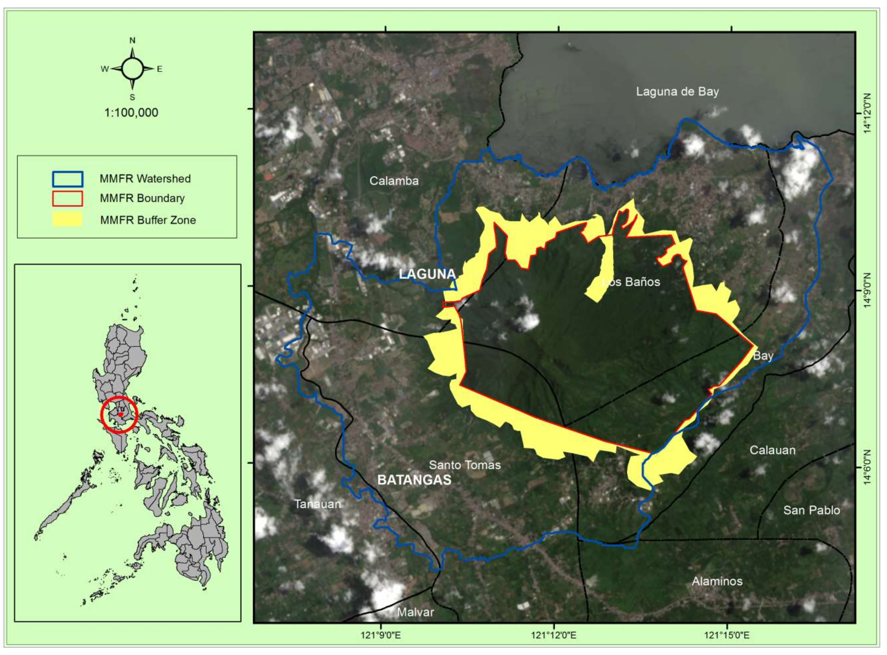
2.1. Study Site

The Mount Makiling Forest Reserve (MMFR) is an important landscape and “training laboratory for the advancement of science and technical knowledge for the conservation and development of forests and associated ecosystems” [23]. Mount Makiling is also an important catchment area for Laguna de Bay [24,25] providing a water supply for industrial, agricultural and residential sectors of the CALABARZON (Cavite, Laguna, Batangas, Rizal, and Quezon) region [26]. MMFR is also classified as a national park ([27]; as cited in [28]) and was declared as the 33rd ASEAN (Association of Southeast Asian Nations) Heritage Park on 3 October 2013 [29]. By virtue of Republic Act 6967 (Section 3), the exclusive control, jurisdiction, and management of MMFR was handed to the University of the Philippines Los Baños (UPLB) [23]. MMFR covers a total land area of 4224 hectares and lies between 14°06′ to 14°15′ north latitude and 121°09′ to 121°16′ east longitude [24]. The forest reserve covers parts of the municipalities of Bay, Calamba City and Los Baños in the province of Laguna, and Santo Tomas in the province of Batangas [30]. There are four watersheds in MMFR and these are the Molawin-Dampalit Watershed, Cambantoc Watershed, Tigbi Watershed and the Greater Sipit Watershed. In this study, they are collectively referred to as MMFR Watersheds.
Proclamation 1257 or “Designating Certain Areas Surrounding the Makiling Forest Reserve as Buffer Zone and Prescribing Guidelines Thereof” institutionalize the coverage of MFFR buffer zone. Accordingly, areas adjacent to the MMFR boundary with 18% slope and above (Figure 1. Map of Mount Makiling Forest Reserve Buffer Zone) forms part of the park’s buffer zone. Proclamation 1257 was passed in 1998 “to guide the local government units (LGUs), entrepreneurs, developers, businessmen, landowners and other interested individuals on the use of the buffer zone surrounding the MMFR. It was also intended to avoid further encroachment on the forest reserve that would create disturbances or damage to the ecology of the area and reconcile socio-economic undertakings and environmental protection on the use of the buffer area to minimize negative off-site effects of land developments therein” [31]. However, despite the Proclamation, MMFR is continually being threatened by the expansion of human settlements, agricultural areas, and urban and industrial zones [24]. The urbanization along the borders of MMFR and the development of residential subdivisions on its lower slopes also adds pressure on the forest reserve [32], which may eventually have tremendous impacts on the communities depending on it [33].
The buffer zone covers portions of the alienable and disposable land of the municipalities of Bay, Los Baños, and Santo Tomas, and the city of Calamba. The population density in these areas averages as more than 1000 individuals per km2 (Table 1. Population, Land Area and Population Density of Areas portions of which are covered by the Mount Makiling Forest Reserve). Among the municipalities, Bay is the smallest in terms of land area with only 42.66 km2. It is a second-class municipality with a population of 62,143 [34]. The municipality of Los Baños is a first-class municipality with a land area of 54.22 km2 and a population of 112,008 [34]. Los Baños is also considered as a Special Science and Nature City of the Philippines [35]. Calamba City is a first-class city and the most populated city in the province of Laguna. Calamba City is the center of commerce and industry in the province and has attracted many job seekers from nearby provinces which have led to a significant increase in its population [36]. The population in Calamba City has increased from 389,377 in 2010 [37] to 454,486 in 2015 [34]. Santo Tomas is also a first-class municipality and one of the oldest towns of Batangas [38]. The municipality has a land area of 95.41 km2 and a population of 179,884 [34].

2.2. Urban Sprawl Detection and Assessment

Various procedures were utilized to assess the urban sprawl in the buffer zone of MMFR, Philippines (Figure 2). These include data acquisition, image preprocessing, classification and analysis, post-processing, accuracy assessment, and Shannon’s entropy calculation.

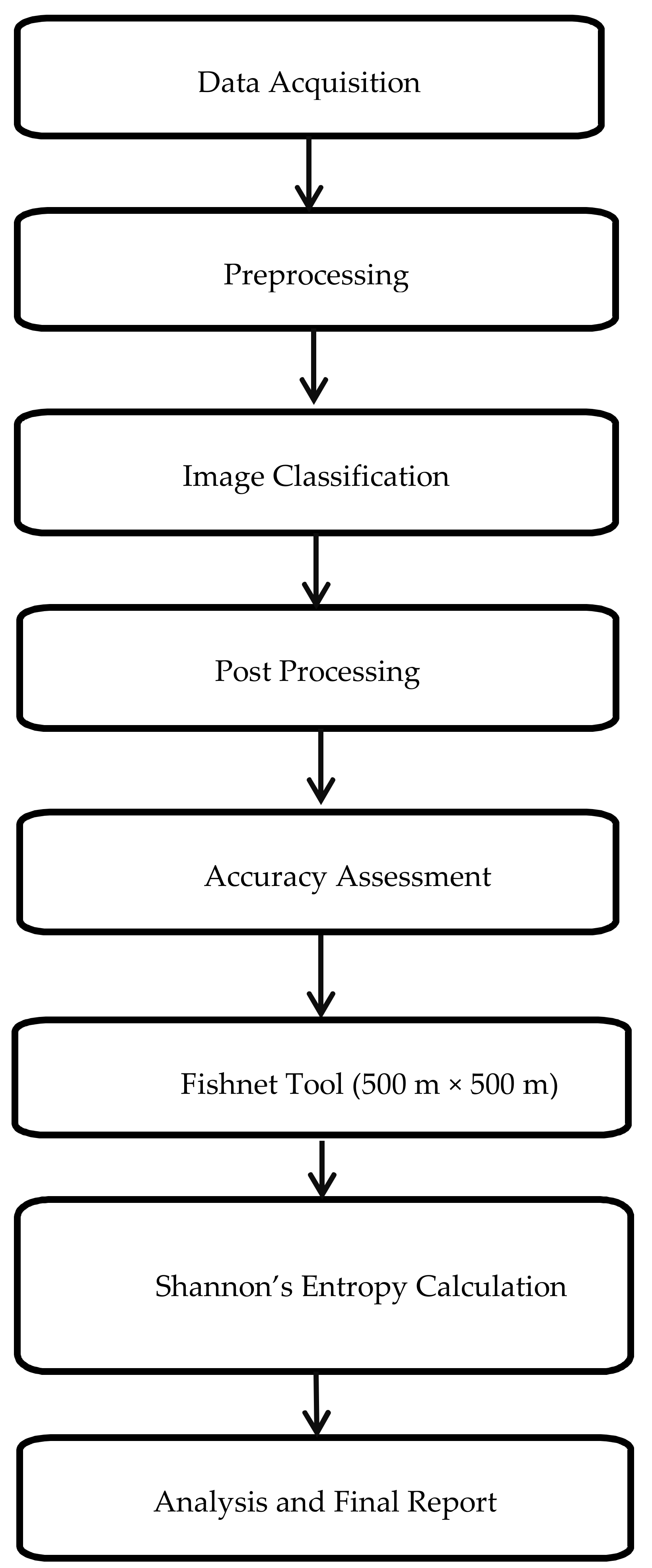
2.2.1. Spatial Data Acquisition

The study utilized information in vector and raster format including those acquired through remote sensing platforms. The different data used in the study are summarized in Table 2. Vector data include the physical boundary of MMFR watersheds, MMFR boundary, and MMFR buffer zone boundary which were requested from Makiling Center for Mountain Ecosystems (MCME) in UPLB. The Landsat satellite images were acquired from 26 January 1992 (Landsat Thematic Mapper (TM)) [40], 4 April 2002 (Landsat 7 Enhanced Thematic Mapper Plus (ETM+)) [41] and 29 July 2015 (Landsat 8 Operational Land Imager/Thermal Infrared Sensor (OLI/TIRS)) [39]. These were downloaded from the USGS Earth Explorer website [39,40,41] in October 2017. The selected images were either cloud-free or present cloud cover of less than 10% to achieve more accurate results of the study. All vector and raster files were projected into Universal Transverse Mercator (UTM) System, Zone 51 North and World Geodetic System (WGS) 84 datum.

2.2.2. Image Preprocessing

Image preprocessing prepares and restores band data by recalculating Digital Number (DN) values and eliminating external and space-borne platforms errors. A standard radiometric calibration was applied to enhance DN values and extract the Top-of-Atmosphere (TOA) reflectance [42] of the satellite images covering the MMFR that were taken at different periods. The preprocessing of the Landsat images was conducted using the ENVI 5.2 software (Exelis Visual Information Solutions, Boulder, CO, USA). Only a subset containing the MMFR boundary was extracted and processed for a more focused analysis and better data handling.
The surface reflectance free from clouds and other atmospheric components was also determined which is vital in many remote sensing applications [19,43]. Pan-sharpening of the Landsat 7 and 8 satellite images was completed using the Gram Schmidt method in the ENVI 5.2 software to maximize the available high-resolution panchromatic band (15-m) by combining it with a low-resolution multispectral image (30-m).

2.2.3. Classification and Analysis

The supervised classification method employs the Maximum Likelihood Classification (MLC) to classify and segment the pre-processed Landsat satellite images. MLC quantitatively analyze remote sensing data [19,44,45,46] by classifying each cell based on the highest probability of being a member and spectral pattern represented in class mean vectors and covariance matrices [46]. For Supervised classification, representative pixels or training data [46] for each land cover classes to be segmented were selected and utilized in the classification algorithm. Ten (10) training points per land cover class were identified and randomly selected from Google Earth [47] online [48,49] for Landsat 8 (Table 3). The land cover classes of these training points were determined using the Food and Agriculture Organization (FAO) land cover classes and description [50]. Likewise, the land cover classes of these training points were identified from Landsat 5 (81 random points), Landsat 7 (104 random points) and Landsat 8 (72 random points) satellite images for change analysis.

2.2.4. Accuracy Assessment

Classification accuracy refers to the extent of correspondence between remotely sensed data and reference data [51]. The generated land cover data from Landsat 8 were assessed through a selection of 30 sampling points [45] per class using the Google Earth [47] online [44,52]. It was assumed that the 2015 classified map accuracy was enough to justify the overall accuracy of the study area in the different periods [53]. The accuracy assessment of the classified images was performed using the ArcGIS 10.5 software (Environmental Systems Research Institute, Redlands, California, CA, USA) and the results were shown in a confusion matrix. The overall accuracy was generated which shows the overall quality of the data by dividing the total correct pixels by the total number of pixels. Kappa coefficient was also used to measure the classification accuracy. Kappa coefficient (K) is a discrete multivariate technique commonly used in accuracy assessment that provides a more unbiased estimate of overall agreement [48,54]. The K interpretation values range from poor to excellent agreement ranging from 0 to 1. The closer the value of K to one (1.0) the more acceptable the classification [48]. The error of commission and omission were also calculated. The error of commission represents pixels or the reliability of the map since it indicates how accurate the maps are to represent what is actually seen on the ground while the error of omission represents pixels that belong to the truth class but fail to be classified into the proper class. User and producer accuracy was also generated using the correct classified pixel per category (row and column) divided by the total pixel per class (row and column).

2.2.5. Classification Post Processing

Final data editing, consolidation, and integration are important procedures to enhance the quality of the final map [44]. The post-classification change detection technique, which detects the nature, rate, and location of changes was used in this study. Vectorization using unsimplified polygons [44,55] of the classified images was executed to generate the total area and land cover change per class in hectare per satellite scene. Final data editing and integration were implemented for doubtful areas (e.g., clouds using secondary data such as land cover maps [56], Google Earth [47] and personal knowledge in the study site). The MMFR landscape patterns were determined based on the post edited final results of the image classification. The overlay analysis e.g., intersection of the final MMFR watersheds’ land cover maps and the MMFR buffer zone was conducted to extract the landcover patterns inside the MMFR buffer zone for 1992, 2002 and 2015.
Using an overlay procedure in GIS, spatial changes in the Land Use/Land Cover (LULC) of the Mount Makiling Forest Reserve watersheds and buffer zone in two phases (i.e., 1992–2002, 2002–2015) were determined. This technique resulted in a cross-tabulation matrix describing the main types of change in the study area. The cross-tabulation obtained was analyzed on a pixel-by-pixel basis and this procedure consequently facilitated the determination of the number of conversions from a particular class to other land use classes and their corresponding area and weight of change (in percent). As a result, a new thematic map stating different combinations of “from to” change classes were produced.

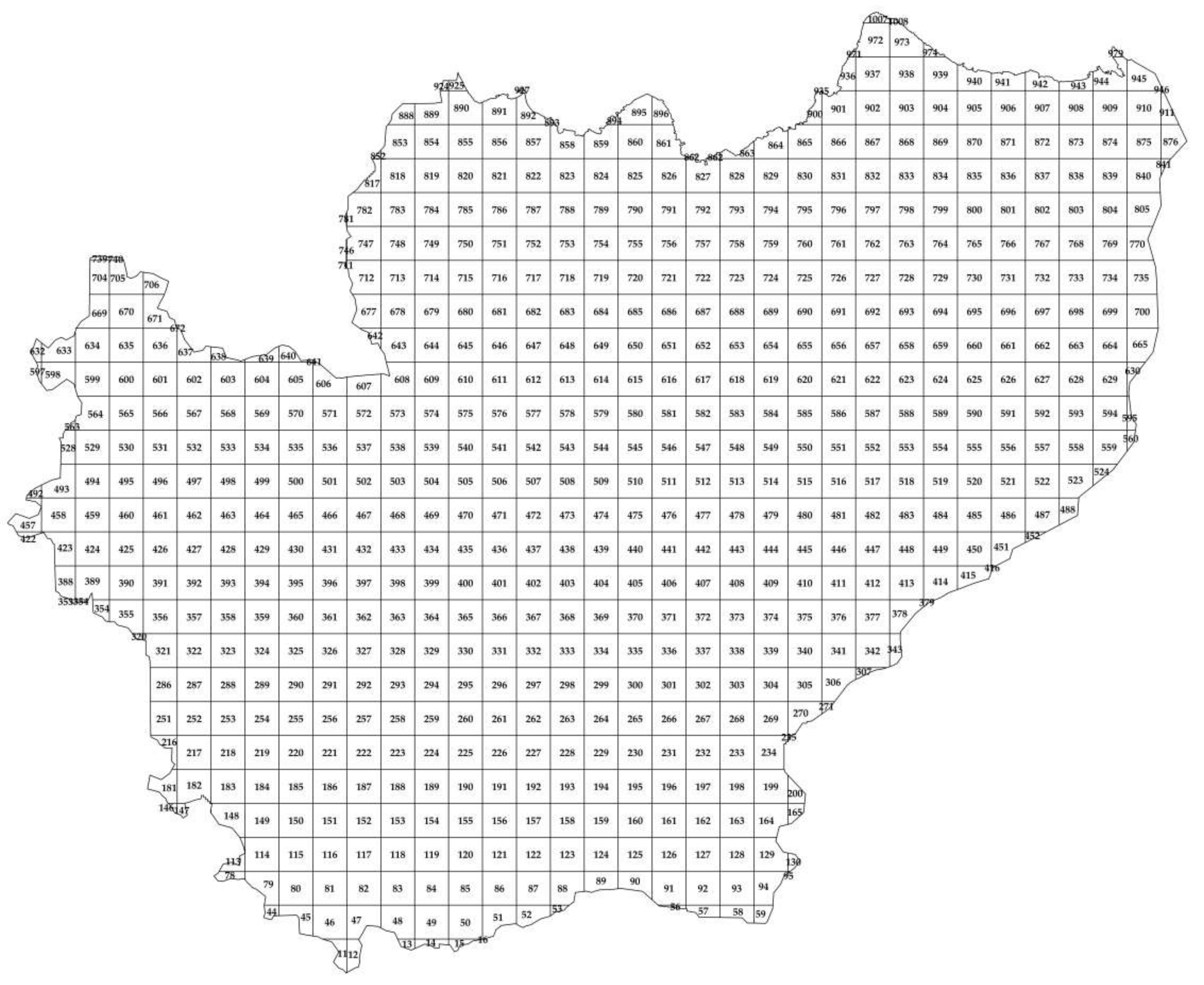
2.2.6. Calculation of Shannon’s Entropy

Quantifying urban sprawl is crucial to monitor urban development especially in areas adjacent to Ecologically Valuable Areas like MMFR. Spatial metrics are numeric measurements that quantify spatial structure and pattern of a landscape ([57,58]; as cited in [59]). Shannon’s entropy is a spatial metric commonly used to efficiently identify and characterize the degree of spatial concentration or dispersion in a geographic area [60]. The Shannon’s entropy (Hn) was computed to analyze the degree of dispersion or compactness of the spatial expansion in the MMFR watersheds and buffer zone. Shannon’s entropy (Hn) can be used to measure the degree of spatial concentration or dispersion of a geographical variable (Xi), e.g., built-up area [60,61,62]. The value of entropy ranges from 0 to log(n) [60,63]. The value of 0 [63] or closer to 0 indicates that the distribution of the built-up areas is compact while values closer to log(n) indicate that the distribution of built-up areas is dispersed [60,63]. The high values of entropy indicate the occurrence of sprawl. The halfway mark of the log(n) value is generally considered as the threshold and if the value crosses the threshold the area is considered sprawling [63].
The land cover classes from the three periods (1992, 2002, and 2015) were re-classified into two categories: built-up and non-built-up areas. In the analysis, the MMFR watersheds’ boundary was divided into 500 m by 500 m grids (Figure 3) [64] in ArcGIS 10.5 software using the Fishnet Tool. To overlay the fishnet with the MMFR watersheds and the land cover data per period, the overlay toolset (i.e., intersect) was used. Afterward, the land cover area for each class in the grids was calculated using the field calculator. The output table was converted into an Excel matrix to complete the computation of the entropy values [65]. The same procedure was used for the calculation of the entropy values for the MMFR buffer zone. The computation of the entropy was done using this formula [60]:
H n = i n p i log ( 1 p i )
where pi is the probability or proportion of occurrence of a phenomenon in the ith zone, and thus, is given by:
p i = x i / i n x i
where Xi is the area of built-up at the ith zone and n is the total number of zones. Moreover, the relative entropy was measured to scale the entropy value into a value that ranges from 0 to 1. The formula for relative entropy (H’n) [62] is:
H n = i n p i log ( 1 p i ) / log ( n )
To determine the magnitude of change of urban sprawl in the study area over time, the difference of entropy values between time t and t + 1 was measured [60,66]. A decrease in entropy over time shows that the urban development is compact while an increase in entropy shows a dispersed urban development [65]. The formula [60] for measuring the difference is:
Δ H = H n ( t + 1 ) H n ( t )
where ΔH is the change in the entropy between time (t + 1) and (t).

3. Results and Discussion

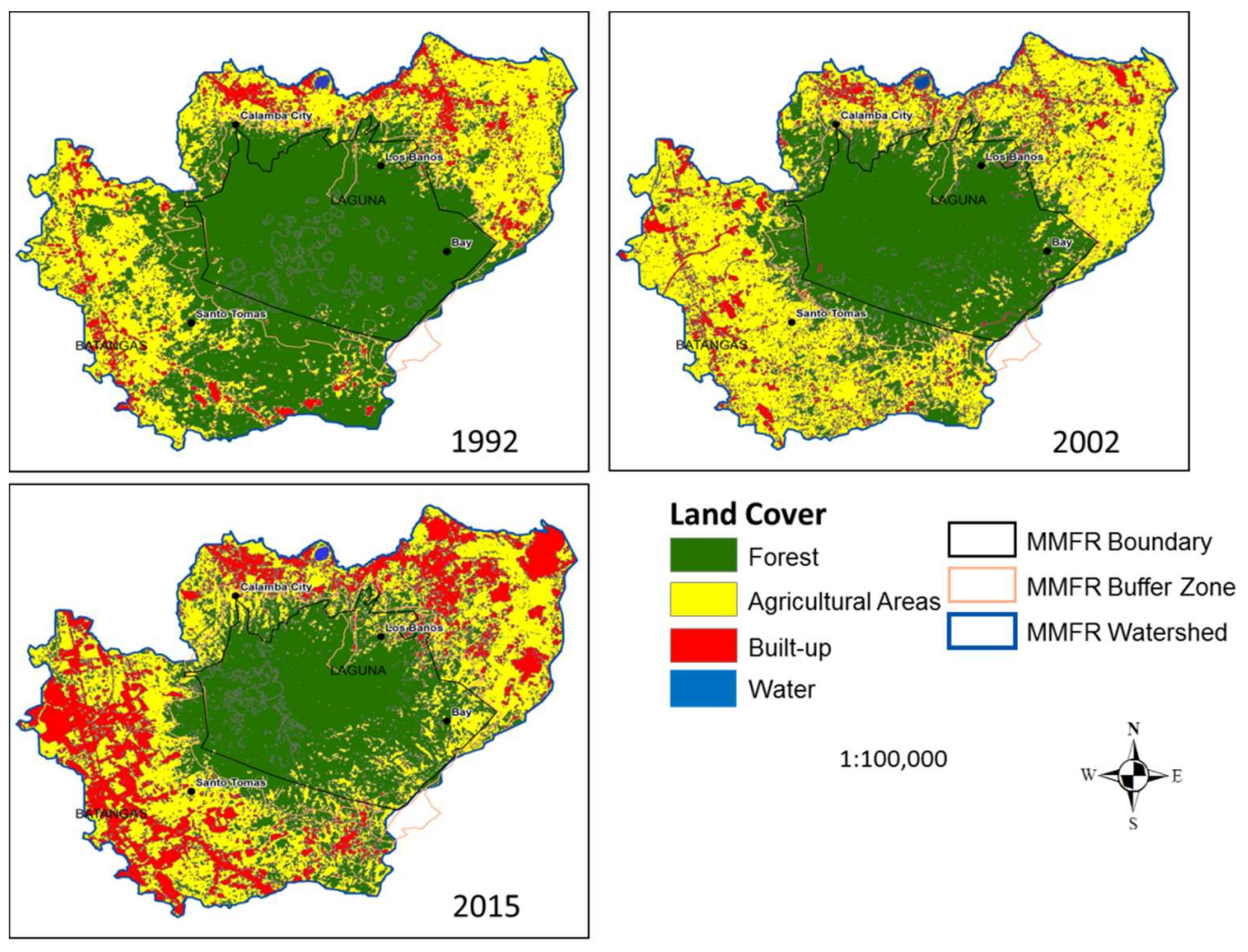
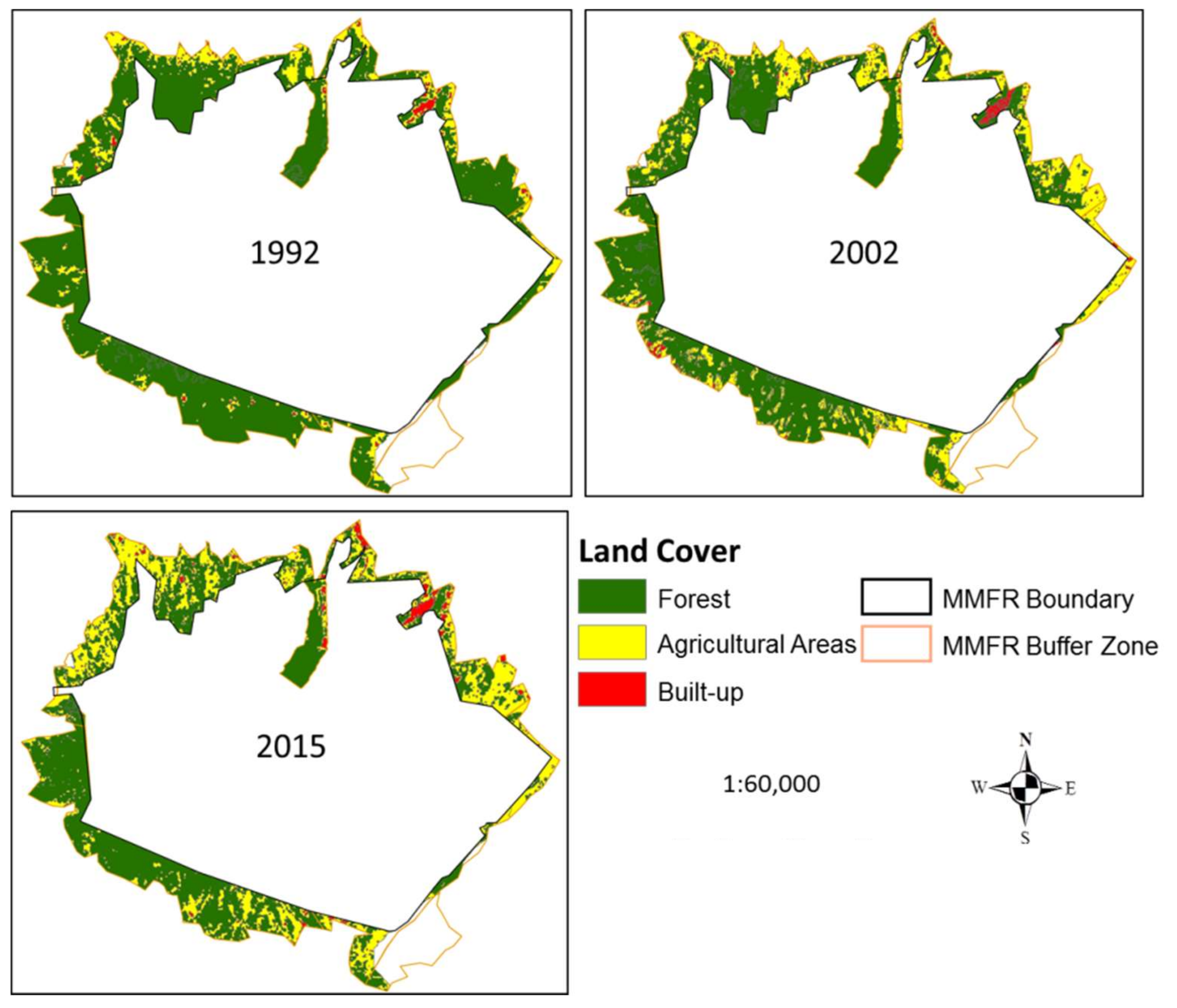
3.1. Land Classification Change Analysis

The study assessed urban sprawl in the buffer zone for MMFR from 1992 to 2015. The land cover data during the years 1992, 2002 and 2015 were initially examined to describe the historical land cover change in the MMFR watersheds and its buffer zone. The land cover classifications of MMFR watersheds and buffer zone include forest, agricultural areas, built-up, and water (Figure 4 and Figure 5). As shown in Table 4, the forest area in the MMFR watersheds had significantly decreased over time. The forest area of the MMFR watersheds decreased by as much 35% from 7884.90 has in 1992 to 5149.76 has in 2015. Moreover, there were only 1235.88 hectares of built-up areas in 1992 which more than doubled to 3368.63 hectares by 2015. During these periods, the agricultural area also increased from 5526.36 in 1992 to 6130.60 hectares in 2015. The decrease in the forest area and increase in agricultural areas and built-up areas in the MMFR watersheds can be attributed to the growing population in Bay, Los Baños, Calamba, and Sto. Tomas (Table 1). Population growth may consequently increase the need for a higher income to meet the household basic needs and in some cases, landowners may decide to give-off and trade their lands to support the growing needs of the family. Gradinaru et al. [67] stated that the landowner’s anticipation of higher profits from the sale of land with urbanization may lead to the abandonment of agricultural land to give way to built-up development.

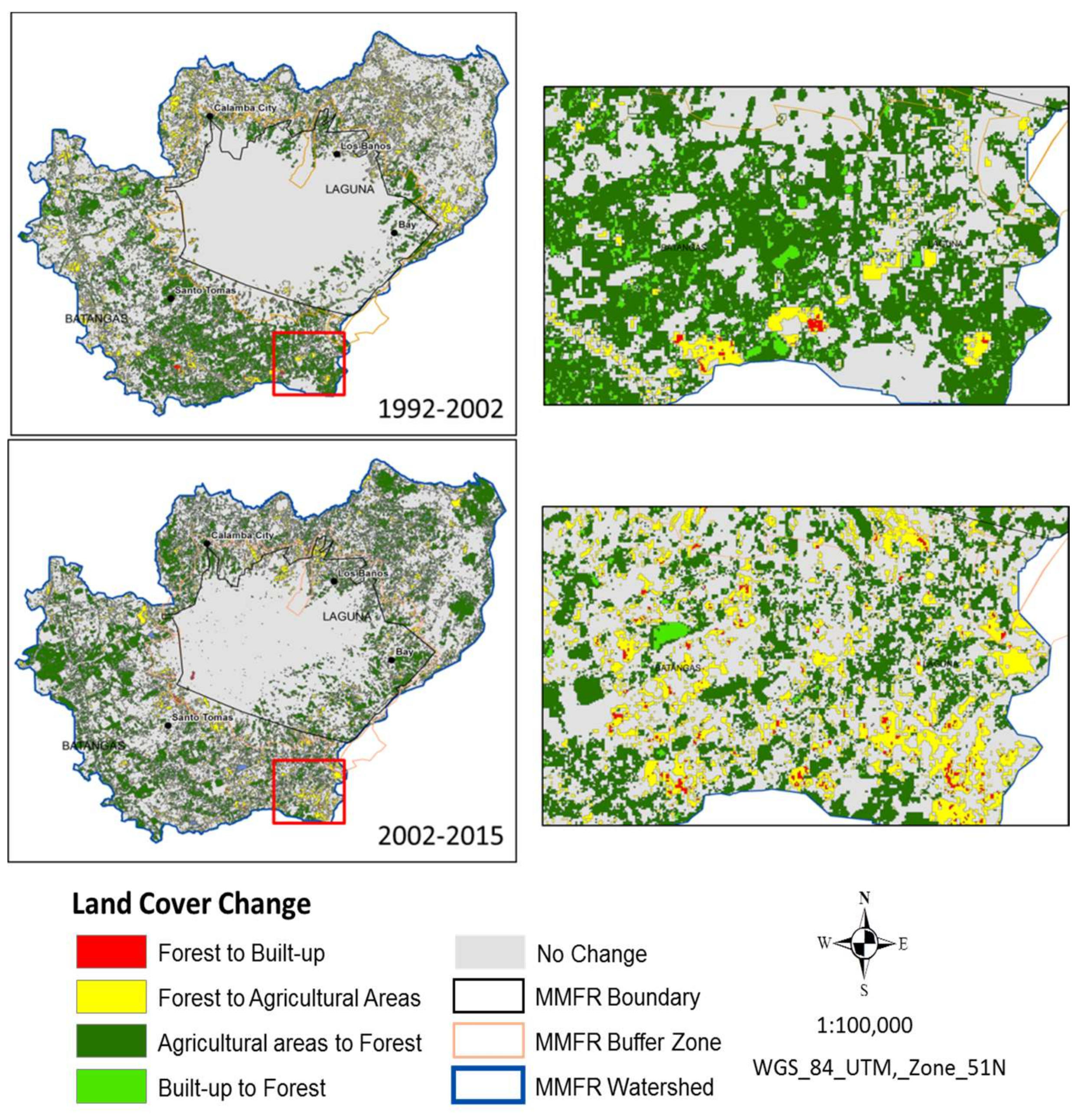
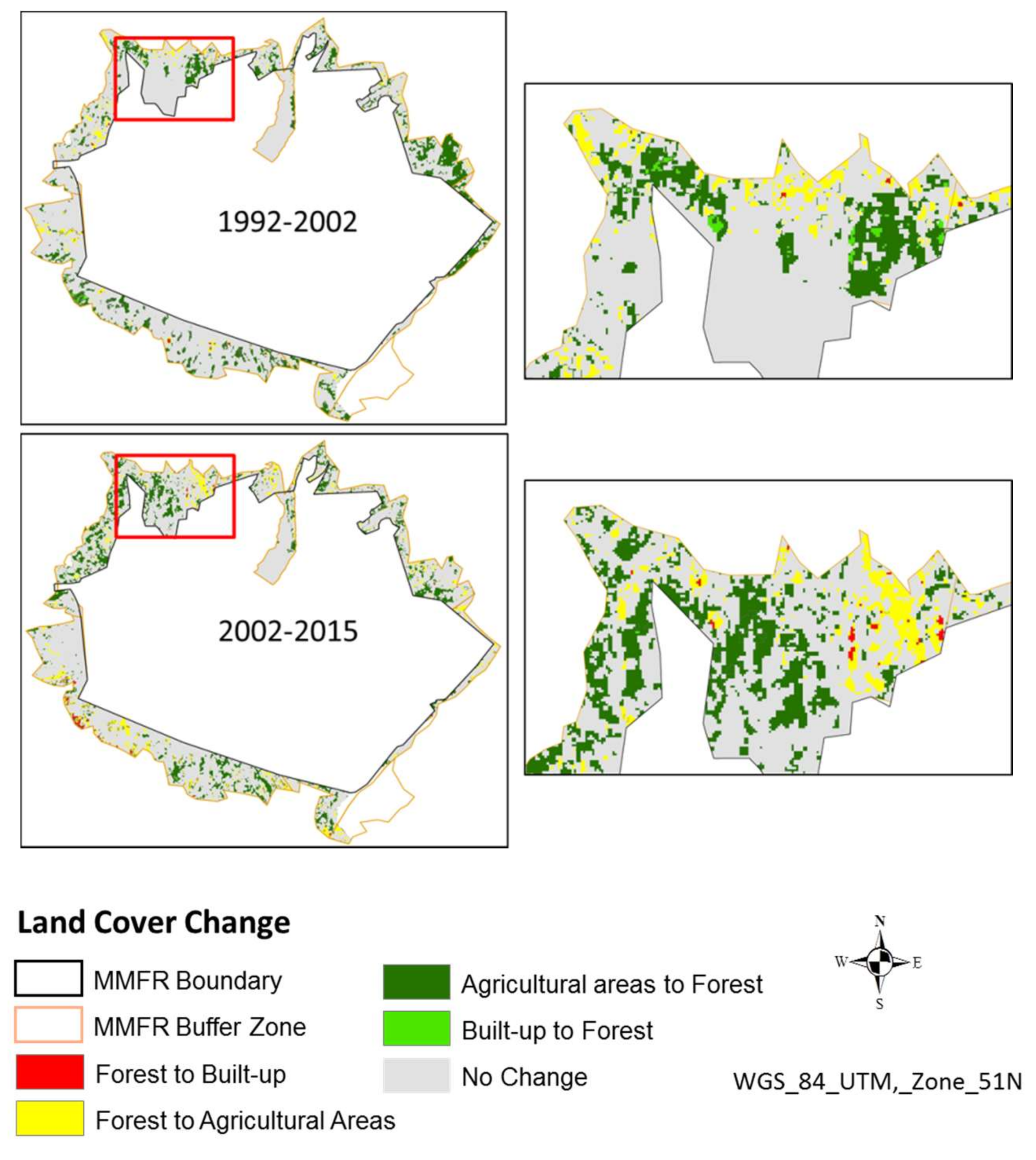
3.2. Land Cover Change Detection

Table 5 shows the land cover change in the buffer zone for MMFR. Results show that the forest area in the buffer zone decreased by 28% from 1193 hectares in 1992 to 860.15 hectares in 2015 (Figure 6 and Figure 7). The significant increase (96%) in the agricultural area in the buffer zone occurred between 1992 and 2002 when the agricultural land area increased from 225.06 ha to 441.98 ha. During these periods, 95% (from 22.67 has to 44.18 has) increased in the built-up area was also observed in the buffer zone. Panaguiton, Eustaquio, and Campo [68] stated that the increasing settlements near the forest reserve constantly threaten its stability and sustainability. They further explained that the slow but steady encroachment of communities near the borders of the forest reserve could have resulted from unclear government policies dealing with these communities and occupants. In 1998, Proclamation 1257 was issued as a response to the increasing settlements and to limit the human activities in the buffer zone of MMFR. Despite the Proclamation 1257, s. 1998, the built-up area still increased by 11% and the forest area decreased by 10% from 2002 to 2015. The authors believe that the government needs to “strengthen” Proclamation 1257 and not just a “law enforcement” considering that a legislative act is required for this.

3.3. Classification Accuracy Assessment

The indispensable procedure after various image processing techniques is the accuracy assessment [19,44,46]. Accuracy refers to the correctness of data [69]. It measures the agreement between the reference data and the output of the image classification of unknown quality [44,46,69,70]. It is ought to be done since it gives the degree of confidence and reliability of the data output [19,46] In essence, it aims to determine the percentage of pixel values that have correctly classified against the reference data. Many researchers incorporated the accuracy assessment in their studies [44,52,69,71,72,73,74]. It is important and ought to be done in the conduct of image classification for the following reasons [70,75]:
  • The legal standing of maps and reports derived from remotely-sensed data.
  • The operational use of such data for decision making e.g., watershed management.
  • The validity as input for scientific research.
In this study, a confusion matrix was utilized based on 93 sampling points with the help of ArcGIS 10.4.1 [44,45,46,74]. After image classification, at least 30 samples per class [45] were generated using the random sampling to target at least 90% overall accuracy [46]. The sampling points were the input to the accuracy assessment of the Landsat 8 classified image. Jensen [45] emphasized that the sampling points and signature data should be collected during the same period. Due to the time and resources constraints, the accuracy of the classified image was based on the available higher resolution online maps (e.g., Google Earth) [44,52,55] and other relevant secondary information available such as land cover maps from National Mapping and Resource Information Authority (NAMRIA) [56]. The matrix (Table 6) tallied the correctness of the classification generated through the application of sampling points [44,45,46,48,70,74]. The matrix was constructed based on the reference data as represented in the columns and compared against to the classified data in rows (Table 6). The major diagonal of the table shows the agreement between these two datasets.
Land cover classes such as forest, agricultural areas, built-up and water were extracted from Landsat TM, Landsat ETM+, and Landsat OLI/TIRS. The kappa and overall accuracy values of 0.91 and 93.55% were generated for the 2015 land cover map. Table 6 shows the confusion matrix with the user, producer, overall accuracies and kappa coefficient. The overall assessment result suggests that the classified land cover of MMFR Watersheds and Buffer Zone has very high accuracy and acceptability.
The accuracy of at least 85% is required for satisfactory use of land cover data for resource management [52,76]. Due to the absence of higher resolution images for 1992 and 2002, only data in 2015 were assessed accordingly [52,53]. The assumption was 2015 accuracy was sufficient to shed light on the overall accuracy of the land cover change mapping procedures [53] conducted in the study. Thus, the statistical values of the following parameters were created to evaluate the quality of the 2015 classified image [44,45,46,70,74]:
  • Overall accuracy—shows the overall quality of the data and computed as:
    Overall Accuracy = Total Correct (sum of the major diagonal)/Total number of pixels in the matrix
  • Producer’s accuracy—measures the error of omission or samples that are omitted from the correct classification since it indicates the probability that a reference sample will be correctly classified. It is called the producer’s accuracy since the analyst is concerned in mapping the Earth surface correctly. Computed as:
    Producer’s Accuracy = Total number of correct pixels in a category/Total number of pixels of that category as derived from the reference data (column total)
  • User’s Accuracy—measures the error of commission or the reliability of the map since it indicates how accurate the maps to represent what actually seen on the ground. Computed as:
    User’s Accuracy = Total number of pixels in a category/Total number of pixels that were actually classified in that category (row total)
  • Kappa Coefficient (K)—provides a more unbiased estimate of the overall agreement [48,54]. The K interpretation values range from poor to excellent agreement ranging from 0 to 1. The closer the value of K to one (1.0) the more acceptable the classification [48] and computed using the formula [45]:
    K = N∑(Xij) − ∑(rowi total)(colj total)/N2 − ∑(rowi total)(coljtotal)
    where:
    N—total number of observations;Values of K interpretation:
    Xij—sum of the major diagonal;<0No agreement
    rowi—marginal total for rowi;0.0–0.20Slight agreement
    colj—marginal total for columnj;0.21–0.40Fair agreement
    0.41–0.60Moderate agreement
    0.81–1.00Almost perfect agreement
The confusion matrix of the classified image (Landsat 8) was exported into table format (Excel file) as the basis of the quality of the classification [44] and analyzed the needed parameters (e.g., Overall Accuracy) [77].

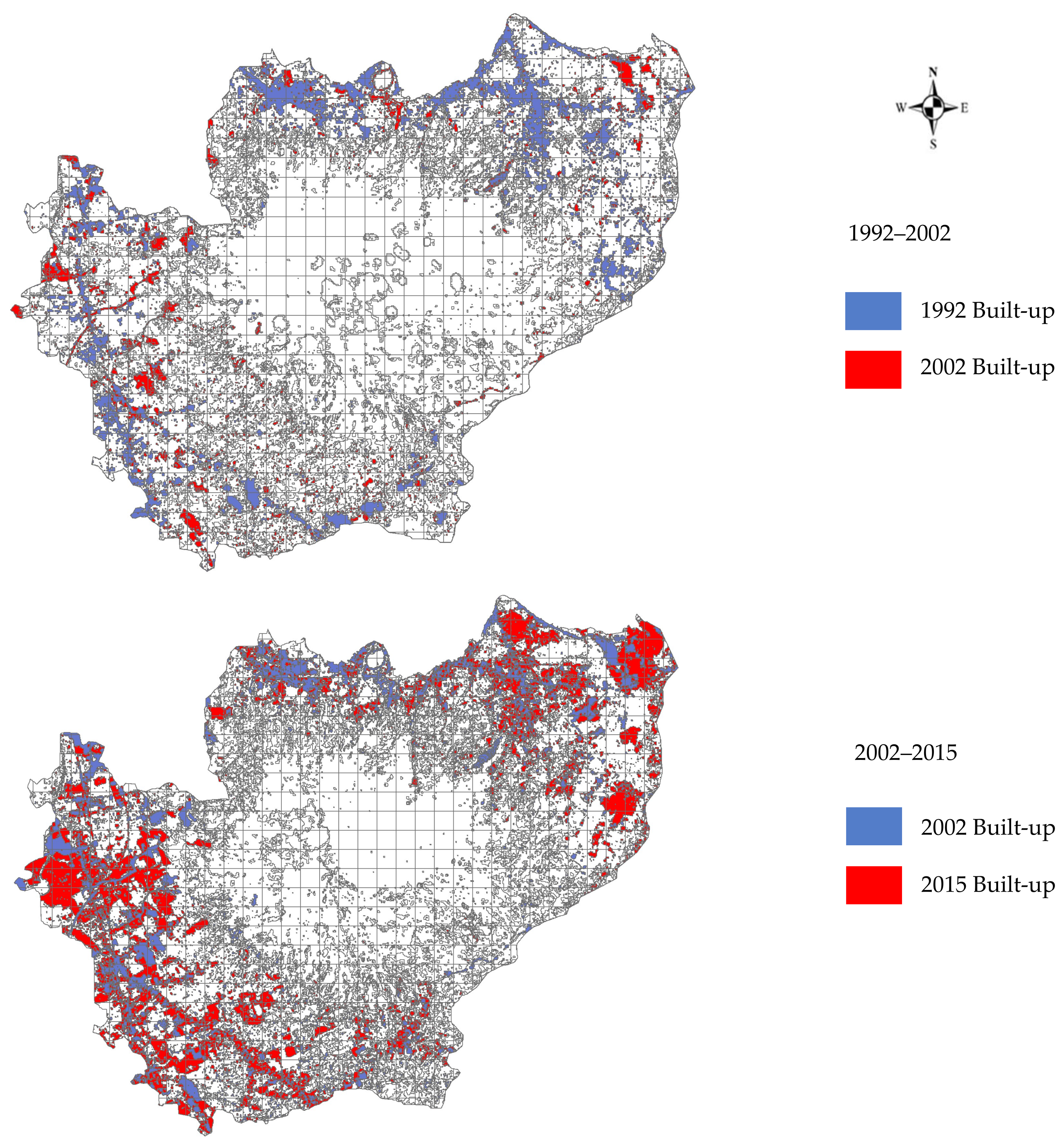
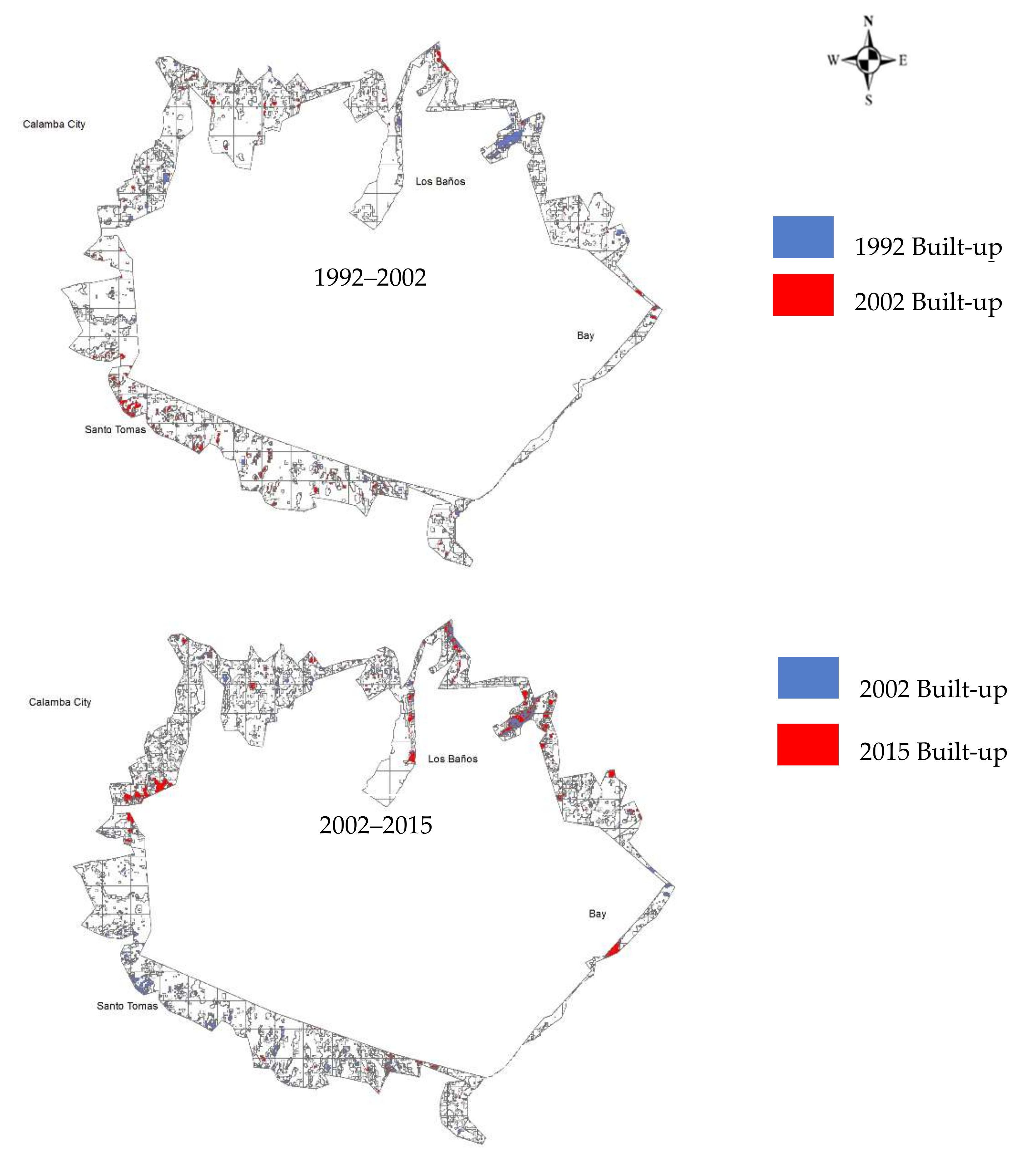
3.4. Urban Sprawl in the MMFR Watersheds

The Shannon’s entropy (Hn) was computed to analyze the degree of dispersion or compactness of the spatial expansion of built-up areas in the MMFR watersheds and buffer zone from the three periods (1992, 2002, and 2015). The results of Shannon’s Entropy analysis are summarized and illustrated in Table 7 and Figure 8, respectively. Table 7 shows that the highest value of Shannon’s entropy [Log(670)] is 2.83. The entropy results obtained for the three study periods were 2.34, 2.50, and 2.49, respectively. Moreover, the entropy values for each period is greater than the threshold value [Log(n)/2] of 1.41. Several authors stated that when the entropy value is greater than the threshold value the land development is dispersed [60,63] and sprawling [63].
However, when the magnitude of change of urban sprawl over time was calculated, a different pattern of urban sprawl in the MMFR Watersheds was observed. The results showed a difference in entropy values of 0.16 from 1992 to 2002 and −0.01 from 2002 to 2015. The decrease of entropy values was also observed in the study of Chong [68], where she explained that a decrease in entropy values over time implies a reduction on the proportion of low-intensity urban land cover across the zones resulting from the increase of high or medium intensity urban land cover or conversion to a different land cover type. An urban development is dispersed when there is an increase in entropy values over time and compact when there is a decrease in entropy values [68].

3.5. Urban Sprawl in the MMFR Buffer Zone

The results of Shannon’s entropy (Hn) for MMFR buffer zone is presented in Table 8 and Figure 9. A similar pattern of urban development was observed in the buffer zone of MMFR. The entropy values for the three periods is 1.29, 1.47, and 1.46, respectively. All Hn values were greater than the halfway mark of the log(n) value (1.085) which implies that the land development in the zone is dispersed and sprawling.
The magnitude of change of urban sprawl over time in the buffer zone of MMFR was likewise analyzed. The magnitude of change from 1992 to 2002, that is prior to the enactment of Proclamation 1257, s. 1998 up to its early years of implementation, showed a dispersed pattern of urban sprawl with a difference value of 0.18. However, from 2002 to 2015, a difference value of −0.01 was observed, which implies a compacting pattern as the human settlement in the zone increases over time. Chong [65] stated that a decrease in entropy values over time indicates that the land development in an area is becoming compact or concentrated while an increase in entropy values indicate that it is developing in a dispersed manner.

4. Conclusions

The study analyzed the urban sprawl in the MMFR watersheds and its buffer zone using time series assessment based on Landsat data. The land cover was characterized through a supervised classification approach. The Shannon’s entropy (Hn) was also calculated to describe the spatial patterns of urban sprawl in the area. Results showed that the land cover within the buffer zone of MMFR changes from 1992 to 2015 with a 117% increase in built-up areas despite the existence of policies concerning the management of the zone. In 2015, the total built-up area in the buffer zone was 49.22 ha representing 3.4% of the total area of the buffer zone. From 2002 to 2015, a few years after the enactment of Proclamation 1257, s. 1998, the magnitude of change of urban sprawl in the buffer zone shows to be compact as the human settlement in the area increases. The study suggests that the assessment and monitoring of urban sprawl in the buffer zone be conducted regularly using remote sensing and GIS to effectively implement policies, e.g., Proclamation 1257, s. 1998 and other related laws and to avoid further disturbance, encroachment, and pressure. The study also suggests that a policy gap analysis need to be conducted to understand more the pattern of human settlement in the buffer zone of MMFR in relation to the implementation of Proclamation 1257, s. 1998 and other related laws. The utilization of remote sensing data and GIS technology should also be considered in the assessment and monitoring of urban sprawl in ecologically valuable areas as their applicability and importance were showcased in this study.

Author Contributions

Conceptualization, M.S. and N.H.; Data Curation, M.S., N.H. and A.J.H.; Formal Analysis, M.S. and N.H.; Methodology, M.S., N.H. and A.J.H.; Project Administration, M.S. and N.H.; Resources, M.S. and A.A.; Supervision, C.T.J.; Validation, M.S. and N.H.; Visualization, M.S. and N.H.; Writing—Original Draft, M.S. and N.H.; Writing—Review and Editing, M.S., N.H., R.G. and C.T.J.

Funding

This research received no external funding.

Acknowledgments

The authors wish to express their gratitude to UPLB-MCME for the MMFR digital maps, NAMRIA for the provision of software (e.g., ENVI and ArcGIS), USGS for the free-access and downloadable Landsat satellite images, and Rico Ancog for his valuable insights. Also, to the Philippines Commission on Higher Education (CHED) for sponsoring the conference registration fee on the 2018 International Conference on Sustainable Environmental Technologies (ICSET) and for funding the publication fee, and to the ICSET organizer for facilitating the publication of this paper.

Conflicts of Interest

The authors declare no conflict of interest.

References

  1. Esbah, H.; Deniz, B.; Kara, B.; Atatanir, L. Monitoring Urban Development Near a protected area. In Proceedings of the Urban Remote Sensing Joint Event, Paris, France, 11–13 April 2007; pp. 1–6. [Google Scholar] [CrossRef]
  2. Daniel, T.C.; Muhar, A.; Arnberger, A.; Aznar, O.; Boyd, J.W.; Chan, K.M.A.; Costanza, R.; Elmqvist, T.; Flint, C.G.; Gobster, P.H. Contributions of cultural services to the ecosystem services agenda. Proc. Natl. Acad. Sci. USA 2012, 109, 8812–8819. [Google Scholar] [CrossRef] [PubMed] [Green Version]
  3. Pressey, R.L.; Humphries, C.J.; Margules, C.R.; Vane-Wright, R.I.; Williams, P.H. Beyond opportunism: Key principles for systematic reserve selection. Trends Ecol. Evol. 1993, 8, 124–128. [Google Scholar] [CrossRef]
  4. Meffe, G.; Carroll, R. Principles of Conservation Biology; Sinauer Press: Sunderland, UK, 1997. [Google Scholar]
  5. Howard, P.C.; Viskanic, P.; Davenport, T.R.B.; Kigenyi, F.W.; Baltzer, M.; Dickinson, C.J.; Lwanga, J.S.; Matthews, R.A.; Balmford, A. Complementarity and the use of indicator groups for reserve selection in Uganda. Nature 1998, 39, 472–475. [Google Scholar] [CrossRef]
  6. Götmark, F.; Söderlundh, H.; Thorell, M. Buffer zones for forest reserves: Opinions of landowners and conservation value of their forest around nature reserves in southern Sweden. Biodivers. Conserv. 2000, 9, 1377–1390. [Google Scholar] [CrossRef]
  7. Tryzna, T. Global Urbanization and Protected Areas: Challenges and Opportunities Posed by a Major Factor of Global Change- and Creative Ways of Responding; California Institute of Public Affairs: Sacramento, CA, USA, 2007; 52p. [Google Scholar]
  8. Wang, G.; Jiang, G.; Zhou, Y.; Liu, Q.; Ji, Y.; Wang, S.; Chen, S.; Liu, H. Biodiversity Conservation in a fast-growing metropolitan area in China: A case study of plant diversity in Beijing. Biodivers. Conserv. 2007, 16, 4025–4038. [Google Scholar] [CrossRef]
  9. Mutuga, F. The Effect of Urbanization on Protected areas: The Impact of Urban Growth on a Wildlife Protected Area: A Case Study of Nairobi National Park. Master’s Thesis, IIIEE Lund University, Lund, Sweden, June 2009. Available online: http://lup.lub.lu.se/luur/download?func=downloadFile&recordOId=1513631&fileOId=1513632/ (accessed on 26 November 2017).
  10. The Environmental Literacy Council. Urban Sprawl. Available online: https://enviroliteracy.org/land-use/urbanization/urban-sprawl/ (accessed on 28 November 2017).
  11. Joppa, L.N.; Loarie, S.R.; Pimm, S.L. On Population Growth near Protected Areas. PLoS ONE 2009, 4, e4279. [Google Scholar] [CrossRef]
  12. Beatley, T. Land Development and endangered species: Emerging conflicts. In The Sustainable Urban Development Reader; Wheeler, S.M., Beatley, T., Eds.; Routledge: London, UK, 2004; pp. 116–199. [Google Scholar]
  13. Rathore, B.M.S. Joint management options for protected areas. In People and Protected Areas: Towards Participatory Conservation in India; Kothari, A., Singh, N., Suri, S., Eds.; Sage: New Delhi, India, 1996. [Google Scholar]
  14. McDonald, R.; Kareiva, P.; Forman, R. The implications of current and future urbanization for global protected areas and biodiversity conservation. Biodivers. Conserv. 2008, 141, 1695–1703. [Google Scholar] [CrossRef]
  15. Biswal, A.; Jeyaram, A.; Mukherjee, S.; Kumar, U. Analysis of Temporal and Spatial Changes in the Vegetation Density of Similipal Biosphere Reserve in Odisha (India) Using Multitemporal Satellite Imagery. Int. J. Ecol. 2013, 368419. [Google Scholar] [CrossRef]
  16. Sunar Erbek, A.; Ulubay, A.; Maktav, D.; Yağiz, E. The use of satellite image maps for urban planning in Turkey. Int. J. Remote Sens. 2005, 26, 775–784. [Google Scholar] [CrossRef]
  17. Willis, K.S. Remote sensing change detection for ecological monitoring in United States protected areas. Biodivers. Conserv. 2015, 182, 233–242. [Google Scholar] [CrossRef]
  18. Mohammady, S.; Delavar, M.R. Urban sprawl assessment and modeling using Landsat images and GIS. Model. Earth Syst. Environ. 2016, 2, 155. [Google Scholar] [CrossRef]
  19. Franklin, S.E. Remote Sensing for Sustainable Forest Management; CRC Press LLC: Boca Raton, FL, USA, 2001. [Google Scholar]
  20. Lopez, J.M.R.; Heider, K.; Scheffran, J. Frontiers of Urbanization: Identifying and Explaining Urbanization Hotspots in the South of Mexico City using Human and Remote Sensing. Appl. Geogr. 2017, 79, 1–10. [Google Scholar] [CrossRef]
  21. Jensen, J.R.; Cowen, D.C. Remote sensing of urban/suburban infrastructure and socio-economic attributes. Photogramm. Eng. Remote Sens. 1999, 65, 611–622. [Google Scholar]
  22. Brandt, J.; Kuemmerle, T.; Li, H.; Ren, G.; Zhu, J.; Radeloff, V. Using Landsat imagery to map forest change in southwest China in response to the national logging ban and ecotourism development. Remote Sens. Environ. 2012, 121, 358–369. [Google Scholar] [CrossRef]
  23. Republic Act 6967. An Act to Vest Control, Jurisdiction and Administration of the Forest Reserve in Mount Makiling in the University of the Philippines in Los Baños. Available online: http://www.officialgazette.gov.ph/1990/10/15/republic-act-no-6967-2/ (accessed on 24 November 2017).
  24. Bantayan, N.C.; Abraham, E.R.G.; Fernando, E.S. Geodatabase Development for Forest Restoration and Biodiversity Conservation in the Mt. Makiling Forest Reserve, Philippines. Philipp. Agric. Sci. 2008, 91, 365–371. [Google Scholar]
  25. Lapitan, P.; Castillo, M.; Pampolina, N. Mt. Makiling Forest Reserve Spring Well of Natural and Knowledge Resources of the Philippines; ASEAN-Korea Environmental Cooperation Unit (AKECU), National Instrumentation Center for Environmental Management, College of Agriculture and Life Sciences, Seoul National University: Seoul, Korea, 2011; p. 9. ISBN 978-89-6558-046-1. [Google Scholar]
  26. Lapitan, P.G. Restoration of Mt Makiling—A Biodiversity Hotspot and Ecotourism Destination in the Philippines. In Proceedings of the IUFRO Conference on Forest Landscape Restoration, Seoul, Korea, 14–19 May 2007; Stanturf, J., Ed.; Korean Forest Research Institute: Seoul, Korea, 2007. [Google Scholar]
  27. Vallesteros, A.P. GIS-Based Determination of Socioeconomic Variables Affecting Land-Use Change in Mt. Makiling Forest Reserve, Philippines. Master’s Thesis, UPLB College, Laguna, Philippines, 2002. [Google Scholar]
  28. Combalicer, M.; Kim, D.; Lee, D.K.; Combalicer, E.; Cruz, R.V.; Im, S. Changes in the forest landscape of Mt. Makiling Forest Reserve, Philippines. For. Sci. Technol. 2011, 7, 60–67. [Google Scholar] [CrossRef]
  29. Ranada, P. Mt Makiling Named ASEAN Heritage Park. October 4 2013. Available online: http://www.rappler.com/nation/40522-makiling-asean-heritage-park/ (accessed on 31 March 2017).
  30. Combalicer, E.; Im, S. Change Anomalies of Hydrologic Responses to Climate Variability and Land Use Changes in the Mt. Makiling Forest Reserve. J. Environ. Sci. Manag. 2012, 15, 1–13. [Google Scholar]
  31. Proclamation 1257, s. 1998. Designating Certain Areas Surrounding the Makiling Forest Reserve as Buffer Zone and Prescribing Guidelines Thereof. Available online: http://www.officialgazette.gov.ph/2007/03/23/proclamation-no-1257-s-2007/ (Accessed on 30 March 2017).
  32. Pulhin, J.; Tapia, M. History of a Legend: Managing the Makiling Forest Reserve. 2005. Available online: http://www.fao.org/tempref/docrep/fao/007/AE542e/ae542e23.pdf (accessed on 15 October 2016).
  33. Lusterio, R. Policy-Making for Sustainable Development: The Case of Makiling Forest Reserve. Philippine Social Sciences Review, [S.l.], June 2011. ISSN 0031-7802. Available online: http://ovcrd.upd.edu.ph/pssr/article/view/2123/ (Accessed on 24 November 2017).
  34. Philippine Statistics Authority (PSA). Philippine Population Density (Based on the 2015 Census of Population). 2015. Available online: https://psa.gov.ph/sites/default/files/attachments/hsd/pressrelease/2015%20Population%20Density_web.xlsx/ (Accessed on 22 November 2017).
  35. Proclamation Order No. 349, s. 2000. Designating and Declaring the Municipality of Los Baños, Laguna as a Special Science and Nature City of the Philippines. Available online: http://www.officialgazette.gov.ph/2000/08/07/proclamation-order-no-349-s-2000/ (Accessed on 24 November 2017).
  36. Bagarino, R.T. A Spatial Analysis of Population Growth and Urbanization in Calamba City Using GIS. J. Nat. Stud. 2015, 14, 1–13. Available online: http://www.journalofnaturestudies.org/files/JNS14-2/14(2)%201-13%20Bagarinao-fullpaper.pdf (accessed on 24 November 2017).
  37. Philippine Statistics Authority (PSA). 2010 Census of Population and Housing Philippines. 2010. Available online: https://psa.gov.ph/sites/default/files/attachments/hsd/article/Table%202_0.pdf/ (accessed on 24 November 2017).
  38. Department of Interior and Local Government CALABARZON. Sto. Tomas. 2014. Available online: http://calabarzon.dilg.gov.ph/89-lgus/batangas?start=8/ (accessed on 24 November 2017).
  39. Landsat Satellite Image (July 29, 2015; Landsat 8 OLI/TIRS) Downloaded Dated October 2017 Courtesy of US Geological Survey Science of a Changing World. Available online: https://earthexplorer.usgs.gov/ (accessed on 18 October 2017).
  40. Landsat Satellite Image (January 26, 1992; Landsat TM) Downloaded Dated October 2017 Courtesy of US Geological Survey Science of a Changing World. Available online: https://earthexplorer.usgs.gov/ (accessed on 18 October 2017).
  41. Landsat Satellite Image (April 04, 2002; Landsat 7 ETM+) Downloaded Dated October 2017 Courtesy of US Geological Survey Science of a Changing World. Available online: https://earthexplorer.usgs.gov/ (accessed on 18 October 2017).
  42. Chander, G.; Markham, B. Revised Landsat-5 TM Radiometric Calibration Procedures and Postcalibration Dynamic Ranges. IEEE Trans. Geosci. Remote Sens. 2003, 41, 2674–2677. [Google Scholar] [CrossRef]
  43. Dewa, R.P.; Danoedoro, P. The effect of image radiometric correction on the accuracy of vegetation canopy density estimate using several Landsat-8 OLI’s vegetation indices: A case study of Wonosari area, Indonesia. IOP Conf. Ser. Earth Environ. Sci. 2017, 54, 012046. [Google Scholar] [CrossRef] [Green Version]
  44. Ghebrezgabher, M.G.; Yan, T.; Yang, X.; Wang, X.; Khan, M. Extracting and analyzing forest and woodland cover change in Eritrea based on Landsat data using supervised classification. Egypt. J. Remote Sens. Space Sci. 2016, 19, 37–47. [Google Scholar] [CrossRef]
  45. Jensen, J.R. Introductory Digital Image Processing: A Remote Sensing Perspective; Prentice Hall Inc.: Upper Saddle River, NJ, USA, 1996; pp. 379–386. [Google Scholar]
  46. Richards, J.A.; Jia, X. Remote Sensing Digital Image Analysis, an Introduction, 4th ed.; Springer: Canberra, Australia, 2005. [Google Scholar]
  47. Google Earth Pro V. 7.3.2.5491 (July 20, 2015). Mount Makiling Forest Reserve, Los Baňos, Laguna, Philippines, Latitude 14008′03.61″N, Longitude 121012′12.98″E, Elevation 2785ft, Eye Alt 11816ft, Digital Globe 2018. Available online: https://www.google.com/earth/download/gep/agree.html (accessed on 24 October 2017).
  48. Natarajan, K.; Latva-Käyrä, P.; Zyadin, A.; Pelkonen, P. New methodological approach for biomass resource assessment in India using GIS application and land use/land cover (LULC) maps. Renew. Sustain. Energy Rev. 2016, 63, 256–268. [Google Scholar] [CrossRef]
  49. Scharsich, V.; Mtata, K.; Hauhs, M.; Lange, H.; Bogner, C. Analysing land cover and land use change in the Matobo National Park and surroundings in Zimbabwe. Remote Sens. Environ. 2017, 194, 278–286. [Google Scholar] [CrossRef]
  50. Food and Agriculture Organization (FAO). Global Forest Resources Assessment. Terms and Definitions. Forest Resources Assessment Programme; Working Paper 144/E; FAO: Rome, Italy, 2010; Available online: http://www.fao.org/docrep/014/am665e/am665e00.pdf. (accessed on 10 October 2017).
  51. Congalton, R.G. A review of assessing the accuracy of classifications of remotely sensed data. Remote Sens. Environ. 1991, 37, 35–46. [Google Scholar] [CrossRef]
  52. Zhang, X.; Pan, D.; Chen, J.; Zhan, Y.; Mao, Z. Using longtime series of Landsat data to monitor impervious surface dynamics a case study in the Zhoushan Islands. J. Appl. Remote Sens. 2013, 7, 1–14. [Google Scholar] [CrossRef]
  53. Wasige, J.E.; Groen, T.A.; Smaling, E.S.; Jetten, V. Monitoring basin-scale land cover changes in Kagera Basin of Lake Victoria using ancillary data and remote sensing. Int. J. Appl. Earth Obs. Geoinf. 2013, 21, 32–42. [Google Scholar] [CrossRef]
  54. Nurwanda, A.; Zain, A.F.; Rustiadi, E. Analysis of land cover changes and landscape fragmentation in Batanghari Regency, Jambi Province. Procedia Soc. Behav. Sci. 2016, 227, 87–94. [Google Scholar] [CrossRef]
  55. Paquit, J.C.; Mindaña, F.N.W. Modeling the spatial pattern of carbon stock in Central Mindanao University using inVEST tool. J. Biodivers. Environ. Sci. 2017, 10, 103–113. [Google Scholar]
  56. National Mapping and Resource Information Authority. 2017. Available online: http://www.namria.gov.ph/ (accessed on 16 October 2017).
  57. O’Neill, R.V.; Krummel, J.R.; Gardner, R.H.; Sugihara, G.; Jackson, B.; Deangelis, D.L.; Milne, B.T.; Turner, M.G.; Zygmunt, B.; Christensen, S.W.; et al. Indices of landscape pattern. Landsc. Ecol. 1988, 1, 153–162. [Google Scholar] [CrossRef]
  58. McGarigal, K.; Marks, B.J. FRAGSTATS: Spatial Pattern Analysis Program for Quantifying Landscape Structure; General Technical Report PNW-351; USDA Forest Service: Washington, DC, USA, 1995. [Google Scholar]
  59. Bhatta, B.; Saraswati, S.; Bandyopadhyay, D. Urban sprawl measurement from remote sensing data. Appl. Geogr. 2010, 30, 731–740. [Google Scholar] [CrossRef]
  60. Yeh, A.; Li, X. Measurement and Monitoring of Urban Sprawl in a Rapidly Growing Region Using Entropy. Photogram. Eng. Remote Sens. 2001, 67, 83–90. Available online: https://www.asprs.org/wp-content/uploads/pers/2001journal/january/2001_jan_83-90.pdf (accessed on 30 November 2017).
  61. Theil, H. Economics and Information Theory; North-Holland: Amsterdam, The Netherlands, 1967; p. 488. [Google Scholar]
  62. Thomas, R.W. Information Statistics in Geography, Geo Abstracts; University of East Anglia: Norwich, UK, 1981; p. 42. [Google Scholar]
  63. Dadras, M.; Shafri, H.Z.M.; Ahmad, N.; Pradhan, B.; Safarpour, S. Six decades of urban growth using remote sensing and GIS in the city of Bandar Abbas, Iran. IOP Conf. Ser.: Earth Environ. Sci. 2014, 20, 012007. [Google Scholar] [CrossRef] [Green Version]
  64. Singh, B. Urban Growth Using Shannon’s Entropy: A Case Study of Rohtak City. Int. J. Adv. Remote Sens. GIS 2014, 3, 544–552. Available online: http://technical.cloud-journals.com/index.php/IJARSG/article/view/Tech-237/ (accessed on 2 December 2017).
  65. Chong, C. Comparison of Spatial Data Types for Urban Sprawl Analysis Using Shannon’s Entropy. Master’s Thesis, University of Southern California, Angeles, CA, USA, May 2017. Available online: https://spatial.usc.edu/wp-content/uploads/2017/02/Chong_Cora.pdf (accessed on 30 November 2017).
  66. Effat, H.; ElShobaki, M. Modeling and Mapping of Urban Sprawl Pattern in Cairo Using Multi-Temporal Landsat Images, and Shannon’s Entropy. Adv. Remote Sens. 2015, 4, 303–318. [Google Scholar] [CrossRef]
  67. Grădinaru, S.R.; Iojă, C.; Onose, D.; Gavrilidis, A.; Pătru-Stupariu, I.; Kienast, F. Hersperger, A. Land abandonment as a precursor of built-up development at the sprawling periphery of former socialist cities. Ecol. Indic. 2015, 57, 305–313. [Google Scholar] [CrossRef]
  68. Panaguiton, L.; Eustaquio, R.; Campo, P. Urban Sprawl Assessment in the Mount Makiling Forest Reserve Using Remote Sensing and GIS Technologies. In Proceedings of the 19th Conference on Remote Sensing 1998, Manila, Philippines, 16–20 November 1998; p. E-6. [Google Scholar]
  69. Joshi, R.R.; Warthe, M.; Dwivedi, S.; Vijay, R.; Chakrabarti, T. Monitoring changes in land use land cover of Yamuna riverbed in Delhi: A multi-temporal analysis. Int. J. Remote Sens. 2011, 32, 9547–9558. [Google Scholar] [CrossRef]
  70. Congalton, R.G. Remote sensing brief, accuracy assessment: A user’s perspective. Photogram. Eng. Remote Sens. 1986, 52, 397–399. [Google Scholar]
  71. Comber, A.; Fisher, P.; Brunsdon, C.; Khmag, A. Spatial analysis of remote sensing image classification accuracy. Remote Sens. Environ. 2012, 127, 237–246. [Google Scholar] [CrossRef] [Green Version]
  72. Barrett, B.; Nitze, I.; Green, S.; Cawkwell, F. Assessment of multi-temporal, multi-sensor radar and ancillary spatial data for grasslands monitoring in Ireland using machine learning approaches. Remote Sens. Environ. 2014, 152, 109–124. [Google Scholar] [CrossRef] [Green Version]
  73. Baumann, M.; Ozdogan, M.; Wolter, P.T.; Krylov, A.; Vladimirova, N.; Radeloff, V.C. Landsat remote sensing of forest windfall disturbance. Remote Sens. Environ. 2014, 143, 171–179. [Google Scholar] [CrossRef]
  74. Churches, S.E.; Wampler, P.J.; Sun WSmith, A.J. Evaluation of forest cover estimates for Haiti using supervised classification of Landsat data. Int. J. Appl. Earth Obs. Geoinf. 2014, 30, 203–216. [Google Scholar] [CrossRef] [Green Version]
  75. Congalton, R.G.; Green, K. Assessing the Accuracy of Remotely Sensed Data—Principles and Practices, 2nd ed.; CRC Press, Taylor & Francis Group: Boca Raton, FL, USA, 2008. [Google Scholar]
  76. Anderson, J.F.; Hardy, E.E.; Roach, J.T.; Witmer, R.E. A Land Use and Land Cover Classification System for Use with Remote Sensor Data; U.S. Geological Survey Professional Paper 964; U.S. Geological Survey: Washington, DC, USA, 1976; pp. 28–32. [Google Scholar]
  77. Foody, G.M. Status of land cover classification accuracy assessment. Remote Sens. Environ. 2002, 80, 185–201. [Google Scholar] [CrossRef]
Figure 1. Geographical location of Mount Makiling Forest Reserve (MMFR) watersheds and buffer zone using the 2015 Landsat 8 [39].
Environments 06 00009 g001
Figure 2. Flowchart for urban sprawl detection and assessment.
Environments 06 00009 g002
Figure 3. The Mount Makiling Forest Reserve (MMFR) Watersheds divided into 500 m × 500 m grids using the Fishnet Tool.
Environments 06 00009 g003
Figure 4. Land Cover Maps of MMFR Watersheds in 1992, 2002 and 2015 generated using the Supervised Classification Approach.
Environments 06 00009 g004
Figure 5. Land Cover Maps of MMFR Buffer Zone in 1992, 2002 and 2015 generated using the Supervised Classification Approach.
Environments 06 00009 g005
Figure 6. Change Maps of the MMFR Watersheds from 1992–2002 and 2002–2015. The two insets show the same zoomed area for its land cover change.
Environments 06 00009 g006
Figure 7. Change Maps of MMFR Buffer Zone from 1992–2002 and 2002–2015. The two insets show the same zoomed area for its land cover change.
Environments 06 00009 g007
Figure 8. Urban Sprawl in MMFR Watersheds from 1992–2002 and 2002–2015.
Environments 06 00009 g008
Figure 9. Urban Sprawl in MMFR Buffer Zone from 1992–2002 and 2002–2015.
Environments 06 00009 g009
Table 1. Population, Land Area and Population Density of Areas portions of which are covered by the Mount Makiling Forest Reserve [34].
Municipality/CityPopulationLand Area (km²)Population Density (person/km²)
Bay, Laguna62,14342.661457
Calamba City, Laguna454,486149.503040
Los Baños, Laguna112,00854.222066
Santo Tomas, Batangas179,84495.411885
Table 2. Different data used in the study.
Data SensorDate AcquiredScale/ResolutionData SourceProjection
MMFR Watersheds (shapefile)-12 November 2017-UPLB-MCMEWGS 84 UTM 51N
MMFR Buffer Zone Boundary (shapefile)-12 November 2017-UPLB-MCMEWGS 84 UTM 51N
MMFR Boundary (shapefile)-12 November 2017-UPLB-MCMEWGS 84 UTM 51N
Landsat 5MSS26 January 199230 mUSGS Earth ExplorerWGS 84 UTM 51N
Landsat 7ETM+4 April 200230 mUSGS Earth ExplorerWGS 84 UTM 51N
Landsat 8OLI/TIRS29 July 201530 mUSGS Earth Explorer SurveyWGS 84 UTM 51N
MSS—Multi-spectral Scanner. ETM+—Enhanced Thematic Mapper Plus. OLI/TIRS—Operational Land Imager/Thermal Infrared Sensor. UPLB-MCME—Universitey of the Philippines Los Baños-Makiling Center for Mountain Ecosystems. USGS—United States Geological Survey. WGS—World Geodetic System. UTM—Universal Transverse Mercator.
Table 3. Land cover classes and descriptions used in the study (Source: [50]).
I.D. NO.Land Cover ClassesFAO’s FRA 2010
1ForestVegetation or tree cover more than 5 m in height with more than two species, and the canopy or crown ranges from 10% to 40% for open forest and above 40% for closed forest and the forest includes the riverine and mangrove.
2Agricultural Areas/LandAll other non-forested land, including grassland, agricultural land, and cropland.
3Built-upAll other non-forested land, such as urban areas, human settlements and road networks.
4WaterInland water bodies generally include major rivers, lakes and water reservoirs.
Table 4. Land Cover and Percentage of Land Cover Change in Mount Makiling Forest Reserve Watersheds in three periods: 1992, 2002, and 2015.
Class1992200220151992–2002 Area Changed (ha)2002–2015 Area Changed (ha)
Class Area (ha)%Class Area (ha)%Class Area (ha)%
Forest7884.9053.775783.6339.445149.7635.12−2101.28−633.87
Agricultural Areas5526.3637.687466.0250.916130.6041.801939.66−1335.42
Built-up1235.888.431398.609.543368.6322.97162.721970.0325
Water17.280.1217.280.1216.540.110.00−0.7425
Total14,665.00100.0014,665.00100.0014,665.00100.00--
(−) indicates decrease.
Table 5. Land cover and Percentage of Land Cover Change in Buffer Zone for Mount Makiling Forest Reserve Watersheds in three periods: 1992, 2002, and 2015.
Class1992200220151992–2002 Area Changed (ha)2002–2015 Area Changed (ha)
Class Area (ha)%Class Area (ha)%Class Area (ha)%
Forest1193.6282.82955.1466.27860.1559.68−238.48−94.98
Agricultural Areas225.0615.61441.9830.67531.5936.88216.9289.62
Built-up22.671.5744.183.0749.223.4121.525.03
Water0.000.000.000.000.0000.000.00
Total1441.30100.001441.301001441.30100--
(–) indicates decrease.
Table 6. Confusion matrix of the 2015 classification maps derived from the Landsat OLI data of MMFR Watersheds.
ClassesForestAgricultural AreasBuilt-UpWaterTotalCommission Error (%)User’s Accuracy (%)
Forest30100313.2396.77
Agricultural areas02620287.1492.86
Built-up03280319.6890.32
Water000330.00100.00
Total303030393
Omission Error (%)0.0013.336.670.00
Producer’s Accuracy (%)100.0086.6793.33100.00
Overall Accuracy (%)93.55
Kappa Coefficient0.91
Table 7. Shannon’s entropy values for three years in the study area (MMFR Watersheds).
YearBuilt-Up Area (ha)Value of Shannon’s EntropyValue of Relative Shannon’s EntropyLog(n)Log(n)/2∆H
1992–2002
∆H
2002–2015
19921235.882.340.832.831.410.16−0.007
20021398.602.500.88
20153368.632.490.88
Log(670)
(−) indicates decrease.
Table 8. Shannon’s entropy values for three years in the study area (MMFR buffer zone).
YearBuilt-Up Area (ha)Value of Shannon’s EntropyValue of Relative Shannon’s EntropyLog(n)Log(n)/2∆H
1992–2002
∆H
2002–2015
199222.671.290.592.171.0850.18−0.01
200244.181.470.68
201549.221.460.67
Log(147)

