Dynamic Noise Mapping in the Suburban Area of Rome (Italy)


Abstract
:1. Introduction
2. Methods—The DYNAMAP System
2.1. Implementation of the DYNAMAP System in the Pilot Area of Rome
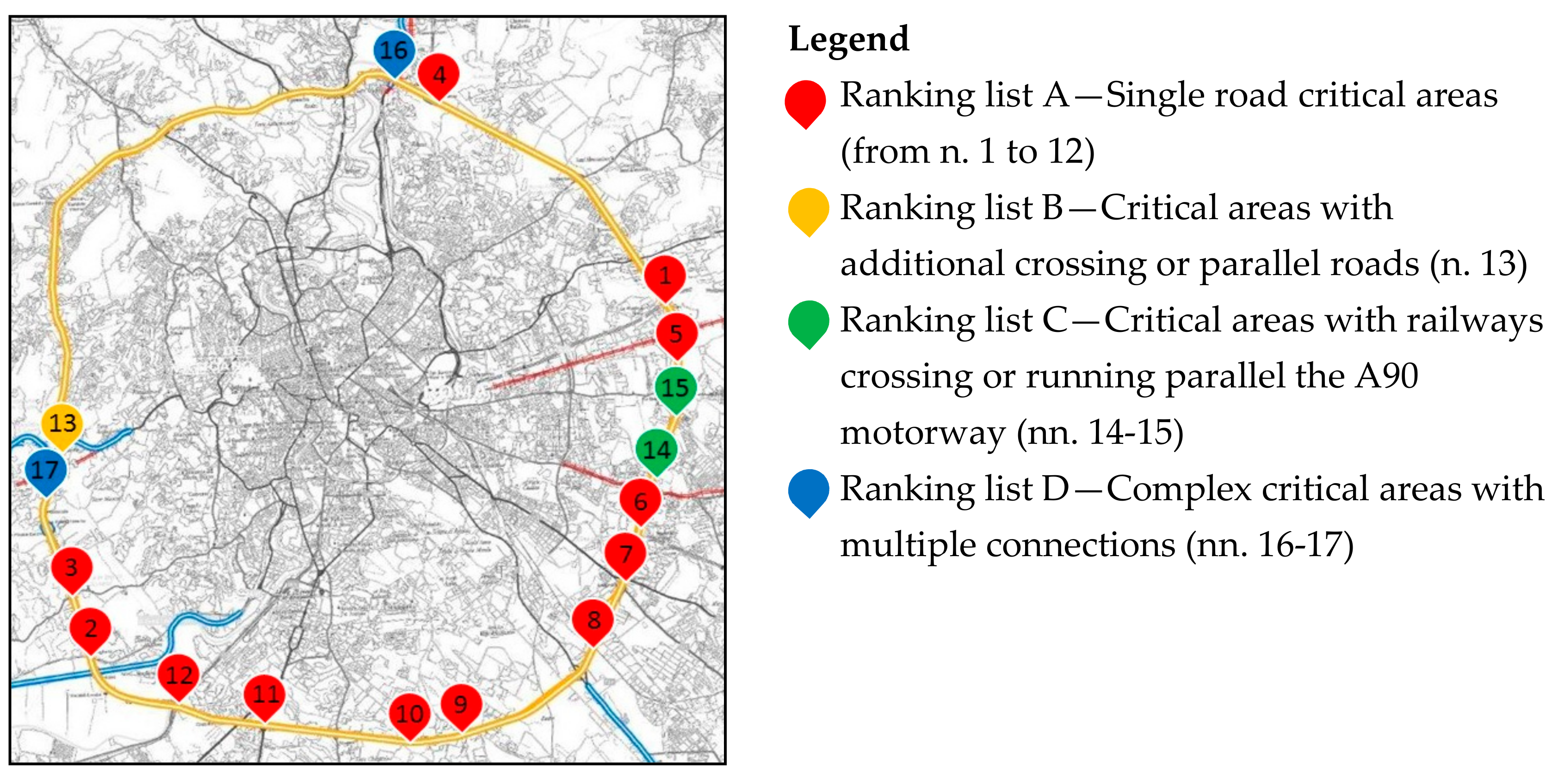
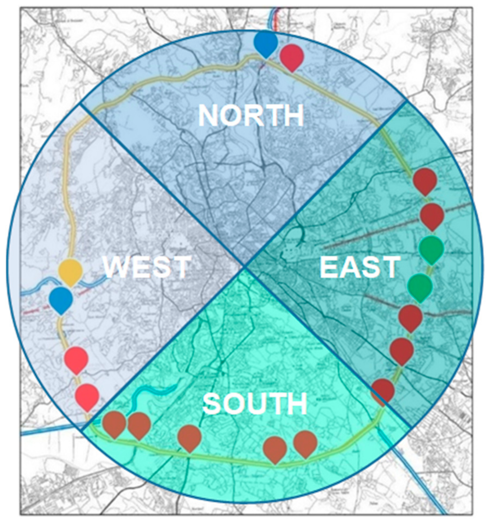
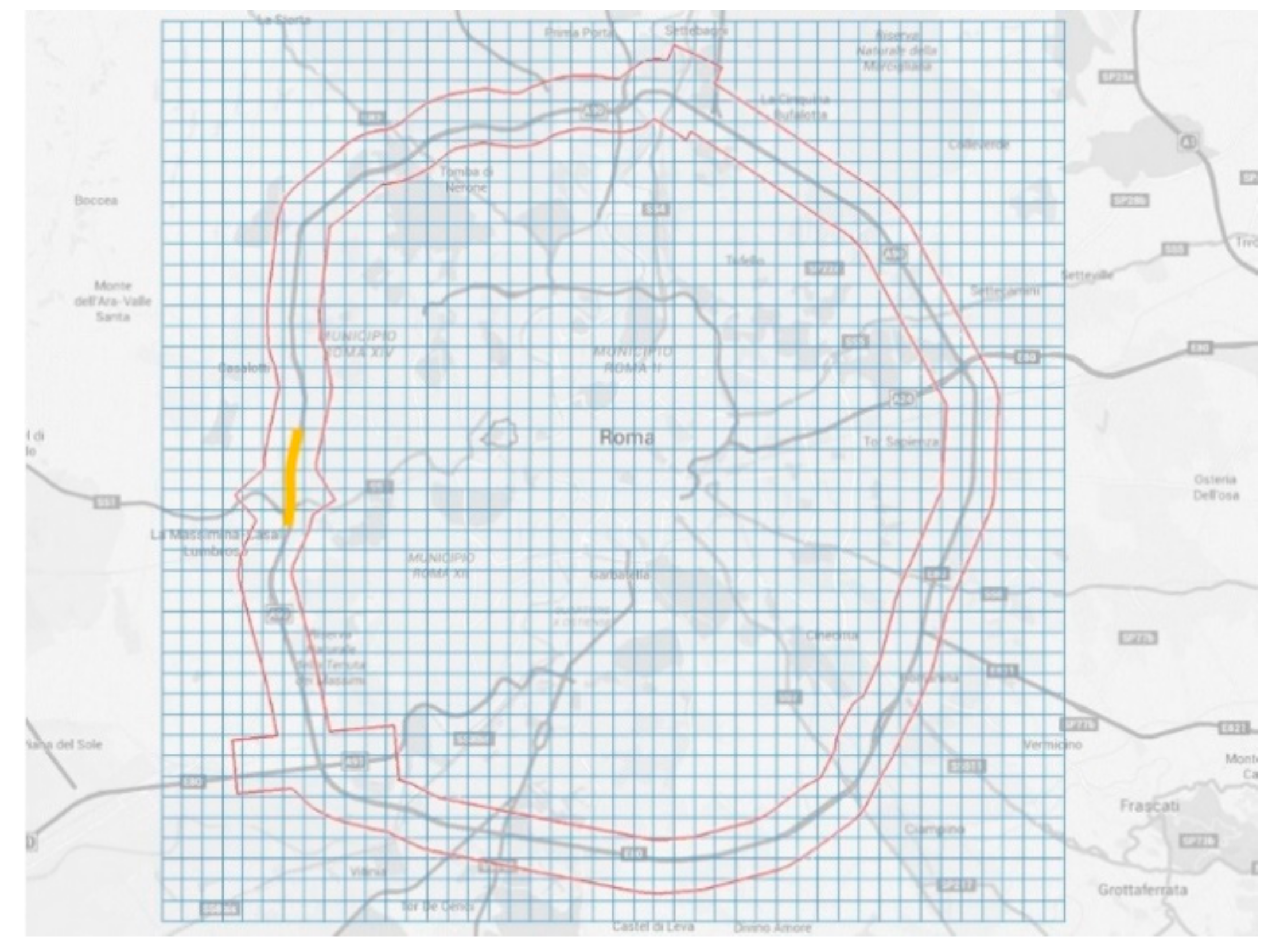
2.2. Pilot Area Selection
- Single road (A90 Motorway).
- Additional crossing or parallel roads.
- Railway lines running parallel or crossing the A90 motorway.
- Complex scenario including multiple connections.
2.3. Design and Configuration of the System
2.3.1. Clustering Procedure to Reduce the Number of Elementary Noise Sources
- Δ(h)i,j is the hourly coefficient related to the i-th junction and the j-th hour;
- Lw(main axis)i,j is the hourly sound power level related to the i-th measurement position on the main road axis associated with the i-th junction and the j-th hour; and
- Lw(junction)i,j is the hourly sound power level related to the i-th junction and the j-th hour.
2.3.2. Evaluation of the Influence of Weather Conditions on Sound Propagation
- a map for totally favorable conditions;
- a map for totally homogeneous conditions; and
- four maps for favorable conditions in the main wind sectors.
2.4. Basic Noise Maps Preparation and Update
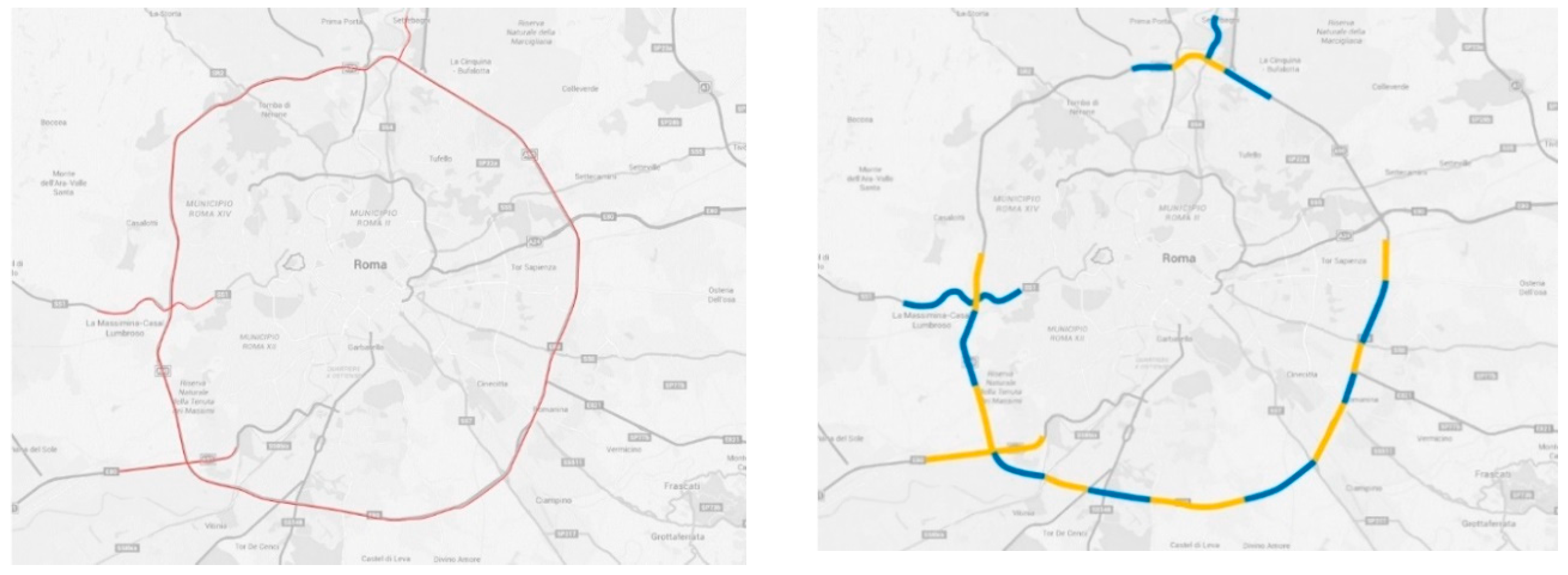
- To split the road network in stretches corresponding to the elementary noise sources (Figure 4);
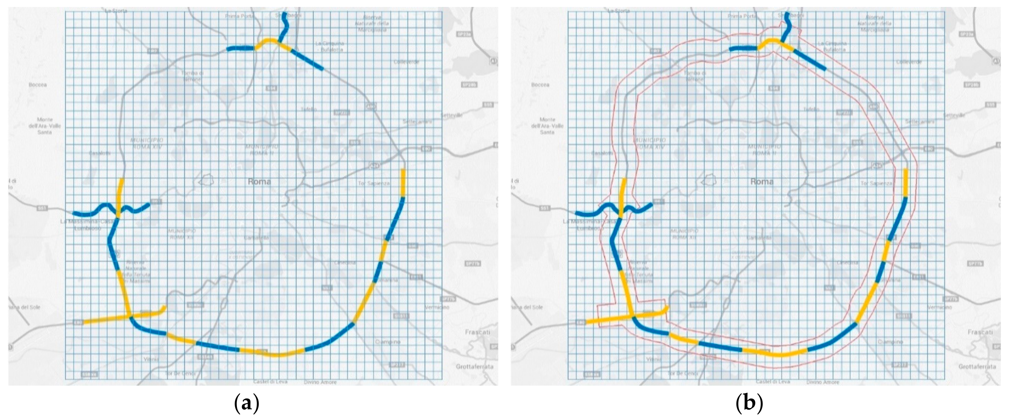
- To generate a unique grid for the whole pilot area, to avoid mismatching when summing up the different maps, and to prepare a unique calculation area corresponding to a buffer of 250 m each side around the ring road (Figure 5); and
- To turn on one elementary noise source at a time and calculate the whole set of basic noise maps in the whole calculation area (Figure 6).
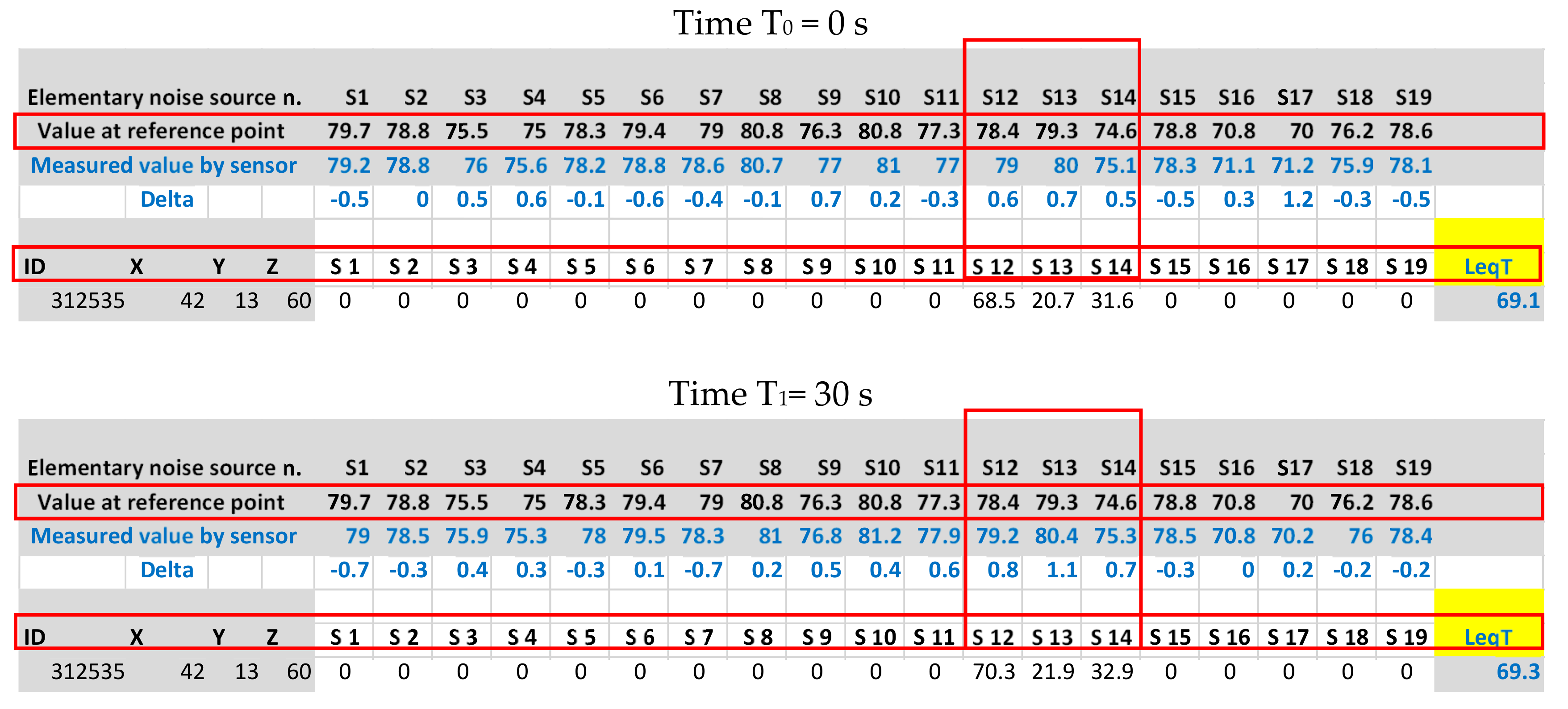
- is the final equivalent noise level associated with the j-th grid point;
- is the equivalent noise level related to the j-th grid point and the i-th elementary noise source; and
- is the number of elementary noise sources.
3. Measuring Campaign
3.1. Winter and Summer Campaign
3.2. Description of the Measurement Sites
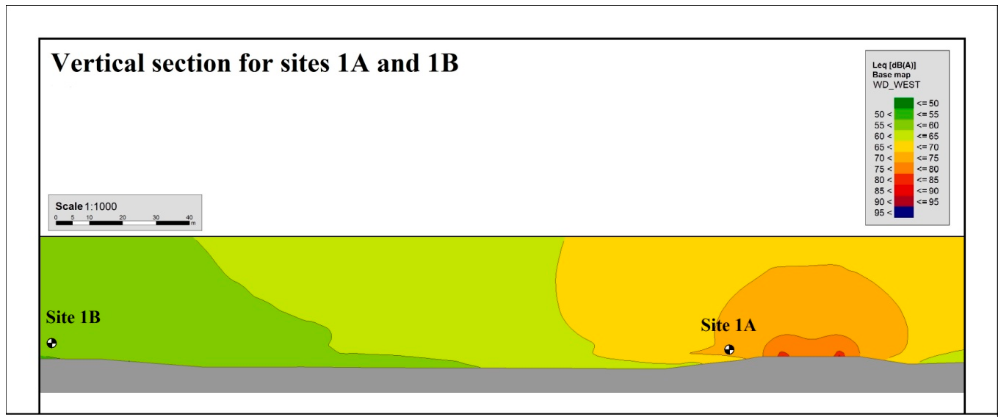
3.2.1. Site 1A-1B
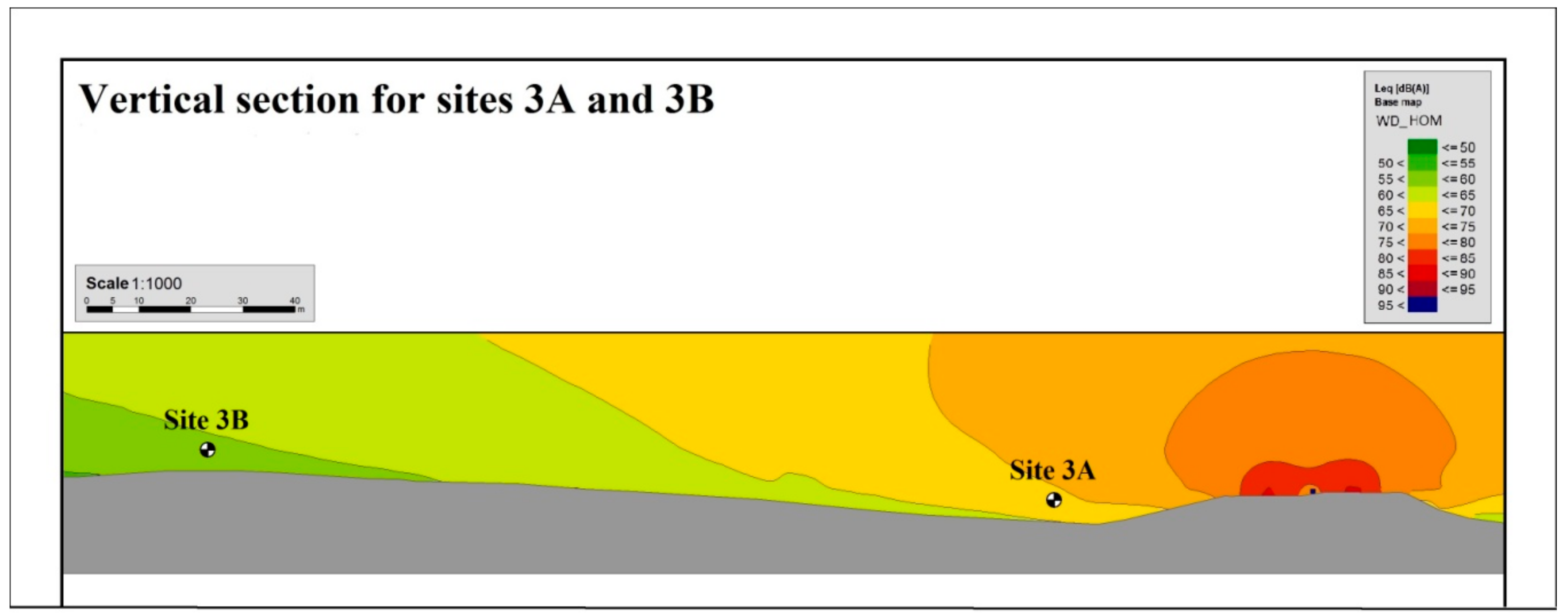
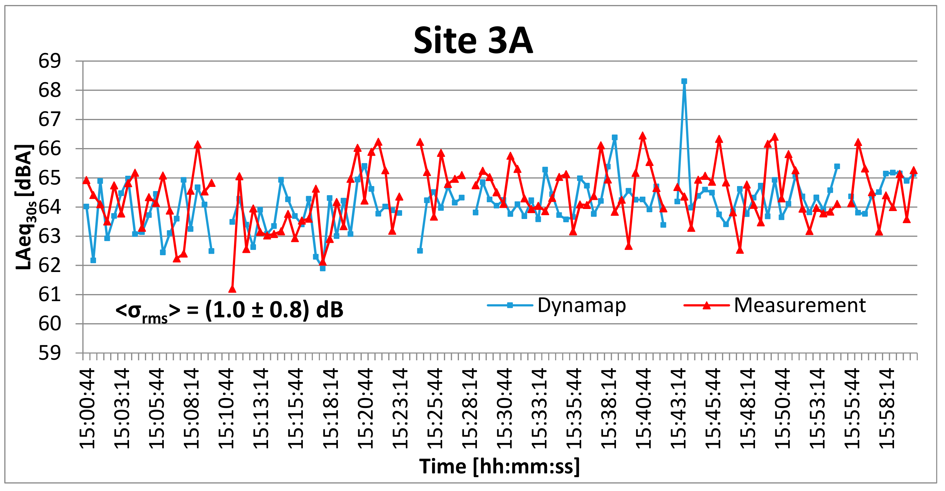
3.2.2. Sites 3A-3B
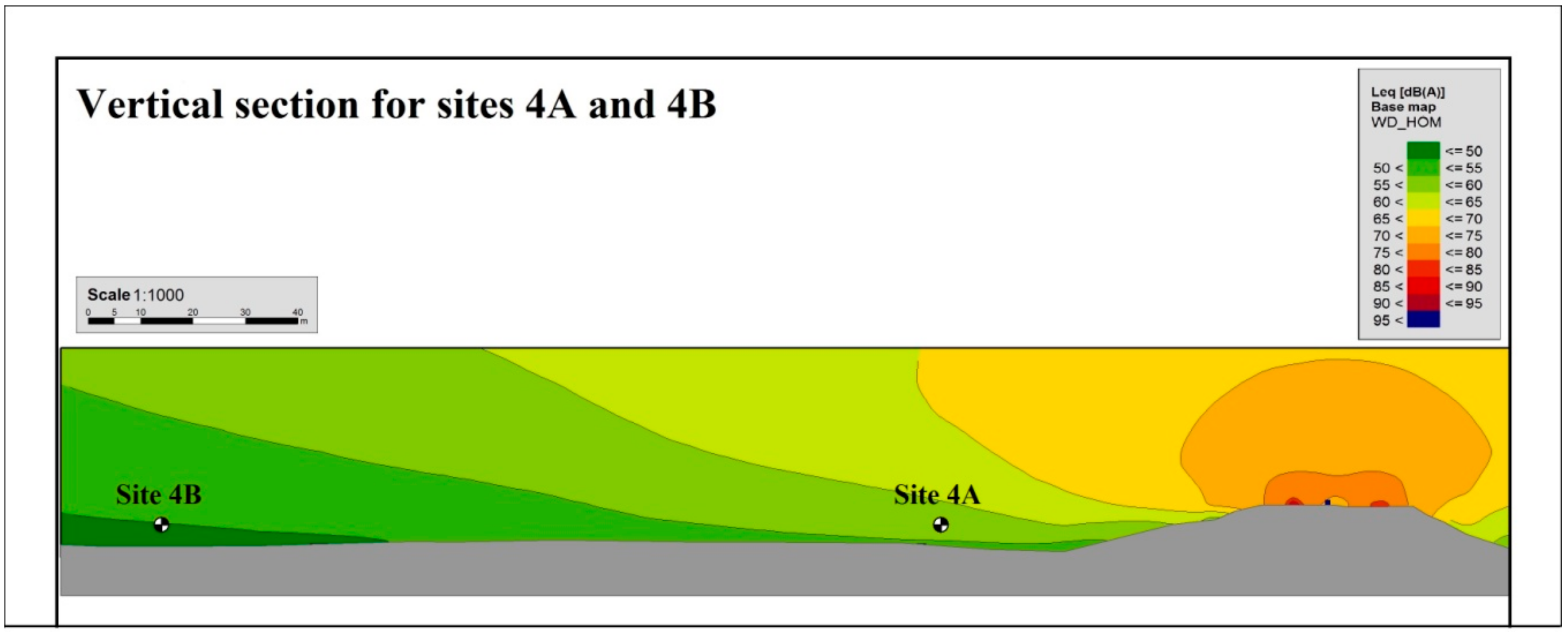
3.2.3. Sites 4A–4B
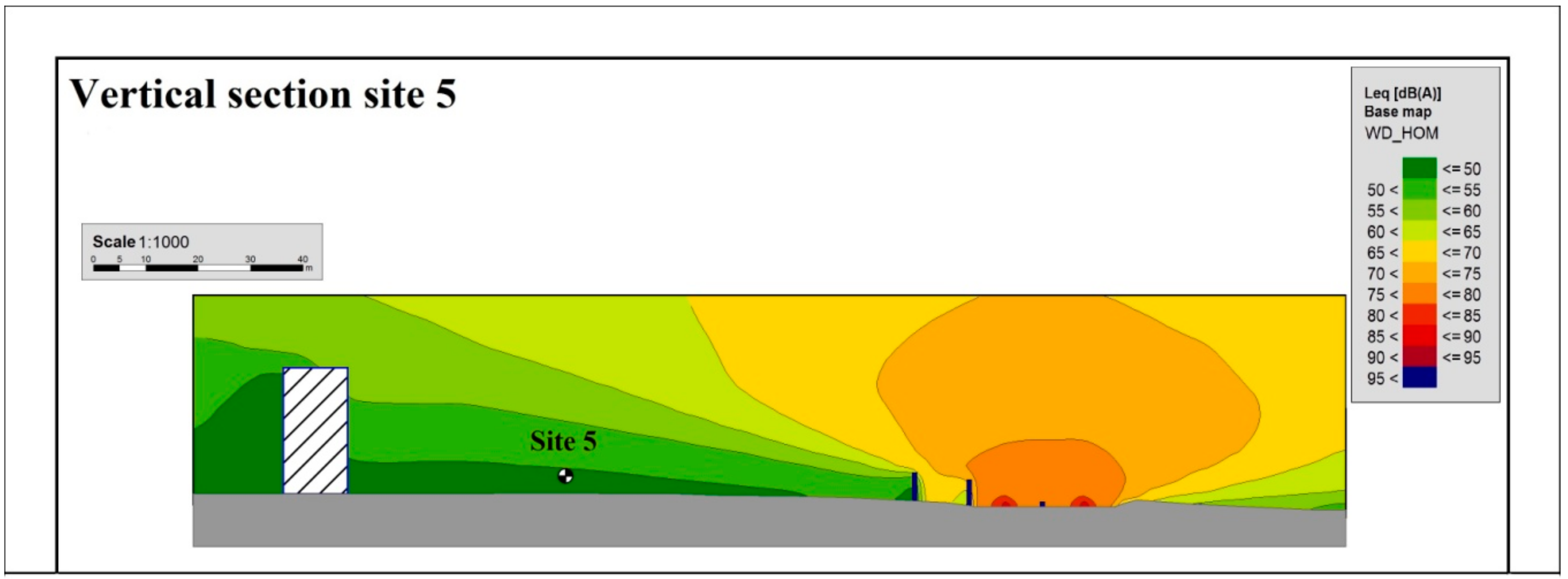
3.2.4. Site 5
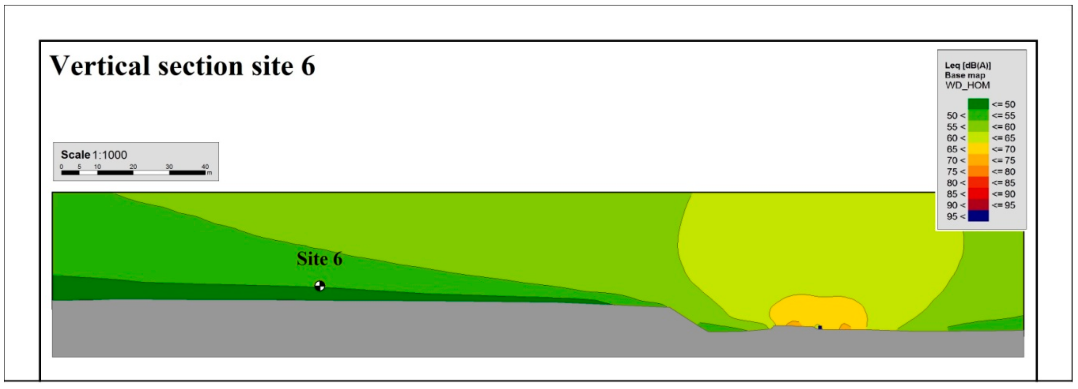
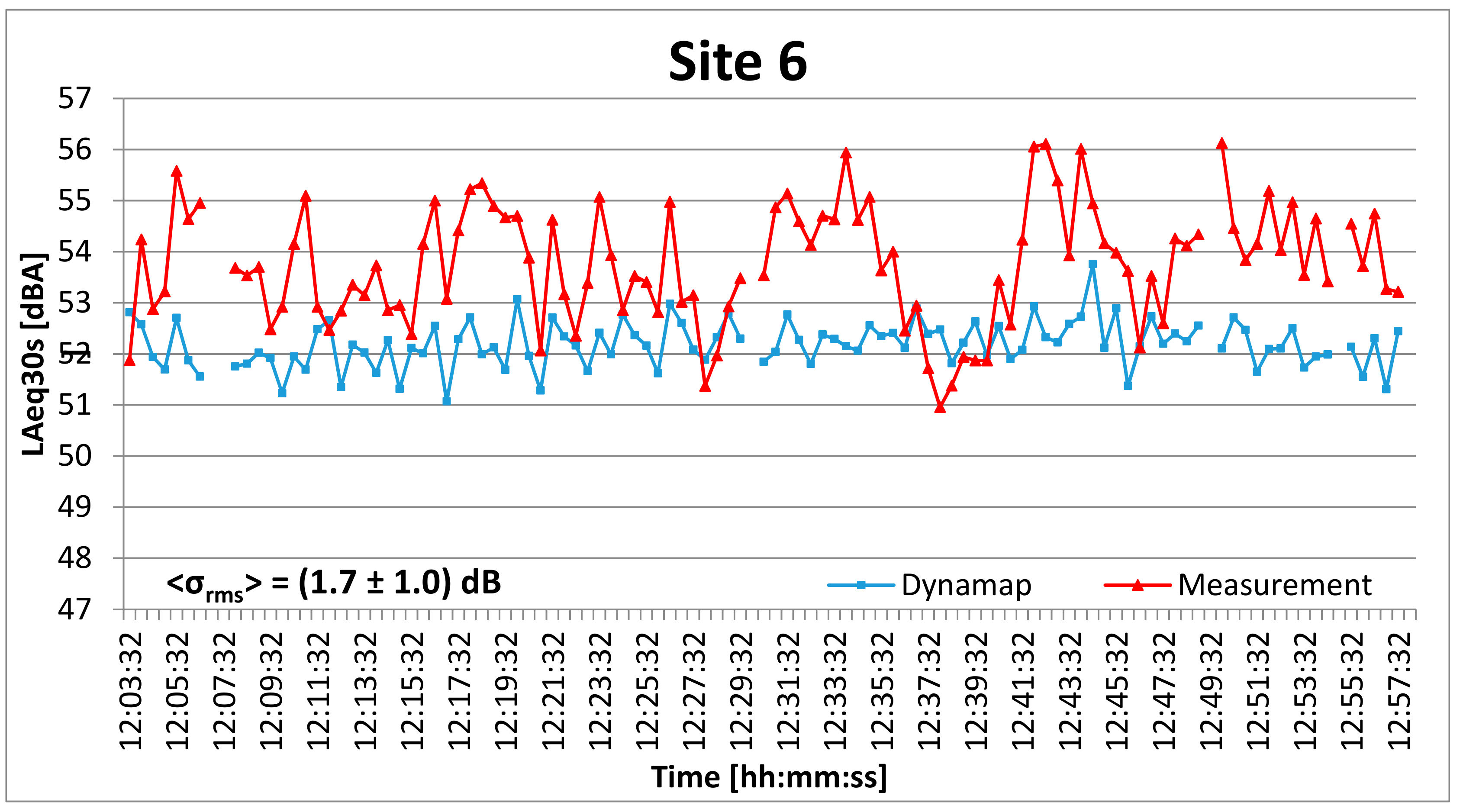
3.2.5. Site 6
3.3. DYNAMAP System Accuracy
4. Discussion
5. Conclusions
Author Contributions
Acknowledgments
Conflicts of Interest
References
- E. Union. Directive 2002/49/EC of the European Parliament and the Council of 25 June 2002 relating to the assessment and management of environmental noise. In Official Journal of the European Communities L 189/12; E. Union: Brussels, Belgium, 2002. [Google Scholar]
- E. Commission. Report From The Commission To The European Parliament And The Council On the Implementation of the Environmental Noise Directive in Accordance with Article 11 of Directive 2002/49/EC. COM/2017/0151; E. Commission: Brussels, Belgium, 2017. [Google Scholar]
- Licitra, G.; Ascari, E.; Fredianelli, L. Prioritizing Process in Action Plans: A Review of Approaches. Curr. Pollut. Rep. 2017, 109, 151–161. [Google Scholar] [CrossRef]
- Muzet, A. Environmental noise, sleep and health. Sleep Med. Rev. 2007, 11, 135–142. [Google Scholar] [CrossRef] [PubMed]
- De Kluizenaar, Y.; Janssen, S.A.; Van Lenthe, F.J.; Miedema, H.M.E.; MacKenbach, J.P. Long-term road traffic noise exposure is associated with an increase in morning tiredness. J. Acoust. Soc. Am. 2009, 126, 626–633. [Google Scholar] [CrossRef] [PubMed]
- Miedema, H.M.E.; Oudshoorn, C.G.M. Annoyance from Transportation Noise: Relationships with Exposure Metrics DNL and DENL and Their Confidence Intervals. Environ. Health Perspect. 2001, 109, 409–416. [Google Scholar] [CrossRef] [PubMed]
- Babisch, W.; Beule, B.; Schust, M.; Kersten, N.; Ising, H. Traffic Noise and Risk of Myocardial Infarction. Epidemiology 2005, 16, 33–40. [Google Scholar] [CrossRef] [PubMed]
- Babisch, W.; W, B. Road traffic noise and cardiovascular risk. Noise Health 2008, 10, 27. [Google Scholar] [CrossRef] [PubMed]
- Lercher, P.; Evans, G.W.; Meis, M. Ambient Noise and Cognitive Processes among Primary Schoolchildren. Environ. Behav. 2003, 35, 725–735. [Google Scholar] [CrossRef]
- Chetoni, M.; Ascari, E.; Bianco, F.; Fredianelli, L.; Licitra, G.; Cori, L. Global noise score indicator for classroom evaluation of acoustic performances in LIFE GIOCONDA project. Noise Mapp. 2016, 3, 157–171. [Google Scholar] [CrossRef]
- Van Kempen, E.; Babisch, W. The quantitative relationship between road traffic noise and hypertension: A meta-analysis. J. Hypertens. 2012, 30, 1075–1086. [Google Scholar] [CrossRef] [PubMed]
- Manvell, D.; Ballarin Marcos, L.; Stapelfeldt, H.; Sanz, R. SADMAM–Combining Measurements and Calculations to Map Noise in Madrid. In Proceedings of the Inter-Noise 2004, Prague, Czech Republic, 22–25 August 2004. [Google Scholar]
- Kozielecki, P.; Czyzewski, A. An application for vector-based dynamic noise maps generation. In Proceedings of the Joint Baltic-Nordic Acoustics Meeting 2008, Reykjavik, Iceland, 17–19 August 2008. [Google Scholar]
- De Coensel, B.; Sun, K.; Wei, W.; Van Renterghem, T.; Sineau, M.; Ribeiro, C.; Can, A.; Aumond, P.; Lavandier, C.; Botteldooren, D. Dynamic Noise Mapping Based on Fixed and Mobile Sound Measurements; EURONOISE 2015: Maastricht, France, 2015. [Google Scholar]
- Nencini, L.; Ascari, E.; Vinci, B. SENSEable Pisa: A wireless sensor network for real-time noise mapping. In Proceedings of the Euronoise 2012, Prague, Czech Republic, 10–14 June 2012. [Google Scholar]
- DYNAMAP. 2014. Available online: http://www.life-DYNAMAP.eu/ (accessed on 22 December 2017).
- Smiraglia, M.; Benocci, R.; Zambon, G.; Roman, H. Predicting hourly traffic noise from traffic flow rate model: Underlying concepts for the DYNAMAP project. Noise Mapp. 2016, 3, 130–139. [Google Scholar]
- Bellucci, P.; Peruzzi, L.; Zambon, G. LIFE DYNAMAP project: The case study of Rome. Appl. Acoust. 2017, 117, 193–206. [Google Scholar] [CrossRef]
- Benocci, R.; Angelini, F.; Bisceglie, A.; Zambon, G.; Bellucci, P.; Peruzzi, L.; Alsina-Pages, R.M.; Socoró, J.C.; Alías, F.; Orga, F. Initial verification of dynamic acoustic mapping along the motorway surrounding the city of Rome. In Proceedings of the INTER-NOISE and NOISE-CON Congress and Conference Proceedings, Chicago, IL, USA, 26–29 August 2018; The International Institute of Noise Control Engineering (I-INCE): Reston, VA, USA. [Google Scholar]
- Benocci, R.; Angelini, F.; Cambiaghi, M.; Bisceglie, A.; Roman, H.E.; Zambon, G.; Alsina-Pagés, R.M.; Socoró, J.C.; Alías, F.; Orga, F. Preliminary results of DYNAMAP noise mapping operations. In Proceedings of the INTER-NOISE and NOISE-CON Congress and Conference Proceedings, Chicago, IL, USA, 26–29 August 2018; The International Institute of Noise Control Engineering (I-INCE): Reston, VA, USA. [Google Scholar]
- Benocci, R.; Molteni, A.; Cambiaghi, M.; Angelini, F.; Roman, H.E.; Zambon, G. Traffic Noise Prediction Reliability of DYNAMAP Project. Appl. Acoust. (Accepted).
- Kephalopoulos, S.; Paviotti, M.; Anfosso Lédée, F. Common Noise Assessment Methods in Europe (CNOSSOS-EU); Publications Office of the European Union Report EUR 25379 EN (2002) 1-180; Publications Office of the European Union: Brussels, Belgium, 2002. [Google Scholar]
- Zambon, G.; Benocci, R.; Brambilla, G. Cluster categorization of urban roads to optimize their noise Monitoring. Environ. Monit. Assess. 2016, 188. [Google Scholar] [CrossRef] [PubMed]
- Zambon, G.; Benocci, R.; Bisceglie, A. Development of optimized algorithms for the classification of networks of road stretches into homogeneous clusters in urban areas. In Proceedings of the 22nd ICSV, Florence, Italy, 12–16 July 2015. [Google Scholar]
- Zambon, G.; Benocci, R.; Brambilla, G. Statistical Road Classification Applied to Stratified Spatial Sampling of Road Traffic Noise in Urban Areas. Int. J. Environ. Res. 2016, 10, 411–420. [Google Scholar]
- Orga, F.; Socoró, J.C.; Alsina-Pagès, R.M.; Zambon, G.; Benocci, R.; Bisceglie, A. Anomalous noise events considerations for the computation of road traffic noise levels: The DYNAMAP’ s Milan case study. In Proceedings of the 24th International Congress on Sound and Vibration, London, UK, 23–27 July 2017; pp. 23–27. [Google Scholar]
- Socoró, J.C.; Alías, F.; Alsina-Pagés, R.M. An anomalous noise events detector for dynamic road traffic noise mapping in real-life urban and suburban environments. Sensors 2017, 17, 2323. [Google Scholar] [CrossRef] [PubMed]
- Alías, F.; Socoró, J.C. Description of Anomalous Noise Events for Reliable Dynamic Traffic Noise Mapping in Real-Life Urban and Suburban Soundscapes. Appl. Sci. 2017, 7, 146. [Google Scholar] [CrossRef]
- Alsina-Pagés, R.M.; Orga, F.; Alías, F.; Socoró, J.C.; Benocci, R.; Zambon, G. Removing Anomalous Events for Reliable Road Traffic Noise Maps Generation: From Manual to Automatic Approaches. Appl. Acoust. 2019, 151, 183–192. [Google Scholar] [CrossRef]


| ID | LAT | LONG | NS1 dB(A) | NS2 dB(A) | NS3 dB(A) | … | NSN dB(A) | Leq T dB(A) |
|---|---|---|---|---|---|---|---|---|
| 0001 | X0001 | Y0001 | L11 | L12 | L13 | … | L1N | LeqR1 |
| 0002 | X0002 | Y0002 | L21 | L22 | L23 | … | L2N | LeqR2 |
| … | … | … | … | … | … | … | … | … |
| … | … | … | … | … | … | … | … | … |
| … | … | … | … | … | … | … | … | … |
| … | … | … | … | … | … | … | … | … |
| 9999 | X9999 | Y9999 | L99991 | L9992 | L99993 | … | L9999N | LeqR9999 |
| Site | Latitude | Longitude | Distance from A90 [m] |
|---|---|---|---|
| 1A | 41°56′15.4″ N | 12°35′53.6″ E | 15 |
| 1B | 41°56′16.2″ N | 12°36′02.2″ E | 195 |
| 3A | 41°47′41.1″ N | 12°30′25.2″ E | 25 |
| 3B | 41°47′46.3″ N | 12°30′28.0″ E | 190 |
| 4A | 41°57′39.6″ N | 12°34′35.8″ E | 55 |
| 4B | 41°57′43.8″ N | 12°34′36.6″ E | 180 |
| 5 | 41°52′24.6″ N | 12°36′17.2″ E | 90 |
| 6 | 41°50′47.1″ N | 12°22′59.0″ E | 100 |
| Site | <σrms> [dB] |
|---|---|
| 1a | 1.8 ± 0.7 |
| 1b | 1.0 ± 0.8 |
| 3a | 1.0 ± 0.8 |
| 3b | 1.5 ± 1.2 |
| 4a | 1.7 ± 1.1 |
| 4b | 1.8 ± 1.2 |
| 5 | 1.5 ± 0.9 |
| 6 | 1.7 ± 1.0 |
© 2019 by the authors. Licensee MDPI, Basel, Switzerland. This article is an open access article distributed under the terms and conditions of the Creative Commons Attribution (CC BY) license (http://creativecommons.org/licenses/by/4.0/).
Share and Cite
Benocci, R.; Bellucci, P.; Peruzzi, L.; Bisceglie, A.; Angelini, F.; Confalonieri, C.; Zambon, G. Dynamic Noise Mapping in the Suburban Area of Rome (Italy). Environments 2019, 6, 79. https://0-doi-org.brum.beds.ac.uk/10.3390/environments6070079
Benocci R, Bellucci P, Peruzzi L, Bisceglie A, Angelini F, Confalonieri C, Zambon G. Dynamic Noise Mapping in the Suburban Area of Rome (Italy). Environments. 2019; 6(7):79. https://0-doi-org.brum.beds.ac.uk/10.3390/environments6070079
Chicago/Turabian StyleBenocci, Roberto, Patrizia Bellucci, Laura Peruzzi, Alessandro Bisceglie, Fabio Angelini, Chiara Confalonieri, and Giovanni Zambon. 2019. "Dynamic Noise Mapping in the Suburban Area of Rome (Italy)" Environments 6, no. 7: 79. https://0-doi-org.brum.beds.ac.uk/10.3390/environments6070079