Article

Spatiotemporal Variability in Phytoplankton Bloom Phenology in Eastern Canadian Lakes Related to Physiographic, Morphologic, and Climatic Drivers

by
Claudie Ratté-Fortin
1,2,
Karem Chokmani
1,2,* and
Isabelle Laurion
1,2
1
Institut national de la recherche scientifique, Centre Eau Terre Environnement, 490 Rue de la Couronne, Quebec City, QC G1K 9A9, Canada
2
Interuniversity Research Group in Limnology, University of Montreal, C.P. 6128, Succ. Centre-Ville, Montreal, QC H3C 3J7, Canada
*
Author to whom correspondence should be addressed.
Submission received: 31 July 2020 / Revised: 17 September 2020 / Accepted: 21 September 2020 / Published: 27 September 2020

Abstract

:
Phytoplankton bloom monitoring in freshwaters is a challenging task, particularly when biomass is dominated by buoyant cyanobacterial communities that present complex spatiotemporal patterns. Increases in bloom frequency or intensity and their earlier onset in spring were shown to be linked to multiple anthropogenic disturbances, including climate change. The aim of the present study was to describe the phenology of phytoplankton blooms and its potential link with morphological, physiographic, anthropogenic, and climatic characteristics of the lakes and their watershed. The spatiotemporal dynamics of near-surface blooms were studied on 580 lakes in southern Quebec (Eastern Canada) over a 17-year period by analyzing chlorophyll-a concentrations gathered from MODIS (Moderate Resolution Imaging Spectroradiometer) satellite images. Results show a significant increase by 23% in bloom frequency across all studied lakes between 2000 and 2016. The first blooms of the year appeared increasingly early over this period but only by 3 days (median date changing from 6 June to 3 June). Results also indicate that high biomass values are often reached, but the problem is seldom extended to the entire lake surface. The canonical correlation analysis between phenological variables and environmental variables shows that higher frequency and intensity of phytoplankton blooms and earlier onset date occurred for smaller watersheds and higher degree-days, lake surface area, and proportion of urban zones. This study provides a regional picture of lake trophic state over a wide variety of lacustrine environments in Quebec, a detailed phenology allowing to go beyond local biomass assessments, and the first steps on the development of an approach exploiting regional trends for local pattern assessments.

1. Introduction

The marked increase in freshwater algal blooms is of major interest to governments and public health agencies responsible for maintaining the ecological services provided by these systems. Cyanobacteria threaten the ecological integrity of some of the world’s most important lake environments, including Lake Erie [1], Lake Ontario [2], Lake Taihu [3], Lake Okeechobee [4], and Lake Victoria [5]. Their increasing frequency and sustained presence affect the structure and functioning of aquatic food webs [6], limit recreational activities [7], and threaten drinking water sources [8]. Monitoring phytoplankton blooms remains difficult and onerous, particularly because their spatial and temporal distribution is highly variable when dominated by buoyant cyanobacteria [9,10].
Several models have been developed to describe the mechanisms involved in bloom onset, development, maintenance and decline, including ecological models based on phytoplankton growth response mechanisms [11,12,13,14], and hydrological models involving nutrient production, transport, and accumulation [15]. Other studies have focused on the relationships between the development of phytoplankton blooms and the environmental conditions prevailing in water bodies or watersheds [16,17,18]. Among others, Hu et al. [19] and Liu et al. [20] have demonstrated the impact of climatic variables (air temperature, relative humidity, wind speed and direction) on the development of cyanobacterial blooms. Several other studies have shown relations between chlorophyll a concentration (Chl-a) and key physicochemical factors associated with phytoplankton development [21,22]. The main disruptive elements identified are phosphorus [23,24,25] and nitrogen when phosphorus is no longer limiting [23,26]. The N:P ratio is also used as an indicator of the occurrence of cyanobacterial [27,28,29] and other phytoplankton blooms [30,31]. Water temperature and light availability has also been shown to play a major role in bloom development [32] in a way that is specific to each species [33].
These models, most being empirical, allowed to target disruptive elements and characterize their effect on spatiotemporal patterns of phytoplankton blooms. It remains fairly difficult, however, to identify all disruptive elements acting upon a given water body or on an annual basis. In order to develop solutions for the protection or restoration of water bodies, it is necessary to identify major sources of disruption among the multiple anthropogenic disturbances concurrently taking place [34,35] and to define their specific effect on the frequency, intensity, and duration of blooms. The supply of local or diffuse sources of nutrients to a water body is related to the physiography of its watershed. For example, the nutrient storage capacity is influenced by the size of the watershed; the type of soil affects runoff and infiltration rates; and the shape and topography of the watershed act upon peak flows and soil erosion [36]. Moreover, climatic variables play an undeniable role in the development of blooms, including air temperature, precipitation, wind, and hours of sunlight [37,38]. Bloom intensity and frequency were shown to increase in response to climate change [38,39,40,41,42,43] and to occur earlier in the spring [44,45].
This study is part of a project aiming to estimate lake predisposition to phytoplankton blooms based on the environmental conditions prevailing on its watershed. The ultimate goal is to provide a tool to project future scenarios of bloom phenology in response to climate change and anthropogenic developments, or to test the efficiency of mitigating approaches. To do so, the first step was to set up a database of near-surface phytoplankton bloom phenological characteristics (frequency, intensity, surface area, onset date, end date, and duration) between 2000 and 2016 from 580 lakes in Quebec, Canada, using satellite images from the MODIS (Moderate Resolution Imaging Spectroradiometer) sensor. This database was then used to target key environmental variables involved in defining this phenology, including the morphological, physiographic, anthropogenic, and climatic characteristics of the lakes and their watershed, through a canonical correlation analysis (CCA). We further illustrate the results for two lakes particularly affected by blooms, the Missisquoi Bay of Lake Champlain and Lake Brome. A frequency analysis model linking the phenological characteristics of phytoplankton blooms with the environmental conditions at the regional scale will later be presented in a sister paper.

2. Materials and Methods

The lakes studied are located in the province of Quebec, Canada, between 44° N and 50° N and 67° W and 80° W, covering an area of approximately 600,000 km2 (Figure 1). The spatial distribution of the lakes was homogeneous throughout the study area, as verified by the Ripley’s index suggesting a regular pattern [46]. This territory mainly consists of podzolic soils and is characterized by a humid continental climate in the south and a subarctic climate in the north. Industrial and agricultural developments are widespread in the southwestern area of the territory, while the northern part is much less developed.
A database of historical Chl-a concentrations was generated from satellite data acquired by the MODIS sensor (bands 1–7) located on NASA’s Earth Observation System Terra platform, at a temporal frequency of 1 day. The spatial resolution of the bands 3–7 was refined from 500 m to 250 m using a spatial resolution downscaling approach developed by Trishchenko et al. [47]. This approach was validated using high resolution spatial data (Landsat ETM+ at 30 m) demonstrating that the radiometric properties of the downscaled bands were not altered. Image pre-treatment, including downscaling, projection, and atmospheric correction, was achieved using an automated procedure developed by the Canadian Center for Remote Sensing [47]. An estimation algorithm for Chl-a concentrations based on ensemble methods [48] was then applied to all MODIS images extracted. This algorithm was specifically developed for inland waters and performed well on databases with Chl-a ranging from low to high concentrations (see Appendix A). In order to reduce the uncertainty related to the heterogeneous elements on lakeshores (e.g., build environments, lake bottom), mixed pixels (water-land boundary) were removed over a 250 m band by applying a ground mask. This procedure generated a composite image formed by the minima of reflectance in the near infrared on images captured between May and October of 2000 to 2016. This avoids interference by macrophytes, since the reflectance of water pixels with phytoplankton will be inferior to that of the pixels occupied by macrophytes, which are more permanent elements in the littoral zone during the open-water season. In order to have enough pixels to adequately represent each water body, only lakes with a minimum area of 3.5 km2 were considered for this study. Areas affected by haze or cloud cover were then removed using a cloud mask [49] specifically developed for inland waters (lakes, rivers, estuaries). Only lakes having less than 25% cloud cover for a given image were selected. Overall, Chl-a concentrations were extracted from 580 lakes in southern Quebec between May and October of the years 2000 to 2016, for a total of 1572 images.
An operational biomass threshold of 10 µg Chl-a L−1 was chosen to define the onset of a bloom and characterize its phenology on the studied lakes. It corresponds to the lower end of the eutrophic lake class (8–25 µg L−1) and to the decision threshold for recreational water level 1 as established by the World Health Organization [50] and the government of Quebec [51]. When level 1 threshold is exceeded and biomass becomes dominated by cyanobacteria, it is considered a risk of minor health effects (irritation and allergies). This threshold is already used by watershed-based organizations, water management officers and municipalities.
For each studied year, phenological variables were established as follows: (1) the frequency, which is the number of days when Chl-a concentrations remained above the threshold, (2) the intensity, which is the maximum concentration of Chl-a detected during a bloom, (3) the relative area, which is the maximum area occupied by a bloom normalized by the lake area, (4) the onset date, and (5) the end date, which are the first and last days of the year when a bloom is detected, and (6) the duration, which is the number of days between the onset date and the end date. Determination of the end date and duration of blooms is challenging because the studied region is frequently covered by clouds during the fall, significantly reducing the number of MODIS images available for this period. This is especially true during the month of October, for which there was on average half as many MODIS images without full cloud cover than for months between May and September. Therefore, end date and duration were discarded from the study. The retained variables describe what can be considered as an annual-based phenology, compiling days with less than 25% cloud cover and for which remotely-sensed Chl-a was above the established threshold, for any given pixel.
A geo-referenced database of the morphological, physiographic, and climatic characteristics of the watershed of each studied lake was established. The boundaries and morphological descriptors of the watersheds (area, slope) were calculated from the Canadian Digital Elevation Model [52] with a spatial resolution of approximately 30 m. Climate data from North American Regional Reanalyses [53], with a spatial resolution of approximately 32 km, were used. The cumulative degree-days (°C day) were calculated by summing the recorded degrees (°C) each day above 20 °C, a value that has been considered a threshold for cyanobacterial growth [54,55]. Even though the remote sensing approach used here is not specific to cyanobacterial biomass, this climate proxy is considered valid. Land use data (at 40 m spatial resolution) and agricultural and ecumene data (at 25 m spatial resolution) were provided by Natural Resources Canada [56,57]. The environmental indicators were considered stationary over the period 2000–2016. A total of 27 environmental variables were extracted for each lake and their watershed. The variables with the highest correlation to phytoplankton bloom phenology were selected (see Section 3.2) for statistical analysis (Table 1).
The spatial variability in phenological data is presented according to the latitude or longitude of the concerned lakes, and was statistically tested using the Kruskal and Wallis [58] test by randomly generating a subsample of lakes (by longitude or latitude) to ensure the independence of variables (runs test [59]). Temporal trend tests were conducted on median and annual extreme values (5th or 95th percentile; normality test [60]). Given the size and diversity of the generated data sets and the complexity of the interactions governing bloom phenology, analyses were carried out using canonical methods. The aim was to explore all possible correlations between phenological and environmental variables without using one group of variables to justify the other. The canonical correlation analysis (CCA) allows to simultaneously analyze two groups of variables by quantifying their association. The objects (lakes) under study are described by two sets of quantitative descriptors: the first set X1 of p phenological descriptors, and the second set X2 of q environmental descriptors. Linear combinations Ui = AiX1 and Vi = BiX2 (Ai and Bi are parameters; i = 1, …, K) of each set of descriptors are calculated in such a way that the canonical correlation between Ui and Vi is the highest possible. The first pair of canonical variables i   =   1 is the pair of linear combinations U 1 and V 1 , which maximizes the equation’s correlation. The second pair of canonical variables i = 2 is the pair of linear combinations U2 and V2 which maximizes the correlation of this equation and which is not correlated with the first pair of canonical variables. This process is repeated until K pairs of canonical variables are obtained, such as K = min (p, q). The significance of canonical correlations was tested using Bartlett’s approximate chi-squared statistic [61,62]. The interpretation of canonical variables was based on the identification of: (1) standardized canonical coefficients A i and B i , (2) structure coefficients R ( U i , X 1 p ) and R ( V i ,   X 2 q ) , and (3) canonical communality coefficients h 2 . The contribution of original variables to a given canonical variables was estimated from standardized canonical coefficients A i and B i . These weights are generated to maximize the canonical correlation R i , and are thus similar to the weights of a regression. Standardized coefficients assess the importance of one variable in relation to the others, and thus reflect their contribution to the canonical correlation. Structure coefficients were also calculated to evaluate the importance of a given unrelated variable. These coefficients correspond to the correlations between the original variables and the canonical variables R . The correlations (when squared) indicate the proportion of variance linearly shared by a given original variable with the canonical variable. Note that R correlations are not affected by the standardization of the original variables. Finally, the canonical communality coefficients ( h 2 ) correspond to the sum of the squared R of all the canonical variables interpreted in the analysis. They provide information on the proportion of variance of a variable that is explained by the set of canonical variables used in the analysis. Variables with low values (<45%) are generally omitted from the analysis [63]. Although multicolinearity between variables does not present any analytical difficulties when using a CCA, it can complicate the interpretation of the results by blurring the origin of the observed effects [64]. The combined use of standardized and structure coefficients is therefore recommended since the latter are not affected by multicollinearity, and informs us on the potential contribution of the observed variables to the development of canonical variables [65]. Satellite data treatment and statistical analyses were computed using Matlab software (R2018b).

3. Results

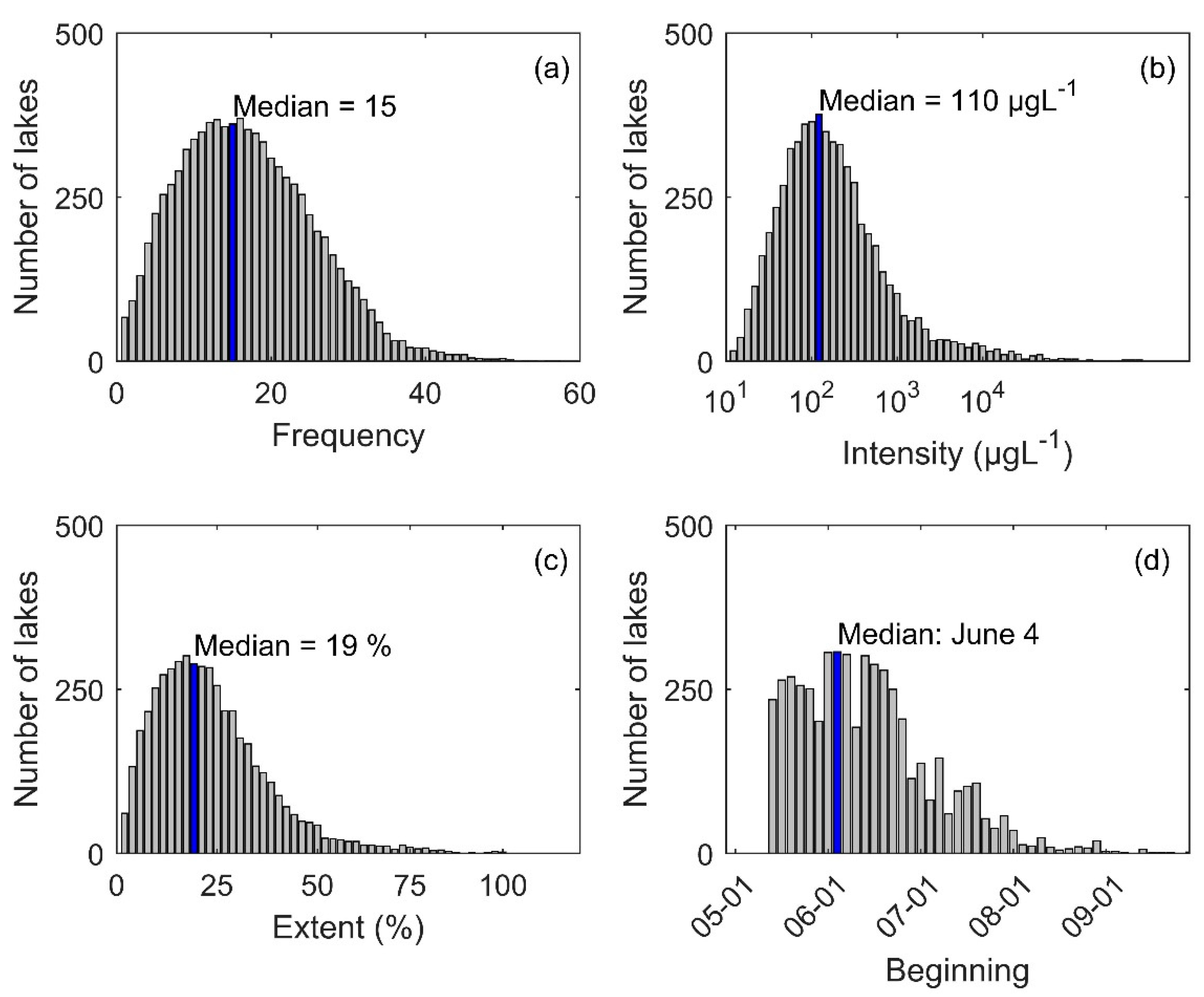
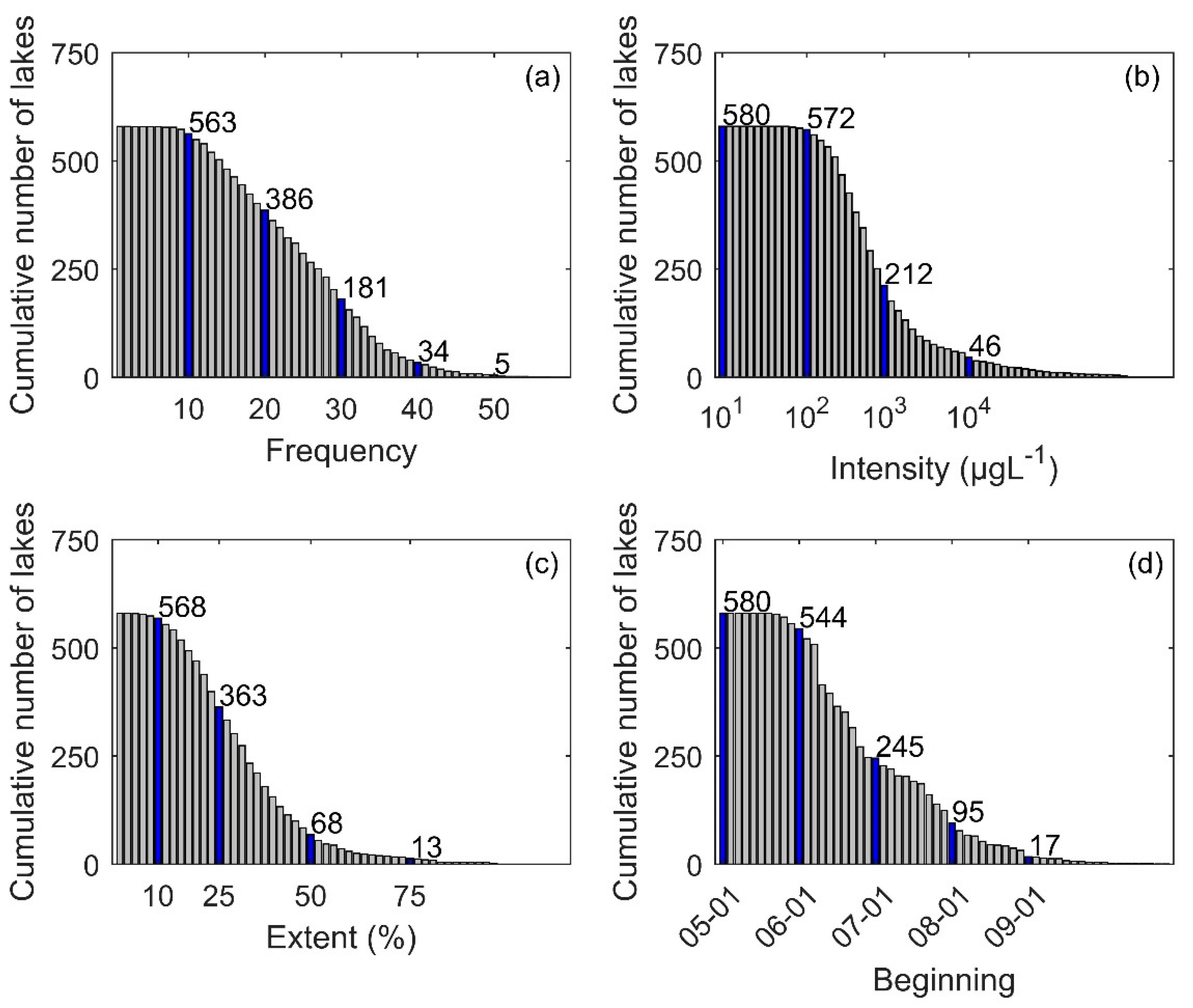
3.1. Descriptive Analysis of Bloom Events

Figure 2 shows the distribution histograms of the phenological variables. The median frequency of blooms was 15 days per year for all the lakes and years considered (Figure 2a). Among all lakes, the median intensity (maximum Chl-a concentration for a given lake) was 110   μ g   L 1 ( 2160   μ g   L 1 for the 95th percentile; Figure 2b), and the median surface area (maximum relative surface area) was 19 % (Figure 2c). The distribution shape is similar across phenological variables and shows a left-sided asymmetry. However, the shape of the onset date distribution is left truncated (Figure 2d). This is because mapping of Chl-a using satellite imagery does not begin until mid-May of each year to ensure that the lakes further north are completely thawed out. Thus, the median date of the first algal bloom is 4 June on the available dataset. This date could be slightly earlier with a more complete distribution of this phenological variable (i.e., including lakes that thawed before 15 May).
Figure 3 presents the complementary cumulated histogram of the phenological variables. For instance, more than 180 lakes showed 30 days during which Chl-a concentrations were above the threshold of 10 µg L−1 (for any specific year between 2000 and 2016), while only five lakes showed at least 50 days exceeding this threshold (Figure 3a): Missisquoi Bay (2012), Lake Saint-Louis (2005, 2012, 2013), Lake Des-Deux-Montagnes (2005, 2012), Lake Saint-Pierre (2013), and Lake Saint-François (2012). The last four water bodies are fluvial lakes generally presenting low intensities (median values between 12 and 15 µg Chla L−1). Five hundred seventy-two lakes also showed Chl-a concentrations of 100 µg L−1 or more at least once between 2000 and 2016 (Figure 3b). However, the number of lakes with such high concentrations over a significant portion of the surface area (above 50% of the lake area) dropped to 54 (not shown; Figure 3 rather presents the extent for biomasses > 10 µg L−1). On the other hand, only 13 lakes had experienced an extended bloom (covering at least 75% of their area) over the period 2000–2016 (Figure 3c), including Lake Brome and Missisquoi Bay.

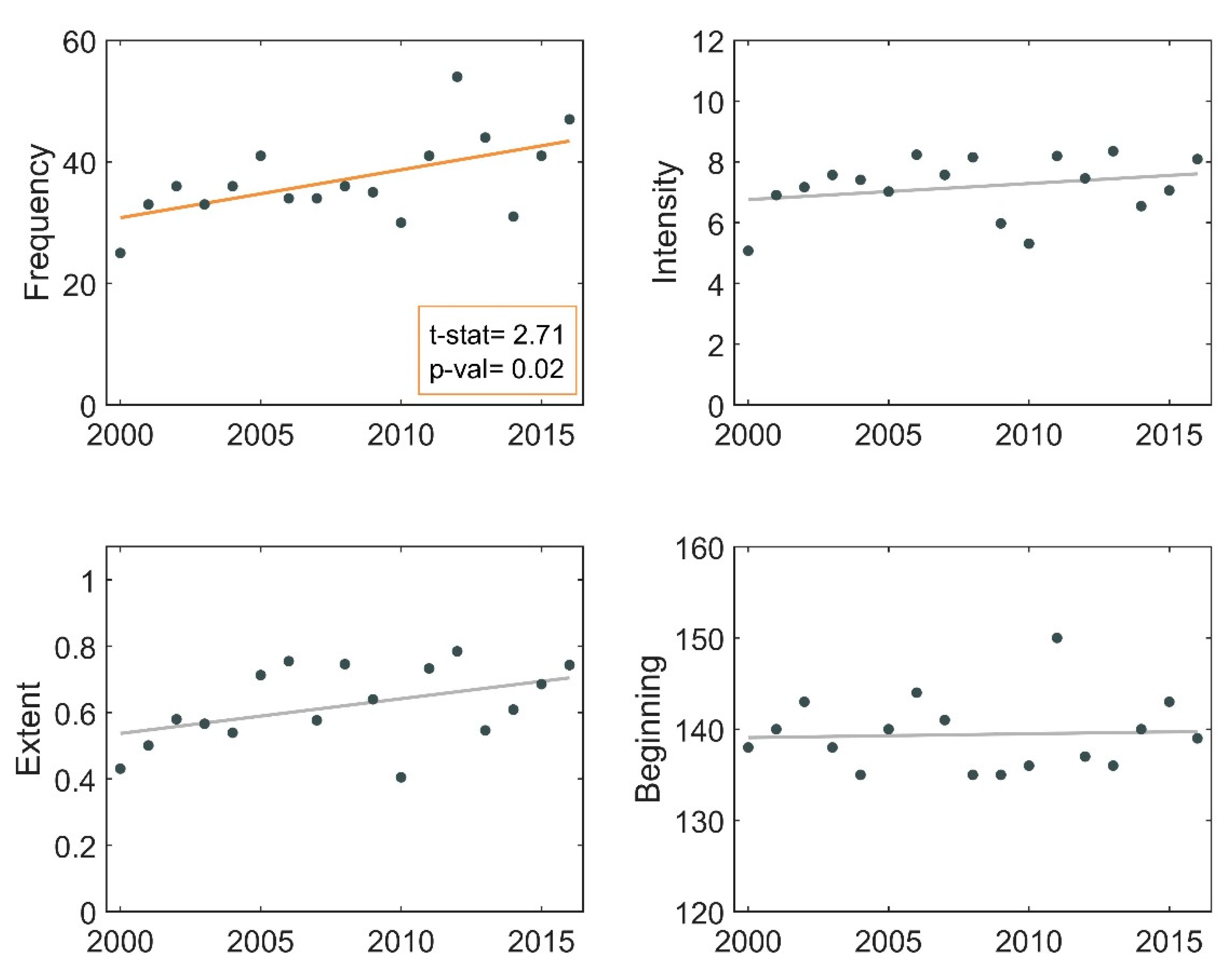
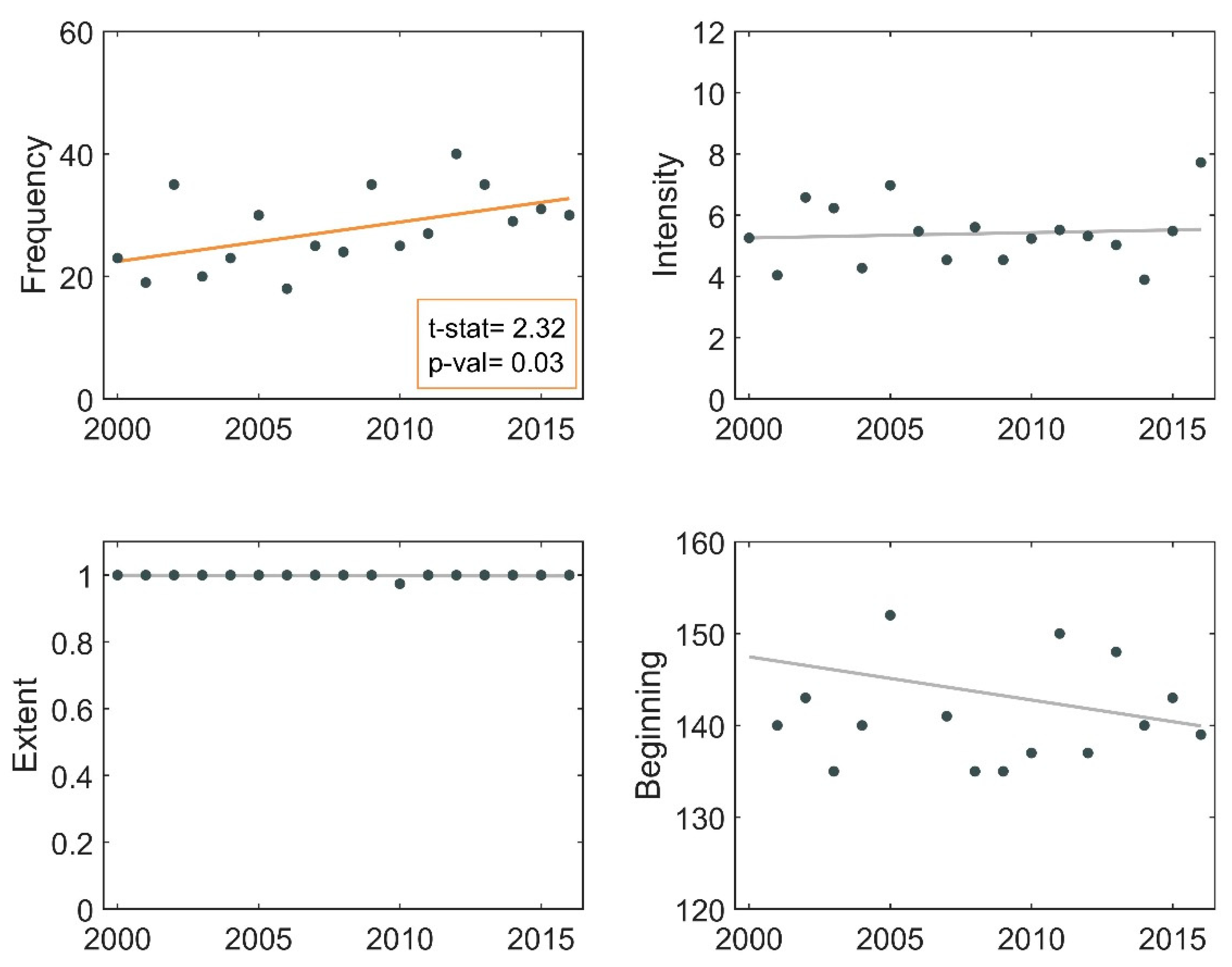
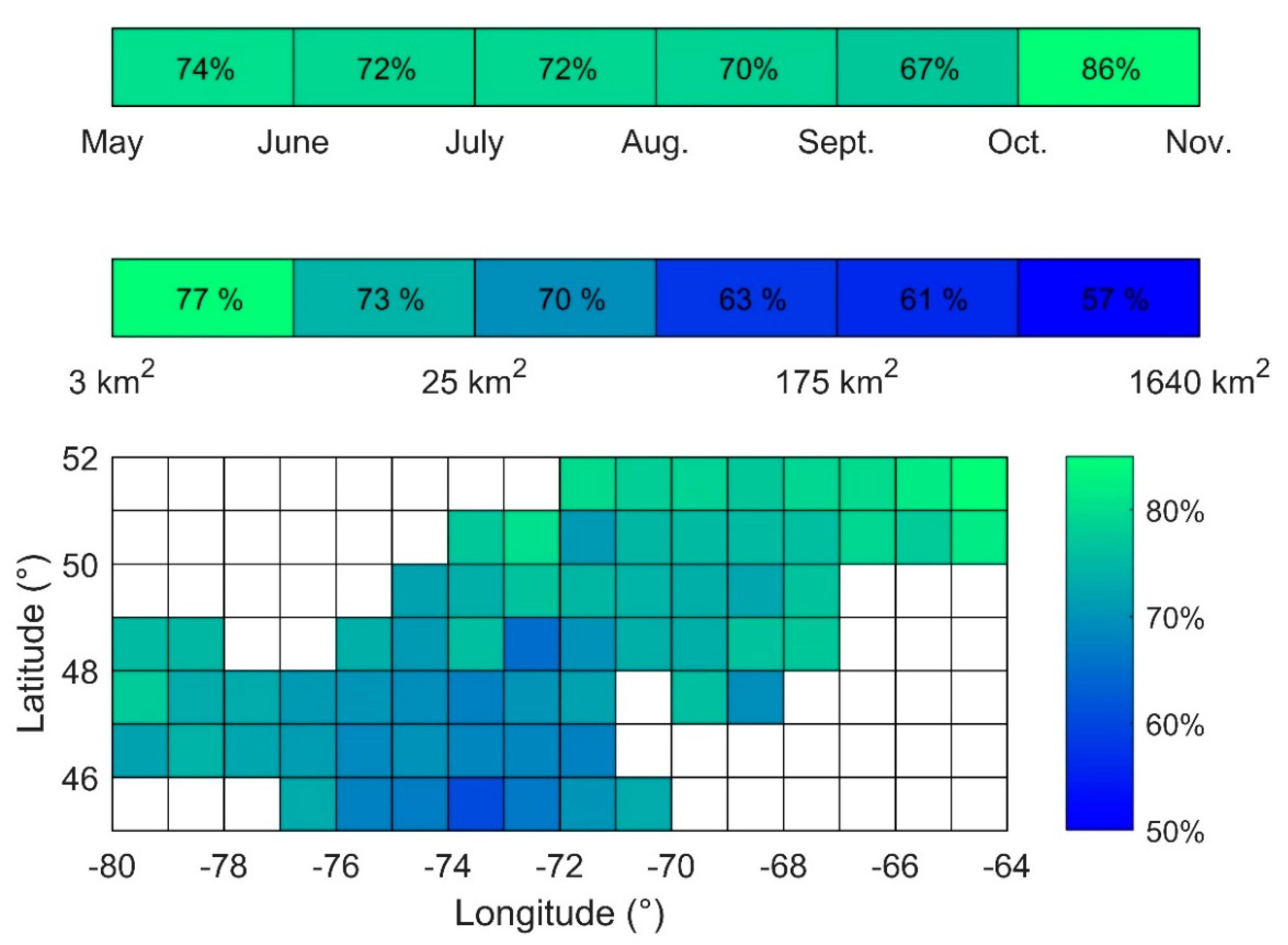
3.2. Frequency of Blooms

Bloom frequency shows a clear spatial pattern across the entire studied territory (Figure 4a,b). Phytoplankton blooms were more frequent west of the area, and this frequency tended to drop systematically from west to east (Kruskal-Wallis test (KW): χ 2 = 934; p < 0.001). A systematic increase was also apparent from north to south (KW: χ 2 = 433; p < 0.001). Hence, regions located in southwest Quebec had much more frequent blooms. In terms of temporal patterns, the median number of days with blooms increased by 23% between 2000 and 2016 (significant at the 10% threshold, p = 0.091; Figure 4). There was also a significant increase in high bloom frequencies; for example, the 95th percentile of the number of days with blooms increased by 24% between 2000 and 2016 (significant at the 5% threshold, p = 0.043; not presented). Conversely, smaller occurrence frequencies (5th percentile) did not show any significant trend over time. This generally concerns lakes located in underdeveloped regions, northeast of the studied area.

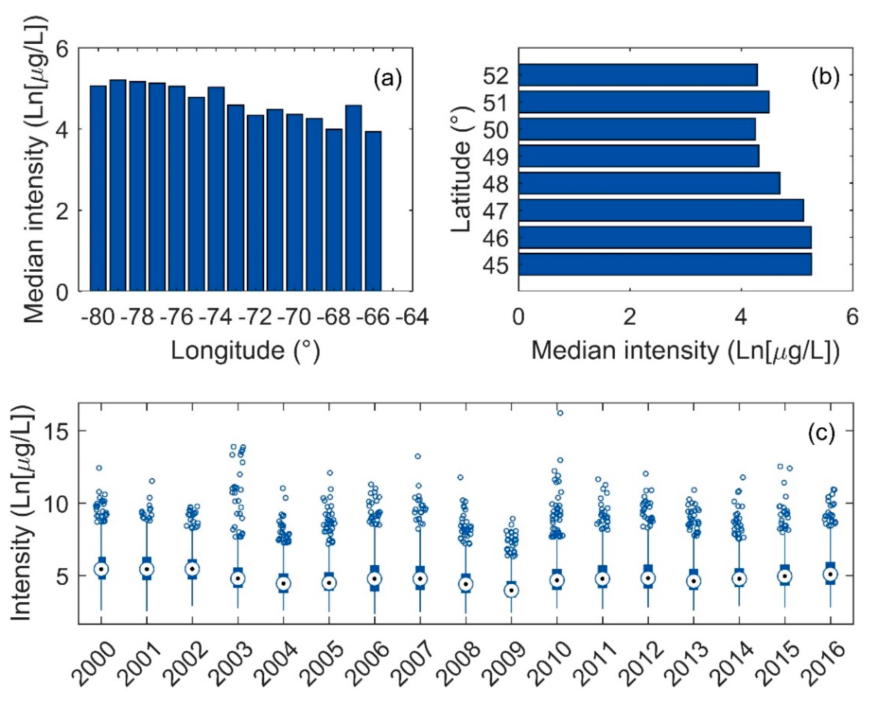
3.3. Intensity of Blooms

Although not marked as the frequency of occurrence, bloom intensity also showed a similar spatial pattern on the studied territory (Figure 5), representing an increase from east to west (KW: χ 2 = 199; p < 0.001) and from north to south (KW: χ 2 = 78; p < 0.001). No temporal trends of bloom intensity were detected between 2000 and 2016 (median, p = 0.220).

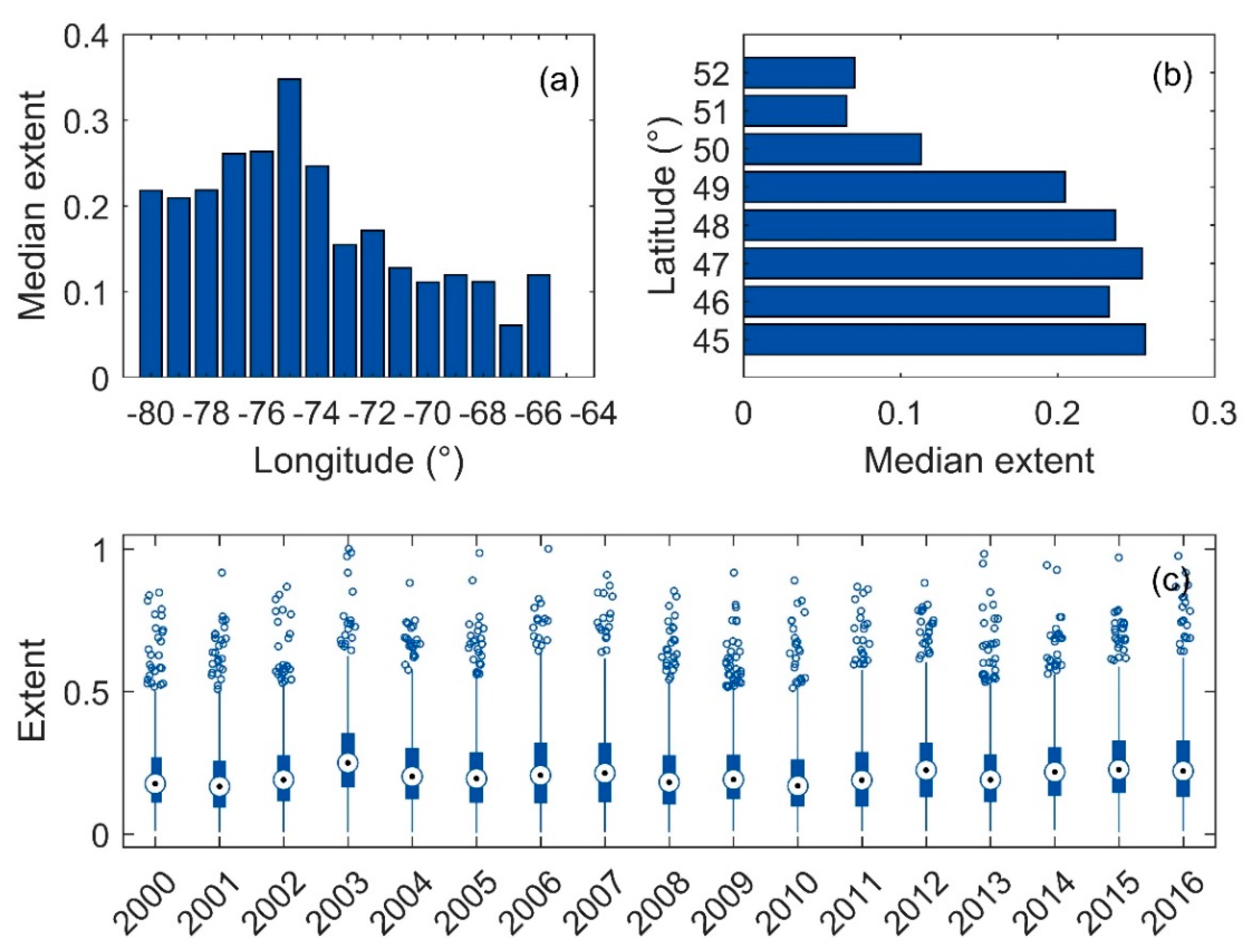
3.4. Surface Area of Blooms

The relative surface area of blooms showed a significant spatial pattern that differed from its frequency or intensity (Figure 6). The relative surface area significantly increased on lakes located between 74° W and 75° W (KW: χ 2 = 512; p < 0.01). It also increased from north to south, with blooms on lakes located between 45° N and 49° N showing a surface area twice as large as the lakes located between 50° N and 52° N (KW: χ 2 = 198; p < 0.01). This spatial trend was similar when the four fluvial lakes were removed from the dataset. No significant temporal trend in median surface area was observed between 2000 and 2016 (p = 0.1836). However, events characterized by large surface areas (95th percentile) significantly increased from 50 to 55% between 2000 and 2016 (p = 0.025).

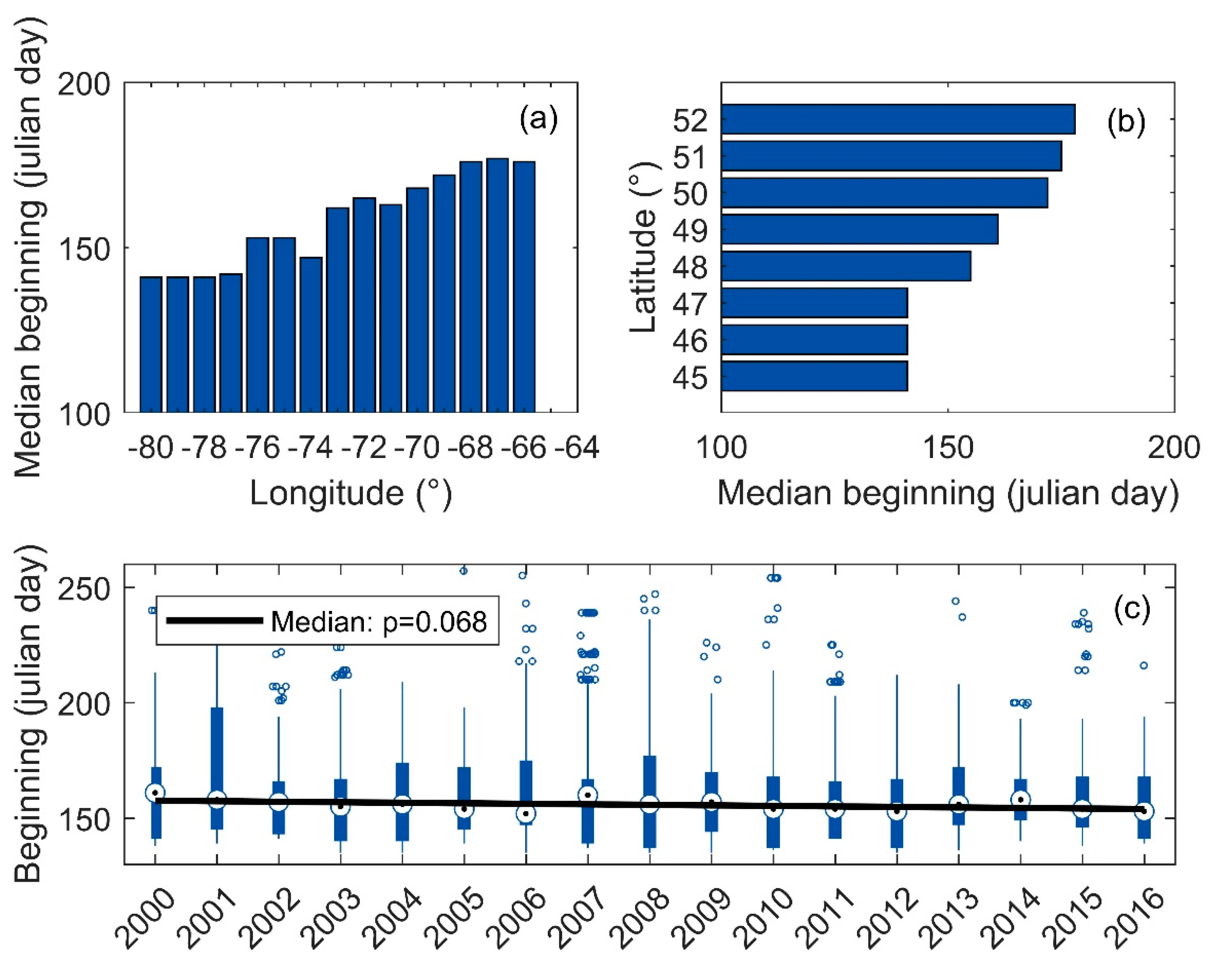
3.5. Onset Date of Blooms

The date of the first algal bloom was earlier on lakes located west of the studied area (Figure 7). The median date of the first event was May 21 at 80° W, while the first event occurred on 25 June at 66° W (KW: χ 2 = 828; p < 0.01). The first bloom also occurred increasingly early on lakes located further south of the territory (KW: χ 2 = 508; p < 0.01); for example, the median date of the first event was May 21 at 45° N, and 27 June at 52° N. For 58% of the lakes, the onset of blooms occurred before the beginning of July, while only 17 lakes had their bloom onset date later than 1 September (Figure 3d). Moreover, the first bloom occurred earlier as years progressed (p = 0.0646; Figure 7c); the median date for all lakes of the studied territory moved from 6 June to 3 June. The 95th percentile of the onset date (i.e., on the lakes with the latest onset date) also occurred earlier (yet not significant at a threshold of 10%, p = 0.1065), changing from July 14 to July 1 between 2000 and 2016. These lakes are typically located north of the studied area, with very little agricultural and urban development. Lakes characterized by the 5th percentile of the onset date, typically located southwest of the studied area in highly urbanized and agricultural sectors did not show any significant trend, the date remaining between 18 and 19 May from 2000 to 2016 (p = 0.826).

3.6. Phenological Trends of Missisquoi Bay and Lake Brome

The phenological trends of Missisquoi Bay (Lake Champlain; Figure 8) and Lake Brome (Figure 9) are presented since they have been extensively studied in the past given the persistence of cyanobacterial blooms on those lakes in the last decades. The annual occurrence frequency increased significantly on Missisquoi Bay, where the number of days above the Chl-a threshold increased from 25 in 2000 to 47 in 2016 (t = 2.71; p = 0.02). The intensity and surface area of these bloom events were important, with maximum Chl-a concentrations reaching 1315   μ g   L 1 on average every year, and surface area reaching 62 % . However, the onset date of blooms over Missisquoi Bay did not show any significant temporal trend. With regard to Lake Brome, the annual frequency also showed a significant increase from 23 days in 2000 to 30 days in 2016 (t = 2.32; p = 0.03). Although the intensity ( 219   μ g   L 1   on average) was lower than that of Missisquoi Bay, the bloom was covering the entire surface of the lake (maximum annual surface area reaching 100%) at least once every year over the studied period except in 2010 (97% of surface area). Although not significant, the first annual bloom occurred increasingly early in the spring on this lake (in average, from 28 May 2000 to 19 May 2016). This trend may be confirmed in the future.

3.7. Correlation Analysis

Results of the Pearson correlation analyses within and between the phenological and environmental variables are presented in Appendix B and Appendix C. These analyses allowed to reduce the number of environmental variables in order to eliminate information redundancy and to select variables most correlated to bloom phenology. Results indicate that the frequency of events and the onset date show a strong correlation with degree-days, while bloom intensity is correlated to water body morphology and water surface temperature. However, the bloom extent did not show any significant correlation with the environmental variables included in this study.

3.8. Canonical Correlation Analysis

Results from the CCA applied between the environmental variables and phytoplankton bloom phenology show high R i for the first two pairs of canonical variables (0.77 and 0.71), which considerably dropped for the last canonical correlations (0.23 and 0.13). The Bartlett test has shown that these canonical correlations are significant at threshold α = 0.01 (Table 2). Based on these R i values, only results of the first two pairs of canonical variables were interpreted. Table 3 presents the standardized canonical coefficients, structure coefficients, and communality coefficients. Communality coefficients where h 2 45 % are highlighted to identify the variables most useful to the canonical model development.

3.8.1. Phenological Variables

The phenological variable most contributing to the correlation between U1 was V1 were the frequency of occurrence (a1,1 = −0.54), followed by the onset date (a1,4 = 0.41), the intensity (a1,2 = −0.20), and the extent of blooms (a1,3 = −0.06). Variables with the highest level of relevance to the model development appear in the same order: the frequency of occurrence ( R ( V 1 , x 1 , 1 ) =     0.94 ), the onset date ( R ( V 1 , x 1 , 4 ) = 0.89 ), the intensity ( R ( V 1 , x 1 , 2 ) =     0.49 ), and the extent ( R ( V 1 , x 13 ) =     0.46 ). Hence, bloom phenology was mainly characterized by the frequency and onset date, followed by the intensity also having a significant contribution. These variables each provide complementary information, since they do not show strong collinearity ( r < 0.7 , Appendix B). The structure coefficients of frequency, intensity, and extent are inversely related to the structure coefficients of the onset date. Hence, high frequency, intensity, and large blooms are more likely to occur earlier in the open-water season. With regard to the second function, there was a significant contribution by the extent (a2,3 = 0.73; R ( V 2 , x 1 , 3 ) =   0.70 ), the intensity (a2,2 = −0.69; R ( V 2 , x 1 , 2 ) = 0.66 ), the onset date (a2,4 = −0.22; R ( V 2 , x 1 , 4 ) = 0.22 ), and finally the frequency (a2,1 = −0.21; R ( V 2 , x 1 , 1 ) = 0 ).

3.8.2. Environmental Variables

The environmental variables most contributing to the canonical correlation between U1 and V1 are the degree-days (b1,13 = −0.56; R ( U 1 , x 2 , 13 ) =     0.94 ), the percent cover by urban area (b1,7 = −0.37; R ( U 1 , x 2 , 7 ) =     0.65 ), the lake area (b1,1 = -0.36; R ( U 1 , x 2 , 1 ) = 0.38 ), the population ecumene (b1,9 = −0.22; R ( U 1 , x 2 , 9 ) = 0.48 ), the percent cover by forest (b1,6 = −0.20; R ( U 1 , x 2 , 6 ) = 0.38 ), and the lake watershed area (b1,3 = 0.21; R ( U 1 , x 2 , 3 ) = 0.19 ). Thus, degree-days and urban areas correspond to the climatic and physiographic characteristics most related to bloom phenology, and show a direct correlation with frequency, intensity, and extent of the blooms (r of same sign). The environmental variables mostly contributing to the second function of the canonical correlation are the lake area (b2,1 = −0.89; R ( U 2 , x 2 , 1 ) = 0.86 ) and precipitation (b2,11 = 0.26; R ( U 2 , x 2 , 11 ) = 0.44 ). All phenological variables contributed to the development of the first two pairs of canonical variables (h2 45%), while lake area, watershed area, land use (urban areas), and annual degree-days are the environmental variables that contributed the most.

4. Discussion

This study presents the spatiotemporal dynamics of phytoplankton blooms over 580 lakes in southern Quebec between 2000 and 2016, and their potential relationships with physiographic, morphological, and climatic descriptors prevailing on the lakes and their watersheds. The results demonstrate realistic and expected trends, which validate the usefulness of this approach to study the response of lake trophic state to historical and future changes in land use and climate. For instance, the data show the expected increase in the magnitude of phytoplankton blooms (expressed by frequency, surface area, or intensity) from north to south and east to west, as well as an earlier onset date in the southern and western regions of the studied region. These spatial trends had been observed over the last decades by water quality monitoring services (MELCC) [66,67,68], with blooms typically located in sectors of highly developed areas.
A particularly interesting result is the temporal increase of blooms observed between 2000 and 2016 in Quebec lakes, invalidating the hypothesis that the increasing trend would simply be related to the greater attention given to the phenomenon. This trend has also been observed by Winter et al. [69] from 1994 to 2009 on lakes of Ontario, and Ho et al. [42] over a 30-year period on 71 large lakes across the planet. The recent review by Huisman et al. [70] particularly describes the overall increase in frequency, intensity, and duration of cyanobacterial blooms observed on lakes globally. For example, this was demonstrated from the analysis of cyanobacterial pigments in sediment cores from over one hundred lakes of Northern America and Europe [71]. Our study allowed to quantify phenological trends over time and with respect to landscape characteristics, promoting predictive models such as the one put forward by Cremona et al. [17], who developed a cyanobacterial biomass prediction model with respect to regional climatic variables and hydrological indicators. They found that cyanobacteria biomass will increase from 2% to 10% in future decades.

4.1. Phenological Trends

During the period under study, phytoplankton biomass exceeded the threshold of 10 µg Chl-a L−1 during 15 days per year (May to October) on average for all lakes studied. This result is rather conservative, as only days with a cloud cover under 25% of observable surface area were included in the database, while we can assume that many additional cloudy days would add to this [27]. The areal extent of the blooms reached 19% of the overall lake surface on average (47% for the 95th percentile). Hence, most bloom events were rather restricted in terms of surface coverage. A bloom is qualified as very limited when the surface area remains under 25% (Sylvie Blais from the government of Quebec, pers. comm.). Our results show that all studied lakes had at least one pixel reaching a biomass of 10   μ g   Chl - a   L 1 or above at least once over the studied period, while this proportion drops to 12% of the lakes for blooms (biomass > 10 µg L−1) covering more than 50% of the lake area. Therefore, high biomass values are often reached, but the problem is seldom extended to the entire lake surface area.
High annual bloom frequencies were mostly observed on lakes located in highly developed sectors with heavy urbanization and agricultural use. The impact of land use (and its associated inputs of nutrients) appears to play an undeniable role on algal bloom phenology; this relationship was validated by the CCA showing that the relative proportion of urban areas and population ecumene were significant in controlling the frequency, intensity, and onset date. These results were also obtained by Weber et al. [72] showing a significant relationship between percent forest and cyanobacteria cell densities for 771 waterbodies in Georgia, USA. The bloom areal extent also varied spatially, with a significant increase between longitudes 74° W and 75° W, a corridor with intense seasonal resort operations stretching southwest of Montreal. However, this regional increase was partly caused by the phenology of two fluvial lakes (see Appendix D), Lake Des-Deux-Montagnes and Lake Saint-François, showing extended blooms (on average 35% of the lake area) of low biomass (median values below 15 µg L−1 for days exceeding the threshold). Nevertheless, this spatial trend in bloom areal extent still existed when removing fluvial lakes from the database.
An increase by 23% in bloom frequency was observed between 2000 and 2016 (all lakes). It was mostly observed on lakes with moderate to high frequencies (i.e., between 15 to 28 days of blooms per year on average). While the median areal extent did not increase significantly over the studied period, events covering a large fraction of the lake (95th percentile) showed a significant increase over the years. Hence, lakes with large and frequent blooms, for instance Missisquoi Bay north of Lake Champlain and Lake Brome, are the ones most clearly showing a rising trend over the studied period. These two lakes have largely been studied due to the intensity of blooms occurring there and the resulting socio-economic issues, for example on drinking water quality [10,73,74,75]. The rising importance of blooms on these lakes, often composed of buoyant cyanobacteria, has been associated to land-use changes (nutrient inputs) and increasing water temperature [76].
The first blooms occurred 3 days earlier in 2016 than in 2000 on average over the studied territory, although the accuracy of onset date estimates is influenced by the amount of missing data. Other studies have shown bloom onset date becoming earlier over time on Lake Taihu in China (subtropical climate), but at a much faster rate (~10 days earlier per year between 1998 and 2009, [38,77]). Interestingly, our results show that the onset date was particularly getting earlier (by almost 2 weeks) on lakes located in the northern part of the studied territory, but this specific trend is not significant. Direct impacts of increased air temperatures include an extended summer season, higher surface water temperatures, and intensified thermal stratification of lacustrine environments [78]. These conditions can stimulate the growth of phytoplankton communities in eutrophic environments [79] and particularly of cyanobacteria [70]. Therefore, these effects may be more apparent in northern regions where other anthropogenic factors are not acting, although the observed trends need to be substantiated.

4.2. Links to Climate and Environmental Physiography

It is not simple to identify the causes of the rising trend in bloom frequency in a context of population expansion occurring in parallel to global warming. Partitioning the causes will need the development of a regional model allowing to test various scenarios for a given water body with respect to the specific conditions prevailing on its watershed. The spatiotemporal trends in bloom onset date, development, maintenance, and decline observed on the studied territory present linkages with the lake’s morphological characteristics, watershed’s physiographic characteristics, and prevailing climatic conditions, as shown from the canonical analysis. It allowed to highlight the characteristics underpinning the regional dynamics of phytoplankton blooms.
The frequency and onset date of blooms are the phenological variables most strongly linked to the environmental characteristics prevailing on the lakes and their watershed. The most significant environmental variables are the lake area, watershed area, settlement, and degree-days. Ultimately, the input of nutrients to lakes will be larger in urbanized and agricultural sectors southwest of the territory where lakes are more exposed to non-point source pollution (typically related to agriculture) and point source pollution (e.g., sewage systems, domestic, or industrial wastes). On the other hand, since the studied territory covers about 600,000 km2, climate is very likely to play a role on phytoplankton bloom phenology. For example, on the studied territory, there is a difference of 37 days in the onset date of phytoplankton bloom. Zhang et al. [38] showed that the onset date and duration of blooms are strongly related to climate (temperature, sunshine hours, and global radiation). The southwestern part of the territory is therefore offering more favorable conditions to phytoplankton growth, particularly when nutrients are abundant (Huisman et al [70] and references therein).
Results indicate that the urbanized area is the physiographic variable best explaining bloom frequency and intensity. This relationship has been evoked in other studies mentioning that key forcing factors for the development of blooms include modifications resulting from anthropogenic activities such as contaminants from effluent and stormwater discharges, natural resource extraction and agricultural runoff [80,81]. Interestingly, the CCA results indicate that urbanization (settlement and population ecumene) better explains the spatiotemporal variability of phytoplankton blooms than agricultural variables (cropland and agriculture ecumene), but both variables are linked on this relative occupancy scale. In the studied region, urban area varied extensively (0–64% of the lakes drainage basin) as well as farming area (0–55%). Farming has often been raised as a major controlling factor on bloom phenology through its influence on P and N loads.
The impact of lake surface area on frequency, intensity, and onset date revealed in the present study (larger lakes presenting higher frequency, intensity, and earlier onset date) has yet to be explained, although lake morphology is of definite importance in the development of cyanobacteria. For instance, dominance of filamentous species is observed in shallow lakes while colony-forming species dominate deeper lakes [82]. Others have also shown the influence of hydrologic retention time on the establishment of blooms and their composition [83,84]. Since larger lakes generally tend to have longer retention times, this factor could explain the relationships revealed by the CCA. However, we cannot exclude that the frequency of events could increase with the observable lake surface area (by the remote sensor), increasing the probability of detecting a bloom.
Degree-days is the climatic variable best explaining bloom phenology, followed by total annual precipitation. However, annual or seasonal water temperatures (Table 3 and Appendix C) do not show any clear relationships with the phenological variables. Although several temperature descriptors have often been related to phytoplankton growth, including atmospheric temperature [19,38], water temperature [85], hours of sunlight [38], and degree-days [86,87], it is the latter descriptor that most directly impact the growth of ectotherm organisms [88]. For instance, Ralston et al. [87] used degree-days to assess inter-annual variability in the onset date of algal blooms, their development and date of decline in the Nauset estuary, and proposed this metric as an efficient warning indicator. Trombetta et al. [89] also pointed out that water temperature is a key factor controlling the phenology and community structure of phytoplankton blooms in a Mediterranean shallow coastal system. The recent study by Ho and Michalak [90], exploiting over twelve hundred summertime lake observations from across the continental U.S., showed that summer temperature drives total phytoplankton abundance, while the length of summer is linked to cyanobacterial abundance. The impact of precipitations on bloom frequency, intensity, and onset date suggested by the present study CCA is also discussed by Ho and Michalak [90], who are evoking the effect of increased nutrient runoff on bloom development, while precipitations could rise flushing rates and slow down growth, confusing the relationships.

5. Conclusions

This study provides a regional portrait of lake trophic state over a wide variety of lacustrine environments in Quebec, and a detailed phenology allowing to go beyond simple biomass assessments at the scale of a lake or locally. It offers an approach to characterize bloom phenology on lakes that are providing ecological services for instance, and eventually to forecast how this phenomenon could evolve in response to changes in climate or land use. This approach is of particular interest in a country with over a million lakes across its territory [91]. While the statistical approach used here does not provide definitive mechanistic linkages, it is useful for identifying potential mechanisms driving bloom phenology at the regional scale. The increasing frequency of bloom events observed over the study period invalidates the hypothesis that the rising trend would simply be due to the greater amount of attention given to the phenomenon. Remote sensing data allows to assess bloom phenology with much more details and inform on specific features. For example, results indicate that high biomass values are often reached but the problem is seldom extended to the entire lake surface. Moreover, studying blooms over a territory 600,000 km2 allowed to determine a difference in bloom onset dates of 37 days, which could be exploited in a space-for-time substitution approach to assess the response of lakes to future climate conditions.
The analysis of bloom phenology on 580 lakes and the associated environmental conditions also allowed to identify key factors explaining the spatiotemporal patterns: degree-days, land use, and the morphology of lakes and their watersheds. For instance, the procedure adopted here based on remote sensing provides near-real time biomass estimation to implement management plans in a recreational context. Remote sensing offers a great potential to locate where phytoplankton blooms initiate and how they evolve over space and time, and exploit regional relationships to study local patterns. This will be done through the development of a statistical model examining the impact of climate or land use on the occurrence of phytoplankton blooms, which will be presented in a sister paper. As spatial resolution improves and images become more accessible, this approach will represent an efficient tool to identify priority areas and strategies in restoration plans.

Author Contributions

Formal analysis, C.R.-F.; Funding acquisition, C.R.-F.; Methodology, C.R.-F.; Supervision, K.C. and I.L.; Validation, C.R.-F.; Writing—original draft, C.R.-F.; Writing—review & editing, K.C. and I.L. All authors have read and agreed to the published version of the manuscript.

Funding

This work was funded by the Fonds Québécois de la Recherche sur la Nature et les Technologies (FQRNT), the Institut national de la recherche scientifique (INRS), and the Interuniversity Research Group in Limnology (GRIL).

Acknowledgments

We are grateful to Sylvie Blais and Nathalie Bourbonnais from the Ministère de l’Environnement et de la Lutte contre les Changements Climatiques for their precious assistance when comparing remote sensing trends to in situ observations, and the Interuniversity Research Group in Limnology who provided in situ observations. Two anonymous reviewers provided valuable comments on the manuscript. NARR data were obtained from the NOAA/OAR/ESRL PSD, Boulder, CO, USA, through their website at https://www.esrl.noaa.gov/psd/.

Conflicts of Interest

The authors declare no conflict of interest.

Appendix A. Uncertainties on the Estimation of Pytoplankton Biomass and Global Trends

Naturally, there is an uncertainty regarding the Chl-a concentration values obtained using the ensemble-based model developed by El Alem et al. [48]. This model had a determination coefficient of 0.93 (relative RMSE = 50%, relative BIAS = −27%, relative NASH = 0.70) when it was tested on an independent database containing a group of lakes with relatively low biomass in the southern part of the studied territory, and where Chl-a concentrations had been measured in-situ [48]. Using a cross-validation approach, the model performed better when it was used to estimate high Chl-a concentrations (R2 = 0.98, RMSEr = 15%, BIASr = −2%, NASHr = 0.95) than at the initialization of blooms (R2 = 0.77, RMSEr = 37%, BIASr = −8%, and NASHr = 0.70). The model calibration did not include fluvial environments, where the hydrological dynamics and optically active components are different from those of lacustrine environments, and where there is a greater amount of suspended inorganic matter. This could cause an estimation bias regarding Chl-a concentrations when non-algae particles are proportionally concentrated, although a qualitative evaluation of this type of interference by El Alem et al. [48] seems to indicate that the estimation model behaved correctly in the presence of a high inorganic content in Lake Huron. That is why the results of lakes Des-Deux-Montagnes, Saint-Louis, Saint-François, and Saint-Pierre, located along the St. Lawrence River, were presented for information purposes only. The inclusion of these lakes does not affect our global results, since the spatiotemporal trend analysis and the CCA were also carried out without including these lakes, and the results remained the same. In Lake Des-Deux-Montagnes, bordering the city of Montréal, the median summer concentration of Chl-a was 4.8 µg L−1 in 2000 according to our results, while in situ measurements taken close to the lake in 1997–1998 varied between 2 and 5 µg L−1 [66]. Given the little amount of data available to validate the estimations obtained for these lakes, it is difficult to ensure of the accuracy of the concentrations, further justifying the need to develop this type of approach when aiming to describe the phenological history of phytoplankton blooms using remote sensing.
Lastly, the percentage of missing data due to a large cloud cover (over 75% of the lake’s surface area) or to geometric distortion of MODIS images was 68% at 45° N for the present study, which gradually increased with latitude, reaching 80% of missing data at 52° N (Figure A1). The number of sunlight hours in Quebec [92,93] fully explains the spatial variability of missing data. Certain studies have shown that missing data can affect the accuracy of phenological variables, particularly on phytoplankton bloom frequency and onset date. For example, Cole et al. [94] found bloom onset date errors in ocean environments of the order of 2 to 3 days with 10% of missing data, and 15 to 30 days with 80% missing data when using images from the SeaWiFS sensor. The results obtained in the present study obviously carry an uncertainty related to cloud cover, which is admittedly difficult to quantify. Nonetheless, satellite databases considerably increase the precision and accuracy of spatiotemporal modelling of phytoplankton blooms comparatively to in situ sampling, thus representing a fair trade-off.
Figure A1. Mean percentage (%) of missing data (between 2000 and 2016) related to cloud cover covering more than 75% of the lake for a given lake, or having geometric distortion of the MODIS image. The mean percentage of days with missing data is shown on the bases of months, lake surface area and location (latitude and longitude).
Environments 07 00077 g0a1

Appendix B

Table A1. Pearson correlation analysis between bloom phenological and environmental variables.
FrequencyIntensitySurface AreaOnset
Lake morphologyArea0.090.21−0.01−0.02
Perimeter0.160.54−0.10−0.05
Gravelius coefficient0.220.50−0.18−0.11
Length of the Gravelius’s rectangle0.160.54−0.10−0.05
Width of the Gravelius’s rectangle0.150.25−0.01−0.03
Watershed morphologyArea0.160.270.06−0.05
Perimeter 0.180.37−0.03−0.06
Gravelius coefficient0.210.34−0.12-0.12
Length of the Gravelius’s rectangle0.180.37−0.03−0.06
Width of the Gravelius’s rectangle0.210.46−0.04−0.05
Slope—mean0.100.040.09−0.04
Slope—standard deviation−0.24−0.09−0.140.22
PhysiographyLand cover—Forest0.160.280.04−0.05
Land cover—Settlement0.170.130.16−0.07
Land cover—Cropland0.200.160.21−0.08
Land cover—Forest (relative)−0.33−0.10−0.210.17
Land cover—Settlement (relative)0.290.070.16−0.22
Land cover—Cropland (relative)0.300.100.20−0.13
Population ecumene0.320.060.25−0.30
Agriculture ecumene0.280.090.19−0.14
ClimateTotal precipitation—annual−0.23−0.430.020.11
Total precipitation—summer−0.22−0.350.010.09
Mean temperature—annual−0.13−0.470.030.00
Mean temperature—summer−0.13−0.470.030.01
Wind speed—annual0.020.020.08−0.04
Wind speed—summer0.090.060.08−0.08
Degree-days above 20 °C0.610.160.35−0.55

Appendix C

Table A2. Pearson correlation analysis among environmental variables (left) and among bloom phenological variables (right). L = lake; W = watershed; rel = relative %.
FrequencyIntensityExtentOnset Date
L Area1 10.320.29−0.66Frequency
L Perimeter0.501 10.03−0.16Intensity
L Shape index0.130.791 1−0.32Extent
L Length 0.481.000.801 1Onset date
L Width0.900.390.000.371
W Area0.570.520.290.510.601
W Perimeter 0.570.620.440.610.590.891
W Shape index0.260.430.500.430.240.410.691
W Length 0.570.610.440.600.590.891.000.691
W Width0.470.720.540.710.520.850.870.500.861
Slope—mean0.010.110.130.110.010.590.370.100.370.431
Slope—std0.05−0.04−0.04−0.040.01−0.08−0.030.08−0.03−0.08−0.111
Forest0.550.520.300.510.591.000.900.420.900.860.57−0.081
Settlement0.220.240.160.240.230.810.600.200.590.650.88−0.140.781
Cropland0.210.240.150.240.250.770.590.200.590.660.72−0.150.750.951
Forest (rel)−0.06−0.060.01−0.06−0.17−0.13−0.13−0.04−0.13−0.24−0.090.20−0.11−0.21−0.301
Settlement (rel)0.030.02−0.040.020.110.080.060.010.060.110.08−0.100.070.150.18−0.761
Cropland (rel)0.060.070.010.070.170.130.140.050.140.260.07−0.220.110.210.31−0.960.551
Population ecumene0.040.01−0.040.000.110.070.060.000.060.120.05−0.040.060.110.14−0.540.620.431
Agriculture ecumene0.080.070.010.070.170.130.140.050.140.240.06−0.200.110.190.27−0.870.630.850.481
Total pcp—annual−0.29−0.54−0.40−0.54−0.30−0.41−0.42−0.22−0.42−0.54−0.140.04−0.41−0.27−0.300.21−0.18−0.20−0.13−0.181
Total pcp—summer−0.22−0.41−0.30−0.40−0.22−0.31−0.31−0.16−0.31−0.40−0.11−0.03−0.30−0.20−0.230.16−0.14−0.15−0.12−0.140.881
Mean temp—annual−0.43−0.79−0.56−0.79−0.44−0.60−0.62−0.30−0.62−0.79−0.210.05−0.60−0.39−0.430.13−0.04−0.15−0.01−0.120.670.501
Mean temp—summer−0.43−0.79−0.56−0.79−0.44−0.60−0.62−0.30−0.62−0.79−0.210.05−0.60−0.39−0.430.14−0.04−0.16−0.02−0.120.670.511.001
Wind—annual−0.01−0.01−0.02−0.010.00−0.03−0.04−0.07−0.04−0.02−0.01−0.12−0.02−0.02−0.02−0.110.130.080.040.040.000.040.010.021
Wind—summer−0.06−0.010.01−0.01−0.04−0.06−0.08−0.08−0.08−0.04−0.02−0.25−0.06−0.04−0.04−0.040.040.03−0.05−0.010.040.060.020.020.731
Degree days−0.090.000.060.00−0.060.010.010.080.010.020.07−0.260.010.080.09−0.240.260.200.270.21−0.13−0.130.020.020.100.181
L AreaL PerimeterL Shape indexL Length L WidthW AreaW Perimeter W Shape indexW Length W WidthSlope—meanSlope—stdForestSettlementCroplandForest (rel)Settlement (rel)Cropland (rel)Pop ecumeneAgr ecumenePcp—annualPcp—summerTemp—annualTemp—summerWind—annualWind—summerDegree days

Appendix D

Figure A2. Localization of Lake Des-Deux-Montagnes, Lake Saint-Louis, Lake Saint-François, Lake Brome, and Missisquoi Bay of Lake Champlain.
Environments 07 00077 g0a2

References

  1. Michalak, A.M.; Anderson, E.J.; Beletsky, D.; Boland, S.; Bosch, N.S.; Bridgeman, T.B.; Chaffin, J.D.; Cho, K.; Confesor, R.; Daloglu, I. Record-setting algal bloom in Lake Erie caused by agricultural and meteorological trends consistent with expected future conditions. Proc. Natl. Acad. Sci. USA 2013, 110, 6448–6452. [Google Scholar] [CrossRef] [PubMed] [Green Version]
  2. Higgins, S.N.; Pennuto, C.M.; Howell, E.T.; Lewis, T.W.; Makarewicz, J.C. Urban influences on Cladophora blooms in Lake Ontario. J. Great Lakes Res. 2012, 38, 116–123. [Google Scholar] [CrossRef]
  3. Duan, H.; Loiselle, S.A.; Zhu, L.; Feng, L.; Zhang, Y.; Ma, R. Distribution and incidence of algal blooms in Lake Taihu. Aquat. Sci. 2015, 77, 9–16. [Google Scholar] [CrossRef]
  4. Rosen, B.H.; Davis, T.W.; Gobler, C.J.; Kramer, B.J.; Loftin, K.A. Cyanobacteria of the 2016 Lake Okeechobee and Okeechobee Waterway Harmful Algal Bloom; No. 2017-1054; US Geological Survey: Reston, VA, USA, 2017. [CrossRef] [Green Version]
  5. Simiyu, B.M.; Oduor, S.O.; Rohrlack, T.; Sitoki, L.; Kurmayer, R. Microcystin Content in Phytoplankton and in Small Fish from Eutrophic Nyanza Gulf, Lake Victoria, Kenya. Toxins 2018, 10, 275. [Google Scholar] [CrossRef] [PubMed] [Green Version]
  6. Chorus, I.; Bartram, J. Toxic Cyanobacteria in Water: A Guide to Their Public Health Consequences, Monitoring and Management; CRC Press: Boca Raton, FL, USA, 1999. [Google Scholar]
  7. Steffensen, D.A. Economic cost of cyanobacterial blooms. In Cyanobacterial Harmful Algal Blooms: State of the Science and Research Needs; Springer: New York, NY, USA, 2008; Volume 619. [Google Scholar] [CrossRef]
  8. Zamyadi, A.; McQuaid, N.; Prévost, M.; Dorner, S. Monitoring of potentially toxic cyanobacteria using an online multi-probe in drinking water sources. J. Environ. Monit. 2012, 14, 579–588. [Google Scholar] [CrossRef] [PubMed]
  9. Hozumi, A.; Ostrovsky, I.; Sukenik, A.; Gildor, H. Turbulence regulation of Microcystis surface scum formation and dispersion during a cyanobacteria bloom event. Inland Waters 2020, 10, 51–70. [Google Scholar] [CrossRef]
  10. Wheeler, S.M.; Morrissey, L.A.; Levine, S.N.; Livingston, G.P.; Vincent, W.F. Mapping cyanobacterial blooms in Lake Champlain’s Missisquoi Bay using QuickBird and MERIS satellite data. J. Great Lakes Res. 2012, 38, 68–75. [Google Scholar] [CrossRef]
  11. Bonnet, M.; Poulin, M. DyLEM-1D: A 1D physical and biochemical model for planktonic succession, nutrients and dissolved oxygen cycling: Application to a hyper-eutrophic reservoir. Ecol. Model. 2004, 180, 317–344. [Google Scholar] [CrossRef]
  12. Janssen, F.; Neumann, T.; Schmidt, M. Inter-annual variability in cyanobacteria blooms in the Baltic Sea controlled by wintertime hydrographic conditions. Mar. Ecol. Prog. Ser. 2004, 275, 59–68. [Google Scholar] [CrossRef]
  13. Laanemets, J.; Lilover, M.-J.; Raudsepp, U.; Autio, R.; Vahtera, E.; Lips, I.; Lips, U. A fuzzy logic model to describe the cyanobacteria Nodularia spumigena blooms in the Gulf of Finland, Baltic Sea. Hydrobiologia 2006, 554, 31–45. [Google Scholar] [CrossRef]
  14. Onderka, M. Correlations between several environmental factors affecting the bloom events of cyanobacteria in Liptovska Mara reservoir (Slovakia)—A simple regression model. Ecol. Model. 2007, 209, 412–416. [Google Scholar] [CrossRef]
  15. Garnier, J.; Nemery, J.; Billen, G.; Théry, S. Nutrient dynamics and control of eutrophication in the Marne River system: Modelling the role of exchangeable phosphorus. J. Hydrol. 2005, 304, 397–412. [Google Scholar] [CrossRef]
  16. Couture, R.-M.; Tominaga, K.; Starrfelt, J.; Moe, S.J.; Kaste, Ø.; Wright, R.F. Modelling phosphorus loading and algal blooms in a Nordic agricultural catchment-lake system under changing land-use and climate. Environ. Sci. Process. Impacts 2014, 16, 1588–1599. [Google Scholar] [CrossRef] [PubMed] [Green Version]
  17. Cremona, F.; Vilbaste, S.; Couture, R.-M.; Nõges, P.; Nõges, T. Is the future of large shallow lakes blue-green? Comparing the response of a catchment-lake model chain to climate predictions. Clim. Chang. 2017, 141, 347–361. [Google Scholar] [CrossRef]
  18. Couture, R.-M.; Moe, S.J.; Lin, Y.; Kaste, Ø.; Haande, S.; Solheim, A.L. Simulating water quality and ecological status of Lake Vansjø, Norway, under land-use and climate change by linking process-oriented models with a Bayesian network. Sci. Total Environ. 2018, 621, 713–724. [Google Scholar] [CrossRef]
  19. Hu, W.; Connell, D.; Mengersen, K.; Tong, S. Weather variability, sunspots, and the blooms of cyanobacteria. EcoHealth 2009, 6, 71–78. [Google Scholar] [CrossRef]
  20. Liu, Y.; Wang, Z.; Guo, H.; Yu, S.; Sheng, H. Modelling the effect of weather conditions on cyanobacterial bloom outbreaks in Lake Dianchi: A rough decision-adjusted logistic regression model. Environ. Model. Assess. 2013, 18, 199–207. [Google Scholar] [CrossRef]
  21. Paerl, H.W. Controlling eutrophication along the freshwater–marine continuum: Dual nutrient (N and P) reductions are essential. Estuaries Coasts 2009, 32, 593–601. [Google Scholar] [CrossRef] [Green Version]
  22. Wang, Y.; Ma, H.; Sheng, D.; Wang, D. Assessing the interactions between chlorophyll a and environmental variables using copula method. J. Hydrol. Eng. 2011, 17, 495–506. [Google Scholar] [CrossRef]
  23. Davis, T.W.; Berry, D.L.; Boyer, G.L.; Gobler, C.J. The effects of temperature and nutrients on the growth and dynamics of toxic and non-toxic strains of Microcystis during cyanobacteria blooms. Harmful Algae 2009, 8, 715–725. [Google Scholar] [CrossRef]
  24. Guildford, S.J.; Hecky, R.E.; Smith, R.E.; Taylor, W.D.; Charlton, M.N.; Barlow-Busch, L.; North, R.L. Phytoplankton nutrient status in Lake Erie in 1997. J. Great Lakes Res. 2005, 31, 72–88. [Google Scholar] [CrossRef]
  25. Steffen, M.M.; Belisle, B.S.; Watson, S.B.; Boyer, G.L.; Wilhelm, S.W. Status, causes and controls of cyanobacterial blooms in Lake Erie. J. Great Lakes Res. 2014, 40, 215–225. [Google Scholar] [CrossRef]
  26. Chaffin, J.D.; Bridgeman, T.B.; Bade, D.L. Nitrogen constrains the growth of late summer cyanobacterial blooms in Lake Erie. Adv. Microbiol. 2013, 3, 16. [Google Scholar] [CrossRef] [Green Version]
  27. Duan, H.; Ma, R.; Zhang, Y.; Loiselle, S.A. Are algal blooms occurring later in Lake Taihu? Climate local effects outcompete mitigation prevention. J. Plankton Res. 2014, 36, 866–871. [Google Scholar] [CrossRef] [Green Version]
  28. Havens, K.E.; James, R.T.; East, T.L.; Smith, V.H. N: P ratios, light limitation, and cyanobacterial dominance in a subtropical lake impacted by non-point source nutrient pollution. Environ. Pollut. 2003, 122, 379–390. [Google Scholar] [CrossRef]
  29. Lilover, M.-J.; Stips, A. The variability of parameters controlling the cyanobacteria bloom biomass in the Baltic Sea. J. Mar. Syst. 2008, 74, 108–115. [Google Scholar] [CrossRef]
  30. Bergström, A.-K. The use of TN:TP and DIN:TP ratios as indicators for phytoplankton nutrient limitation in oligotrophic lakes affected by N deposition. Aquat. Sci. 2010, 72, 277–281. [Google Scholar] [CrossRef]
  31. Ptacnik, R.; Andersen, T.; Tamminen, T. Performance of the Redfield ratio and a family of nutrient limitation indicators as thresholds for phytoplankton N vs. P limitation. Ecosystems 2010, 13, 1201–1214. [Google Scholar] [CrossRef]
  32. Winder, M.; Berger, S.A.; Lewandowska, A.; Aberle, N.; Lengfellner, K.; Sommer, U.; Diehl, S. Spring phenological responses of marine and freshwater plankton to changing temperature and light conditions. Mar. Biol. 2012, 159, 2491–2501. [Google Scholar] [CrossRef]
  33. Mehnert, G.; Leunert, F.; Cirés, S.; Jöhnk, K.D.; Rücker, J.; Nixdorf, B.; Wiedner, C. Competitiveness of invasive and native cyanobacteria from temperate freshwaters under various light and temperature conditions. J. Plankton Res. 2010, 32, 1009–1021. [Google Scholar] [CrossRef]
  34. Paerl, H.W.; Hall, N.S.; Calandrino, E.S. Controlling harmful cyanobacterial blooms in a world experiencing anthropogenic and climatic-induced change. Sci. Total Environ. 2011, 409, 1739–1745. [Google Scholar] [CrossRef] [PubMed]
  35. Huisman, J.; Hulot, F.D. Population dynamics of harmful cyanobacteria. In Harmful Cyanobacteria; Springer: Berlin/Heidelberg, Germany, 2005; pp. 143–176. [Google Scholar] [CrossRef]
  36. Janssen, A.B.; Janse, J.H.; Beusen, A.H.; Chang, M.; Harrison, J.A.; Huttunen, I.; Kong, X.; Rost, J.; Teurlincx, S.; Troost, T.A. How to model algal blooms in any lake on earth. Curr. Opin. Environ. Sustain. 2019, 36, 1–10. [Google Scholar] [CrossRef]
  37. Reichwaldt, E.S.; Ghadouani, A. Effects of rainfall patterns on toxic cyanobacterial blooms in a changing climate: Between simplistic scenarios and complex dynamics. Water Res. 2012, 46, 1372–1393. [Google Scholar] [CrossRef] [PubMed]
  38. Zhang, M.; Duan, H.; Shi, X.; Yu, Y.; Kong, F. Contributions of meteorology to the phenology of cyanobacterial blooms: Implications for future climate change. Water Res. 2012, 46, 442–452. [Google Scholar] [CrossRef]
  39. Moss, B. Cogs in the endless machine: Lakes, climate change and nutrient cycles: A review. Sci. Total Environ. 2012, 434, 130–142. [Google Scholar] [CrossRef] [PubMed]
  40. Wagner, C.; Adrian, R. Cyanobacteria dominance: Quantifying the effects of climate change. Limnol. Oceanogr. 2009, 54, 2460–2468. [Google Scholar] [CrossRef]
  41. Bartosiewicz, M.; Przytulska, A.; Deshpande, B.N.; Antoniades, D.; Cortes, A.; MacIntyre, S.; Lehmann, M.F.; Laurion, I. Effects of climate change and episodic heat events on cyanobacteria in a eutrophic polymictic lake. Sci. Total Environ. 2019, 693, 133414. [Google Scholar] [CrossRef]
  42. Ho, J.C.; Michalak, A.M.; Pahlevan, N. Widespread global increase in intense lake phytoplankton blooms since the 1980s. Nature 2019, 574, 667–670. [Google Scholar] [CrossRef]
  43. Chapra, S.C.; Boehlert, B.; Fant, C.; Bierman Jr, V.J.; Henderson, J.; Mills, D.; Mas, D.M.; Rennels, L.; Jantarasami, L.; Martinich, J. Climate change impacts on harmful algal blooms in US freshwaters: A screening-level assessment. Environ. Sci. Technol. 2017, 51, 8933–8943. [Google Scholar] [CrossRef]
  44. Edwards, M.; Richardson, A.J. Impact of climate change on marine pelagic phenology and trophic mismatch. Nature 2004, 430, 881. [Google Scholar] [CrossRef]
  45. Winder, M.; Sommer, U. Phytoplankton response to a changing climate. Hydrobiologia 2012, 698, 5–16. [Google Scholar] [CrossRef]
  46. Venables, W.N.; Ripley, B.D. Modern Applied Statistics with S-PLUS; Springer Science & Business Media: Berlin, Germany, 2013; p. 487. [Google Scholar]
  47. Trishchenko, A.; Luo, Y.; Khlopenkov, K. A method for downscaling MODIS land channels to 250 m spatial resolution using adaptive regression and normalization. In Remote Sensing for Environmental Monitoring; International Society for Optics and Photonics: Bellingham, WA, USA, 2006; Volume 6366, p. 36607. [Google Scholar] [CrossRef]
  48. El-Alem, A.; Chokmani, K.; Laurion, I.; El-Adlouni, S.E.; Raymond, S.; Ratte-Fortin, C. Ensemble-Based Systems to Monitor Algal Bloom With Remote Sensing. IEEE Trans. Geosci. Remote. Sens. 2019, 57, 7955–7971. [Google Scholar] [CrossRef]
  49. Ratte-Fortin, C.; Chokmani, K.; El Alem, A. A novel algorithm for cloud detection over inland water bodies using 250m downscaled MODIS imagery. Int. J. Remote Sens. 2018, 39, 6429–6439. [Google Scholar] [CrossRef]
  50. World Health Organization. Guidelines for Safe Recreational Water Environments: Coastal and Fresh Waters; World Health Organization: Geneva, Switzerland, 2003; Volume 1, p. 253. [Google Scholar]
  51. Ministère du Développement durable, de l’Environnement, de la Faune & des Parcs. L’Eau. La Vie. L’Avenir. Politique Nationale De L’Eau; Bibliothèque nationale du Québec: Montréal, QC, Canada, 2002. [Google Scholar]
  52. Natural Resources Canada. Canadian Digital Elevation Model [Computer File]; Natural Resources Canada: Ottawa, ON, Canada, 2015. Available online: http://ouvert.canada.ca/data/fr/dataset/7f245e4d-76c2-4caa-951a-45d1d2051333 (accessed on 26 May 2017).
  53. Mesinger, F.; DiMego, G.; Kalnay, E.; Mitchell, K.; Shafran, P.C.; Ebisuzaki, W.; Jović, D.; Woollen, J.; Rogers, E.; Berbery, E.H. North American regional reanalysis. Bull. Am. Meteorol. Soc. 2006, 87, 343–360. [Google Scholar] [CrossRef] [Green Version]
  54. Dupuis, A.P.; Hann, B.J. Warm spring and summer water temperatures in small eutrophic lakes of the Canadian prairies: Potential implications for phytoplankton and zooplankton. J. Plankton Res. 2009, 31, 489–502. [Google Scholar] [CrossRef] [Green Version]
  55. Neuheimer, A.B.; Taggart, C.T. The growing degree-day and fish size-at-age: The overlooked metric. Can. J. Fish. Aquat. Sci. 2007, 64, 375–385. [Google Scholar] [CrossRef]
  56. Natural Resources Canada. Land Use 1990, 2000 & 2010. [Computer File]; Natural Resources Canada: Ottawa, ON, Canada, 2015. Available online: https://open.canada.ca/data/en/dataset/18e3ef1a-497c-40c6-8326-aac1a34a0dec (accessed on 17 August 2017).
  57. Natural Resources Canada. Population Ecumene Census Division. [Computer File]; Natural Resources Canada: Ottawa, ON, Canada, 2016. Available online: https://open.canada.ca/data/en/dataset/8498f9b4-4914-456c-9223-4260ea3bea4d (accessed on 17 August 2017).
  58. Kruskal, W.H.; Wallis, W.A. Use of ranks in one-criterion variance analysis. J. Am. Stat. Assoc. 1952, 47, 583–621. [Google Scholar] [CrossRef]
  59. Bradley, J.V. Distribution-Free Statistical Tests; Prentice-Hall: Upper Saddle River, NJ, USA, 1968; p. 388. [Google Scholar]
  60. Jarque, C.M.; Bera, A.K. Efficient tests for normality, homoscedasticity and serial independence of regression residuals. Econ. Lett. 1980, 6, 255–259. [Google Scholar] [CrossRef]
  61. Bartlett, M.S. A note on tests of significance in multivariate analysis. Math. Proc. Camb. Philos. Soc. 1939, 35, 180–185. [Google Scholar] [CrossRef]
  62. Johnson, R.; Wichern, D. Applied Multivariate Statistical Analysis, 6th ed.; Pearson Prentice Hall: London, UK, 2007; p. 265. [Google Scholar]
  63. Thompson, B. A primer on the logic and use of canonical correlation analysis. Meas. Eval. Couns. Dev. 1991, 24, 80–93. [Google Scholar]
  64. Zientek, L.; Thompson, B. Commonality analysis: Partitioning variance to facilitate better understanding of data. J. Early Interv. 2006, 28, 299–307. [Google Scholar] [CrossRef]
  65. Henson, R.K. The Logic and Interpretation of Structure Coefficients in Multivariate General Linear Model Analyses. In Proceedings of the Annual Meeting of the American Educational Research Association, New Orleans, LA, USA, 1–5 April 2002; p. 35. [Google Scholar]
  66. Ministère de l’Environnement et de la Lutte contre les Changements Climatiques. Portrait global de la qualité des eaux au Québec: État et tendances de la qualité de l’eau en 2000. Direction des politiques du secteur agricole, ministère de l’Environnement, Québec, Envirodoq ENV/2003/0025. 2000, p. 143. Available online: http://www.environnement.gouv.qc.ca/eau/sys-image/global/global2.htm (accessed on 17 January 2019).
  67. Ministère de l’Environnement et de la Lutte contre les Changements Climatiques. Bilan de la gestion des épisodes de fleurs d’eau d’algues bleu-vert au Québec, de 2007 à 2012. Direction du suivi de l’état de l’environnement. 2014, p. 32. Available online: http://www.environnement.gouv.qc.ca/eau/algues-bv/bilan/Bilan_ABV_2007-2012.pdf (accessed on 17 January 2019).
  68. Ministère de l’Environnement et de la Lutte contre les Changements Climatiques. Bilan final des plans d’eau touchés par une fleur d’eau d’algues bleu-vert en 2009. Direction du suivi de l’état de l’environnement. 2010, p. 11. Available online: http://www.grobec.org/pdf/action/bilan_cyanobacteries_quebec_2009.pdf (accessed on 17 January 2019).
  69. Winter, J.G.; DeSellas, A.M.; Fletcher, R.; Heintsch, L.; Morley, A.; Nakamoto, L.; Utsumi, K. Algal blooms in Ontario, Canada: Increases in reports since 1994. Lake Reserv. Manag. 2011, 27, 107–114. [Google Scholar] [CrossRef] [Green Version]
  70. Huisman, J.; Codd, G.A.; Paerl, H.W.; Ibelings, B.W.; Verspagen, J.M.; Visser, P.M. Cyanobacterial blooms. Nat. Rev. Microbiol. 2018, 16, 471. [Google Scholar] [CrossRef] [PubMed]
  71. Taranu, Z.E.; Gregory-Eaves, I.; Leavitt, P.R.; Bunting, L.; Buchaca, T.; Catalan, J.; Domaizon, I.; Guilizzoni, P.; Lami, A.; McGowan, S.; et al. Acceleration of cyanobacterial dominance in north temperate-subarctic lakes during the Anthropocene. Ecol. Lett. 2015, 18, 375–384. [Google Scholar] [CrossRef] [PubMed]
  72. Weber, S.J.; Mishra, D.R.; Wilde, S.B.; Kramer, E. Risks for cyanobacterial harmful algal blooms due to land management and climate interactions. Sci. Total Environ. 2020, 703, 134608. [Google Scholar] [CrossRef] [PubMed]
  73. Fortin, N.; Aranda-Rodriguez, R.; Jing, H.; Pick, F.; Bird, D.; Greer, C.W. Detection of microcystin-producing cyanobacteria in Missisquoi Bay, Quebec, Canada, using quantitative PCR. Appl. Environ. Microbiol. 2010, 76, 5105–5112. [Google Scholar] [CrossRef] [Green Version]
  74. Rashidan, K.; Bird, D. Role of predatory bacteria in the termination of a cyanobacterial bloom. Microb. Ecol. 2001, 41, 97–105. [Google Scholar] [CrossRef]
  75. Rolland, A.; Bird, D.F.; Giani, A. Seasonal changes in composition of the cyanobacterial community and the occurrence of hepatotoxic blooms in the eastern townships, Québec, Canada. J. Plankton Res. 2005, 27, 683–694. [Google Scholar] [CrossRef] [Green Version]
  76. Smeltzer, E.; d Shambaugh, A.; Stangel, P. Environmental change in Lake Champlain revealed by long-term monitoring. J. Great Lakes Res. 2012, 38, 6–18. [Google Scholar] [CrossRef]
  77. Duan, H.; Ma, R.; Xu, X.; Kong, F.; Zhang, S.; Kong, W.; Hao, J.; Shang, L. Two-decade reconstruction of algal blooms in China’s Lake Taihu. Environ. Sci. Technol. 2009, 43, 3522–3528. [Google Scholar] [CrossRef]
  78. Dibike, Y.; Prowse, T.; Saloranta, T.; Ahmed, R. Response of Northern Hemisphere lake-ice cover and lake-water thermal structure patterns to a changing climate. Hydrol. Process. 2011, 25, 2942–2953. [Google Scholar] [CrossRef]
  79. Kraemer, B.M.; Mehner, T.; Adrian, R. Reconciling the opposing effects of warming on phytoplankton biomass in 188 large lakes. Sci. Rep. 2017, 7, 10762. [Google Scholar] [CrossRef] [PubMed]
  80. Anderson, D.M.; Glibert, P.M.; Burkholder, J.M. Harmful algal blooms and eutrophication: Nutrient sources, composition, and consequences. Estuaries 2002, 25, 704–726. [Google Scholar] [CrossRef]
  81. Paerl, H.W.; Scott, J.T. Throwing Fuel on the Fire: Synergistic Effects of Excessive Nitrogen Inputs and Global Warming on Harmful Algal Blooms; ACS Publications: Washington, DC, USA, 2010. [Google Scholar] [CrossRef]
  82. Schreurs, H. Cyanobacterial Dominance Relations to Eutrophication and Lake Morphology. Ph.D. Thesis, University of Amsterdam, Amsterdam, The Netherlands, 1992; p. 198. [Google Scholar]
  83. Elliott, J.A. The seasonal sensitivity of cyanobacteria and other phytoplankton to changes in flushing rate and water temperature. Glob. Chang. Boil. 2010, 16, 864–876. [Google Scholar] [CrossRef]
  84. Carvalho, L.; Miller, C.A.; Scott, E.M.; Codd, G.A.; Davies, P.S.; Tyler, A.N. Cyanobacterial blooms: Statistical models describing risk factors for national-scale lake assessment and lake management. Sci. Total Environ. 2011, 409, 5353–5358. [Google Scholar] [CrossRef] [Green Version]
  85. Elliott, J.A. Is the future blue-green? A review of the current model predictions of how climate change could affect pelagic freshwater cyanobacteria. Water Res. 2012, 46, 1364–1371. [Google Scholar] [CrossRef] [Green Version]
  86. Larson, J.H.; Evans, M.A.; Kennedy, R.J.; Bailey, S.W.; Loftin, K.A.; Laughrey, Z.R.; Femmer, R.A.; Schaeffer, J.S.; Richardson, W.B.; Wynne, T.T. Associations between cyanobacteria and indices of secondary production in the western basin of Lake Erie. Limnol. Oceanogr. 2018, 63, 232–243. [Google Scholar] [CrossRef]
  87. Ralston, D.K.; Keafer, B.A.; Brosnahan, M.L.; Anderson, D.M. Temperature dependence of an estuarine harmful algal bloom: Resolving interannual variability in bloom dynamics using a degree-day approach. Limnol. Oceanogr. 2014, 59, 1112–1126. [Google Scholar] [CrossRef]
  88. Trudgill, D.L.; Honek, A.; Li, D.; Straalen, N.M. Thermal time—Concepts and utility. Ann. Appl. Boil. 2005, 146, 1–14. [Google Scholar] [CrossRef]
  89. Trombetta, T.; Vidussi, F.; Mas, S.; Parin, D.; Simier, M.; Mostajir, B. Water temperature drives phytoplankton blooms in coastal waters. PLoS ONE 2019, 14, e0214933. [Google Scholar] [CrossRef] [Green Version]
  90. Ho, J.C.; Michalak, A.M. Exploring temperature and precipitation impacts on harmful algal blooms across continental US lakes. Limnol. Oceanogr. 2020, 65, 992–1009. [Google Scholar] [CrossRef] [Green Version]
  91. Pick, F.R. Blooming algae: A Canadian perspective on the rise of toxic cyanobacteria. Can. J. Fish. Aquat. Sci. 2016, 73, 1149–1158. [Google Scholar] [CrossRef] [Green Version]
  92. De Jong, S.; Auping, W.L.; Oosterveld, W.T.; Usanov, A.; Abdalla, M.; van de Bovenkamp, A.; della Frattina, C.F. The Geopolitical Impact of Climate Mitigation Policies. How Hydrocarbon Exporting Rentier States and Developing Nations can Prepare for a More Sustainable Future; The Hague Centre for Strategic Studies: Hague, The Netherlands, 2017; p. 99. [Google Scholar]
  93. Canadian Geographic. Extreme of Weather. 2018. Available online: http://www.canadiangeographic.com/atlas/themes.aspx?id=weather&sub=weather_power_solarpower&lang=En (accessed on 21 September 2018).
  94. Cole, H.; Henson, S.; Martin, A.; Yool, A. Mind the gap: The impact of missing data on the calculation of phytoplankton phenology metrics. J. Geophys. Res. Ocean. 2012, 117, 1–8. [Google Scholar] [CrossRef]
Figure 1. Study area (darker shade) covering the 580 lakes observable by the MODIS sensor.
Environments 07 00077 g001
Figure 2. Distribution of phytoplankton bloom phenology, including (a) the frequency of events with Chl-a rising above the threshold concentration of 10 µg L−1, (b) the maximal intensity of Chl-a reached during a phytoplankton bloom, (c) the maximal bloom areal extent, and (d) the onset date of blooms. Median values are highlighted in blue.
Environments 07 00077 g002
Figure 3. Cumulative distribution of phytoplankton bloom phenology between 2000 and 2016, including (a) the frequency of events with Chl-a rising above the threshold concentration of 10 µg L−1, (b) the maximal intensity of Chl-a reached during a phytoplankton blooms, (c) the maximal bloom areal extent, and (d) the onset date of blooms. The blue bars correspond to the number of lakes associated to the event phenology identified on the x-axis.
Environments 07 00077 g003
Figure 4. The frequency of phytoplankton blooms (defined when Chl-a rose above the threshold concentration of 10 µg L−1) as a function of longitude (a), latitude (b), and years (c). The frequency is relative to the number of lakes for a given longitude or latitude (median frequency divided by the total number of lakes at a specific latitude or longitude). The trend line corresponds to the linear regression on median values.
Environments 07 00077 g004
Figure 5. The intensity of phytoplankton blooms (defined as the maximal Chl-a concentration during an event) as a function of longitude (a), latitude (b), and years (c). The logarithm of concentration is presented.
Environments 07 00077 g005
Figure 6. The surface area of phytoplankton blooms relative to the lake area as a function of longitude (a), latitude (b), and years (c).
Environments 07 00077 g006
Figure 7. The date of first phytoplankton bloom on lakes of the studied region as a function of longitude (a), latitude (b), and years (c). The trend line corresponds to the linear regression on median values.
Environments 07 00077 g007
Figure 8. Annual frequency, intensity, areal extent, and onset date of bloom events from 2000 to 2016 at the Missisquoi Bay of Lake Champlain (Canadian portion of the Bay). When the regression is significant (orange line), the Student statistic (t-stat) and p-value are given.
Environments 07 00077 g008
Figure 9. Annual frequency, intensity, areal extent, and onset date of bloom events from 2000 to 2016 in Lake Brome. When the regression is significant (orange line), the Student statistic (t-stat) and p-value are given.
Environments 07 00077 g009
Table 1. List of the phenological variables and environmental descriptors used in the canonical correlation analysis.
Phenological VariablesEnvironmental Variables
1—Frequency1—Lake area
2—Intensity2—Lake shape index
3—Surface area3—Watershed area
4—Onset date4—Watershed shape index
5—Watershed slope—standard deviation
6—Land cover—Forest (%)
7—Land cover—Settlement (%)
8—Land cover—Cropland (%)
9—Population ecumene
10—Agriculture ecumene
11—Total precipitation—annual
12—Mean temperature—annual
13—Degree-days above 20 °C
14—Wind speed—summer
Table 2. Canonical correlation and significance test of the canonical correlations. All p-values are < 0.01.
i R i * P z 1 P z 2 Observed Test StatisticDegrees of Freedom χ 2   Distribution   ( α < 0.01 )
10.770.530.1516,0675683.51
20.710.240.1774703962.43
30.230.140.076972442.98
40.130.090.051671124.72
Total 10.44
Table 3. Canonical variate coefficients a,b = {a1,i, b1,j, a2,i, b2,j}, structure coefficients R = { R ( U 1 , x 2 , j ) , R ( V 1 , x 1 , i ) , R ( U 2 , x 2 , j ) , R ( V 2 , x 1 , i )   } and communality coefficients of the first two canonical variables h2. Communality coefficients greater than 45% are underlined.
PhenologyMorphologyPhysiographyClimate
Frequency (x1,1)Intensity (x1,2)Surface Area (x1,3)Onset Date (x1,4)Lake Area (x2,1)Lake Shape Index (x2,2)Watershed Area (x2,3)Watershed Shape Index (x2,4)Slope (x2,5)Forest (x2,6)Settlement (x2,7)Cropland (x2,8)Population Ecumene (x2,9)Agriculture Ecumene (x2,10)Precipitation (x2,11)Temperature (x2,12)Degree-Days (x2,13)Wind Speed (x2,14)
Function 1
a1,i, b1,j:−0.54−0.20−0.060.41−0.36−0.050.21−0.130.14−0.20−0.370.16−0.22−0.110.15−0.10−0.560.05
R ( U 1 , x 2 , j ) , R ( V 1 , x 1 , i ) :−0.94−0.49−0.460.89−0.38−0.27−0.19−0.270.270.38−0.65−0.10−0.48−0.320.270.02−0.84−0.10
Function 2
a2,i, b2,j:−0.21−0.690.73−0.22−0.890.21−0.150.02−0.050.080.13−0.050.200.170.260.080.18−0.05
R ( U 2 , x 2 , j ) , R ( V 2 , x 1 , i ) :0.00−0.660.70−0.22−0.86−0.55−0.67−0.41−0.05−0.060.17−0.360.190.030.440.540.260.01
h2:88.3%67.2%70.2%84.1%88.4%37.8%48.9%24.6%7.8%14.6%45.4%14.2%26.4%10.3%26.5%29.4%77.6%1.0%

