Evaluation of the Efficacy of SIFT-MS for Speciation of Wastewater Treatment Plant Odors in Parallel with Human Sensory Analysis

Abstract

Odors from wastewater treatment plants (WWTPs) have frequently been attributed primarily to hydrogen sulfide (H₂S). Low-to-medium cost hydrogen sulfide sensors have been utilized as odor indicators. However, other odorous species are usually present that may have lower odor thresholds than hydrogen sulfide. Hydrogen sulfide is not always present in odorous environments and the correlation of hydrogen sulfide to odor at a treatment facility is inconsistent. Such factors determine hydrogen sulfide an inconsistent indicator and more sophisticated measurement techniques are required to accurately predict odor intensity from complex gaseous mixes. In this paper, the performance of a direct mass spectrometric technique, selected ion flow tube mass spectrometry (SIFT-MS), is evaluated for analysis of odors from diverse sources at a modern WWTP. The soft chemical ionization employed in SIFT-MS provides detection and quantification of a wide range of potential odorants to below, or close to, the human odor detection threshold (ODT). The results presented demonstrate that methyl mercaptan is almost always a more significant odorant at this WWTP than hydrogen sulfide and confirm that the relative abundances of these odorants vary significantly. Parallel SIFT-MS chemical analysis and human sensory analysis (olfactometry) was conducted in this study. Good agreement was observed for samples of moderate to strong “sewage” or “chemical” character. However, in samples that were otherwise low in odor intensity, sensory analysis did not attribute “sewage” odor notes as the predominant odor character. Chemicals attributed with this odor character were present significantly above the ODTs in the mixed samples and were detected by SIFT-MS. A weak correlation was obtained between total odor activity values measured using SIFT-MS and the odor concentration (in odor units per cubic meter) determined using dilution olfactometry. The complexity of the wastewater matrix and complexity of human odor recognition from mixed samples is thought to be the underlying cause of less-than-ideal correlation, perturbing both olfactometry and SIFT-MS analyses.

1. Introduction

Wastewater entering most treatment plants is predominantly a varying mixture of both industrial wastewater (so-called trade wastes), residential (domestic) wastes, and runoff from rainfall. As such, it comprises a diverse and varying matrix for a wastewater treatment plant (WWTP) to process [1]. Due to the organic content, chemical content, and high microbial load in the influent and through much of the wastewater treatment process, both odor monitoring and mitigation is important. Odor regulation ensures WWTPs are not an odor nuisance to nearby business and residential areas. Mitigation strategies include containing odorous air using sealed lids, enclosing in an air-tight structure and ducting the air through biofilters in which microbes metabolize the odorants.

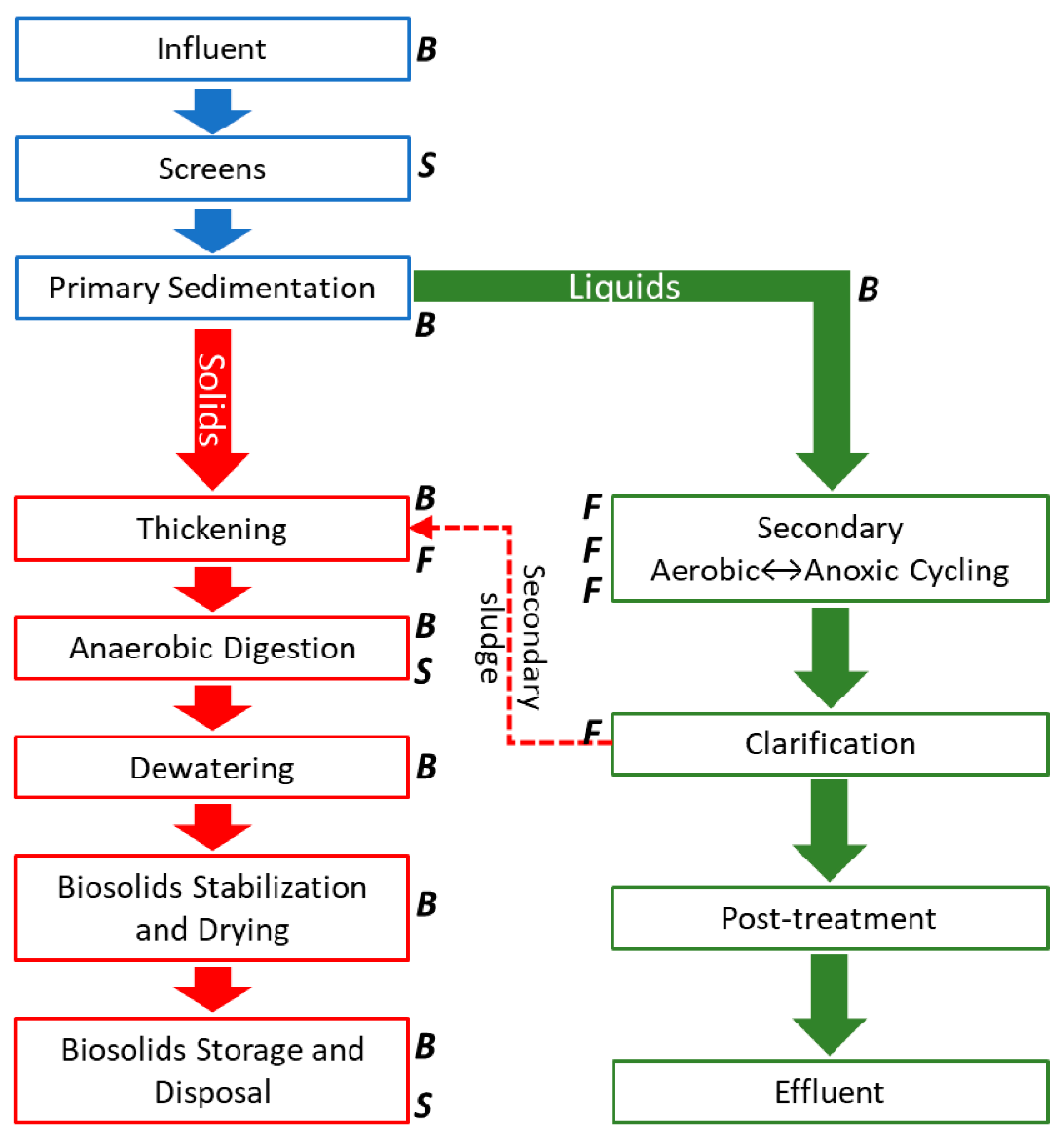
Modern WWTPs involve multistep waste processing [1,2]. First, the influent is screened for objects greater than a few millimeters diameter; these screenings and grit are collected and then sent to landfill. The screened influent undergoes primary treatment through sedimentation. Solids are passed to secondary solids treatment, while the supernatant liquid is pumped to reactor-clarifiers. Solids undergo various thickening processes (e.g., through gravity thickener belts and centrifugation), stabilization (e.g., with lime), and finally re-use or disposal. Meanwhile, secondary water treatment process involves wastewater passing through multiple aerobic and anaerobic cycles containing activated sludge prior to clarification, disinfection and discharge. Due to each process releasing various mixtures of odorants as different components break down at various stages, concentrations of odorous compounds and their observed overall offensiveness can differ significantly. Further impeding prediction of odor are factors such as influent composition and weather conditions. Complicating generalization across plants are different processing approaches and climate effects. Odorous gas emitted at each stage is commonly passed through biofilters or bio-scrubbers. Therefore, odor emission rates at each point are not indicative of raw odor generated at this stage of the process but are an indication of treated odorous gas.

Despite the process complexities, hydrogen sulfide has consistently been used in the industry as an indicator of odor [1]. Low-to-medium cost sensors have been utilized widely to monitor hydrogen sulfide for this purpose [3]. However, other odorous species are also usually present and can have lower odor thresholds than hydrogen sulfide [4]; for example, methyl mercaptan. The biosolids containment shed has consistently displayed high odors when measured with olfactometry, while low levels of hydrogen sulfide have been detected from ambient air at this site on numerous occasions (< 10 ppbV) (operational data from internal study at plant, current SIFT-MS data from this study). Hydrogen sulfide as an indicator has its challenges as it is not always present in odorous environments and the correlation of hydrogen sulfide with odor is inconsistent [5,6]. More sophisticated measurement techniques are required to better represent complex odor from complex wastewater processes.

Odor analysis using sensor technologies has proved challenging. ENoses (or technical sensors) received significant attention in the late 1990s and 2000s [1] as a solution to modelling and predicting complex odor. These devices still do not qualify as equivalent to human noses for olfactometry measurements [7]. Conventional laboratory analysis of odors using chromatographic methods can be expensive due to the need for multiple analyses for the chemically diverse odor species (ranging from reduced sulfur compounds, to amines, to aldehydes, to volatile fatty acids). Furthermore, laboratory analysis is limited to grab samples due to this complexity and the nature of the conventional chromatographic instrumentation. Hence, modelling complex changes in odor over time is extremely challenging.

Since the late 2000s, direct mass spectrometry (DMS) techniques have become more mainstream in environmental monitoring [8] and identification of odors in food sciences [9]. DMS methods can analyze odor in real-time and can be deployed at site. Proton transfer reaction mass spectrometry (PTR-MS) has been the most widely applied DMS technique for environmental monitoring [10,11,12,13,14]. PTR-MS has specifically been used to optimize effluent control biofiltration systems at an intensive pig production facility using static and mobile laboratory methods [15,16].

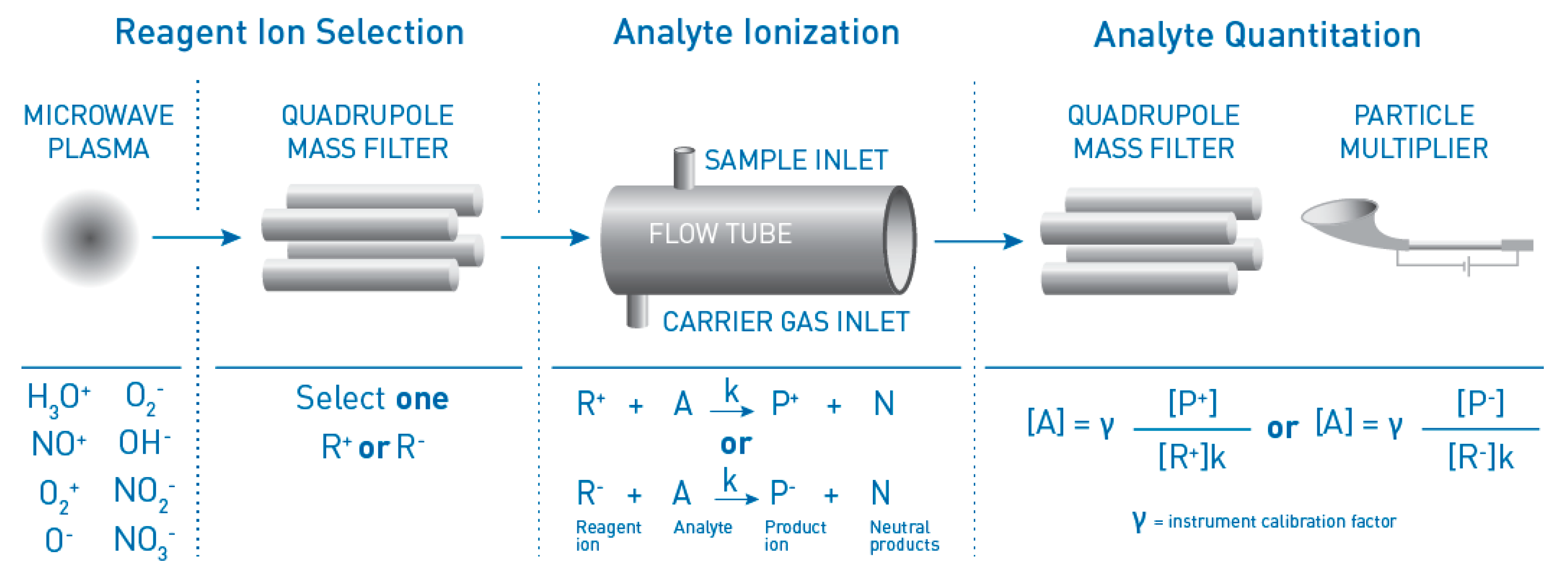
Selected ion flow tube mass spectrometry (SIFT-MS) was commercialized by Syft Technologies more recently than PTR-MS. SIFT-MS (Figure 1) has a potential advantage over PTR-MS due to its multiple, rapidly switchable chemical ionization agents (so called reagent or precursor ions) that detect diverse odor compounds with high selectivity [15,17,18,19]. The SIFT-MS technique has been described in detail elsewhere [20,21]. Briefly, the SIFT-MS reagent ions are generated by a microwave plasma through moist air, then selected individually using a quadrupole mass filter. The mass-selected reagent ions first encounter carrier gas, which collisionally cools the ions and contributes to consistent ionization and quantitation from reagent ion-analyte reactions occurring when the sample is introduced. After a few milliseconds of reaction, remaining reagent ions and product ions are mass-filtered and detected, with concentrations calculated point-by-point. Data obtained by SIFT-MS instruments are congruent with an accepted chromatographic method for environmental volatile organic compound (VOC) analysis [22].

Braithwaite’s review of the odor analysis literature [5] has noted the potential of SIFT-MS for odor analysis in parallel with gas chromatography-mass spectrometry/olfactometry (GC-MS/O) and sensory analysis (the odor profile method (OPM) in particular). GC-MS/O separates volatile compounds via gas chromatography, determines their mass by mass spectrometry and evaluates their odor strength and characterization via sensory evaluation (olfactometry) [23,24]. In addition to the complexities of chemical odorant species detection, the chemical, physiological and neurological mechanisms involved in odor perception in humans are complex and yet to be fully understood. Of the > 1000 known genes encoding olfactory receptors in the human genome (the largest multigene family), most are found in gene clusters and only 388 of these may be functional [25]. This may be due to coding region disruptions that may create non-functional pseudogenes [25,26]. A comparison of 20 receptor genes from human to chimpanzees showed the loss of function on half of the chosen receptors in humans when compared to the functioning gene in chimpanzees [26]. Genetic variation between family members has been studied and a hereditary link was found between the linkage of pleasantness to cinnamon odors and the perceived intensity of chocolate, rose and paint thinner [27]. Therefore, it is probable that genetic variation within humans plays a role in odor assessment and perceived intensity of individual odors.

When attempting to generate algorithms that replicate odor receptor responses, there is no linear correlation between sensory input and odor mapping in the brain. For example, a single odor receptor such as hOR1G1 can recognize a large spectrum of odors that stimulate many different olfactophores in the olfactory bulb [28]. This receptor was also suggested to have differing affinity to different odorants at its receptor binding site inferring that in a complex mix, some odorants would have preferential binding due to their affinity to the binding site. It was also suggested that binding was easily reversible due to the hydrogen binding associated with the binding site [28]. Much work is needed before the physiological workings of each receptor expressed at any one time in any of the millions of olfactory sensory neurons present in human noses is fully understood. In addition, each olfactory sensory neuron has a three-month life span and is regenerated over the human lifetime. A negative feedback loop is used to ensure only one type of olfactory receptor is ever expressed in a cell at one time [29]. Hence, with this complexity and variation between individuals, it is difficult to generate standard algorithms to predict odor responses of much of the human population.

This paper seeks to bridge the gap between sensory and instrumental methods in a way that has not been previously possible because of the limitations of conventional instrumental techniques. It first describes the first application of SIFT-MS to identify probable odor-causing chemical species at a modern WWTP, evaluating its performance against the extant literature for chemical odorant analysis in WWTPs. Then a comparison is made of SIFT-MS against odor concentration from dynamic dilution olfactometry, and against informal odor notes. These evaluations were conducted alongside an existing biennial odor emissions survey at the WWTP. The results presented here indicate the correlation of chemical composition provided by SIFT-MS analysis to final odor emissions (post odor treatment) at different stages of the plant. However, this four-month study indicated that SIFT-MS could be developed into a useful tool to assist in making operational decisions regarding odor mitigation strategies and assist with planning for future odor mitigation infrastructure (i.e., developing most suitable bio-scrubber media suited to the site). SIFT-MS analysis may be used for continuous monitoring on site to assess the effect of operational changes on odor emissions from isolated parts of the plant. SIFT-MS analysis may also be used to monitor biogas composition and determine the efficiency of the siloxane scrubber that reduces organosilicon-based engine wear. SIFT-MS data may also assist with furthering the capability of wastewater treatment process modelling software as it can provide additional indicators of the changes to dominant biochemical pathways involved in processes. Further validation and modelling would be required before the technique could provide online feedback and alerts to assist with operational process optimization.

2. Materials and Methods

2.1. Wastewater Treatment Plant and Sampling Design

The modern New Zealand WWTP investigated in this study treats wastewater from both industrial and residential sources. The odor survey was conducted over the Southern Hemisphere summer and early autumn/fall period (December 2018–April 2019) and focused on odor emission sources post-treatment at the plant using olfactometry analysis. Parallel samples were collected for SIFT-MS chemical analysis in the same material (nalophan bag). Samples for comparative analysis were obtained from a wide range of potential odor sources at the plant including odor beds and reactor clarifiers. Figure 2 shows a schematic diagram of the WWTP process. Raw sewage (influent) was screened for debris and grit, then processed via primary sedimentation. The liquid was pumped for treatment in the secondary liquids activated sludge process, where the process included repeated aerobic and anaerobic cycling prior to clarification and sterilization. The solids were passed to the secondary solids process, in which thickening, anaerobic digestion, dewatering and stabilization steps were undertaken prior to disposal of the biosolids. The biogas generated during anaerobic digestion was combusted for energy generation.

Table 1. Process locations for biofilters that were sampled in this study (using the flux chamber approach according to AS/NZS 4323.4:2009) and biofilter compositions.

Treatment Phase	Location(s)	Location ID	Number of Samples	Biofilter Type 1
Influent and Primary	Screens, Primary tanks	IP-EF	13	A
Primary	Pumping station	P-PS	2	A
Primary	Splitter box for Reactor-Clarifiers	P-SP	6	A, B, C
Secondary solids	Gravity thickeners	SS-GT	5	D
Secondary solids	Digester Feed	SS-DF	3	A
Secondary solids	Centrifuge	SS-CE	3	A
Secondary solids	Biosolids storage	SS-BS	10	A
Secondary solids	Ammonia scrubber	SS-AS	4	D
Total samples			46

¹ Biofilter types: A = 70% Scoria (AP7), 30% Aged Bark; B = 37% Coarse Scoria (50/20 mm), 37% Fine Scoria (20/7 mm), 26% Compost/Pumice Mix (50-50 Standard Compost & 1–3 mm Pumice; C = Bark, Compost/Pumice mix; D = 37% Coarse Scoria (50/20 mm), 37% Fine Scoria (20/7 mm), 26% Compost/Pumice Mix (50-50 Standard Compost & 1–3 mm Pumice).

,

Table 2. Process locations for flotation samples that were collected during this study (using the flux chamber approach according to AS/NZS 4323.4:2009 [30]).

Treatment Phase	Location(s)	Location ID	Number of Samples
Secondary water	Reactor aerobic location 1	SW-A1	8
Secondary water	Reactor aerobic location 2	SW-A2	9
Secondary water	Reactor anoxic location 1	SW-AO	9
Secondary water	Clarifier	SW-CL	20
Secondary solids	Dissolved air flotation	SS-AF	6
Total samples			52

and

Table 3. Process locations for stack and ambient samples collected during this study (according to AS/NZS 4323.3:2001 [31]).

Treatment Phase	Location(s)	Location ID	Number of Samples	Sample Type
Influent-Primary	Screens building	IP-SB	2	Ambient bag
Secondary solids	Gas turbine stack, post biogas combustion	SS-TS	3	Stack bag via port
Secondary solids	Sludge stack, biosolids building	SS-SS	4	Stack bag via port
Total samples			9

summarize the process locations corresponding to sampling using flux chambers on biofilters, flotation chambers on liquid surfaces, and stack/ambient gases, respectively. These tables also introduce a four-letter code that is used to identify locations in abbreviated form in subsequent text, tables, and figures (the “Location ID”; e.g., IP-EF for the earth filters on the screens in the influent/primary treatment phase).

Figure 2. Schematic diagram of the process at the WWTP investigated in this study. Sampling method (Table 2, Table 3 and

Table 4. Target compounds for SIFT-MS analysis, together with published odor detection thresholds (ODTs) and odor notes. Reagent ions and primary product ions mass-to charge ratios (in Daltons) used to quantify target compounds, with secondary (water cluster) ions shown in parentheses. To avoid unnecessary complications, not all ion products of each volatile are shown. More details are given in the text.

Compound	Sensory				SIFT-MS 1
	ODT/ppbV @ 25 °C	Ref. 2	Odor Note	Ref. 3	H3O+	NO+	O2+	Ref. 4	LOQ/ppbV
Sulfur-containing
Hydrogen sulfide	0.41	1	Rotten eggs	I	35			A	0.3
Methyl mercaptan	0.071	1	Decayed cabbage, rotten garlic, sulfur, sweaty	I, II	49		48	A	0.3
Dimethyl sulfide + ethyl mercaptan	3.0	1	Decayed vegetables/cabbage, seaweed, garlic	I, II	63	62	62	B	0.5
Dimethyl disulfide	2.2	1	Putrification, rotting seaweed, egg	I, II	95	94	94	B	0.2
Dimethyl trisulfide	1.5	1	Rotten cabbage / vegetables, onions	II	127	126	126	C	0.5
Allyl methyl sulfide	6.1	2	Bad breath, acrid sweat	II	89		88	D	1.6
Diethyl disulfide	0.024	1	Gassy, ripe onion, greasy, garlic	III	123	122		E	0.5
Carbon disulfide	210	1	Sweet, decayed vegetables	II			76	E	7.9
Propyl mercaptans	0.51	3	Unpleasant	I		76		A, E	0.5
Butyl mercaptans	0.81	4	Unpleasant	I	91	90		E	0.4
Nitrogen-containing
Ammonia	1600	1	Sharp, pungent	I	18 (36)		17 (18, 35, 36)	F	10.1
Methylamine	36	1	Fishy	I		31		G	1.6
Dimethylamine	32	1	Fishy	I	46			F	11.2
Trimethylamine	2.4	5	Fishy, ammoniacal	I	60	59		F	2.3
Diethylamine	47	1	Fishy, ammoniacal	III	74			F	7.6
Triethylamine	5.3	1	Fishy, ammoniacal	III	102	101		F	0.2
Isopropylamine	25	1	Fishy, ammoniacal	III		44		F	3.5
Putrescine	2.8	6	Decomposing meat	I	71	69, 99		D	2.0
Cadaverine	2.4	7	Decomposing meat	I		87	88	D	1.3
Indole	0.29	1	Faecal, nauseating	I	118	117	117	H	0.2
Skatole	0.093	8	Faecal, nauseating	I	132	131	131	H	0.2
Pyridine	62	1	Disagreeable, irritating	I	80	109	79	F	0.2
Volatile fatty acids
Acetic acid	6.1	1	Vinegar, acrid, plastic	I, II	61 (79)	90		I	1.9
Butyric acid	0.19	1	Rancid, sweaty, chemical, green	I, II	89 (107)	118		I, J	0.6
Valeric acid	0.038	1	Sweaty	I	103			E	0.8
Aldehydes
Formaldehyde	490	1	Acrid, suffocating	I	31			K	6.6
Acetaldehyde	50	5	Fruit, apple	I	45 (63)	43 (61)		K	21.6
Propanal	5.9	9	Sweet, ester	IV		57		K	2.3
Butanal isomers	0.34	1	Rancid, sweaty + Fruit	I		71		K, L	1.1
Pentanal isomers	0.45	9	Almonds, pungent (pentanal)	II		85		L, M	0.4
Hexanal	0.83	10	Grass	II	83, 101 (119)	99		K	1.1
Heptanal	56	11	Fresh, green, herbal	III	115 (133)	113	96	L	0.5
Nonanal	40	12	Citrus, rose	II	143 (161)	141	124	N	0.9
Decanal	9.9	10	Soap, citrus, baking bread, yeast, peanuts, burning	II	157 (175)	155		L	0.5
Benzaldehyde	140	10	Almonds, bitter, musty, mushrooms	II	107	105		K	0.5
Heptadienal	13	13	Green, pungent, fatty	III	109			O	0.5
Decadienal	0.026	14	Citrus, fatty, oily, green, chicken	III		151	81	L	0.5
Ketones
Acetone	42,500	1	Fruit, sweet	I		88		K	4.6
Butanone	440	1	Green apple, sweet, acetone-like	I, II		102		K	0.2
Pentanone isomers	99	15	Acetone-like, fruit	II		116		K	0.5
Methyl isobutyl ketone	170	1	Sweet, acetone-like, minty	II		130		P	0.5
Heptanone isomers	6.9	1	Soap	II		144		Q	0.5
2,3-Butanedione	0.051	1	Butter	V		86		J, K	0.6
Alcohols
Ethanol	530	1	Sweet	V	47 (65)	45 (63)		R	68.5
Propanol isomers	26,000	1	Sharp musty	II	43	59		R	2.1
Butanol isomers	220	1	Alcoholic, sweet, banana	II		73		R	4.0
Cresol isomers	0.090	1	Medicinal, urine, piggery, faecal/floral	II		108	108	S	0.2
2-Methylisoborneol	0.0070	16	Musty water, earthy	II	151			T	0.5
Geosmin	0.0070	1	Musty water, earthy	II	165			O	0.5
Monoterpenes and derivatives
Monoterpenes	32	1	Diverse odors; generally natural/fresh	II		136	136	U	0.5
Carvone	5.5	17	Mint, musty, oily	II		180		V	0.5
Dihydrocarvone	170	18	Herb, mint, hospital, sweet, wood, mushrooms	II	153	182	152	W	0.5
Thymol	6.5	19	Thyme, aromatic, herbaceous, chemical, lemongrass	II		150		X	0.5
Hydrocarbons
Toluene	340	1	Rubber, musty, sweet, oily, solvent, gasoline	II	93	92	92	Y	0.6
Ethylbenzene + total xylene isomers	170	1	Sweet, aromatic	II	107	106		Y	0.6
C3-Alkylbenzenes	170	1	Aromatic, sweet	II		120	120	Y	0.5
C4-Alkylbenzenes (from diethylbenzene)	9.5	1	Solvent, rubber, musty, oily	II		134	119	O	0.5
Decane	620	1	Gasoline	II		141	142	O	0.7
Undecane	880	1	Gasoline	II		155	156	O	0.5
Dodecane	110	1	Gasoline	II		169		O	5.1
Chlorine-containing
Dichlorobenzene	120	20	Pleasant, aromatic	VI	147	146	146	D, N	0.5
Chlorophenol isomers	0.19	21	Medicinal	VII	129		128, 130	O	0.5

¹ SIFT-MS detection m/z for reagent ions are shown in Daltons. ² ODT references: see Supplementary Data—Table 4 References. ³ Odor note references: see Supplementary Data—Table 4 References. ⁴ SIFT-MS library data references: see Supplementary Data—Table 4 References.

) is indicated as B = biofilter, F = flotation and S = stack/ambient.

Figure 2. Schematic diagram of the process at the WWTP investigated in this study. Sampling method (Table 2, Table 3 and Table 4) is indicated as B = biofilter, F = flotation and S = stack/ambient.

2.2. Sampling Procedures

Sampling was carried out on liquid surfaces (i.e., dissolved air flotation (DAF) tanks in secondary solids treatment and reactor clarifier tanks in secondary water treatment) using a United States Environmental Protection Agency (US EPA) static flux chamber (SFC) to undertake the monitoring [32]. For sources with positive gas release (i.e., the biofilter outlets) an open hood sampling method was used. In both cases, sampling was in conformance with procedures described in AS/NZS 4323.4:2009 [30].

Engine stack and sludge handling stack samples were collected using a point source emission sampling method as described in AS/NZS 4323.3:2009—Stationary Source Emissions Part 3: Determination of Odor Concentration by Dynamic Olfactometry [31].

In all cases, Nalophan NA odor bags (made in house from film supplied by Coimex International Limited, Brazil) were used to contain air samples for both olfactometry and instrumental analysis. Sampling lines were made from PTFE tubing and used once. Each collection apparatus was placed and left to condition prior to collecting samples. Collection of samples was via a lung system where a vacuum was applied to the sample barrel resulting in the bag ‘lung’ filling with sample air without contamination from the pump. Bags were filled with sample, conditioned and emptied. The conditioned bags were then filled with sample for analysis using gas-sampling pumps with calibrated flows [30].

Samples for both sensory and instrumental analysis were analyzed within 24 h of sampling.

2.3. Sensory Analysis

Olfactometry was conducted at the Watercare Laboratory Services Odor Laboratory. Odor concentrations (in odor units m⁻³; OU m⁻³) were determined using dilution olfactometry according to AS/NZS 4323.3:2001 [31]. An Olfasense olfactometer (Kiel, Germany, www.to-evolution.com) was used with four to six panelists.

Assessment of odor character was conducted informally according to an in-house laboratory procedure. The odor characteristic is a qualitative measurement of what is predominantly perceived by the odor panelists. After dilution olfactometry is completed, the sample is presented to all odor panelists to carefully sniff the undiluted sample. The panel must reach a consensus on the predominant odor character and its intensity. An odor character description is provided to the technician for each sample and the panel are not informed of the source of the odor.

2.4. SIFT-MS

SIFT-MS data for this article were obtained using a Voice200ultra SIFT-MS instrument (Syft Technologies, Christchurch, New Zealand; www.syft.com) in positive ion mode. Target compounds for SIFT-MS analysis were derived from References [1], [2] and [4]. The reagent-product ion pairs for SIFT-MS detection of each target compound are summarized in Table 4. Other SIFT-MS product ions were usually available but as they were not utilized in determining the final concentrations, they have been omitted for clarity.

Quantitation for most compounds was carried out from the SIFT-MS library [22]. Hydrogen sulfide, methyl mercaptan and ethyl mercaptan + dimethylsulfide, and dimethyl disulfide were calibrated against certified gas mixtures (CAC Gas, Sydney, Australia) to improve accuracy. Limits of quantitation (LOQs) were estimated as one-half the mean blank concentration. Due to sampling from bags, minimum values for LOQs were set at 0.2 parts-per-billion by volume (ppbV) for targeted compounds (selected ion mode, SIM) and 0.5 ppbV for compounds processed subsequently from full scan data. LOQs are shown in Table 4. Blank bags were filled with odor-free scrubbed air used in olfactometry and provided a baseline of contamination from the sampling method.

To facilitate comparison of the SIFT-MS data with the sensory results, concentrations were converted to odor activity values (OAVs), by dividing the concentration measurement by the odor detection threshold (ODT). Table 4 summarizes ODT concentrations [33] and odor notes for target compounds, where these are known. Wherever possible ODTs were derived from Nagata [34]. However, where data from Nagata [34] were missing, or were at significant variance compared with other post-1970 values, an alternative recent source was utilized. Where isomers or isobaric compounds cannot be resolved with SIFT-MS and are expected in samples, values for all were compared and a representative mid-range value was utilized (e.g., for the monoterpenes, β-pinene). However, it should be noted that for many compounds their published ODTs do vary considerably, so OAVs are viewed as indicative.

3. Results

Table 5. Sensory data and SIFT-MS concentration data (in ppbV) for odor sources from influent and primary treatment. The range of values for each source is shown. See the text and table footnotes for more details.

	ODT/ppbV at 25 °C	Instrument LOQ/ppbV	Odor Sources 1
			Screens, Primary Tanks, IP-EF	Screens Building, IP-SB	Pumping Station, P-PS	Splitter Box for Reactor-Clarifiers, P-SP
Sample type			Biofilter	Ambient	Biofilter	Biofilter
Number of samples			13	2	2	6
Olfactometry
Concentration 2			65–41,086	143–191	44–207	55–4858
Intensity 3			I, VL, L, M, S	I, VL	I, VL	VL, L, M
Character 4			V, Se, E, I, R, C	I, V	I, V	V, C, Se, R
Odorants 5
Sulfur-containing
Hydrogen sulfide	0.41	0.3	<LOQ–3800	4.2–4.4	<LOQ–10	1.5–130
Methyl mercaptan	0.071	0.3	<LOQ–130	0.5–1.4	0.6–0.7	1.1–86
Dimethyl sulfide + ethyl mercaptan	3.0	0.5	<LOQ–7.9 [2]	<LOQ	<LOQ	<LOQ–27
Dimethyl disulfide	2.2	0.2	<LOQ–2.5 [4]	<LOQ	<LOQ–0.6	<LOQ–30
Dimethyl trisulfide	1.5	0.5	<LOQ–15 [5]	<LOQ–0.6	<LOQ–0.8	<LOQ–6.9
Allyl methyl sulfide	6.1	1.6	<LOQ–4.6 [2]	<LOQ	<LOQ	<LOQ–5.9
Diethyl disulfide	0.024	0.5	<LOQ–1.1 [1]	<LOQ	<LOQ–0.6	<LOQ–0.7 [1]
Carbon disulfide	210	7.9	<LOQ–13 [1]	<LOQ–10.8	<LOQ	<LOQ–73
Propyl mercaptans	0.51	0.5	<LOQ–4.1 [4]	<LOQ–0.9	<LOQ	<LOQ–3.8
Butyl mercaptans	0.81	0.4	<LOQ–1.5 [3]	<LOQ	<LOQ–0.6	<LOQ–1.9
Nitrogen-containing
Ammonia	1600	10.1	<LOQ–15 [2]	<LOQ	<LOQ	<LOQ
Methylamine	36	1.6	<LOQ–2.9 [1]	<LOQ	<LOQ	<LOQ–3.4
Dimethylamine	32	11.2	<LOQ	<LOQ	<LOQ	<LOQ
Trimethylamine	2.4	2.3	<LOQ	3.8–7.5	<LOQ	<LOQ–4.1 [2]
Diethylamine	47	7.6	<LOQ	<LOQ	<LOQ	<LOQ
Triethylamine	5.3	0.2	<LOQ–0.5 [3]	<LOQ	<LOQ–0.5	<LOQ–0.5 [2]
Isopropylamine	25	3.5	<LOQ	<LOQ–3.9	<LOQ	<LOQ
Putrescine	2.8	2.0	<LOQ–72 [4]	<LOQ	<LOQ–5.7	<LOQ–78
Cadaverine	2.4	1.3	<LOQ	<LOQ	<LOQ	<LOQ–2.8 [1]
Indole	0.29	0.2	<LOQ–0.3 [1]	<LOQ	<LOQ	<LOQ
Skatole	0.093	0.2	<LOQ	<LOQ	<LOQ	<LOQ–0.5 [1]
Pyridine	62	0.2	<LOQ	<LOQ	<LOQ	<LOQ
Volatile fatty acids
Acetic acid	6.1	1.9	<LOQ	<LOQ	<LOQ	<LOQ–2.0 [1]
Butyric acid	0.19	0.6	<LOQ–1.1 [2]	<LOQ	<LOQ	<LOQ
Valeric acid	0.038	0.8	<LOQ–18 [5]	<LOQ–0.8	<LOQ–1.2	0.9–17
Aldehydes
Formaldehyde	490	6.6	<LOQ–37 [4]	<LOQ	<LOQ–14	<LOQ–24
Acetaldehyde	50	21.6	<LOQ–160 [6]	<LOQ	<LOQ–25	37–96
Propanal	5.9	2.3	<LOQ–29 [1]	<LOQ	<LOQ–2.4	<LOQ–8.2
Butanal isomers	0.34	1.1	<LOQ–17 [2]	<LOQ	<LOQ	1.6–11
Pentanal isomers	0.45	0.4	<LOQ–2.9 [4]	<LOQ	<LOQ–0.5	0.5–1.0
Hexanal	0.83	1.1	<LOQ–7.8 [3]	1.4–2.0	<LOQ–1.6	<LOQ–3.2
Heptanal	56	0.5	<LOQ–9.2 [2]	<LOQ–0.9	<LOQ	<LOQ–6.8
Nonanal	40	0.9	<LOQ–4.4	<LOQ	<LOQ–2.0	<LOQ–1.2
Decanal	9.9	0.5	<LOQ–3.6 [4]	<LOQ–1.4	<LOQ–0.9	<LOQ–1.8
Benzaldehyde	140	0.5	<LOQ	<LOQ	<LOQ	<LOQ–0.5 [1]
Heptadienal	13	0.5	<LOQ–12 [4]	<LOQ	<LOQ–1.0	<LOQ–13
Decadienal	0.026	0.5	<LOQ–7.1 [1]	<LOQ	<LOQ	<LOQ–5.4 [2]
Ketones
Acetone	42,500	4.6	<LOQ–14 [2]	<LOQ	<LOQ	<LOQ
Butanone	440	0.2	<LOQ–2.9 [3]	<LOQ	<LOQ–1.2	<LOQ–0.7
Pentanone isomers	99	0.5	<LOQ	<LOQ	<LOQ	<LOQ
Methyl isobutyl ketone	170	0.5	<LOQ–0.9 [1]	<LOQ	<LOQ–0.7	<LOQ–1.1 [1]
Heptanone isomers	6.9	0.5	<LOQ	<LOQ	<LOQ	<LOQ
2,3-Butadione	0.051	0.6	<LOQ–8.2 [1]	<LOQ	<LOQ–0.6	<LOQ–4.4
Alcohols
Ethanol	530	68.5	<LOQ–118 [3]	470–630	<LOQ	<LOQ–580
Propanol isomers	26,000	2.1	<LOQ–0.6 [2]	2.9–3.5	<LOQ–4.1	<LOQ–1.5 [2]
Butanol isomers	220	4.0	<LOQ–6.0 [5]	<LOQ–2.5	<LOQ–5.4	1.1–4.6
Cresol isomers	0.090	0.2	<LOQ–0.4 [2]	<LOQ–0.2	<LOQ–0.3	<LOQ–0.5
2-Methylisoborneol	0.0070	0.5	<LOQ–4.7 [2]	<LOQ–1.2	<LOQ	<LOQ–3.2 [2]
Geosmin	0.0070	0.5	<LOQ–4.5 [6]	<LOQ–1.0	<LOQ–0.5	1.3–5.6
Monoterpenes and derivatives
Monoterpenes	32	0.5	<LOQ–17 [6]	0.6–1.5	<LOQ	<LOQ–50
Carvone	5.5	0.5	<LOQ–0.6 [1]	<LOQ	<LOQ	<LOQ–0.7 [1]
Dihydrocarvone	170	0.5	<LOQ–2.6 [5]	<LOQ	<LOQ–0.7	<LOQ–2.3
Thymol	6.5	0.5	<LOQ–1.4 [4]	<LOQ	<LOQ	<LOQ–1.1
Hydrocarbons
Toluene	340	0.6	<LOQ–48 [3]	1.8	<LOQ–1.7	<LOQ–900
Ethylbenzene + total xylene isomers	170	0.6	<LOQ–42 [3]	<LOQ	<LOQ–0.7	<LOQ–28
C3-Alkylbenzenes	170	0.5	<LOQ–12 [1]	<LOQ	<LOQ	<LOQ–12
C4-Alkylbenzenes	9.5	0.5	<LOQ–8.7 [1]	<LOQ	<LOQ	<LOQ–6.2 [2]
Decane	620	0.7	<LOQ–9.5	1.5	<LOQ–1.9	<LOQ–7.6
Undecane	880	0.5	<LOQ–11 [3]	<LOQ–0.6	<LOQ–0.8	<LOQ–1.0
Dodecane	110	5.1	<LOQ–34 [1]	<LOQ	<LOQ	<LOQ–23 [1]
Chlorine-containing
Dichlorobenzene	120	0.5	<LOQ–1.3 [1]	<LOQ	<LOQ	<LOQ–1.7 [1]
Chlorophenol isomers	0.19	0.5	<LOQ–1.5 [1]	<LOQ	<LOQ	<LOQ–2.2 [2]

¹ For the SIFT-MS data, where less than 50% of samples report above the LOQ for a compound, the number of measurements greater than the LOQ is shown in square brackets after the concentration range. ² Odor concentration is in OU m⁻³. ³ Odor intensity range, with most frequent in bold. Abbreviations: I = indiscernible, VL = very light, L = light, M = moderate, S = strong. ⁴ Odor characters in order of high to low frequency. Abbreviations: C = chemical, E = earth, F = rotten fish, I = indiscernible, M = musty, R = rotten vegetation, Se = sewage, V = vegetation. ⁵ Detected using SIFT-MS and converted to OAVs in ppbV, as described in the text.

,

Table 6. Sensory data and SIFT-MS concentration data (in ppbV) for odor sources from secondary liquids treatment. The range of values for each source is shown. See the text and table footnotes for more details.

	ODT/ppbV at 25 °C	Instrument LOQ/ppbV	Odor Sources 1
			Reactor Aerobic–Location 1, SW-A1	Reactor Aerobic–Location 2, SW-A2	Reactor Anoxic–Location 1, SW-AO	Clarifier, SW-CL
Sample type			Flotation	Flotation	Flotation	Flotation
Number of samples			8	9	9	20
Olfactometry
Concentration 2			1551–50,370	158–712	210–890	155–655
Intensity 3			M, S	VL, L, M	L, M	VL, L, M
Character 4			Se, E, V	E, V, C	C, V	V, E
Odorants 5
Sulfur-containing
Hydrogen sulfide	0.41	0.3	46–2100	<LOQ–2.3	<LOQ–9.5	<LOQ–3.7
Methyl mercaptan	0.071	0.3	34–190	0.5–4.2	<LOQ–41	<LOQ–2.2
Dimethyl sulfide + ethyl mercaptan	3.0	0.5	2.9–9.3	<LOQ–2.8	<LOQ–6.1	<LOQ–2.7 [3]
Dimethyl disulfide	2.2	0.2	0.4–1.1	<LOQ–0.3	<LOQ–0.5	<LOQ–0.7 [9]
Dimethyl trisulfide	1.5	0.5	0.8–1.8	<LOQ—2.9	<LOQ–13	<LOQ–2.1 [8]
Allyl methyl sulfide	6.1	1.6	<LOQ–8.2	<LOQ–3.6 [2]	<LOQ–2.7 [3]	<LOQ–4.2 [9]
Diethyl disulfide	0.024	0.5	<LOQ–0.7 [1]	<LOQ	<LOQ	<LOQ–0.5 [1]
Carbon disulfide	210	7.9	<LOQ–14 [3]	<LOQ–9.1 [1]	<LOQ–9.8 [3]	<LOQ–11 [3]
Propyl mercaptans	0.51	0.5	0.7–3.9	<LOQ–0.8 [2]	<LOQ–1.1 [3]	<LOQ–0.8 [6]
Butyl mercaptans	0.81	0.4	1.1–1.4	<LOQ–0.9 [2]	<LOQ–1.1	<LOQ–1.0 [7]
Nitrogen-containing
Ammonia	1600	10.1	<LOQ–17	<LOQ–16 [2]	<LOQ–22 [2]	<LOQ–25 [2]
Methylamine	36	1.6	<LOQ–2.5 [2]	<LOQ–5.7 [2]	<LOQ	<LOQ–2.6 [4]
Dimethylamine	32	11.2	<LOQ	<LOQ	<LOQ	<LOQ
Trimethylamine	2.4	2.3	<LOQ–7.3 [3]	<LOQ–9.3 [3]	<LOQ–6.5 [3]	<LOQ–4.9 [5]
Diethylamine	47	7.6	<LOQ	<LOQ	<LOQ	<LOQ
Triethylamine	5.3	0.2	<LOQ–0.7	<LOQ	<LOQ–0.4 [3]	<LOQ–0.5 [8]
Isopropylamine	25	3.5	<LOQ	<LOQ–6.1 [3]	<LOQ–4.6 [2]	<LOQ–5.1 [3]
Putrescine	2.8	2.0	<LOQ	<LOQ–7.5	<LOQ–20	<LOQ–8.1
Cadaverine	2.4	1.3	<LOQ–8.3	<LOQ–1.6 [1]	<LOQ–2.6 [2]	<LOQ
Indole	0.29	0.2	<LOQ–2.6	<LOQ	<LOQ	<LOQ–0.3 [1]
Skatole	0.093	0.2	<LOQ	<LOQ	<LOQ	<LOQ
Pyridine	62	0.2	<LOQ	<LOQ–0.3 [1]	<LOQ	<LOQ–0.2 [2]
Volatile fatty acids
Acetic acid	6.1	1.9	<LOQ–2.5 [3]	<LOQ–2.2 [1]	<LOQ–5.3 [2]	<LOQ–3.6 [2]
Butyric acid	0.19	0.6	<LOQ–1.2	<LOQ–1.2 [2]	<LOQ–0.7 [3]	<LOQ–1.0 [7]
Valeric acid	0.038	0.8	1.9–3.6	<LOQ–2.5	<LOQ–7.8	<LOQ–2.6
Aldehydes
Formaldehyde	490	6.6	12–100	9–52	<LOQ–47	<LOQ–57
Acetaldehyde	50	21.6	82–310	<LOQ–140	<LOQ–120	<LOQ–223
Propanal	5.9	2.3	<LOQ–3.0 [1]	<LOQ–4.1 [1]	<LOQ–12	<LOQ–3.3 [1]
Butanal isomers	0.34	1.1	<LOQ–2.2	<LOQ–3.4 [4]	<LOQ–5.5	<LOQ–3.0 [9]
Pentanal isomers	0.45	0.4	0.9–1.9	<LOQ–0.8	0.7–2.3	<LOQ–1.4
Hexanal	0.83	1.1	1.2–3.4	<LOQ–2.5	1.4–5.0	<LOQ–2.1
Heptanal	56	0.5	<LOQ–1.0	<LOQ–1.9	<LOQ–6.0	<LOQ–1.1 [3]
Nonanal	40	0.9	<LOQ–8.5	<LOQ–2.3 [4]	<LOQ–2.3 [3]	<LOQ–3.3
Decanal	9.9	0.5	0.6–3.4	<LOQ–3.0	<LOQ–3.3	<LOQ–1.7 [7]
Benzaldehyde	140	0.5	<LOQ–1.6 [2]	<LOQ	<LOQ	<LOQ–1.3 [2]
Heptadienal	13	0.5	<LOQ–1.5 [2]	<LOQ–2.9 [4]	<LOQ–10.4	<LOQ–2.1 [8]
Decadienal	0.026	0.5	<LOQ	<LOQ–2.9 [3]	<LOQ–7.9	<LOQ–1.1 [1]
Ketones
Acetone	42500	4.6	10–31	<LOQ–8.2 [2]	<LOQ–16	<LOQ–1200 [7]
Butanone	440	0.2	0.7–1.4	<LOQ–0.6 [4]	<LOQ–1.6	<LOQ–1.4 [9]
Pentanone isomers	99	0.5	<LOQ	<LOQ	<LOQ–2.1 [3]	<LOQ
Methyl isobutyl ketone	170	0.5	<LOQ–8.3	<LOQ–0.7 [2]	<LOQ–0.9 [3]	<LOQ–0.8 [5]
Heptanone isomers	6.9	0.5	<LOQ	<LOQ	<LOQ	<LOQ
2,3-Butadione	0.051	0.6	<LOQ–1.6	<LOQ–0.8 [2]	<LOQ–4.9	<LOQ–0.9 [4]
Alcohols
Ethanol	530	68.5	<LOQ–250	<LOQ–2200 [3]	<LOQ–420 [4]	<LOQ–940 [7]
Propanol isomers	26,000	2.1	<LOQ–9.3	<LOQ–11	<LOQ–15 [4]	<LOQ–4.1 [6]
Butanol isomers	220	4.0	3.3–7.7	<LOQ–4.4	<LOQ–5.3	<LOQ–7.6
Cresol isomers	0.090	0.2	<LOQ–1.1	<LOQ	<LOQ–0.4 [3]	<LOQ–0.9 [7]
2-Methylisoborneol	0.0070	0.5	<LOQ	<LOQ–4.9 [3]	<LOQ–22	<LOQ–1.5 [2]
Geosmin	0.0070	0.5	0.6–1.6	<LOQ–5.4	0.8–41	<LOQ–1.7
Monoterpenes and derivatives
Monoterpenes	32	0.5	<LOQ–2.8	<LOQ–2.6	0.8-8.9	<LOQ–1.6 [6]
Carvone	5.5	0.5	<LOQ	<LOQ–1.8	<LOQ–5.0	<LOQ–0.6 [1]
Dihydrocarvone	170	0.5	<LOQ–1.5	<LOQ–0.9 [1]	<LOQ–5.0	<LOQ–1.3 [9]
Thymol	6.5	0.5	<LOQ–1.0 [3]	<LOQ–1.1 [4]	<LOQ–3.7	<LOQ–1.4 [9]
Hydrocarbons
Toluene	340	0.6	0.8–170	<LOQ–2.0	<LOQ–2.5	<LOQ–2.1 [5]
Ethylbenzene + total xylene isomers	170	0.6	<LOQ–13	<LOQ–1.8 [4]	<LOQ–4.3	<LOQ–1.2 [4]
C3-Alkylbenzenes	170	0.5	<LOQ–2.2 [3]	<LOQ–0.9 [1]	<LOQ–5.4	<LOQ–1.0 [1]
C4-Alkylbenzenes	9.5	0.5	<LOQ–1.2 [2]	<LOQ–1.3 [1]	<LOQ–6.5	<LOQ–1.2 [1]
Decane	620	0.7	<LOQ–3.6	<LOQ–1.9 [1]	1.5–28	<LOQ–3.4 [8]
Undecane	880	0.5	<LOQ–0.9	<LOQ–2.0 [4]	<LOQ–32	<LOQ–3.4 [3]
Dodecane	110	5.1	<LOQ–8.8 [2]	<LOQ–9.9 [1]	<LOQ–160	<LOQ–10 [4]
Chlorine-containing
Dichlorobenzene	120	0.5	<LOQ	<LOQ	<LOQ–1.3 [1]	<LOQ
Chlorophenol isomers	0.19	0.5	<LOQ	<LOQ	<LOQ–1.6 [2]	<LOQ–1.4 [1]

¹ For the SIFT-MS data, where less than 50% of samples report above the LOQ for a compound, the number of measurements greater than the LOQ is shown in square brackets after the concentration range. ² Odor concentration is in OU m⁻³. ³ Odor intensity range, with most frequent in bold. Abbreviations: I = indiscernible, VL = very light, L = light, M = moderate, S = strong. ⁴ Odor characters in order of high to low frequency. Abbreviations: C = chemical, E = earth, F = rotten fish, I = indiscernible, M = musty, R = rotten vegetation, Se = sewage, V = vegetation. ⁵ Detected using SIFT-MS and converted to OAVs in ppbV, as described in the text.

and

Table 7. Sensory data and SIFT-MS concentration data (in ppbV) for odor sources from secondary solids treatment. The range of values for each source is shown. See the text and table footnotes for more details.

	ODT/ppbV at 25 °C	Inst. LOQ/ppbV	Odor Sources 1
			Gravity Thickeners, SS-GT	Dissolved Air Flotation, SS-AF	Digester Feed, SS-DF	Gas Turbine Stack, SS-TS 2	Centrifu., SS-CE	Biosolids Storage, SS-BS	Ammonia Scrubber, SS-AS	Sludge Stack, SS-SS
Sample type			Biofilter	Flotation	Biofilter	Stack	Biofilter	Biofilter	Biofilter	Stack
Number of samples			5	6	3	3	3	10	4	4
Olfactometry
Concentration 3			24-153	138-11205	107-157	570-4567	98-710	119-269	204-3661	301-3244
Intensity 4			I, L	L, M, S	VL, L	L, S	VL, L, S	VL, L	L, M	L, M, S
Character 5			I, Se, V	E, V, R, M, Se, C	V	C	C, E, V	V, E	E, V, R, C	Se, C, V, F
Odorants 6
Sulfur-containing
Hydrogen sulfide	0.41	0.3	<LOQ–3.4	<LOQ–0.7 [2]	1.4-7.1	1-2-3.9	<LOQ–1.4	<LOQ–3.1	<LOQ–13	1.0-34
Methyl mercaptan	0.071	0.3	<LOQ–1.3	<LOQ–160	0.5-0.8	0.9-1.6, *	0.4-2.0	<LOQ–1.7	1.2-2.4	<LOQ–8.2
Dimethyl sulfide + ethyl mercaptan	3.0	0.5	<LOQ–0.5 [1]	<LOQ–10 [2]	<LOQ–0.6	<LOQ, *	<LOQ–0.7 [1]	<LOQ–0.8 [2]	<LOQ–1.7	<LOQ
Dimethyl disulfide	2.2	0.2	<LOQ–0.5 [2]	<LOQ–7.7 [2]	<LOQ–0.3 [1]	<LOQ, *	<LOQ–0.4	<LOQ	<LOQ–1.2	<LOQ–1.7
Dimethyl trisulfide	1.5	0.5	<LOQ–1.1 [2]	<LOQ–2.1	<LOQ–1.2 [1]	<LOQ–0.3, [1]	<LOQ–0.9 [1]	<LOQ–0.6 [3]	<LOQ–1.8	<LOQ–0.8
Allyl methyl sulfide	6.1	1.6	<LOQ	<LOQ–2.3	<LOQ–2.5 [1]	<LOQ–2.3, *	<LOQ–1.8 [1]	<LOQ	<LOQ–2.2 [1]	<LOQ
Diethyl disulfide	0.024	0.5	<LOQ–0.5 [1]	<LOQ–1.0 [1]	<LOQ	<LOQ, *	<LOQ	<LOQ	<LOQ–0.7 [1]	<LOQ
Carbon disulfide	210	7.9	<LOQ–11.4 [1]	<LOQ–14 [1]	<LOQ	<LOQ, *	<LOQ	<LOQ	<LOQ	<LOQ
Propyl mercaptans	0.51	0.5	<LOQ–0.8 [2]	<LOQ–1.2 [1]	<LOQ	<LOQ, *	<LOQ–0.6 [1]	<LOQ–1.2	<LOQ–0.6 [1]	<LOQ–1.6
Butyl mercaptans	0.81	0.4	<LOQ–0.5 [1]	<LOQ–1.9 [2]	<LOQ–1.0 [1]	<LOQ–1.8, *	<LOQ–0.9	<LOQ–0.5 [3]	<LOQ–0.9	<LOQ
Nitrogen-containing
Ammonia	1600	10.1	<LOQ	<LOQ	<LOQ	<LOQ–12	11-16	<LOQ–15 [2]	<LOQ–3700 [1]	<LOQ–4700
Methylamine	36	1.6	<LOQ	<LOQ–1.8 [1]	<LOQ–1.6 [1]	<LOQ–5.3, *	<LOQ–1.8	<LOQ–3.5 [4]	<LOQ–3.0	<LOQ–4.7
Dimethylamine	32	11.2	<LOQ	<LOQ–20 [1]	<LOQ	<LOQ, *	<LOQ	<LOQ	<LOQ–26 [1]	<LOQ–11.9 [1]
Trimethylamine	2.4	2.3	<LOQ	<LOQ	<LOQ–2.9	<LOQ	<LOQ–6.4	<LOQ–38 [4]	<LOQ–4.8	<LOQ–30.1
Diethylamine	47	7.6	<LOQ	<LOQ	<LOQ	<LOQ, *	<LOQ	<LOQ	<LOQ–23 [1]	<LOQ–8.6 [1]
Triethylamine	5.3	0.2	<LOQ–0.3 [2]	<LOQ–0.2 [2]	<LOQ	<LOQ–1.5 [1]	<LOQ–0.3	<LOQ–0.2 [2]	<LOQ–0.3	<LOQ–0.2 [1]
Isopropylamine	25	3.5	<LOQ	<LOQ	<LOQ	<LOQ, *	<LOQ	<LOQ–4.6 [3]	<LOQ–76 [1]	<LOQ–79
Putrescine	2.8	2.0	<LOQ–7.3 [2]	<LOQ–2.4 [1]	<LOQ–5.5 [1]	<LOQ–2.1, *	2.7-3.9	<LOQ–2.6 [3]	<LOQ–11.2	<LOQ–2.1 [1]
Cadaverine	2.4	1.3	<LOQ	<LOQ–1.6 [1]	<LOQ	<LOQ, *	<LOQ	<LOQ	<LOQ	<LOQ
Indole	0.29	0.2	<LOQ	<LOQ	<LOQ	<LOQ–0.5 [1]	<LOQ	<LOQ	<LOQ	<LOQ
Skatole	0.093	0.2	<LOQ	<LOQ	<LOQ	<LOQ, *	<LOQ–0.2 [1]	<LOQ	<LOQ	<LOQ
Pyridine	62	0.2	<LOQ	<LOQ–1.6 [2]	<LOQ	<LOQ, *	<LOQ	<LOQ	<LOQ–0.2 [1]	<LOQ
Volatile fatty acids
Acetic acid	6.1	1.9	<LOQ	<LOQ–5.4 [1]	<LOQ–2.5 [1]	<LOQ–31	<LOQ–4.1	<LOQ–5.0	<LOQ	<LOQ–4.2
Butyric acid	0.19	0.6	<LOQ	<LOQ–0.8 [1]	<LOQ	<LOQ–1.3 [1]	<LOQ	<LOQ	<LOQ–0.6 [1]	<LOQ
Valeric acid	0.038	0.8	<LOQ–1.6 [2]	<LOQ–1.6 [2]	<LOQ–1.9	1.0-10.7	1.5-2.5	<LOQ–1.0	<LOQ–3.2	<LOQ
Aldehydes
Formaldehyde	490	6.6	<LOQ–23	<LOQ–110	19-28	37-4400	<LOQ–32	<LOQ–63	13-35	<LOQ–32
Acetaldehyde	50	21.6	<LOQ–83	<LOQ–100	55-128	<LOQ–1100	<LOQ–98	<LOQ–138	<LOQ–98	<LOQ–58
Propanal	5.9	2.3	<LOQ	<LOQ	<LOQ	19-124	<LOQ	<LOQ	<LOQ	<LOQ–3 [1]
Butanal isomers	0.34	1.1	<LOQ–1.4 [1]	<LOQ–1.3 [1]	<LOQ	<LOQ–16	<LOQ–2.6	<LOQ–2.4	<LOQ–3.2	<LOQ–1.6 [1]
Pentanal isomers	0.45	0.4	<LOQ–0.8 [2]	<LOQ–0.7 [2]	<LOQ–0.9	0.8-8.5	0.7-0.9	<LOQ–0.7 [4]	<LOQ–1.5	<LOQ–0.4 [1]
Hexanal	0.83	1.1	<LOQ–1.9 [1]	<LOQ–2.0	<LOQ–1.9 [1]	<LOQ–6.8 [1]	<LOQ–2.0	<LOQ–1.4 [3]	<LOQ–2.6	<LOQ–1.6 [1]
Heptanal	56	0.5	<LOQ	<LOQ–0.7	<LOQ	<LOQ–1.0 [1]	<LOQ–0.7 [2]	<LOQ–0.8 [2]	<LOQ–1.9 [1]	<LOQ
Nonanal	40	0.9	<LOQ–1.4 [2]	<LOQ–2.5 [2]	<LOQ–2.6 [1]	<LOQ–1.5 [1]	<LOQ–2.1 [1]	<LOQ–1.5 [4]	<LOQ–1.8	<LOQ–1.2 [1]
Decanal	9.9	0.5	<LOQ	<LOQ–1.1 [2]	<LOQ–0.8 [1]	<LOQ–3.3 [1]	<LOQ–1.2	<LOQ–0.7 [1]	<LOQ–2.2	<LOQ–0.5 [1]
Benzaldehyde	140	0.5	<LOQ	<LOQ	<LOQ	<LOQ–4.9 [1]	<LOQ	<LOQ–0.5 [1]	<LOQ–1.6 [1]	<LOQ
Heptadienal	13	0.5	<LOQ–1.8 [2]	<LOQ–2.2	<LOQ	1.4-15	<LOQ–2.6 [1]	<LOQ–1.6 [3]	<LOQ	<LOQ–2.5 [1]
Decadienal	0.026	0.5	<LOQ	<LOQ	<LOQ	<LOQ	<LOQ–1.1 [1]	<LOQ	<LOQ	<LOQ
Ketones
Acetone	42500	4.6	<LOQ	<LOQ–8.4 [2]	<LOQ–5.6 [1]	4.7-49	<LOQ	<LOQ	<LOQ–18	<LOQ
Butanone	440	0.2	<LOQ–0.4 [2]	<LOQ–0.4 [1]	<LOQ–0.6	0.5-2.6	<LOQ–0.4	<LOQ–0.4 [2]	<LOQ–2.9	<LOQ–0.6
Pentanone isomers	99	0.5	<LOQ–1.1 [1]	<LOQ–0.5 [1]	<LOQ	<LOQ	<LOQ	<LOQ	<LOQ	<LOQ
Methyl isobutyl ketone	170	0.5	<LOQ	<LOQ–0.6 [1]	<LOQ–0.6 [1]	<LOQ	<LOQ–0.7 [1]	<LOQ–0.7 [1]	<LOQ0.7 [1]	<LOQ
Heptanone isomers	6.9	0.5	<LOQ	<LOQ	<LOQ	<LOQ	<LOQ	<LOQ	<LOQ	<LOQ
2,3-Butadione	0.051	0.6	<LOQ	<LOQ–1.3 [2]	<LOQ	0.6-45	<LOQ–0.6 [1]	<LOQ	<LOQ–1.3	<LOQ–0.6 [1]
Alcohols
Ethanol	530	68.5	<LOQ	<LOQ–430 [2]	<LOQ–88 [1]	<LOQ	<LOQ–200	<LOQ–970 [3]	<LOQ–70 [1]	<LOQ–870 [1]
Propanol isomers	26000	2.1	<LOQ	<LOQ	<LOQ–6.0 [1]	<LOQ	2.9-4.7	<LOQ–61	<LOQ–8.6	<LOQ–16
Butanol isomers	220	4.0	<LOQ–4.9 [2]	<LOQ–3.0 [2]	1.4-2.9	2.1-3.5	<LOQ–3.3	<LOQ–2.2 [3]	<LOQ–15	<LOQ–2.3 [1]
Cresol isomers	0.090	0.2	<LOQ–0.3 [1]	<LOQ–0.7 [2]	<LOQ	<LOQ–5.5 [1]	<LOQ–0.2 [1]	<LOQ–0.3 [1]	<LOQ–0.6	<LOQ
2-Methylisoborneol	0.0070	0.5	<LOQ	<LOQ	<LOQ	<LOQ–1.1 [1]	<LOQ	<LOQ	<LOQ–1.6	<LOQ
Geosmin	0.0070	0.5	<LOQ–0.9 [2]	<LOQ–2.2 [1]	<LOQ–0.7	<LOQ–1.1 [1]	0.9-1.8	<LOQ–0.7 [1]	1.0-2.1	<LOQ
Monoterpenes and derivatives
Monoterpenes	32	0.5	<LOQ–0.9	<LOQ	<LOQ–0.7	<LOQ	0.6-5.1	<LOQ–1.0	<LOQ–1.1	0.5-1.1
Carvone	5.5	0.5	<LOQ	<LOQ	<LOQ	<LOQ	<LOQ	<LOQ	<LOQ	<LOQ
Dihydrocarvone	170	0.5	<LOQ–1.6 [2]	<LOQ–0.8 [1]	<LOQ–0.9 [1]	<LOQ	0.8-1.0	<LOQ–0.7 [2]	<LOQ–1.3	<LOQ
Thymol	6.5	0.5	<LOQ–0.6 [2]	<LOQ	<LOQ–0.9 [1]	<LOQ–6.5 [1]	<LOQ–0.9	<LOQ	<LOQ	<LOQ
Hydrocarbons
Toluene	340	0.6	<LOQ–17 [1]	<LOQ–1.1 [1]	<LOQ–1.0 [1]	<LOQ–11 [1]	<LOQ–3.4	<LOQ–2.7	<LOQ–2.9	<LOQ–1.4
Ethylbenzene + total xylene isomers	170	0.6	<LOQ–1.3 [1]	<LOQ–0.7 [1]	<LOQ	<LOQ–2.8 [1]	<LOQ–1.0 [1]	<LOQ–0.8 [1]	<LOQ–2.3	<LOQ
C3-Alkylbenzenes	170	0.5	<LOQ	<LOQ	<LOQ	<LOQ–3.2 [1]	<LOQ–1.1	<LOQ–0.6 [1]	<LOQ–2.0	<LOQ–3.0
C4-Alkylbenzenes	9.5	0.5	<LOQ	<LOQ	<LOQ	<LOQ–2.1 [1]	<LOQ–1.6	<LOQ	<LOQ–1.7	<LOQ–1.2 [1]
Decane	620	0.7	<LOQ–1.8 [2]	<LOQ–1.1 [1]	<LOQ–1.8 [1]	<LOQ–4.6 [1]	1.1-3.1	<LOQ–1.7	<LOQ–2.8	<LOQ–1.2
Undecane	880	0.5	<LOQ–0.9 [1]	<LOQ	<LOQ–0.8 [1]	<LOQ–3.8	<LOQ–2.7	<LOQ–1.3 [2]	<LOQ–2.0 [1]	<LOQ–1.1
Dodecane	110	5.1	<LOQ	<LOQ–7.9 [1]	<LOQ	<LOQ	<LOQ–10	<LOQ	<LOQ	<LOQ
Chlorine-containing				<LOQ
Dichlorobenzene	120	0.5	<LOQ	<LOQ	<LOQ	<LOQ	<LOQ	<LOQ	<LOQ	<LOQ
Chlorophenol isomers	0.19	0.5	<LOQ	<LOQ	<LOQ	<LOQ–4.8 [1]	<LOQ	<LOQ–1.1 [1]	<LOQ	<LOQ

¹ For the SIFT-MS data, where less than 50% of samples report above the LOQ for a compound, the number of measurements greater than the LOQ is shown in square brackets after the concentration range. ² For sample SS-TS-3, the combination of high levels of incomplete combustion products and moisture prevented quantitation of some odorants. These are indicated by an asterisk (*). ³ Odor concentration is in OU m⁻³. ⁴ Odor intensity range, with most frequent in bold. Abbreviations: I = indiscernible, VL = very light, L = light, M = moderate, S = strong. ⁵ Odor characters in order of high to low frequency. Abbreviations: C = chemical, E = earth, F = rotten fish, I = indiscernible, M = musty, R = rotten vegetation, Se = sewage, V = vegetation. ⁶ Detected using SIFT-MS and converted to OAVs in ppbV, as described in the text.

summarize the sensory panel and instrumental concentration data (in ppbV) for the influent and primary treatment, secondary liquids treatment, and secondary solids treatment, respectively. Due to the large number of discreet samples, the range of values for each treated odor source is presented here. The complete data set is available as Supplementary Materials. Variation within different sources may be attributed to many operational and environmental factors as analyzed further in the discussion.

In each of Table 5, Table 6 and Table 7, the literature ODTs and instrumental LOQs are repeated to simplify comparison. Sensory characters (odor notes and intensities) are shown in abbreviated form and described in the table footnotes. Odor and instrumental concentrations are shown as observed ranges (in ppbV). For the SIFT-MS data, where less than 50% of samples report above the LOQ for a compound, the number of measurements greater than the LOQ is shown in square brackets after the concentration range.

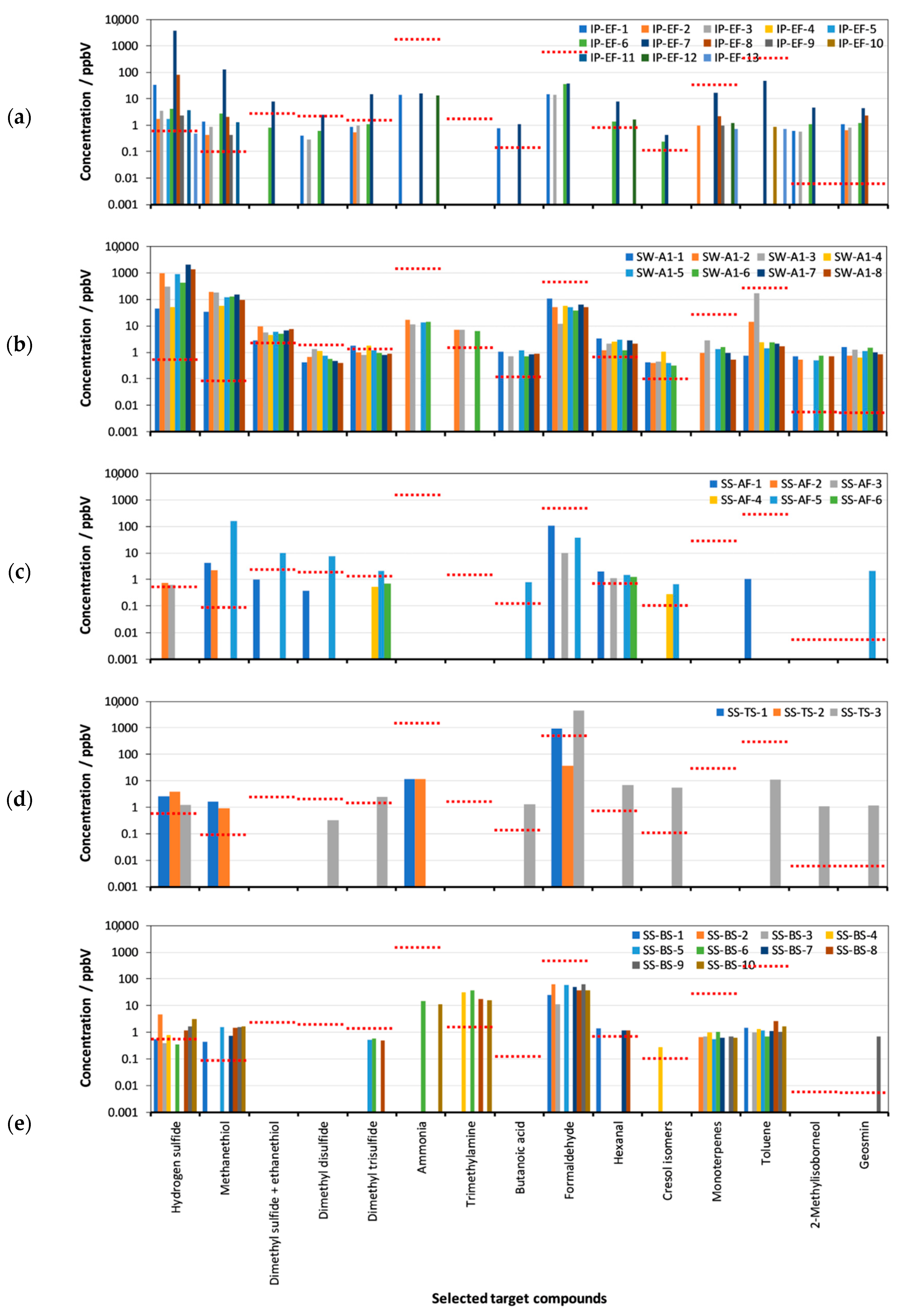
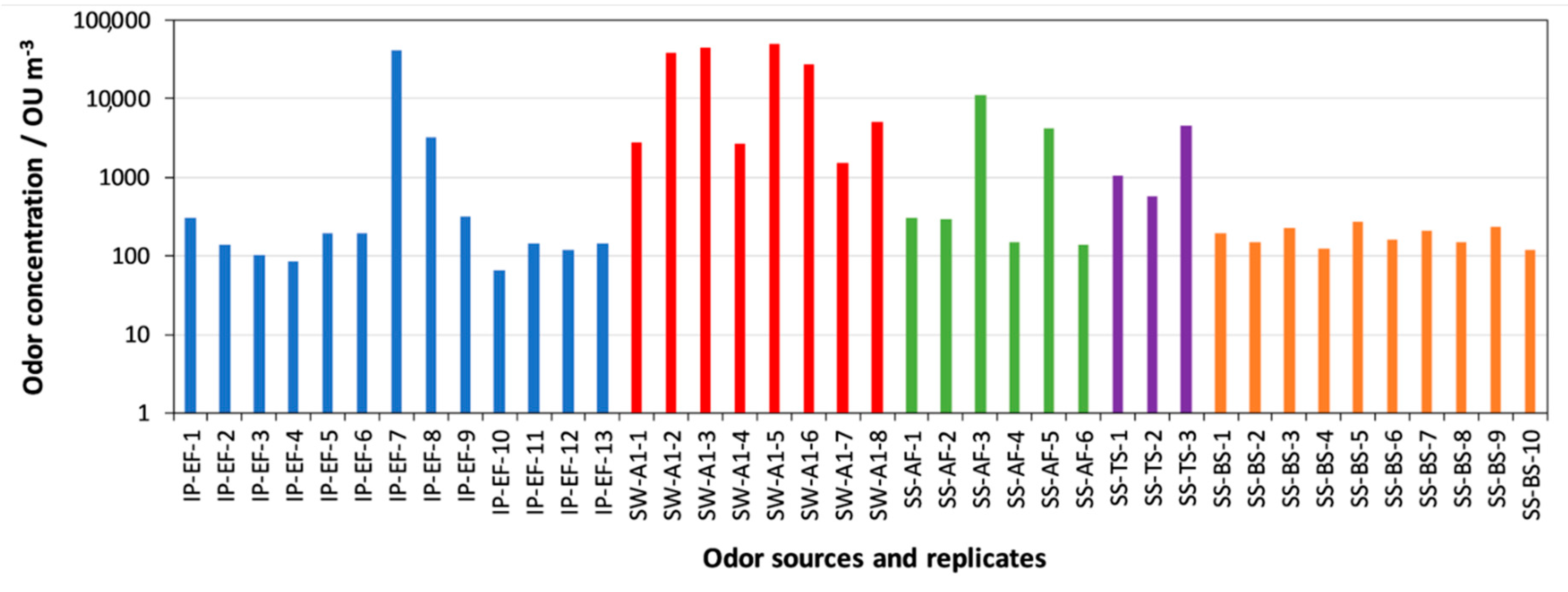
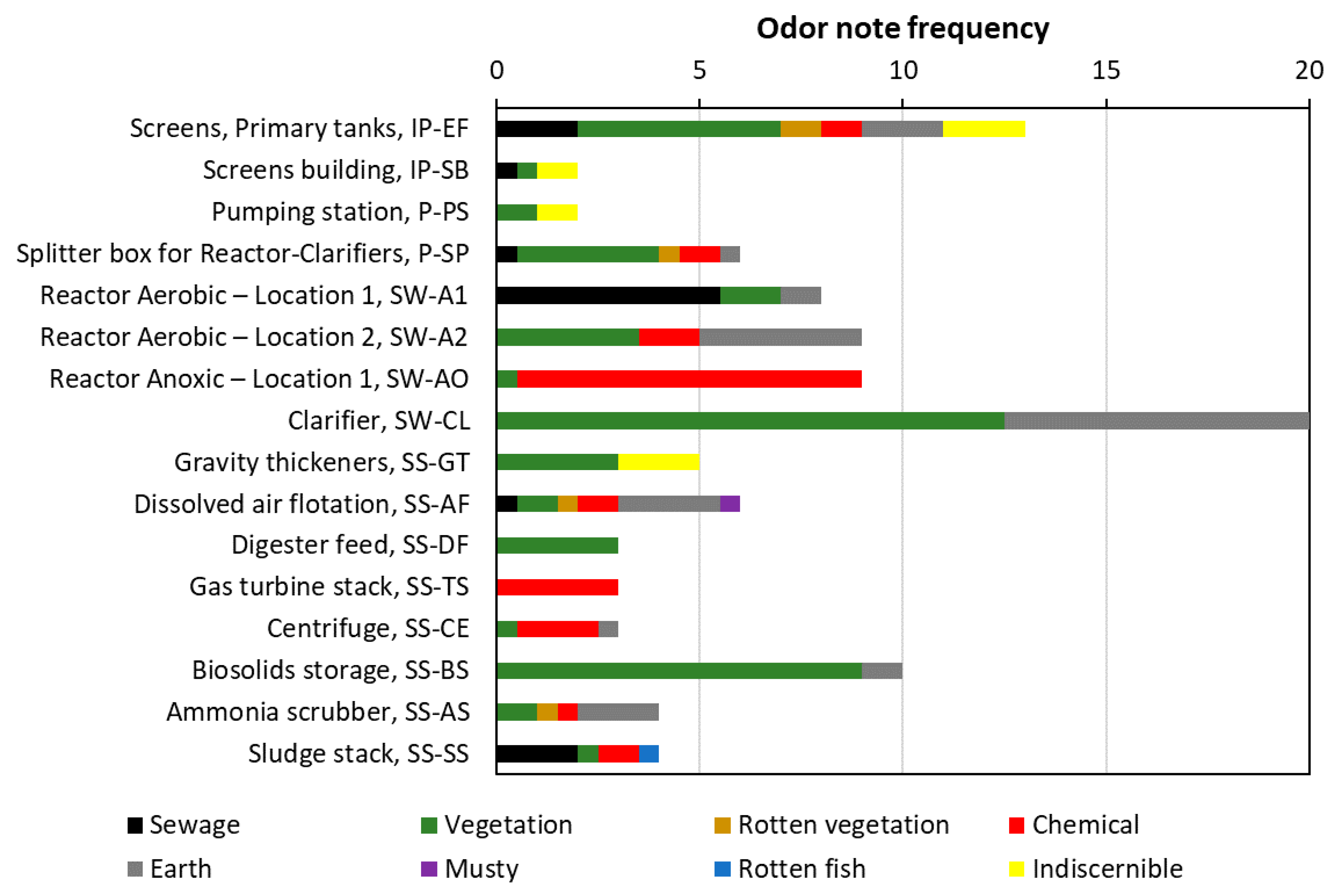
Figure 3 graphs represent a variety of odor sources throughout the treatment process and their associated sampling approaches. The chemical species variability within the same source was displayed along with the associated odor threshold value. Note that values less than the SIFT-MS LOQ are not shown. The ODT of each compound was indicated using a dotted red line. The sensory data (Figure 4) corresponding to these odor sources (Figure 3) showed similar individual sample variability for many reasons discussed later. There was variability in these representative sources of odor notes (Figure 5). In Figure 5, a frequency of unity is assigned where a single note is recorded, while each note was assigned a frequency of one-half when two are recorded.

To facilitate comparison of instrumental concentration data with sensory data, the concentrations were converted to OAVs using published odor detection thresholds. Only compounds with significant odor activities were further investigated. Hydrogen sulfide and methyl mercaptan were dominant in most odor sources. The odor compounds were grouped together in terms of primary odor categories defined by Fisher et al. [2].

Table 8. Primary odor categories for wastewater, their correlation with the sensory panel’s informal odor notes, and the most significant odor-active compounds detected using SIFT-MS.

Primary Odor Category 1	Sensory Panel Lexicon Oodor Note 2	Compounds Included (* = Not Included in Total)
Earthy/musty	Earth, musty	Not considered 3
Fecal/manure	Sewage	Cresol isomers
Fishy/ammonia	Rotten fish	Ammonia, isopropylamine, trimethylamine
Natural/fresh	Vegetation	Pentanal isomers, hexanal, monoterpenes
Rancid/putrid	-	Butyric acid, butanal isomers
Solvent	Chemical	Formaldehyde, acetaldehyde, propanal, ethanol, toluene, C4-alkylbenzenes
Sulfur	Sewage, rotten vegetation	*Hydrogen sulfide, *methyl mercaptan, dimethyl sulfide + ethanethiol, dimethyl disulfide, dimethyl trisulfide, diethyl disulfide, propyl mercaptans (total), butyl mercaptans (total)

¹ From Reference [2]. ² From sensory panel results (see Methods section). ³ For reasons described in the text, compounds in this class are not detectable in wastewater using SIFT-MS.

summarizes the key odorants, the primary odor category to which they have been assigned, and their correlation to the odor wheel of Fisher et al. [2] with the odor notes from the sensory analysis conducted here. Note that the characteristic “earthy/musty” odor notes for wastewater may be attributed to the presence of geosmin and 2-methylisoborneol [35]. Due to their very low ODTs (lower than the instrumental LOQ) and the complexity of the volatile emissions from the wastewater matrix, these compounds could not be detected and quantified reliably using SIFT-MS, so are omitted from the analysis. Fisher et al. [2] were unable to detect these compounds with GC/MS due to the very low ODTs. These compounds may still influence the odor character and olfactometry concentration as the method is designed to report the minimum odor threshold concentration.

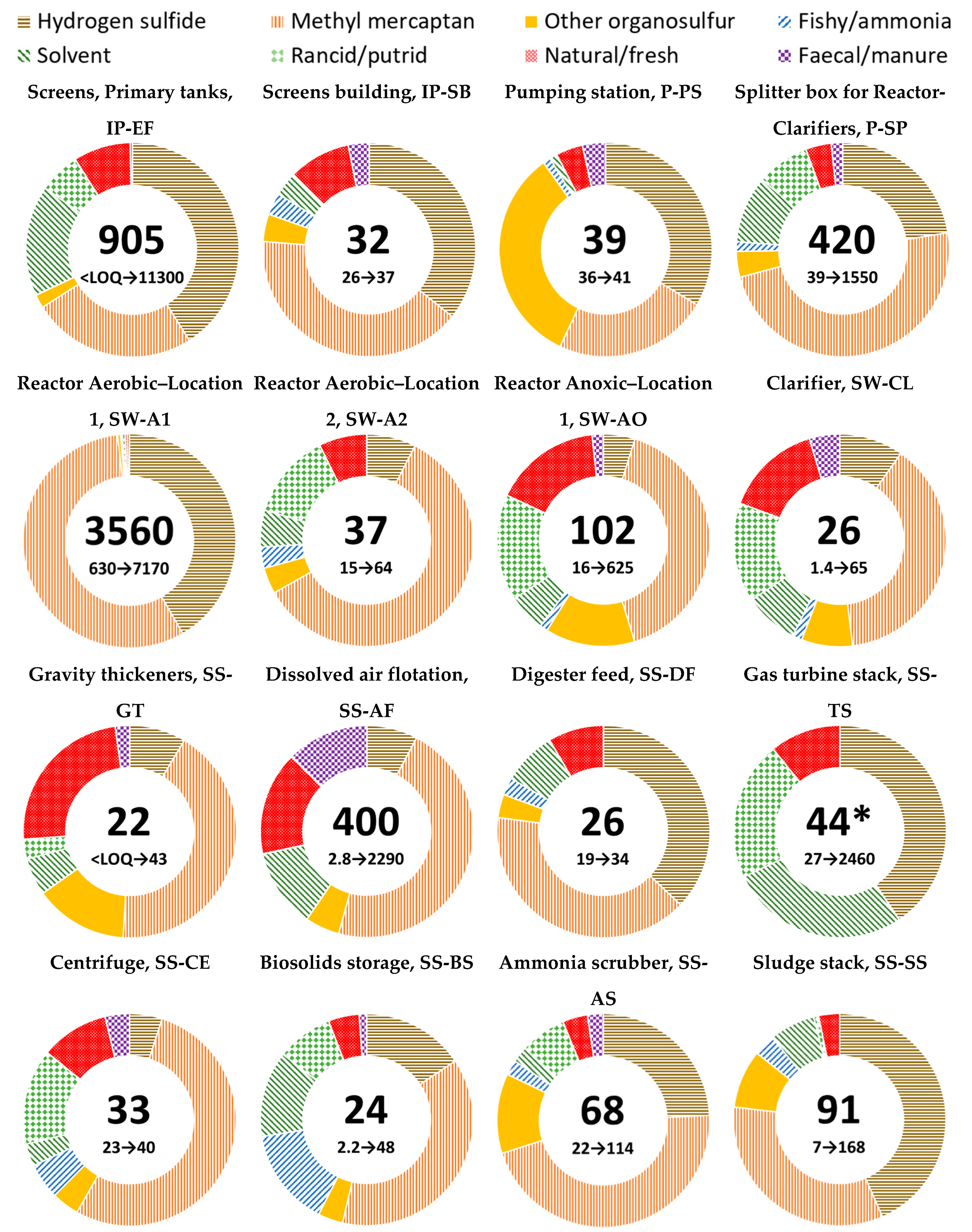
Figure 6 shows the odor composition determined using SIFT-MS for each odor source, together with the total OAV obtained from the sum of the key odorants. Mean concentrations of different source samples were used (a zero value was used when the SIFT-MS measurement was <LOQ) as a representation of that source. This was performed due to discreet sample variability at the same source. The range of total OAVs for the source is noted under the mean to indicate spread. In contrast to the concentration-based figures, the sum of hydrogen sulfide and methyl mercaptan OAVs dominated the odor for many sources.

Interestingly, the hydrogen sulfide ratio reduces during the wastewater treatment process. Hydrogen sulfide is high in the screens and primary sewage samples. The liquid process then moves through an 8-zone alternating anoxic/aerobic step-feed reactor process to the clarifier. A reduction in the ratio of hydrogen sulfide can be seen along this secondary treatment process along with a reduction of the OAV.

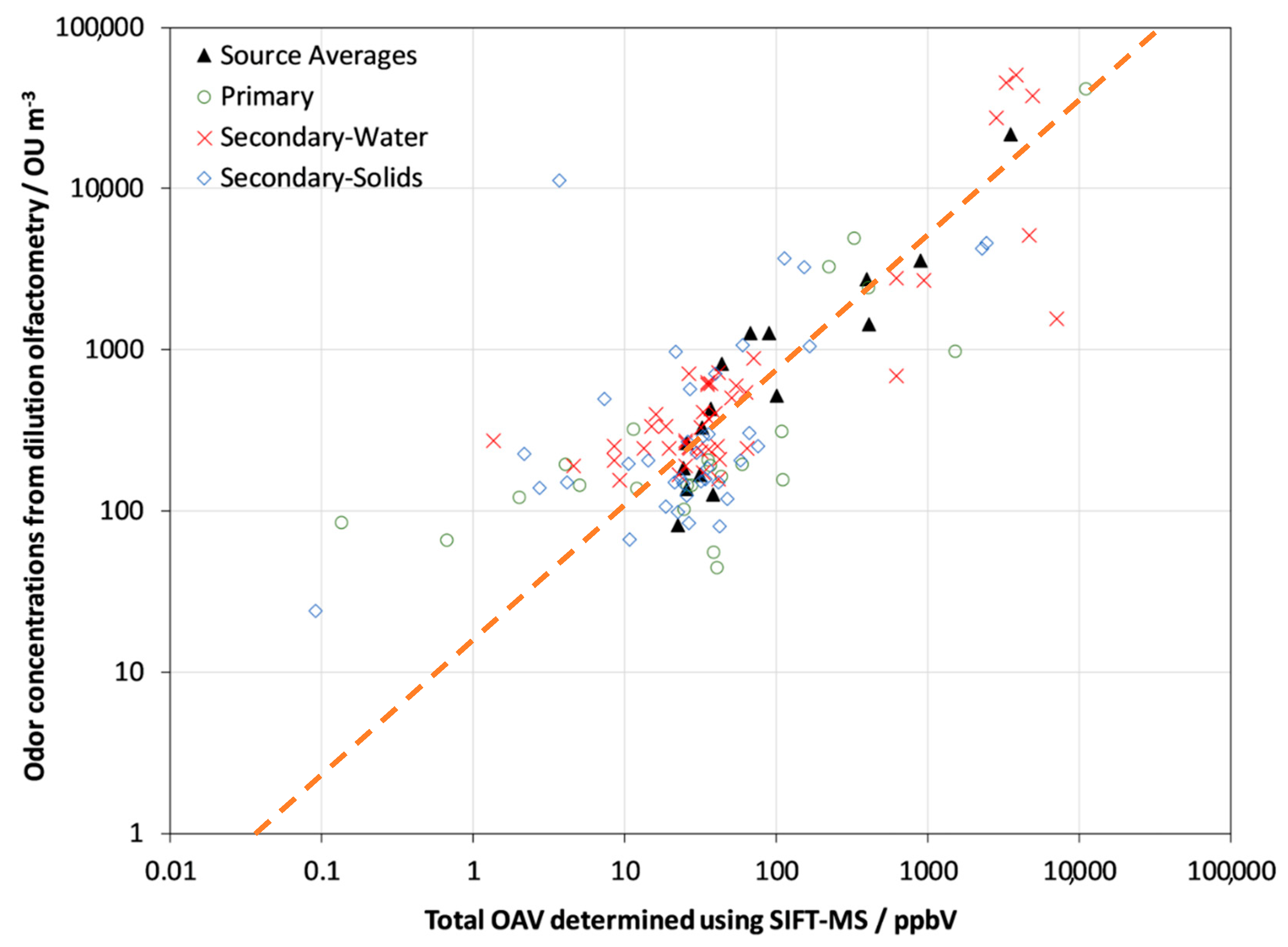
The total OAV for each sample was evaluated for its correlation with the odor concentration determined by the sensory panel. Figure 7 provides a comparison of the odor concentration determined by dilution olfactometry and the total odor activity determined using SIFT-MS. There is something of a trend as indicated by the dashed line.

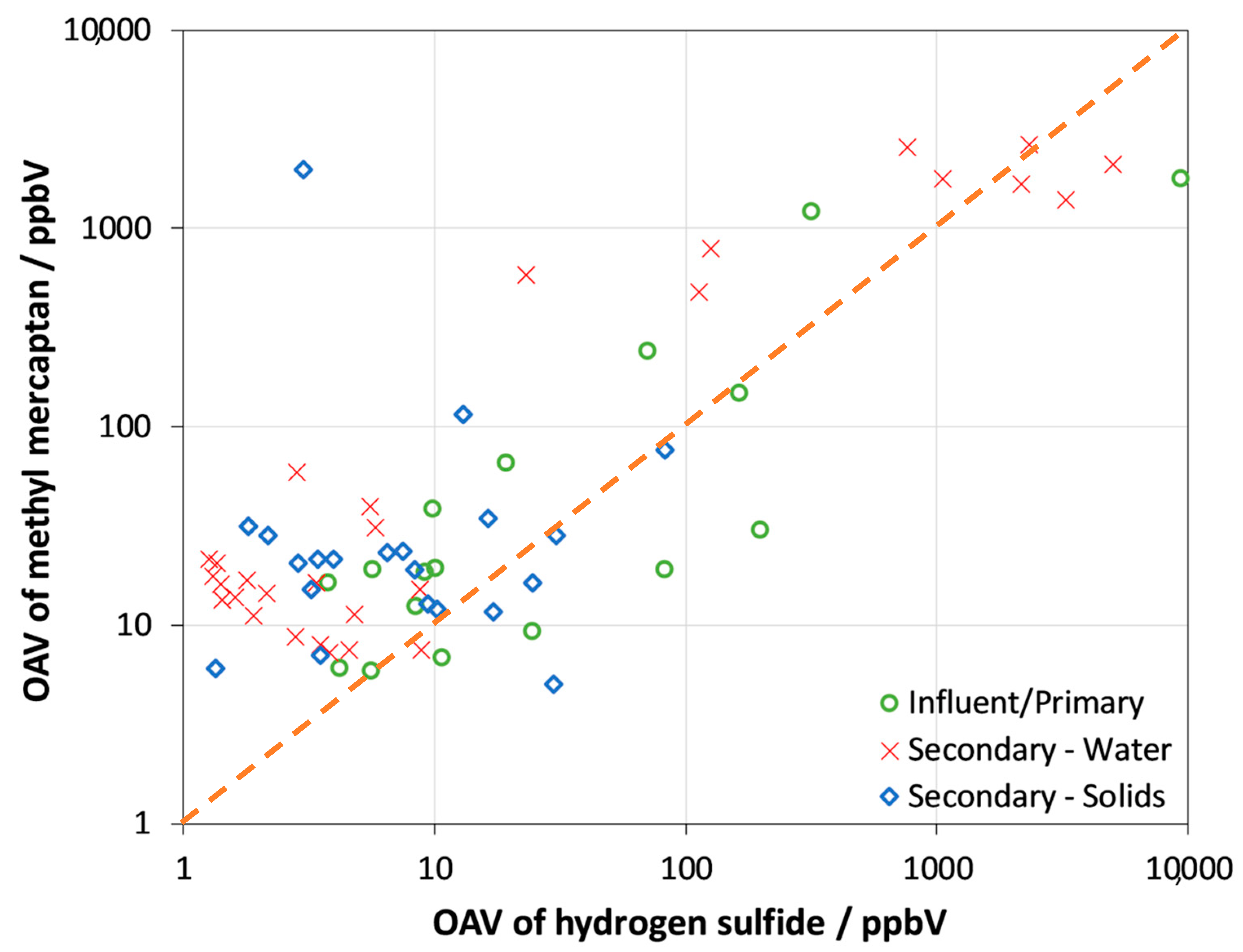
The results in Figure 6 suggest that methyl mercaptan may contribute more to the odor impact at different stages of the process than hydrogen sulfide, the most frequently measured odor indicator. Humans are more sensitive to methyl mercaptan than hydrogen sulfide based on their ODTs (Table 4). SIFT-MS quantifies hydrogen sulfide and methyl mercaptan with particularly high degrees of confidence, except when formaldehyde concentrations are elevated, and the sample is very moist (the gas turbine stack sample SS-TS-3 is the only occurrence in the present study). The results presented here suggest that hydrogen sulfide measurement does not serve as a surrogate measure of methyl mercaptan, as shown in Figure 8. This figure summarizes data for all samples in which both hydrogen sulfide and methyl mercaptan OAVs could be determined (i.e., they are greater than the instrumental LOQ).

4. Discussion

The purpose of this paper is to evaluate the potential of SIFT-MS for instrumental analysis of odorants in WWTPs through comparison with the literature and with sensory results obtained for the same samples. The aim of the ongoing two-yearly odor emissions study at the plant was to give an overview of odor emissions after odor mitigation systems have removed most of the odor from the raw source.

Each set of samples for each site were collected under potentially different operational and environmental conditions. These fluctuating conditions contribute to the variation seen at each site both in the olfactometry and SIFT-MS data. Another contributing factor to the observed variation is the location on the odor bed in which the samples were taken. Each location may have odor bed media of differing efficiency and compaction condition. Under dry conditions and without sufficient coverage of the sprinkler system (see

Table 9. Validated monthly rainfall approximately 2800 m west of the center of the plant.

Month	Rainfall in mm (10-Year Average 1)
October 2018	68.5 (105)
November 2018	85.5 (71)
December 2018	255 (84)
January 2019	40 (71)
February 2019	24 (68)
March 2019	34 (61)
April 2019	74.5 (78)

¹ 10-year averaged data for this site was sourced from www.metservice.com.

for an indication of rainfall conditions over the course of the study), media may dry out and short-circuits in the filter bed may form. If short-circuiting occurs, there may be regions of the media where odor species may not be sufficiently metabolized by the microorganisms in the media. This may allow regions to develop where higher olfactometry and odorant concentration may be observed compared to other parts of the odor bed. This is supported by the sampling approach. At each sampling round at each location, a randomized location was chosen to give the best representation of overall odor emissions. Other contributing factors included influent composition (ratio of stormwater, high industrial load, etc.), weather (humidity and air pressure), operating conditions (including natural flux of the microbial population, fan speeds, exact stage in the treatment process and maintenance schedule/cycle) and ambient temperature.

There are limitations to the detection of odors using olfactometry. As reported in Table 4, Table 5, Table 6 and Table 7, the odor detection threshold varies greatly between different chemical species. In addition, different odorants can react to the same odorant receptors with differing affinities, causing different responses at different ratios and concentrations within mixes of odorants [28]. In addition, there is variation between individuals regarding their response to the pleasantness of an odor [27]. If an individual finds an odor offensive, their personal odor detection threshold may be lower. There may be a different olfactory response at lower, diluted concentrations then would occur if smelling the undiluted, field sample. The complexities of odor detection and individual variation may also contribute to the variation seen in this study.

A study of hydrogen sulfide retention in Nalophan bags [36] suggested that Nalophan itself not only allowed the release of hydrogen sulfide over a 30-hr retention period, the Nalophan may have also absorbed some of the hydrogen sulfide. This was demonstrated by inserting additional Nalophan material into the bag to increase the surface area [36]. The bags used for olfactometry were long sausage shaped bags that contained between 30 to 40 L of gas. The Nalophan bags used for SIFT-MS analysis were made from the same roll of Nalophan and held around 5 L. Zip ties were used on either end to secure the bag shut and attach the Swagelok fittings. The gas in the SIFT-MS bags would have more surface area in contact with the Nalophan when compared to the olfactometry samples. Additionally, the samples for SIFT-MS analysis were shipped via courier to Hamilton and were not held in a temperature-controlled laboratory as the olfactometry samples were. Differing partial pressure within the bags due to varying rates of inflation may contribute to differing amounts of gas loss or gas mixture changes in composition. Another factor may be the formation of a gradient within the gas composition in the bag. Heavier gases such as hydrogen sulfide, may settle on the bottom of the gradient and more volatile compounds may rise to the top. This may affect the observed olfactometry and SIFT-MS results if mixing did not occur. Therefore, these differences may have resulted in a variance between the final gas composition for samples analyzed for olfactometry and SIFT-MS.

Below we discuss the applicability of both SIFT-MS and olfactometry in the different stages of the wastewater treatment process and look at ways the technologies can be used to assess odors within a plant. Individual sample IDs were referenced in this section, for which detailed data was provided in the Supplementary Materials submitted with this article.

4.1. Influent and Primary Treatment

Reduced sulfur compounds were expected to dominate the odor profile in the primary treatment phase [1]. Figure 6 shows a high ratio of hydrogen sulfide and methyl mercaptan in these primary treatment samples.

Screens for the primary tanks (IP-EF). Samples were acquired after biofiltration. Therefore, low concentrations of odorants were expected and were observed for most samples. However, sample IP-EF-7 displayed odor activities of 9350 and 1770 for hydrogen sulfide and methyl mercaptan, respectively. This outlier may be attributed to short-circuiting in the biofilter, where a path has developed through which air can migrate without sufficient interaction with odor-processing microbes. A section of the odor bed may have been dry and/or may require maintenance.

There was some agreement of SIFT-MS data with olfactometry results from the primary effluent samples. For the outlier, IP-EF-7, there is agreement of high OAV and strong sewage odor as characterized by the olfactory panel. Very low odor activity is observed for IP-EF-4, which is described as “indiscernible” by the panel. The SIFT-MS analysis did not detect chemical species described as displaying “vegetation” or “chemical” notes as described by the olfactory panel. The OAV data from SIFT-MS analysis for hydrogen sulfide and methyl mercaptan suggested that sewage odor compounds were the key odorants in many of the samples displaying characters described as “vegetation” or “chemical.” Concentrations of these compounds were recorded at lower levels compared to IP-EF-7. However, there is a possibility that the compounds responsible for the “vegetation” and “chemical” characteristics were not analyzed for by the SIFT-MS suite (see Table 4 for a list of included compounds). The characterization notes may be attributed to the bark on the top of the biofilter. Additional analysis of volatile organic compounds emitted from the bark, such as alpha- and beta-pinene, may give insight into the contribution of the media to the odor characterization when the sewage-related compounds have been metabolized below their ODT.

Screens building (IP-SB). The two ambient samples analyzed were taken at the door of the screens building using a grab approach at nose height. OAVs of reduced sulfur compounds were low for an influent odor source consistent between the two sampling episodes. This may be attributed to the samples being ambient gas and not directly from an odor source. The “very light sewage/vegetation” attribute for IP-SB-2 correlates with the SIFT-MS analysis. Whereas the “indiscernible” character attributed to IP-SB-1 by the panel does not. A sewage odor signature was predicted from the SIFT-MS analysis to be the dominant odor character of this sample. As this was an ambient sample, odors from additional compounds to those analyzed by SIFT-MS may have been present. Ambient samples may also be more influenced by wind speed and direction and other meteorological parameters than samples taken from biofilters and liquid interfaces. Interfering odors from other parts of the site may be present that were not detected by the chosen SIFT-MS suite.

Pumping station (P-PS). Only two samples were acquired from these sources and they follow biofiltration. P-PS-1 has no hydrogen sulfide detected above instrument LOQ or odor threshold, while methyl mercaptan is detected in both. The “indiscernible” and “very light vegetation” characters provided by the sensory panel for samples P-PS-1 and P-PS-2 respectively, were not expected from the SIFT-MS analysis profiles. The SIFT-MS data suggested a “sewage” or “rotting vegetation” character may seem more likely (some “vegetation” character may be imparted by low levels of C₅ and C₆ aldehydes, however, these are lower in odor activity than the sewage contributors). Organic compounds relating to the biofilter medium may have dominated the odor character and may not have been analyzed by the wastewater-focused SIFT-MS suite used here.

Splitter box for reactor-clarifiers (P-SP). The dominate odor-active volatiles in these post-biofilter samples are again hydrogen sulfide and methyl mercaptan, with smaller contributions from a variety of C₄-C₆ aldehydes. Monoterpenes and toluene occur above the odor threshold for P-SP-4 and P-SP-3, respectively. The aldehydes detected may contribute to the “(very) light vegetation” notes frequently attributed by the sensory panel. However, the absence of “sewage” characters described by the odor panel for most of these samples was unexpected. The OAVs of both hydrogen sulfide and methyl mercaptan were expected to contribute to a sewage character. For P-SP-6, in particular, a “moderate sewage” odor character might have been expected based on the SIFT-MS results and calculated OAV. Again, organic compounds may have been present that were not analyzed via SIFT-MS. These may have contributed to the experienced odor characters in the laboratory.

4.2. Secondary Water Treatment: Reactors/Clarifiers

All samples from this phase were acquired using flotation sampling on the exposed liquid surface; that is, there was no biofilter to remove odorants prior to sampling. Hence, the odor measured was consistently higher in the first aerobic location (SW-A1) of the reactor/clarifier when compared to other locations further along the treatment process. SIFT-MS results reported a dominance of reduced sulfur compounds and a higher OAV in the first aerobic zone when comparing results to the aerobic zone later in the treatment process. The reduction in odor is expected as the nutrients are reduced. Little has been documented regarding the changes to odor concentration and odorant composition throughout the reactor/clarifier process. Most papers currently describe odorants from the WWTP in its entirety (e.g., [1], [2] and [37]) or with a focus on biosolids (e.g., [2]). In the second location of aerobic processing and in the final stage of anoxic processing, the total odor activity was reduced and approximately 40% of the odor measured using SIFT-MS was attributed to non-sulfur species. The reduction in measured concentrations of the volatile sulfur compounds (Table 6) concurs with this. This may indicate that most of the organic matter is removed in the first stages of the process releasing large amounts of sulfur species [1,38]. However, the reactor is zoned in a step feed process where influent is added in varying amounts to each of the anoxic zones. The first anoxic zone does contain the highest amount of primary treated influent when compared to anoxic zones 5 and 7 later in the process. To better understand the gases produced, a SIFT-MS study in conjunction with metagenomic and/or proteomic analysis of the biomass and detailed chemical analysis of the influent may be useful in determining which microbial species are producing the gases present from what substrates.

Reactor aerobic—location 1 (SW-A1). Hydrogen sulfide and methyl mercaptan dominate the odor activity of this treatment. The SIFT-MS data agree well with the odor panel, except for samples SW-A1-1 and SW-A1-4. For these samples, both hydrogen sulfide and methyl mercaptan OAVs were recorded in the 100s range, indicating a moderate to strong sewage odor would be expected. Whereas the panel attributed a “moderate earth/vegetation” note to SW-A1-1, and a “light vegetation” note to SW-A1-4. The absence of sewage notes in the descriptors provided by the sensory panel may be due to the presence of additional organic odorants.

Reactor aerobic—location 2 (SW-A2). As the wastewater at location 2 has undergone further processing compared to the wastewater at location 1, one would generally expect lower concentrations of odor and odorant species. This was indeed the case for SW-A2-2 to SW-A2-9. Of the compounds measured using SIFT-MS, methyl mercaptan was the dominant odorant in this location. SW-A2-1 was an outlier, with high OAVs for both hydrogen sulfide and methyl mercaptan (3260 and 1380 ppbV, respectively). Samples are collected at random and are not collected with the daily peak loads in mind. During the course of a day, loads on the reactors can differ. As the samples were collected over the course of four months, the study is designed to capture a range of seasonal and daily variation. In zone 8, increased airflow and higher dissolved oxygen set points are used to remove any remaining ammonia. Higher dissolved oxygen in this location (relative to zone 2) may be increasing the activity of a subset of the aerobic bacteria capable of generating methyl mercaptan from waste [39]. Operational processes were not monitored or included for the purpose of this study. Therefore, there is no recorded information to compare the sampling data to operational decisions. There may also be variation in the composition of the raw effluent or the microbial communities present in the reactor/clarifier sampled over the course of the sampling period.

SIFT-MS data did not support the most frequent “vegetation” character described by the panel. The SIFT-MS analysis predicted that all samples should still have a light to moderate “sewage” note. The “earth” character was not reliably predicted using SIFT-MS in this study. Additional organic species may be present that created this odor character. More research regarding the understanding of the olfactory response (from odor receptors to olfactory bulb mapping of an odor) may be required to assist in the generation of a more refined odor prediction method.

Reactor anoxic—location 1 (SW-AO). OAVs were low for the late-stage anoxic zone investigated in this study as would be expected for samples taken from the end of this treatment process where primary treated influent is added at a reduced rate than anoxic zone 1. Methyl mercaptan remained the most prevalent odorant contributor in many samples. However, methyl mercaptan was below the instrumental LOQ in several samples. It potentially may have been still above the human ODT. Other significant odorants detected were dimethyl trisulfide and C₂-C₆ aldehydes. However, overall chemical composition was highly variable from sample to sample in this location. Smaller aldehydes (C₁-C₃) may have contributed to a chemical odor characteristic [4], in agreement with the sensory data. However, Gostelow et al. [1] describe butanal as having a “rancid/sweaty” note. For SW-AO-1 and -2 these small aldehydes have OAVs similar to those of methyl mercaptan. A better understanding of the chemical sensory signal in the olfactory system is required before we can make clearer assumptions regarding the perception of these odorants in a complex gas mix.

Clarifier (SW-CL). In general, the odor-active volatiles from this phase were similar to those of the anoxic location (SW-AO) above. This is expected as the clarifier is an anoxic environment with influent from reactor zone 8 with the purpose of settling out solids (including biomass). There was one outlier in the 20 samples analyzed (SW-CL-1). In this sample, hydrogen sulfide and methyl mercaptan OAVs were at 23 and 580, respectively. This may be due to many variable factors operationally or the chemical composition of the primary effluent. However, in spite of the presence of hydrogen sulfide and methyl mercaptan, the sensory analysis does not seem to detect the complete odor mix as a “sewage” odor. The character was described as “moderate earth”. For the other samples, the comments for SW-AO apply.

4.3. Secondary Solids Treatment

Total OAVs were lower throughout these processes. The highest values obtained were from samples taken from the DAF. Overall the reduced sulfur compounds were significantly lower in secondary solids treatment than in primary and secondary water treatment.

Ammonia was measured marginally above the human odor threshold in a very small number of samples. Trimethylamine was detected occasionally at low ppbV throughout the treatment process. This chemical was most prevalent from biosolids stabilization onwards (that is, detected in samples taken from the biosolids storage biofilters, and the sludge stacks). Only in one of the sludge stack samples was a fishy note detected by the odor panel. The SIFT-MS odor data agrees well, with chemical odorants generating a fishy character being reported as a small fraction of the odorous chemical species analyzed.

Vegetation characters were consistently described as the dominant odor character in the sensory analysis. SIFT-MS detected several aldehydes in these samples, although only marginally above the currently determined odor threshold. Due to high olfactory system genetic variability between people, each olfactory panel may essentially have their own unique odor threshold for different chemicals where their associated receptors may have high genetic variation within the general population. Panel members are screened for suitable odorant sensitivity using one chemical species only (n-butanol). There may be other chemical species that some of the participants may be very more sensitive to due to genetic variation in their olfactory receptors. There may also be a compounding effects of multiple odorous species in the mixture on a single receptor.

Gravity thickeners (SS-GT). OAVs were low in samples taken from the biofilters in this phase. However, most samples reported measurable hydrogen sulfide and methyl mercaptan. For some samples, low molecular weight aldehydes have small, measurable odor activities. Overall a light “sewage” note would be expected, but sensory analysis reported “vegetation” or “indiscernible”. SIFT-MS agrees with the latter for SS-GT-4, but not for the other samples. As discussed previously, some characters may be influenced by emissions from the biofilter materials and not analyzed by SIFT-MS in this study. These compounds may also be below the limit of detection. A study of baseline biofilter odor characteristics may assist in understanding the character described by the panel.

Dissolved air flotation (SS-AF). This was the only phase in secondary solids processing where flotation sampling was carried out. For all but SS-AF-5 (with methyl mercaptan having an OAV of 2210), odor activities were low considering that there was no biofiltration. Hydrogen sulfide was always less than an OAV of 2 in these samples, while methyl mercaptan was only detected in the above-mentioned sample, plus SS-AF-1, and SS-AF-2.

SIFT-MS analysis of sample SS-AF-2 (“light sewage”) agrees well with sensory analysis, while SS-AF-5 partially agrees. The “rotten vegetation” note may be attributed to methyl mercaptan in the absence of hydrogen sulfide. Further studies of known odorant mixes may be required to determine how different odorant mixes effect odorant perception.

Digester feed (SS-DF). SIFT-MS OAV profiles predicted a “light sewage” note in contrast to the “(very) light vegetation” note as characterized by the sensory panel. As described in previous sections, the odorous gas from this part of the plant was pre-treated in an odor bed containing 30% aged bark (see Table 1 for more details). The described “light vegetation” odor may be attributed to the microbial communities in the odor bed and the emissions from the bark. There may be compounds present that were not analyzed by SIFT-MS and hence not included in the odor profile generated.

Gas turbine stack (SS-TS). Of the three stack samples taken from the turbines, only two can be usefully discussed or compared. SIFT-MS and sensory results agree well for the first two stack samples–the “chemical” note may be attributed to the presence of low molecular weight aldehydes.

The outlying sample, SS-TS-3, may have been taken under different feed gas composition and/or stack operating conditions [40], which may have resulted in incomplete combustion as indicated by the elevated aldehyde readings. Increased alcohol concentrations in biogas can cause increased aldehyde emissions from combustion. No samples were taken of the pre-combusted biogas to provide any more insight [41].

Formaldehyde formed through combustion precludes reliable analysis of methyl mercaptan in the moist stack conditions. This is due to the water adduct of protonated formaldehyde being isobaric with protonated methyl mercaptan. In samples with high aldehyde content, only hydrogen sulfide can be measured meaningfully using SIFT-MS. Other reduced sulfur compounds that were likely present were not analyzed due to the interference of the aldehydes. Therefore, without reliable analysis of sulfur compound composition, a meaningful comparison to olfactometry could not be provided in this sample.

Centrifuge (SS-CE). Methyl mercaptan and some small aldehydes were present in the odor activity profile generated by the SIFT-MS data for the odor bed treated centrifuge plant gas. The presence of small aldehydes concurs with the “chemical” notes as detected by the sensory panel for two of the samples. The third sample was described by the panel as containing a “vegetation” character. The aged bark in the biofilter may have contributed to this observed odor character and may have been more dominant than the organic notes that would be expected to display “sewerage” characteristics.

Biosolids storage (SS-BS). Odor activity was low in these samples. Measured odorants were highly variable from sample-to-sample. This may be attributed to the ambient samples being collected near the door of the biosolids storage building. The wind speed and direction may contribute to the type of odorants collected as well as the disturbance of the biosolids products at the time of sampling due to mechanical movement of the biosolid material (i.e., loading lime-treated biosolid material into trucks). Much of the odorant gas may be removed by the ventilation system within the biosolids shed. The odorant gas is blown out the stacks at the rear of the building. Samples collected within the building at times of high mechanical disturbance of the biosolids may have produced a much higher result.

Dominant volatiles on occasion include hydrogen sulfide, methyl mercaptan, trimethylamine, and the low molecular weight aldehydes. Trimethylamine was expected to be present in biosolid gas due to biosolids stabilization with lime [6].

“Vegetation” and “earth” were described as the odor characters present from the olfactometry panel. “Vegetation” notes may be attributable partly to the presence of aldehydes. From the SIFT-MS analysis, a “light sewage” character would be expected due to the sulfur and rancid/putrid compounds present. In addition, the ammonia scrubber odors pass through a biofilter prior to collection. The biofilter bed was comprised of 26% Compost / Pumice. This compost component may have contributed to the “vegetation” and “earth” odor notes described by the olfactory panel.

Ammonia scrubber (SS-AS). From the ammonia scrubbers, only one sample reported levels of ammonia above the detection threshold. However, hydrogen sulfide and methyl mercaptan were also detected along with some of the smaller aldehydes. “Earth” and “vegetation” odor notes were described by the olfactometry panel. The SIFT-MS data analysis expected to see a “sewage” note as being more dominant. The scoria and compost/pumice-based odor bed may have contributed to the earthy odor characters described by the olfactometry panel.

Sludge stack (SS-SS). SIFT-MS data obtained from four samples suggested variability of the absolute and relative abundances of hydrogen sulfide and methyl mercaptan. In addition, one sample reported the highest trimethylamine measured in this study (SS-SS-2). Other reduced sulfur compounds and aldehydes were present around or slightly above the ODT.

Variance was also seen when olfactometry samples collected at different times were compared to each other. A “sewage” note was identified for SS-SS-2 and SS-SS-4. From the odor activities reported using SIFT-MS, it was predicted that the intensity for SS-SS-2 would be described as moderate as per the description for SS-SS-4. This is another example outlining the subjective nature of the olfactometry method and the complexity of odor analysis. It is difficult to assign one single odor character and choose a level of intensity that conforms to a repeatable standard. Odor fatigue can occur when large sets of samples are presented to the odor panel. The intensity descriptions may be affected by the strength and composition of the preceding samples as odors are described and characterized as a form of reference only. Only one character can be chosen by the panel.

A “light rotten fish/chemical” character was expected from the SIFT-MS results of sample SS-SS-2, as it reported elevated trimethylamine. A “light rotten fish/chemical” odor was characterized by the odor panel in sample SS-SS-3. The SIFT-MS analysis reported hydrogen sulfide levels only slightly above the ODT and several aldehydes at the ODT (which could give the “chemical note”). SIFT-MS did not report odorants associated with “chemical” or “vegetation” characters in the SS-SS-1 sample as per the olfactometry characters described. In this sample, hydrogen sulfide and methyl mercaptan were reported well above their ODTs (OAVs of 30 and 5.0 ppbV, respectively).

There are many variables that may have affected the gas composition both in the olfactometry lab and the samples provided for SIFT-MS. Samples for SIFT-MS were sent via courier to Hamilton. This drive was not temperature controlled like the laboratory conditions for the olfactometry samples. The resulting gas composition in the SIFT-MS samples may have changed during this trip. In addition, the surface area of Nalophan to gas sample was increased with the smaller SIFT-MS samples. As per the experiments of Eusebio et al. [36], the increased surface area may have contributed to the adsorption of hydrogen sulfide and other gases when compared to the olfactometry sample gas composition. The increase in gas volume of the samples used for olfactometry, may have assisted in keeping the chemical composition more stable. A SIFT-MS analysis of the same samples in the same location as the olfactometry panel would be more ideal when comparing both methods to reduce these variables.

There may have been compounds not analyzed via SIFT-MS that were contributing to the odor profiles and characters described by the panel. Increasing the odorous gases present in the SIFT-MS library and optimizing the analysis to include as many of these compounds as possible would be the best way to capture more compounds and determine their effect on the overall described odor.

4.4. General Comments on Odor Analysis Using SIFT-MS

There are limitations to this comparison as the chemical species related to earthy odor notes that feature in many low odor concentration samples are not detected using SIFT-MS. In addition, olfactometry gives you a threshold limit of detection of an odor and so complex samples with compounds that have lower ODT’s can produce higher olfactometry results compared to the associated OAVs [5].

As demonstrated above, the low LOQs and selectivity of SIFT-MS make it a generally applicable tool for odor analysis at WWTPs, but it is not a single solution.

SIFT-MS can be utilized to target a wide range of odorants, as shown in Table 4, but the complex wastewater matrix does create some issues. It reliably quantifies the most notable wastewater odorants that give the “sulfur” or “sewage” odor—hydrogen sulfide and methyl mercaptan. This study demonstrated that the use of hydrogen sulfide in isolation as an indicator of odor, is not reliable. The levels of hydrogen sulfide and the more pungent sulfur odorant, methyl mercaptan, are variable amongst sources (Figure 8). Additionally, SIFT-MS can be utilized to target compounds that contribute to the “natural/fresh” or “vegetation” note, the “solvent” or “chemical” note, and the “fishy/ammonia” or “rotten fish” note. However, for these the dominant note predicted from the odor wheels (Figure 6) does not always compare well with those given informally by the sensory panel. Since most of the relevant odorants are detected by SIFT-MS at levels below the published ODTs, SIFT-MS is generally considered more reliable. However, one pungent WWTP odorant with a “chemical” note is not detected selectively: 2,3-butanedione.

For the “earthy/musty” note, SIFT-MS currently does not have sufficient selectivity to detect the extremely pungent odorants geosmin and 2-methylisoborneol of this odor character [2]. The sensory panel did not use “rancid/putrid” and “fecal/manure” descriptors at all, probably due to the common language usage that was informally employed, despite them featuring in published odor wheels [2,4,37]. Due to the complex matrix, SIFT-MS does not analyze several pungent compounds in these odor notes with sufficient selectivity; in particular, pentanoic acid, indole and skatole. For these compounds, plus geosmin and 2-methylisoborneol, the low ODTs compared to more generic odorants found in wastewater means that they are very susceptible to over-reporting when converted to OAVs.

Can SIFT-MS identify process abnormalities? On a sample-by-sample basis, SIFT-MS appears helpful for rapidly and reliably detecting many of the gases formed during biological processes on site. Monitoring changes in the gas composition could assist operational staff better understand changes to the biological and chemical reactions taking place in the reactors. Examples shown here include incomplete combustion in a gas turbine stack (SS-TS-3), short-circuiting in bio- or earth filters (IP-EF-7) where hydrogen sulfide is not an appropriate indicator, and elevated odor concentrations being emitted from a later stage aerobic location in a reactor-clarifier (SW-A2-1). Direct analysis on site using a mobile SIFT-MS instrument and a biofilter hood may assist in pinpointing of short circuits in bio- and earth filters, for example, and identify areas where maintenance of odor beds is required especially where hydrogen sulfide is not an appropriate indicator.

Can SIFT-MS differentiate odor sources based on chemical analysis at the plant boundary? The large variations observed in this study for the more odorous process phases suggest that it would be very difficult to identify problems in individual processes. Preliminary evaluation of the data using multivariate statistical methods suggest that it is not feasible. However, continuous monitoring using SIFT-MS would provide immediate, sensitive indication that there is an emerging issue at the WWTP and provide a more comprehensive “odor print” than just hydrogen sulfide. In addition, the species determined by SIFT-MS in conjunction with metagenomic analysis can give insight into the microbial population within the reactors and more specific metabolic information surrounding the process. Changes to influent composition could be detected by SIFT-MS odor analysis such as a rise in odors associated with decomposing fats or animal tissues or biologically detrimental chemicals that could be toxic to activated sludge biomass.

Can SIFT-MS be used to predict the odor concentrations determined using dilution olfactometry (i.e., OU m⁻³)? Initial attempts to answer this question utilized principal component regression [42] because this is a multivariate calibration problem: i.e., prediction of odor unit based on the odorants detected by SIFT-MS. Prediction is poor no matter what approach is taken (e.g., using individual odorant OAVs or grouping those odorants of similar odor note). There are likely two reasons for this. First, SIFT-MS is not analyzing all odorants effectively, with the absence of reliable “earthy/musty” note likely being the most significant. A sample of “moderate earth” character (SS-AF-3) illustrates this situation, with an odor concentration of 11,205 OU m⁻³ but a total odor activity of only 4 ppbV calculated from the dominant odorants analyzed with SIFT-MS. Instead a simple correlation of total odor activity value for the dominant, reliably analyzed odorants with odor concentration was attempted (Figure 7). There is a trend indicating general agreement between olfactometry and the total odor activity, but since SIFT-MS is not quantifying compounds reliably that have “earthy/musty” notes, there are also significant outliers, such as the one mentioned above.

Braithwaite [5] questions the reliability of dynamic dilution olfactometry, despite it forming the basis of numerous standard methods globally (e.g., AS/NZS 4323.3:2001, BS EN 13725). Braithwaite [5] summarizes the situation:

“As an odor mixture is diluted, the odor notes and hedonic tones change and eventually, after sufficient dilution, the concentration of the final detectable odorant drops below its odor detection threshold, so the diluted sample becomes ’odorless‘. The amount of dilution required to reach this point is considered an indicator of the odor intensity of the initial, undiluted sample, which is problematic because the final detectable odorant may not be indicative of the odorant that dominated the odor of the undiluted sample (nor the dominant odorant in the partially diluted sample at the fenceline). Relying on dilution quantities to indicate the intensity of the total odor is crude at best and misleading at worst.”

Can SIFT-MS predict the odor note? The results presented here show agreement for less than half of the samples tested. Agreement is primarily in terms of the “sewage”, “chemical” and “vegetation” notes provided informally by the sensory panel. However, the absence of “sewage” notes from the sensory panel in many samples where SIFT-MS detects hydrogen sulfide and methyl mercaptan as dominant odor-active volatiles suggests that the informal approach to odor note determination is a crude description of the odor. The SIFT-MS analytical suites were chosen based upon expected wastewater odorants and may not have analysed every odorous compound associated with bark and soil in the biofilters. Hence no firm conclusions can be made at present. Another point to consider is the change in odors present in the sample from time of sampling to analysis. While samples are analyzed within the 30-h window, their chemical composition can likely be altered over this period as different gases interact with each other and other gases are absorbed into the Nalophan. A field SIFT-MS instrument would eliminate this issue.

Can SIFT-MS predict odor intensity and hedonic tone? Odor intensities listed in Table 5, Table 6 and Table 7 and the supplementary data are from informal sensory measurements based upon standard odor detection threshold methods. The panel did not evaluate hedonic tones. The data, therefore, do not facilitate evaluation of intensity and hedonic tone versus SIFT-MS measurements. This will need to be evaluated in another study.

5. Conclusions

The wastewater matrix is challenging due to its complexity and variability. SIFT-MS selectively detects and quantifies many, but not all, of the key odorants. The SIFT-MS data correlate well with the literature reviewing the important odorants in WWTP process, except for the “earthy/musty” odor, which cannot be selectively analyzed currently. Characteristic “sulfur” (or “sewage”) odor is readily and sensitively detected, even in samples where informal sensory analysis misses it. SIFT-MS unequivocally demonstrates that hydrogen sulfide is not a reliable sole marker for WWTP odor.

Total OAVs determined using SIFT-MS correlate loosely with the odor concentration determined by sensory panel using dynamic dilution olfactometry. Samples that do not correlate well are attributed to the inability of SIFT-MS to detect “earthy/musty” notes effectively in the WWTP matrix and to the known limitations with this sensory method.

Compared with other analytical techniques used for odor analysis, the results obtained with SIFT-MS compatible with the number of compounds that can be detected at below or approaching human ODTs. However, SIFT-MS does not provide a comprehensive solution for WWTP odor analysis. Nevertheless, because fenceline odors are more frequently attributed to the “sulfur” or “sewage” note, than any other note, there are applications for SIFT-MS in WWTPs. These include continuous monitoring at the fenceline to provide rapid indication of developing odor issues so that they can be resolved before they become a major issue with neighbors, and the possibility of mobile instrument operation on-site to identify the source of an odor issue.

Braithwaite [5] has recently recommended SIFT-MS as part of a multi-methodology approach for odor research, in which SIFT-MS is combined with GC-Sensory (GC-MS/O) and the odor profile method (OPM) to provide the most comprehensive research portfolio available. As Brathwaite points out, OPM is the leading sensory technique, and GC-MS/O is the leading combined instrumental technique. However, both OPM and GC-MS/O are slow, off-line, and expensive per sample. SIFT-MS complements them by providing real-time, targeted analysis of most odorants to near or below the ODT, making continuous monitoring of odor possible in the field, so that even transient events are detected.