The Spatial and Temporal Variability of the Effects of Agricultural Practices on the Environment

Abstract

It is widely known that agricultural practices can alter natural ecosystems, both from a qualitative and quantitative point of view. Indeed, over the years, the intensification of production through excessive or inappropriate use of pesticides and fertilisers in the agricultural sector has had a negative impact on natural resources. This negative environment impact has had both minor and major consequences for the natural resources present in the different areas of the European Union (EU). This variability depends mainly on the different agricultural training of farmers and on their ability to practise sustainable agriculture. Hence, with a specific set of agri-environmental indicators provided by the Eurostat database, this paper analyses the spatial and temporal variation of the agricultural land-use practices and the related environmental effects in EU countries. In pursuit of this aim, descriptive statistics and multivariate analysis (factor analysis and hierarchical cluster analysis) were adopted to determine the similarities/dissimilarities between the different types of agricultural production in the EU and the dominant dimensions of agricultural production and activities there in terms of their impact of natural resources in order to identify “homogeneity” among member states. The main contribution of this paper lies, above all, in the fact that the classification of these countries in four agro-ecosystems, with similar use of energy, pollution factors, and natural resources, could be useful as a tool for policymakers. Importantly, it could help them to define different incentives that could encourage farmers to adopt more sustainable agricultural production methods.

1. Introduction

The purpose of the present paper is to analyse in some detail the different interactions between agricultural practices and their related environmental effects in the 28 European Union (EU) member states with a specific set of agri-environmental indicators (AEIs). The starting premise is that it is possible to trace different agri-environmental profiles of the EU countries and provide important information for assessing the effectiveness of agri-environmental policy measures through the use of AEIs. Indeed, a discussion of the negative environmental impact of intensive agricultural practices on natural resources (air, soil, and water) and its spatial and temporal variation in the 28 EU countries can help policymakers to direct farmers towards more sustainable agricultural methods.

The excessive or inappropriate utilization of inputs, such as nutrients (nitrogen and phosphorus), pesticides (fungicides, bactericides, insecticides, acaricides, herbicides, haulm destructors, and moss killers), and energy has led to serious levels of pollution in water, soil, and air. Indeed, at the EU level, regarding the impact on the air, by decreasing carbon sinks (e.g., desertification), the agricultural sector is responsible for about 8% of total greenhouse gas (GHG) emissions, which includes carbon dioxide (CO₂), methane (CH₄), nitrous oxide (N₂O), hydrofluorocarbons (HFCs), perfluorocarbons (PFCs), sulphur hexafluoride (SF6), and natrium trifluoride (NF3) [1].

In contrast, the soil, which is viewed as a non-renewable resource, represents the interface between agriculture and the environment. It is the basis for human activity, it provides our landscape, it is part of our heritage, and it supplies raw materials. Given this importance, it is fundamental to maintain this natural resource in good condition. However, serious soil degradation, which threatens the productivity of the different soils, can be observed everywhere in the EU [2]. Such quantitative and qualitative degradation processes result mainly from intensive agriculture and inappropriate farming practices, such as an increase in the use of chemicals, low soil cover during winter, unbalanced fertilisation, the use of heavy machinery, overgrazing, and animal excreta.

The impact of agricultural practices on water contamination is caused mainly by high levels of production and by the use of manure and chemical fertilisers. Water quantity problems are particularly relevant in EU countries where water consumption exceeds critical levels in relation to available water resources [1].

Finally, energy consumption per agricultural sector amounted to 2.8% of final energy consumption in the EU in 2017 and contributed to the depletion of non-renewable energy sources and to global warming through energy-related emissions. However, there is a broad diversity among agricultural systems in the EU: Despite the ongoing process of intensification, in EU countries there is still a high proportion of semi-natural vegetation and low-intensity agriculture. In addition, in the last 20 years, since 2000, a trend towards a reduction of chemical inputs and of phosphorus surplus has emerged [1]. Excessive nutrient releases into air from agriculture have also decreased since 2000, even though they remain significant contributors to water quality degradation and eutrophication in terrestrial ecosystems [1]. Thus, the constant monitoring of the sustainability of an agricultural system with the use of quantitative and qualitative indicators can provide important information for the implementation of the Common Agricultural Policy (CAP) over time [3]. Indeed, the utilization of AEIs is considered by the literature to be one of the different tools for measuring the sustainability of agricultural activities and for registering country differences within the EU’s agro-ecosystems. In essence, indicators are considered as vehicles for communication [4,5] that can help to provide a picture of the current state and trends related to agricultural production and land use (for decision makers, farmers, and the general public). Furthermore, in the last decade, the increasing use of AEIs, through the selection of an “essential” set of indicators [6,7], their aggregation [8], and their validation [9] has constituted an alternative to direct impact measurements that require much more time and investment. In the relevant literature, there are several studies that have designed different sets of AEIs for the evaluation of sustainability in agro-ecosystems at international, national, and regional levels [10,11,12,13,14,15,16]. The selection of indicators, according to specific needs for information related to certain objectives, has also been determined by the different types of assessment methods that researchers have used and developed since the 1990s [17,18,19,20,21,22,23]. For example, Payraudeau and van der Werf (2005) [24] have applied six main types of method (environmental risk mapping, life cycle analysis, environmental impact assessment, multi-agent system, linear programming, and AEIs) for assessing the environmental impact of agriculture on the scale of a farming region. Furthermore, several studies, with the application of the multivariate method to different sets of indicators, have synthesized relevant data, shown change, or defined the status of a certain aspect of different agricultural systems at the national, regional, and local level [25,26,27,28,29,30,31,32,33].

In line with these different AEI approaches and with the application of multivariate analysis methods, spatial analysis and the development of a new and different classification of EU agricultural systems as “homogeneous” groups were undertaken. This was done according to an appropriate set of AEIs developed by Eurostat [34]. The intent was to give policymakers additional tools for a more accurate evaluation of the different impacts of agricultural practice and production on the environment in the 28 EU member states. However, the attention was focused on the analysis of the agricultural features of these national areas, and the obtained “map” depended very much on the land-use indicators and the types of agricultural production selected. As described above, several studies of the sustainability of agricultural activities at the EU level have designed different sets of AEIs, but none have aimed to “map” agricultural systems in relation to land-use practice, agricultural production, pressures and risks, and ecosystems. Within the debate surrounding agricultural policy over recent decades, the concept of sustainability has become increasingly prominent. This has led policymakers to pay more attention to the evaluation of agricultural practices and to assess sustainability aspects with the use of an appropriate set of AEIs. For this purpose, it is important to have useful tools that evaluate the sustainable use of natural resources. In the literature, some authors have proposed different evaluation methods to address the question of the environmental impact of agriculture at the local level [35,36]. The main aim of this research is to take into account a number of socio-economic and environmental objectives concerning farm management skills, chemical inputs, energy and water consumption, and soil erosion in order to quantify the degree to which these objectives are attained. In the literature, there are very few publications in this area of study offering data on the evolution of the impact of agricultural practices and production on the environment, so another goal of this research is to fill this gap, while providing comprehensive responses to the following research questions (RQs):

• RQ1: How can AEIs be aggregated to analyse the interrelations between agricultural practices and environmental impacts?
• RQ2: What are the information needs of farmers for the adoption of sustainable agricultural methods?
• RQ3: How can policymakers define different incentives that could push farmers to adopt more sustainable agricultural production methods?

The rest of the paper is structured as follows: Section 2 shows the materials and the methodology; Section 3 presents the main results; and finally, Section 4 discusses the findings of the present study in relation to previous research and outlines the conclusions of the analysis and the environmental policy implications.

2. Materials and Methods

2.1. A Possible Aggregation of AEIs

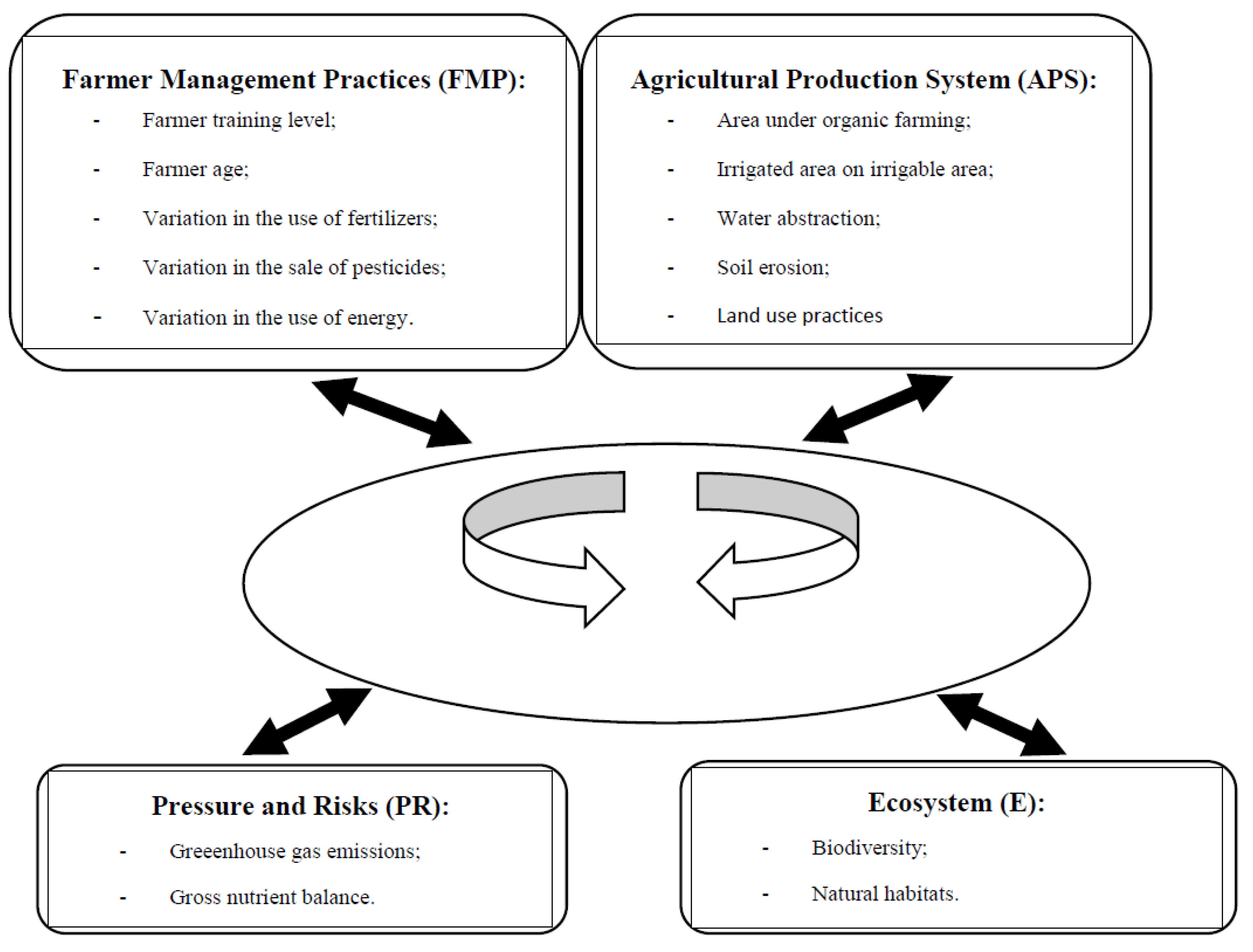
To answer the first research question (RQ1), an appropriate set of 28 AEIs was extrapolated from the Eurostat database [34]. As shown in Figure 1 and

Table 1. List of starting agri-environmental indicators (AEIs) included in this research.

Block	Definition	Unit	Year
FMP1	Farm managers with full agricultural training	Total number of holding	Var% 2013–2005
FMP2	Farm manager age	Total number of holding	Var% 2013–2005
FMP3	Consumption of nitrogen	Tonne	Var% 2016–2007
FMP4	Consumption of phosphorus	Tonne	Var% 2016–2007
FMP5	Sales of fungicides and bactericides	Kg of active ingredient	Var% 2016–2011
FMP6	Sales of herbicides, haulm destructors, and moss killers	Kg of active ingredient	Var% 2016–2011
FMP7	Sales of insecticides and acaricides	Kg of active ingredient	Var% 2016–2011
FMP8	Final energy consumption by agriculture/forestry per hectare of UAA	Kg OE/ha	Var% 2016–2007
APS1	Area under organic farming	%/UAA	2016
APS2	Irrigated area	% irrigated area/irrigable area	2013
APS3	Water abstraction for agriculture	million cubic metres	2015
APS4	Estimated soil erosion by water	% of total	2012
APS5	Estimated soil erosion by water	square km	Var% 2012–2000
APS6	Arable land	% of UAA	2013
APS7	Permanent grassland	% of UAA	2013
APS8	Permanent crops	% of UAA	2013
APS9	Bovine	% bovine/LSU	2013
APS10	Horses, asses, mules and hinnies	%/LSU	2013
APS11	Live swine domestic species	%/LSU	2013
APS12	Live sheep	%/LSU	2013
APS13	Live goats	%/LSU	2013
APS14	Live poultry	%/LSU	2013
PR1	Gross nutrient balance (phosphorus)	kg per hectare	Var% 2014–2004
PR2	Gross nutrient balance (nutrient)	kg per hectare	Var% 2014–2004
RR3	Ammonia emissions from agriculture	% of total emissions	2015
PR4	Greenhouse gas emissions from agriculture	% of total	2015
E1	Common farmland bird index [env_bio2]	base = 2000	2014
E2	Protected areas of land	%	2016

Source: Author’s elaboration of data from the EUROSTAT database. UAA: Utilised Agricultural Area; LSU: Number of Livestock Units.

, for a better understanding and integration of the full range of complex interactions between farmer training, agricultural management practices, the impact of chemical inputs on natural resources, and the equilibria of ecosystems, the AEIs were divided into the following four blocks:

(1)

Farm management practices (FMPs);

(2)

Agricultural production systems (APSs);

(3)

Pressures and risks (PRs);

(4)

Ecosystem (E).

The first block included eight driving force indicators: Two FMPs that described the changes in farmer characteristics between 2005 and 2013 (farmer training level and farmer age) and six FMPs (FMP3–FMP8) that showed the variation in management practices during the period 2007–2016 in the use of nutrients (nitrogen, phosphorus), pesticides (fungicides, bactericides, insecticides, acaricides, herbicides, haulm destructors, and moss killers), and energy. These indicators aimed to focus attention on the temporal changes in the training of farmers and their management practice decisions.

The second block of state indicators were more consistent and grouped together 14 APSs that described the effects of agriculture on the environment, for example land use practices and the estimated soil erosion by water from 2000 to 2012. In EU countries, these indicators are undergoing marked changes due to rapid shifts in consumer spending, consumer demand, and concerns over food safety and environmental impact.

In the third block, there were four PR indicators that highlighted the variation between 2004 and 2014 in the gross nutrient balance of phosphorus (PR1), nutrient (PR2), ammonia (PR3), and GHG emissions (PR4) from the agricultural sector.

Finally, in the last group, only two indicators, those that described the common farmland bird index (E1) and the incidence of the protected areas of land (E2) on the total areas, were included.

2.2. The Methodology

With reference to the research questions, given the different set of heterogeneous indicators included in the analysis, descriptive statistics and multivariate analysis were applied as they were deemed the most appropriate methods. With the first analysis, the coefficient of variation (CV), as the ratio between standard deviation and mean, was calculated to highlight the homogeneity and disparities between EU countries. Subsequently, factor analysis (FA) was adopted to identify the dominant aspects of the interactions between agricultural practices and the environment. Finally, hierarchical cluster analysis (HCA) was applied in order to regroup the 28 EU countries into “homogeneous” clusters. These analyses were carried out using the STATA programmer (Stata 12.32, software package created in 1985 by Stata Corp), which serves as an environment for the management, analysis, and graphic representation of data. Using this software, homogeneous countries were identified by arranging the various impacts of agricultural practices on the environment in a square matrix measuring (m x n), where m corresponds to the 28 EU countries and n to the temporal variation of the 28 AEIs. On the basis of this matrix, data processing was performed in two successive phases: A core FA for each aspect of the AEIs and an HCA.

FA allowed for the reduction of a significant number of variables to a meaningful, interpretable, and manageable set of factors [37]. The application of FA allowed the eigenvalues to be determined, which represent a share of the total variance. The aim of the FA is, above all, the analysis of the dependence structure, which leads to a simple description of that structure [38]. The HCA phase in contrast made use of Ward’s method of measuring the squared Euclidean distance. This method is distinct from all others since it uses an analysis of variance approach to evaluate the distances between clusters. In short, this method attempts to minimize the sum of squares (SS) of any two (hypothetical) clusters that can be formed at each step (see Ward, 1963) [39].

The hierarchical methods are often classified as agglomerative and divisive, of which the agglomerative approach has been the more popular and a large number of applications proves its practical utility; but selecting the optimal number of clusters is one of the central problems [40]. For this study, the final result was a classification “map” of EU countries, with differentiated agricultural systems. Detailed information about cluster analysis is in Appendix A.

3. Results

3.1. The Descriptive Statistical Measures of Selected AEIs

For the 28 AEIs taken into account for this study, the statistical characteristics were determined, which included the arithmetic mean, the minimum value, the maximum value, the standard deviation, and the CV. Their values are presented in

Table 2. Descriptive statistics of the country variables. Coefficient of variation (CV).

Variable	Min	Max	Std. Dev.	CV	Skewness	Kurtosis
FMP1	−76.18	300	75.50	6.19	0.0000	0.0003
FMP2	−74.2	1.17	19.12	−5.26	0.9909	0.9588
FMP3	−44.56	105.64	28.80	3.18	0.0022	0.0045
FMP4	−74.58	178.87	51.29	−9.19	0.0004	0.0016
FMP5	−45.13	1845.1	347.76	4.37	0.0000	0.0000
FMP6	−56.77	69.19	22.59	−7.31	0.0341	0.0084
FMP7	−74.5	1666.56	341.79	3.36	0.0000	0.0000
FMP8	−79.35	75.27	30.03	74.87	0.6062	0.0890
APS1	0.21	21.25	5.45	0.70	0.0334	0.5807
APS2	0	100	29.99	0.66	0.6782	0.1556
APS3	0	8282.54	1575.86	3.76	0.0000	0.0000
APS4	0	24.58	6.31	1.26	0.0007	0.0250
APS5	−86.54	62.58	27.50	−1.08	0.0865	0.0158
APS6	21	98.5	18.91	0.30	0.4439	0.8577
APS7	0	79	18.81	0.59	0.4385	0.5446
APS8	0	25	7.26	1.38	0.0015	0.1628
APS9	20.8	84	16.68	0.34	0.7935	0.7783
APS10	0.3	7.7	1.53	0.71	0.0000	0.0011
APS11	6.4	65.7	12.97	0.50	0.0302	0.0744
APS12	0.3	40.5	8.93	1.29	0.0000	0.0006
APS13	0	17.1	3.59	2.32	0.0000	0.0000
APS14	1	36.5	7.12	0.50	0.0834	0.0314
PR1	−100	100	55.92	−3.21	0.1454	0.6588
PR2	−40.91	115.79	38.40	8.89	0.0007	0.0192
PR3	78.5	99.5	6.09	0.07	0.1219	0.5158
PR4	2.6	30.8	6.29	0.56	0.0011	0.0279
E1	0	116.3	42.20	0.90	0.7179	0.0000
E2	8	38	8.51	0.43	0.0791	0.6709

. With this first analysis, the measure of the similarities/dissimilarities was conducted mainly on the basis of the values of the CV. These values show the greatest heterogeneity in final energy consumption by agriculture and forestry per hectare of the utilized agricultural area (UAA) (a −79.35:75.27 ratio between the lowest and the highest utilization) and gross nutrient balance per hectare of the UAA (−40.91:115.79). As for farmer management, the differences for farm managers with full agricultural training (−76.2 percentage variation: 300 percentage variation) and for the sales of fungicides and bactericides (−45.13 percentage variation: 1845.1 percentage variation) are also significant. This confirms, in accordance with recent studies [41,42], that holdings managed by young farmers with full agricultural training represent a significant element of the differentiation between EU countries.

Despite these dissimilarities, there were greater homogeneities between the same countries, mainly regarding the following characteristics of agricultural systems: The ammonia emissions from the agricultural sector associated with livestock production that requires large areas of land and the area of arable land with intense cattle breeding. Livestock production systems occupy around 28% of the land surface of the EU (equivalent to 65% of the agricultural land). About 18% of global GHG emissions are caused by livestock production, with the main contributors being methane (CH₄) from enteric fermentation, nitrous oxide (N₂O) from manure and fertilizer, and carbon dioxide (CO₂) [43].

Finally, it should be noted that some of the variables show excess kurtosis or skewness and, therefore, do not follow normal distributions; a fact that was taken into account when choosing the techniques to be used in the later stages of the research.

3.2. FA: Country Indicators and Agro-Environment Dimensions

The principal factors were extracted on the basis of the data reported in Table 1. FA was used to look for the dominant dimensions of the interaction between agricultural practices and the impacts on natural resources. These dominant factors adequately summarise the information contained in the original sets of indicators (RQ2: What are the information needs of farmers for the adoption of sustainable agricultural methods?). Twenty-eight eigenvalues were identified, but the first 10 together explained about 85% of the total variance (

Table 3. Total variance and percentage of individual factors. Results of factor analysis (FA).

Factor	Eigenvalue	Difference	Proportion	Cumulative
Factor1	5.29	1.39	19.03	19.03
Factor2	3.91	0.90	14.03	33.06
Factor3	3.01	0.58	10.8	43.86
Factor4	2.43	0.22	8.73	52.59
Factor5	2.21	0.49	7.95	60.55
Factor6	1.73	0.18	6.2	66.75
Factor7	1.54	0.27	5.54	72.29
Factor8	1.28	0.05	4.58	76.88
Factor9	1.23	0.18	4.41	81.29
Factor10	1.04	0.17	3.75	85.04
Factor11	0.88	0.21	3.15	88.19
Factor12	0.67	0.13	2.41	90.6
Factor13	0.54	0.00	1.94	92.54
Factor14	0.53	0.08	1.93	94.46
Factor15	0.46	0.08	1.64	96.1
Factor16	0.38	0.12	1.35	97.45
Factor17	0.26	0.11	0.93	98.39
Factor18	0.15	0.05	0.53	98.92
Factor19	0.10	0.02	0.37	99.29
Factor20	0.09	0.03	0.31	99.6
Factor21	0.06	0.03	0.21	99.81
Factor22	0.03	0.01	0.11	99.92
Factor23	0.02	0.02	0.08	100
Factor24	0.00	0.00	0.01	100
Factor25	0.00	0.00	0.00	100
Factor26	−0.00	0.00	0.01	100
Factor27	−0.00	0.00	0.02	100
Factor28	−0.00	0.00	0.03	100

The bold test indicates the factors considered in the analysis because showed eigenvalues greater than 2; The black test, from factor 6 to factor 10, indicates factors eigenvalues greater than 1. Finally, the factors (from 11 to 24), were not considered because highlight eigenvalues minor than 1.

). Attention was focused on the first five factors (about 61% of the variance) with eigenvalues greater than 2.

Table 4. Matrix of rotated first five factors loadings. The factor loadings that were smaller in absolute value than 0.45 were omitted.

Variable	Factor 1	Factor 2	Factor 3	Factor 4	Factor 5	Communalities
FMP1						0.214
FMP2		0.481			−0.479	0.750
FMP3			0.764			0.500
FMP4			0.837			0.972
FMP5						−0.995
FMP6				0.582		0.776
FMP7						0.708
FMP8				0.507		−0.236
APS1				0.454		0.535
APS2	0.464					0.327
APS3	0.689				0.541	1.105
APS4	0.541					1.412
APS5		0.614				1.987
APS6	−0.539	−0.670				−0.975
APS7		0.861				0.891
APS8	0.712					0.259
APS9		0.769				0.485
APS10			0.644			0.249
APS11		−0.686				−1.873
APS12	0.772					0.774
APS13	0.775				0.474	0.784
APS14		−0.510				0.849
PR1			0.597			0.926
PR2				0.699		1.521
PR3						1.417
PR4		0.471				0.458
E1	−0.689					−0.115
E2	0.597					0.870

shows the matrix of rotated factor loadings that represents the correlation indexes of the 28 initial AEIs, which were regrouped into four blocks, showing the first five factors. These factors represented the differentiation factors within the whole variable system in question. One factor loading greater in absolute value than 0.5 is considered very significant [44]. The derived rotated 5-factor structure is shown in Table 4, with the omission of factor loadings that were smaller in absolute value than 0.45. Concerning the interpretation of the factors, Table 4 shows that the first three factors were essentially related to three categories of variables: farmer management, agricultural production systems, and pressures and risks. It can be observed that the variables from the ecosystem category were not represented in any of the key factors. The analysis of the key factors demonstrated a high level of heterogeneity among EU countries.

Factor 1 “Pastoral system with a negative effect on the farmland bird index”: The first factor (more than 19% of the explained variance) (Greece, Portugal, Slovenia, Cyprus, Croatia) was characterised by a high percentage on the LSU (Number of Livestock Units) of live goats (+0.78) and sheep (+0.77), with strong positive correlations with the permanent crops variable (+0.71) and negative correlations with the common farmland bird index (−0.69). A negative correlation (−0.54) can also be noted with arable land, which was an expected result.

Factor 2 “Extensive livestock system with a negative effect on soil and air”: 14% of the explained variance (Ireland, Luxembourg, the UK, Slovenia). This factor was associated with a high percentage of permanent grassland (+0.86) and a large percentage of bovines on the LSU (+0.77). It was also related positively to estimated soil erosion by water (+0.61). Therefore, countries with a high score on this factor are certainly poor, have a permanent grassland, and a traditional and essential agricultural system based on animal husbandry with high GHG emissions from agriculture (+0.47).

Factor 3 “Intensive agricultural system with a positive variation of phosphorus balance”: (10.8% of the explained variance) expressed high percentage variation (2016–2007) in the tonnes of phosphorus and nitrogen used, which is associated with a high percentage on the LSU of horses, asses, mules, and hinnies and consequently a positive percentage variation (2014–2004) in the gross nutrient balance (phosphorus). The countries (Bulgaria, Ireland, Malta, Slovenia) with a high score on this factor have a large number of holdings with farmers with full agricultural training.

Factor 4 “Agricultural system with a positive variation in the nutrient balance”: (8.7% of the explained variance) (Austria, Hungary, Latvia, the Czech Republic) is associated with a positive percentage variation in the sale of herbicides, haulm destructors, and moss killers (+0.58) and is positively correlated with the positive percentage variation in the final energy consumption by the agriculture/forestry sector per hectare of the UAA (+0.51) and in the high percentage of area under organic farming (+0.45).

Factor 5 “Agricultural system with high water abstraction for agriculture”: (about 8% of the explained variance) (Greece, Romania, Poland, Bulgaria) shows, on the one hand, a negative correlation with farm manager age (–0.48) and, on other hand, a positive correlation with the percentage of live goats on the LSU (+0.48) and with the estimated soil erosion by water (+0.57).

3.3. Which Countries Have the Greatest Similarities? A Discussion of the HCA

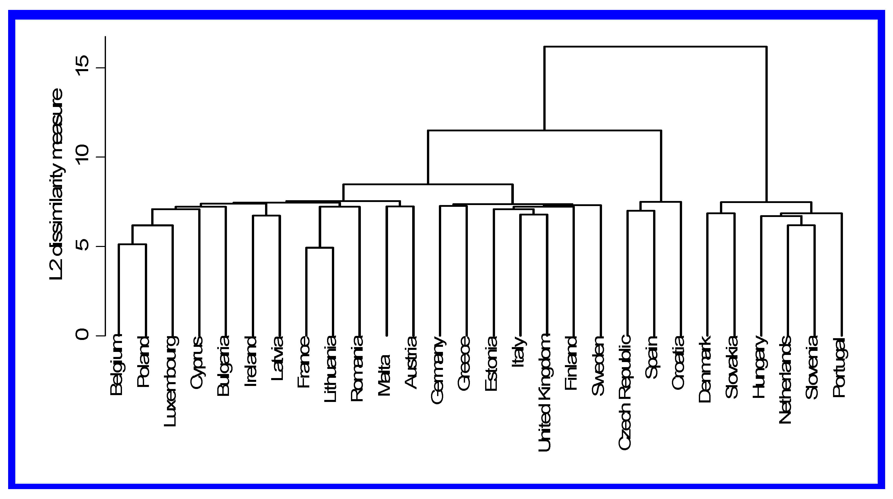
Following the FA, HCA was used to look for groups of EU countries with similar levels of linkage between agricultural activities and environmental impacts. The resulting dendrogram provides a visual interpretation of the procedure and the findings of the hierarchical agglomeration for the observed 28 EU countries, from left to right (Figure 2). The first cluster comprised a great number of countries (12.4%), especially from the north of the EU; the second group contains 7 EU countries, the third group 3 EU countries, and the fourth group 6 EU countries. It can be observed that the 28 EU countries did not form a homogeneous group in terms of the relationship between agricultural practices and environmental impacts. Indeed, four groups could be distinguished (Figure 3).

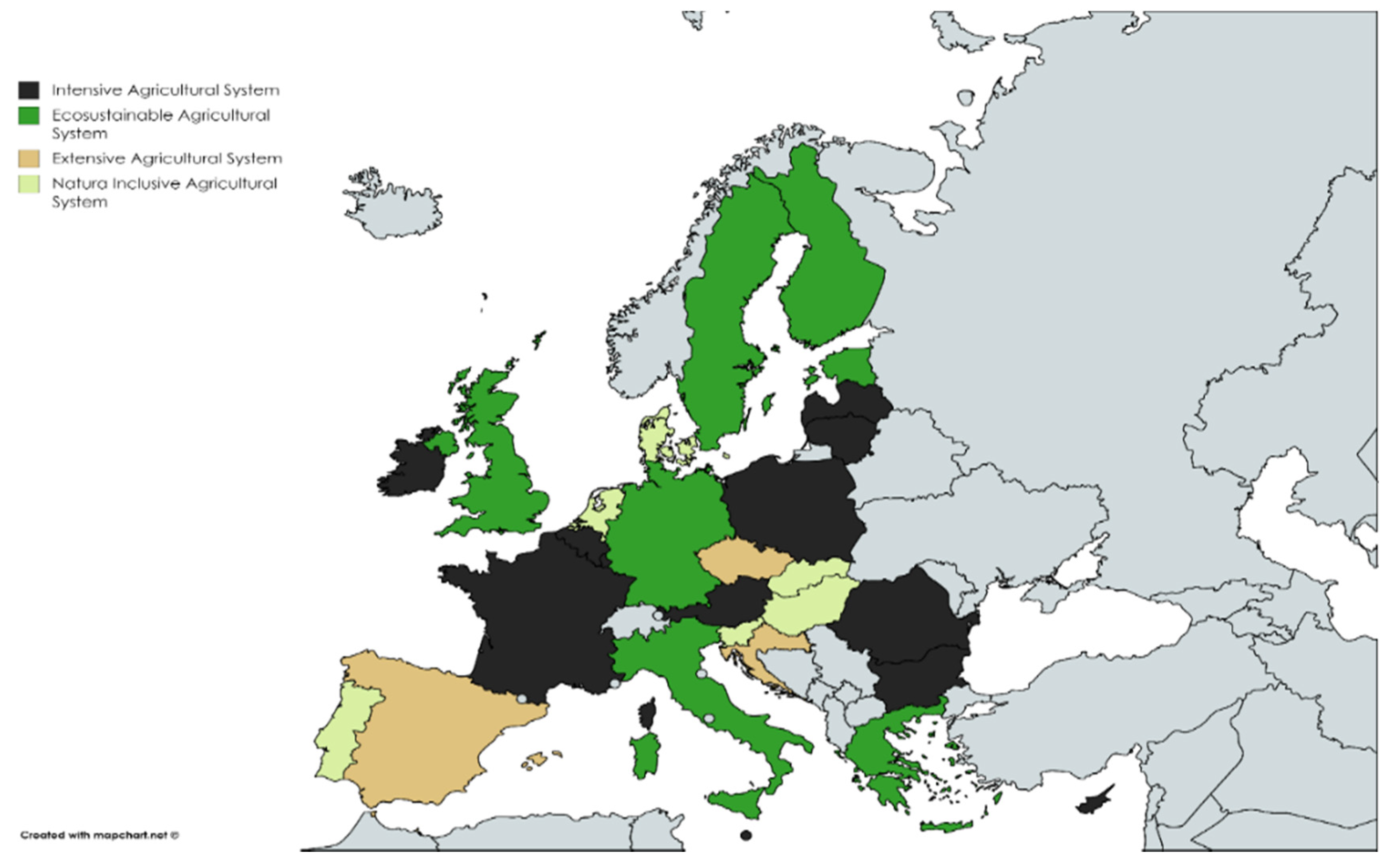
The “homogenous” clusters are mapped in Figure 3.

Cluster 1: “Intensive agricultural system”: This first group was the largest. It was made up of 12 countries, situated mainly in Northern and Central Europe (Figure 3). The main characteristic of this cluster was the high percentage of bovines on the LSU. Luxembourg and Ireland showed the highest value, 84% and 82.2%, respectively. The livestock agricultural system, as is well-known, causes high emissions of ammonia and a high consumption of water [32,45,46,47]. Compared to the other three groups, the average percentage of bovines on the LSU for each country was about 54% versus 50% for the second group, 42% for the third group, and 44% for the last group. The agricultural sector of this cluster utilized 43% of the community arable land and was responsible for 43% of the total ammonia emissions and 50% of the GHG emissions (

Table 5. Mean of each cluster and mean of the 28 EU countries.

Cluster	FMP1	FMP2	FMP3	FMP4	FMP5	FMP6	FMP7
Cluster 1	27.38	−36.71	22.17	14.48	23.88	−5.27	34.90
Cluster 2	−6.69	−34.22	0.33	−16.87	277.99	3.75	327.12
Cluster 3	0.49	−38.83	−7.70	−29.90	8.04	−2.22	8.23
Cluster 4	9.74	−36.92	1.33	−20.37	−4.56	−7.16	19.46
Mean 28 EU countries	12.20	−36.36	9.04	−5.58	79.62	−3.09	101.79
Cluster	FMP8	APS1	APS2	APS3	APS4	APS5	APS6
Cluster 1	5.83	6.00	48.58	280.50	4.51	−19.42	62.53
Cluster 2	−13.64	11.05	41.04	1183.22	5.63	−33.31	64.29
Cluster 3	−3.47	9.51	35.42	18.03	5.52	−29.46	58.60
Cluster 4	7.86	6.61	49.24	5.69	4.99	−26.66	61.13
Mean 28 EU countries	0.40	7.77	45.43	419.17	5.00	−25.52	62.25
Cluster	APS7	APS8	APS9	APS10	APS11	APS12	APS13
Cluster 1	31.99	4.50	53.50	2.43	23.95	5.53	1.53
Cluster 2	30.23	5.44	49.54	2.17	21.41	11.47	2.63
Cluster 3	33.67	7.67	41.60	1.53	31.80	7.17	0.90
Cluster 4	33.37	5.35	44.08	1.92	31.47	4.37	0.63
Mean 28 EU countries	32.03	5.26	49.22	2.16	25.77	6.94	1.55
Cluster	APS14	PR1	PR2	PR3	PR4	E1	E2
Cluster 1	12.93	−14.16	7.75	92.77	13.16	49.22	18.67
Cluster 2	12.74	−14.69	−6.88	91.07	8.81	56.17	16.43
Cluster 3	16.93	−9.09	−0.08	90.67	9.20	27.07	26.00
Cluster 4	17.50	−31.34	12.72	89.63	11.18	40.73	21.83
Mean 28 EU countries	14.29	−17.43	4.32	91.45	11.23	46.76	19.57

).

Cluster 2: “Eco-sustainable agricultural system”: There were 7 countries in the second cluster: Germany, Greece, Estonia, Italy, the United Kingdom, Finland, and Sweden. In this second cluster, there were three countries (Estonia, Italy, and Sweden) of the five countries (Austria, the Czech Republic, Estonia, Italy, and Sweden) that had the largest area of land under organic farming in the total area of the EU. Indeed, the average percentage for these counties was 11.05. (Table 5). Organic farming, when compared to conventional systems, is more sustainable because it generates less soil erosion, more water conservation, and improved soil organic matter and biodiversity compared to conventional systems [48,49].

Cluster 3: “Extensive agricultural system”: There were only three countries in the third group: the Czech Republic, Spain, and Croatia. This cluster showed the highest average percentage of protected areas (26%) compared to the other three groups. The high presence of permanent grassland (almost 34% against an average of 19.6% in all 28 EU countries) is an ideal measure for the prevention of soil erosion from wind and water [50,51].

Cluster 4: “Nature inclusive agricultural system”: This fourth and final cluster contained six countries: Denmark, Hungary, the Netherlands, Portugal, Slovenia, and Slovakia. These countries, especially the Netherlands and Slovenia, in the period between 2004 and 2014, on one hand decreased the use of P-fertiliser per hectare of UAA, which, as is well-known, can change the botanical composition of grassland by favouring particular species over others. However, these countries also registered an increase in the sale of insecticides and acaricides and in the final consumption of energy. In the last 10 years, these countries adopted a more sustainable form of agriculture that minimizes negative ecological impacts, maximizes positive impacts, and, at the same time, benefits from natural processes [52].

4. Discussion and the Environmental Policy Implications

The application of descriptive statistics and multivariate analyses to the 28 EU countries led to a new and more accurate classification of the member states into four “homogeneous” territorial agricultural systems (Figure 3). It also led to the creation of a new tool for policymakers to aid them in developing environmental programmes for the future CAP post 2020 (2021–2027) and to increase the knowledge of farmers (How can policymakers define different incentives that could push farmers to adopt more sustainable agricultural production methods?).

In particular, with the aid of the four groups of AEIs extrapolated from the EUROSTAT (Statistical Office of the European Communities) database and with the research questions derived mainly from the previous literature, it was possible to highlight the difficult trade-off between the increase in the intensification of agricultural production and the degradation of natural resources.

Initially, by using the CV, the differences and the similarities of each EU country were measured, with respect to each indicator. This analysis highlighted the existence of large disparities between the EU countries in relation to the final energy consumption of agriculture and forestry per hectare of the UAA (a −79.35:75.27 ratio between the lowest and highest utilization) and the gross nutrient balance per hectare of the UAA (−40.91:115.79). On the one hand, the maximum increase of direct electric and fuel energy consumption (KgOE), from 2006 to 2016, was registered by Romania (+75.27 KgOE/ha). On the other hand, the maximum decrease was recorded in Greece (−79.35 KgOE/ha). Other countries with a consistent increase were Hungary, Cyprus, Austria, and the Czech Republic. In contrast, the more “virtuous” countries were Sweden, Ireland, Bulgaria, and Lithuania. These disparities were due mainly to the degree of cultivation intensity, the heating of livestock stables, and the training level and age of farmers. In relation to age, older farmers were more likely to adopt more traditional farming systems with a higher consumption of energy. For this reason, in this study, to assess energy consumption, the data was linked to farm management and land use practices.

In contrast, there were some similarities regarding ammonia emissions from the agricultural sector, arable land coverage, and the intensity of cattle breeding. In particular, GHG emissions from livestock production were closer to 51% of global GHG emissions [32,44,45,46,47]. These negative effects of agricultural practices on the environment have a high correlation, in accordance with recent studies [32,33], with an increase in almost all EU countries in livestock production, due, in the main part, to an increase in meat consumption. The latter can be attributed to a lack of essential information for consumers (sustainable education) and to an increase in consumer income in all EU countries.

Following this, an analysis of the territorial similarities of EU countries was carried out by examining the principle factors brought to light by the statistical analysis. This allowed the identification of the five most important factors and agricultural phenomena: “Pastoral system with a negative effect on farmland bird index”; “Extensive livestock system with a negative effect on soil and air”; “Intensive agricultural system with a positive variation of phosphorus balance”; “Agricultural system with a positive variation in nutrient balance”; and “Agricultural system with high water abstraction for agriculture”.

Based on the findings of this study, it is possible conclude that the linkages between agricultural activities and environmental impacts are different among the 28 EU countries. Indeed, on the one hand, the results of the HCA clearly show that the first group of EU countries (in the centre and north of the EU), labelled “Intensive agricultural system” registered a high impact on natural resources (air and soil) and a high use of water. This result provides evidence, in accordance with other recent studies [32,33], of a strong relationship between GHG emissions and the livestock sector. In these countries, for more environmentally-friendly and sustainable agriculture activities, any measures taken should aim to limit the intensity of livestock farming to promote sustainable production and to limit resource use (soil and water). In this regard, several studies have shown that a full and effective implementation of environmentally-friendly farming practices (EFFPs) goes far beyond financial support and needs to be based on a change in the behaviour and intentions of farmers [53,54,55,56,57].

On the other hand, the three clusters labelled: “Eco-sustainable agricultural system”, “Extensive agricultural system”, and “Nature inclusive agricultural system” require action for the conservation of the “diversity” of rural and agricultural systems. For this purpose, it is essential to implement in these EU countries, direct payments, and the less favoured area scheme with the aim of both preserving the extensive grazing systems and the traditional rural landscapes and avoiding land abandonment and the disappearance of these landscapes. Moreover, the necessity to comply with good agricultural and environmental standards in order to receive the full-decoupled direct payment, and the implementation of agro-environmental payment schemes to encourage farmers to carry out agricultural activities favourable to the maintenance of the countryside, has positively influenced landscape provision. It is important to observe that, from the analysis, it emerged that the similarity between agricultural systems is not linked to geographical position or environmental contexts but to the characteristics of crops and production processes. In each of the groups created by the analysis, a characterizing or unifying element was identified. For example, the Eco-sustainable agricultural system was characterised by the prevalence of organic farming methods, a factor that united the countries of this second cluster. In another case, it was a particularly polluting aspect of the production process—the presence of a livestock dominated by bovines—that characterised the numerous and diverse agricultural systems of group 1 (Intensive agricultural system) and made them very intensive due to their high consumption of water and the significant emissions of climate-altering gases, in particular ammonia. For the next long-term EU budget 2021–2027, the Commission has proposed to modernize and simplify the CAP, stipulating that at least 30% of each rural development national allocation be dedicated to environmental and climate measures. A total of 40% of the CAP’s overall budget is expected to contribute to climate action.

In conclusion, the results of the analysis are in line with other studies [32,33,42,58] that have applied multivariate analysis and confirm that policy design should not consider the EU context as a whole. On the contrary, it should take into account the land-use practices and the productive particularities, as well as the temporal trends in the use of natural resources and chemical inputs (fertilizers and pesticides). According to the study findings, policymakers could target specific measures to incentivize good agricultural practices on the basis of the different realities in the four groups of countries at the EU level. These targeted measures could lead to farms being run by individuals with greater training in order to achieve the sustainable development of agricultural production methods. This will allow policymakers and those involved in local government to have enhanced and more effective tools, as required by the new CAP for the next operational period (2021–2027), for a more exact and better monitoring of the impact of agricultural practices and production on natural resources.

The results of the research assess the viability of the different actions of the CAP on the basis of the differences and analogies in agricultural impact on the environment among EU countries. However, countries with similar, high impact agricultural practices and production methods might be steered towards sustainable intensification with similar interventions. Therefore, the findings of this analysis and its follow up could be useful to policymakers generally, in order to define tools that guide producers towards more sustainable production methods; an objective pursued by the CAP with increasing efforts. The EU needs high-quality AIE elaboration to design, implement, and monitor policies that benefit all of its citizens. Furthermore, in order to highlight some of the main differences between the results of the present study and previous research, a number of recent studies were scrutinised. For example, on the one hand, there is much agreement between the intensity of nitrogen input in both arable and grassland systems and the classification of countries, such as Romania, Bulgaria, and Poland, as a group with high intensity agricultural systems (45–47). On the other hand, the results are in line with another recent study [59] that classified some countries from Central and Eastern Europe (Slovakia and the Czech Republic) as a group with the highest level of sustainability, therefore mirroring this study’s classification: “Nature inclusive agricultural system”.

The main novelty of this study is that in the literature there are very few publications about the geo-spatialised classification of EU countries that offer data on the evolution of the impacts of agricultural practice and production on the environment. However, a limitation is that the research used a selection of blocks of indicators, whereas a wider classification of variables could lead to a more comprehensive assessment of the effects of different agricultural practices on the environment. A final remark: Although the statistical techniques that were used in the paper were able to respond to the goals of this research, it would be an interesting and promising task to conduct further analysis that aims to compare results from different classification techniques.

References

- EEA. Food in a Green Light. A System Approach to Sustainable Food; Environmental, European Environment Agency: Copenhagen, Denmark, 2017.
- EEA. Down to Earth: Soil Degradation and Sustainable Development in Europe; Environmental, European Environment Agency: Copenhagen, Denmark, 2000; Volume 16, pp. 1–32.
- Girardin, P. Indicators: Tools to evaluate the environmental impacts of farming systems. J. Sustain. Agric. 2012, 13, 5–21. [Google Scholar] [CrossRef]
- Crabtree, J.R.; Brouwer, F.M. Discussion and conclusions. In Environmental Indicators and Agricultural Policy; Brouwer, F.M., Crabtree, J.R., Eds.; CAB International: Wallingford, UK, 1999; pp. 279–285. [Google Scholar]
- OECD. Environmental Indicators for Agriculture. Methods and Results; OECD Publications: Paris, France, 2001; Volume 3, p. 409. [Google Scholar]
- Mitchell, G.; May, A.; Mc Donald, A. PICABUE: A methodological framework for the development of indicators of sustainable development. Int. J. Sustain. Dev. World 1995, 2, 104–123. [Google Scholar] [CrossRef]
- Bossel, H. Assessing viability and sustainability: A systems-based approach for deriving comprehensive indicator sets. Conserv. Ecol. 2001, 5, 12. [Google Scholar] [CrossRef]
- Jollands, N. How to aggregate sustainable development indicators: A proposed framework and its application. Int. J. Agric. Resour. Gov. Ecol. 2006, 5, 18–34. [Google Scholar] [CrossRef]
- Cloquell-Ballester, V.A.; Cloquell-Ballester, V.A.; Monterde-Diaz, R.; Santamarina-Siurana, M.C. Indicators validation for the improvement of environmental and social impact quantitative assessment, environmental. Impact Assess. Rev. Environ. 2006, 26, 79–105. [Google Scholar] [CrossRef]
- MAFF (Ministry of Agriculture, Fisheries, Food). Towards Sustainable Agriculture (A Pilot Set of Indicators); MAFF Publication: London, UK, 2000.
- Wascher, D.W. Agri-environmental Indicators for Sustainable Agriculture in Europe; European Centre for Nature Conservation: Tilburg, The Netherlands, 2000. [Google Scholar]
- Chen, Q.; Sipiläinen, T.; Sumelius, J. Assessment of agri-environmental externalities at regional levels in Finland. Sustainability 2014, 6, 3171–3191. [Google Scholar] [CrossRef] [Green Version]
- Borrelli, P.; Panagos, P.; Montanarella, L. New insights into the geography and modelling of wind erosion in the European agricultural land. Application of a spatially explicit indicator of land susceptibility to wind erosion. Sustainability 2015, 7, 8823–8836. [Google Scholar] [CrossRef] [Green Version]
- Nevado-Peña, D.; López-Ruiz, V.-R.; Alfaro-Navarro, J.-L. The effects of environmental and social dimensions of sustainability in response to the economic crisis of European cities. Sustainability 2015, 7, 8255–8269. [Google Scholar] [CrossRef] [Green Version]
- Peano, C.; Tecco, N.; Dansero, E.; Girgenti, V.; Sottile, F. Evaluating the sustainability in complex agri-food systems: The SAEMETH framework. Sustainability 2015, 7, 6721–6741. [Google Scholar] [CrossRef] [Green Version]
- Janković Šoja, S.; Anokić, A.; Bucalo Jelić, D.; Maletić, R. Ranking EU countries according to their level of success in achieving the objectives of the sustainable development strategy. Sustainability 2016, 8, 306. [Google Scholar] [CrossRef] [Green Version]
- Rigby, D.; Woodhouse, P.; Young, T.; Burton, M. Constructing a farm level indicator of sustainable agriculture practice. Ecol. Econ. 2001, 39, 463–478. [Google Scholar] [CrossRef]
- Van der Werf, H.M.G.; Petit, J. Evaluation of the environmental impact of agriculture at the farm level: A comparison and analysis of 12 indicator-based methods. Agric. Ecosyst. Environ. 2002, 93, 131–145. [Google Scholar] [CrossRef]
- Yli-Viikari, A.; Hietala-Koivu, R.; Huusela-Veistola, E.; Hyvönen, T.; Perälä, P.; Turtola, E. Evaluating agri-environmental indicators (AEIs)-Use and limitations of international indicators at national level. Ecol. Econ. 2007, 7, 150–163. [Google Scholar] [CrossRef]
- Engström, R.; Nilsson, M.; Finnveden, G. Which environmental problems get policy attention? Examining energy and agricultural sector policies in Sweden. Environ. Impact Assess. Rev. 2008, 28, 241–255. [Google Scholar]
- Beckmann, V.; Eggers, J.; Mettepenningen, E. Deciding how to decide on agri-environmental schemes: The political economy of subsidiarity, decentralisation and participation in the European Union. J. Environ. Plan. Manag. 2009, 52, 689–716. [Google Scholar] [CrossRef]
- Gottero, E.; Cassatella, C. Landscape indicators for rural development policies. Application of a core set in the case study of Piedmont Region. Environ. Impact Assess. Rev. 2017, 65, 75–85. [Google Scholar] [CrossRef]
- Scherer, L.A.; Verburg, P.H.; Schulp, C.J.E. Opportunities for sustainable intensification in European agriculture. Glob. Environ. Chang. 2018, 48, 43–55. [Google Scholar] [CrossRef]
- Payraudeau, S.; van der Werf, H.M.G. Environmental impact assessment for a farming region: A review of methods. Agric. Ecosyst. Environ. 2005, 107, 1–19. [Google Scholar] [CrossRef]
- Dent, J.B.; Edwards-Jones, G.; McGregor, M.J. Simulation of ecological, social and economic factors in agricultural systems. Agric. Syst. 1995, 49, 337–351. [Google Scholar] [CrossRef]
- Gallopin, G.C. Indicators and their use: Information for decision-making. In Sustainability Indicators: A Report on the Project on Indicators of Sustainable Development; Billhartz, S.B., Matravers, R., Eds.; John Wiley and Sons: Chichester, UK, 1997; pp. 13–27. [Google Scholar]
- Molden, D.J.; Sakthivadivel, R.; Perry, C.J.; de Fraiture, C.; Kloezen, W.H. Indicators for Comparing Performance of Irrigated Agricultural Systems; IWMI Research Report; International Water Management Inst.: Colombo, Sri Lanka, 1998; Volume 20, p. 26. [Google Scholar]
- Deller, S.; Tsai, T.; Marcouiller, D.; English, D. The role of amenities and quality of life in rural economic growth. Am. J. Agric. Econ. 2001, 83, 352–365. [Google Scholar] [CrossRef]
- Tabachnick, B.; Fidell, L. Using Multivariate Statistics; Pearson/Allyn and Bacon: Boston, MA, USA, 2005. [Google Scholar]
- Madu, I. The underlying factors of rural development patterns in the Nsukka region of Southeastern Nigeria. J. Rural Commun. Dev. 2007, 2, 110–122. [Google Scholar]
- Hossain, M.; Begum, E.; Papadopoulou, E. Factors of rural development driver in Southeastern Bangladesh. Am. J. Rural Dev. 2015, 3, 3440. [Google Scholar]
- Fanelli, R.M. The interactions between the structure of the food supply and the impact of livestock production on the environment. A multivariate analysis for understanding the differences and the analogies across European union countries. Calitatea 2018, 19, 131–139. [Google Scholar]
- Fanelli, R.M. The (un)sustainability of the land use practices and agricultural production in EU countries. Int. J. Environ. Stud. 2019, 2, 273–294. [Google Scholar] [CrossRef]
- European Commission, Eurostat. Agri-environmental Indicators. 2018. Available online: http://ec.europa.eu/eurostat/web/agri-environmental-indicators/indicators (accessed on 12 June 2019).
- Felici, F. Tools and Methods for Sustainable Development of the Rural Territories. Rural Innova Interreg IIIC South; IRPET: Firenze, Italy, 2006; Available online: http://www.irpet.it/index.php?page=pubblicazione&pubblicazione_id=148.
- Simoncini, R. Definition of a common European analytical framework for the development of local agri-environmental programmes for biodiversity and landscape conservation (AEMBAC). In 5th Framework Contract Ref: QLRT-1999–31666; Work package 6-Report; IUCN-ERO: Brussels, Belgium, 2002; unpublished. [Google Scholar]
- Myers, J.H.; Mullet, G.M. Managerial Applications of Multivariate Analysis in Marketing; American Marketing Association: Chicago, IL, USA, 2003. [Google Scholar]
- Balicki, A. Statystyczna Analiza Wielowymiarowa i jej Zastosowania Społeczno-Ekonomiczne; Wydawnictwo Uniwersytetu Gdańskiego: Gdańsk, Poland, 2009. [Google Scholar]
- Ward, J.H. Hierarchical grouping to optimize an objective function. J. Am. Stat. Assoc. 1963, 58, 236–244. [Google Scholar] [CrossRef]
- Everitt, B.S.; Landau, S.; Leese, M. Cluster Analysis; Edward Arnold: London, UK, 2001. [Google Scholar]
- Fanelli, R.M. Rural small and medium enterprises development in Molise (Italy). Eur. Countrys. 2018, 10, 566–589. [Google Scholar] [CrossRef] [Green Version]
- D’Amico, M.; Coppola, A.; Chinnici, G.; Di Vita, G.; Pappalardo, G. Agricultural systems in the European Union: An analysis of regional differences. New Medit. 2013, 12, 28–34. [Google Scholar]
- FAO. The State of Food and Agriculture. Food Aid for Food Security; FAO Publications: Rome, Italy, 2006; pp. 1–168. [Google Scholar]
- Hair, J.F.; Anderson, R.E.; Tatham, R.L.; Black, W.C. Multivariate Data Analysis; Prentice Hall International: Upper Saddle River, NJ, USA, 1998. [Google Scholar]
- Pérez-Soba, M.; Elbersen, B.; Kempen, M.; Braat, L.; Staristky, I.; Wijngaart, R.; van der Kaphengst, T.; Andersen, E.; Germer, L.; Smith, L.; et al. Agricultural Biomass as Provisioning Ecosystem Service: Quantification of Energy Flows; EUR 27538 EN; Publications Office of the European Union: Luxembourg, 2015. [Google Scholar]
- Malek, Ž.; Verburg, P. Mediterranean land systems: Representing diversity and intensity of complex land systems in a dynamic region. Landsc. Urban Plan. 2017, 165, 102–116. [Google Scholar] [CrossRef] [Green Version]
- Levers, C.; Butsic, V.; Verburg, P.H.; Müller, D.; Kuemmerle, T. Drivers of changes in agricultural intensity in Europe. Land Use Policy 2016, 58, 380–393. [Google Scholar] [CrossRef] [Green Version]
- Condron, L.M.; Cameron, K.C.; Di, H.J.; Clough, T.J.; Forbes, E.A.; McLaren, R.G.; Silva, R.G. A comparison of soil and environmental quality under organic and conventional farming systems in New Zealand. J. Agric. Res. 2000, 43, 443–466. [Google Scholar] [CrossRef]
- Bai, Z.; Caspari, T.; Gonzalez, M.R.; Batjes, N.H.; Mäder, P.; Bünemann, E.K.; de Goede, R.; Brussaard, L.; Xu, M.; Ferreira, C.S.S.; et al. Effects of agricultural management practices on soil quality: A review of long-term experiments for Europe and China. Agric. Ecosyst. Environ. 2018, 265, 1–7. [Google Scholar] [CrossRef]
- Lewell, C.; Meusburger, K.; Brodbeck, M.; Bänninger, D. Methods to describe and predict soil erosion in mountain regions. Landsc. Urban Plan. 2008, 88, 46–53. [Google Scholar] [CrossRef]
- Muhammed, S.E.; Coleman, K.; Wu, L.; Tipping, E.; Whitmore, A.P. Impact of two centuries of intensive agriculture on soil carbon, nitrogen and phosphorus cycling in the UK. Sci. Total Environ. 2018, 634, 1486–1504. [Google Scholar] [CrossRef]
- Sanders, M.; Westerink, J. Op Weg Naar Een Natuurinclusieve Duurzame Landbouw; Alterra Wageningen UR: Wageningen, The Netherlands, 2015. [Google Scholar]
- Upadhyay, B.M.; Young, D.L.; Wang, H.H.; Wandschneider, P. How do farmers who adopt multiple conservation practices differ from their neighbors? In Proceedings of the AAEA and WAEA, Annual Meeting, Long Beach, CA, USA, 28–31 July 2002; p. 21. [Google Scholar]
- Läpple, D. Adoption and abandonment of organic farming: An empirical investigation of the Irish drystock sector. J. Agric. Econ. 2010, 61, 697–714. [Google Scholar] [CrossRef]
- Yiridoe, E.K.; Atari, D.O.A.; Gordon, R.; Smale, S. Factors influencing participation in the Nova Scotia environmental farm plan program. Land Use Policy 2010, 27, 1097–1106. [Google Scholar] [CrossRef]
- Nyanga, P.H. Factors influencing adoption and area under conservation agriculture: A mixed methods approach. Sustain. Agric. Res. 2012, 1, 27. [Google Scholar] [CrossRef] [Green Version]
- Teklewold, H.; Kassie, M.; Shiferaw, B. Adoption of multiple sustainable agricultural practices in rural Ethiopia. J. Agric. Econ. 2013, 64, 597–623. [Google Scholar] [CrossRef]
- Serrao, A. A comparison of agricultural productivity among European Countries. New Medit. 2003, 1, 14–20. [Google Scholar]
- Nowak, A.; Krukowski, A.; Różańska-Boczula, M. Assessment of sustainability in agriculture of the European union countries. Agronomy 2019, 9, 890. [Google Scholar] [CrossRef] [Green Version]
Figure 1.
The four blocks of agri-environmental indicators considered. Source: Author’s processing of information from the EUROSTAT (Statistical Office of the European Communities) database.
Figure 2.
Dendrogram by Ward’s method.
Figure 3.
“Homogenous” European Union (EU) countries groups.