
Study of the Urban Heat Island (UHI) Using Remote Sensing Data/Techniques: A Systematic Review


1
Department of Geosciences, Environment and Land Planning, Faculty of Sciences, University of Porto, Rua Campo Alegre, 687, 4169-007 Porto, Portugal
2
Earth Sciences Institute (ICT), Pole of the FCUP, University of Porto, 4169-007 Porto, Portugal
3
Centro de Investigação de Montanha (CIMO), Campus de Santa Apolónia, Instituto Politécnico de Bragança, 5300-253 Bragança, Portugal
*
Author to whom correspondence should be addressed.
Environments 2021, 8(10), 105; https://0-doi-org.brum.beds.ac.uk/10.3390/environments8100105
Submission received: 22 August 2021
/
Revised: 21 September 2021
/
Accepted: 5 October 2021
/
Published: 9 October 2021
Abstract
:Urban Heat Islands (UHI) consist of the occurrence of higher temperatures in urbanized areas when compared to rural areas. During the warmer seasons, this effect can lead to thermal discomfort, higher energy consumption, and aggravated pollution effects. The application of Remote Sensing (RS) data/techniques using thermal sensors onboard satellites, drones, or aircraft, allow for the estimation of Land Surface Temperature (LST). This article presents a systematic review of publications in Scopus and Web of Science (WOS) on UHI analysis using RS data/techniques and LST, from 2000 to 2020. The selection of articles considered keywords, title, abstract, and when deemed necessary, the full text. The process was conducted by two independent researchers and 579 articles, published in English, were selected. Qualitative and quantitative analyses were performed. Cfa climate areas are the most represented, as the Northern Hemisphere concentrates the most studied areas, especially in Asia (69.94%); Landsat products were the most applied to estimates LST (68.39%) and LULC (55.96%); ArcGIS (30.74%) was most used software for data treatment, and correlation (38.69%) was the most applied statistic technique. There is an increasing number of publications, especially from 2016, and the transversality of UHI studies corroborates the relevance of this topic.
1. Introduction
Urbanization is an anthropic alteration that generates modifications in surface materials due to vegetation suppression, albedo variation, and soil sealing, influencing the local energy balance, contributing to the formation of the Urban Heat Island (UHI) [1]. This effect is a consequence of the greater absorption of electromagnetic energy and the slow cooling of urbanized surfaces compared to surrounding areas with the presence of vegetation [2,3].
This local dynamic contributes to an increase in surface temperature, with a subsequent reduction in relative humidity and latent heat, and an intensification of sensible heat. The main causes of UHI formation are: (i) the ability of building materials to store heat; (ii) anthropogenic heat production; (iii) alteration and minimization of wind speed as a function of surface roughness; and (iv) increased absorption of solar radiation from lower albedo surfaces, among others [4,5,6,7].
Due to the relevance of the topic, studies focusing on understanding the causes and effects of UHI are increasing, including the analysis of the variability in air temperature in urbanized areas and its underlying mechanisms [8,9,10,11]. Voogt and Oke (2003) [12] suggested a sub-classification analogous to UHI, called Surface Urban Heat Island (SUHI) which, in addition to studying surface temperature differences between urban and rural areas, also addresses temporal variability [13]. In this review, considering that not all the papers reviewed made the distinction between UHI and SUHI, the term UHI will be mentioned in the broad sense, and in the case of studies dealing with surface temperature, it assumes that the study focuses on SUHI.
The most recurrent impacts associated with this effect are: (i) influence on the local microclimate; (ii) thermal discomfort; (iii) impacts on public health; and (iv) changes in hydrological behavior, with a displacement of water masses, for example [4,5,6,7]. UHI and SUHI combined with natural phenomena, such as Heat Waves (HWs), can potentiate the impacts on human health, culminating in increased mortality [14]. Climate change will most likely generate an increase in air temperatures, raising the negative effects of UHI and SUHI, and thus demanding climate-resilient cities that can accurately analyze and promote urban planning solutions to mitigate this effect [15,16,17,18].
During the morning period, the SUHI presents great amplitude and variable behavior, especially in urbanized areas. In these same areas, the UHI presents lower temperatures when compared to those with the presence of vegetation, due to the amount of mass per unit area for heating, i.e., places with fewer horizontal and vertical constructions will need less time to heat (Figure 1) [19,20,21,22].
In addition, there is an influence regarding the thermal properties of the constituent materials and their arrangement, which can generate shading effects and corroborate to the local heat exchange characteristics: the more heterogeneous their composition, the more complex the local heating and cooling relationship (as in the case of civil constructions). In urban areas, SUHI gains intensity around noon, and during the night, urban areas retain more heat due to the thermal behavior of buildings, surface materials, and areas that have reduced view of the skydome/hemisphere, as a function of lower Sky View Factor (SVF) (Figure 1) [19,20,21,22].
There are several techniques to study the thermal behavior of a site, such as Remote Sensing (RS) [23], data from fixed meteorological stations, data from qualified entities, in situ campaigns with portable thermal cameras, etc. Some studies adopt more than one of the aforementioned data sources to complement the information, both at the atmospheric and surface-level (UHI and SUHI, respectively). This variety of sources allows the access to diurnal and/or nocturnal data and in different seasons of the year, although the effect is more intense in summer and winter [19,20,21,22].
From the RS data, it is possible to compute the Land Surface Temperature (LST), a relevant variable that can be used to determine the radiative load of the earth’s surface. It conducts longwave radiation and turbulent heat fluxes between the earth and the atmosphere, i.e., it is a variable in the physics of local and global surface processes, linked to radiative, latent, and sensible heat fluxes at the interface with the surface, allowing analyses of warming trends at the earth’s surface [24,25,26,27].
The LST, also known as radiometric or “skin” temperature, refers to the direct measurement of the earth’s surface temperature. Unlike the measurements taken by meteorological stations that record the temperature near the surface, the LST allows for a more detailed scale of analysis: in areas of dense vegetation it will represent the temperature of the leaves of the canopy; in areas of sparse vegetation the temperature will correspond to the whole canopy, subsurface (limbs, branches, etc.), and the ground surface; and on the bare ground it will correspond to the temperature of the top (few micrometers) from the ground surface [25].
In RS, the aggregated radiometric temperature is represented per pixel, according to the sensor display field. The LST is recovered by estimating the emitted surface radiance, obtained by the atmospheric correction in the radiance sensor, and inventing the Planck function, considering the effects of emissivity variation [25].
LST can be used to retrieve relevant climate variables, as evapotranspiration, water-stress vegetation, soil moisture, and thermal inertia [28,29]. Its application is vast, being effective in UHI research [30,31], global warming, cryosphere melting [32,33], insect infestation [34], vector-borne diseases [35], etc.
1.1. Satellites More Used to Estimate Land Surface Temperature
Considering the use of RS data for studying UHI and SUHI, the most commonly used sensors in RS concerning the works evaluated in this review were thermal sensors, which detect emitted and/or reflected terrestrial radiation [2,24]. Thermal sensors present challenges in recording the collection, especially when clouds are present, which can affect the reliability of the results and the temporal analysis of a site [36,37].
Another technique is the adoption of passive microwave sensors [36,38] which, although they do not present as detailed spatial scale as thermal sensors, overcome the challenge of atmospheric influence and allow for a thermal analysis of the atmospheric boundary layer, as in the case of Moscow, where profiles up to 600 m high were created for the study of UHI [38].
It is emphasized that there are studies that use data from both collection methodologies, to complement the information in the study area [36]. Details regarding the operation of each methodology will be presented in sequence (Section 1.1.1 and Section 1.1.2).
1.1.1. Thermal Sensors
Thermal sensors operate in the 8–14 µm range, known as one atmospheric window. This range includes the emission part of the earth’s spectrum, making heat detection by RS sensors possible. The emitted radiation is recorded as Digital Number (DN) and subsequently converted into temperature data [2,26].
Each sensor has its spectral resolution that defines its ability and sensitivity to generate data within the electromagnetic spectrum, which includes both visible and non-visible zones. In practice, the sensors are cooled to temperatures close to absolute zero so that their eventual emissions do not influence the measurements and the temperature data records of the targets. A comparison is made between the measured radiation temperature (target) and the internal reference temperatures of the sensors (related to the absolute radiation temperature) [2]. The main advantage of RS sensors is their continuous spatial coverage and temporal repeatability of the study area [39].
The most applied satellite/sensors to study LST are Landsat, Moderate Resolution Imaging Spectroradiometer (MODIS), and Advanced Spaceborne Thermal Emission and Reflection Radiometer (ASTER). Some studies used data obtained by polar and/or geostationary satellites, which prioritize the temporal mapping of the study area [40].
Table 1 presents a summary of the thermal sensors most applied in UHI studies. It is emphasized that this list is not intended to end or encourage that only these satellites be used to obtain information about the LST (the OSCAR—Observing Systems Capability Analysis and Review Tool, offers a query base for users, who can filter the choices of satellites, sensors, or products) [41].
In the next subsections, a brief description will be given considering these sensors.
- Landsat mission
The Landsat mission began in 1972, but only in the following decade, with Landsat 4, thermal data began to be collected, due to the recording capabilities of the following sensors: in Landsat 4 and 5, the Thematic Mapper (TM) [42,43]; in Landsat 7, the Enhanced Thematic Mapper Plus (ETM+) [44]; and in Landsat 8, the Thermal Infrared Sensor (TIRS) and Operational Land Imager (OLI) [45]. The Landsat family operates in heliosynchronous and near-polar orbit with a nominal altitude of 705 km, an orbital inclination of 98.2°, and a revision time of 16 days [42,43,44,45].
The Thematic Mapper (TM), present on Landsat 4 (operation from July 1982 to June 2001) and Landsat 5 (operation from March 1984 to January 2013), is a multispectral sensor, with seven spectral bands that detect information, simultaneously. Thermal infrared radiation is detected by band 6, whose records occur only at night. The Instantaneous Field of View (IFOV) of this sensor is 30 × 30 m in bands 1–5 and 7, and 120 × 120 m in band 6 [42,43].
ETM+ of Landsat 7 began operation on 15 April 1999, and since June 2003 has acquired and provided data with gaps caused by the Scan Line Corrector (SLC) failure [44]. It consists of a fixed scanning, multispectral radiometer with eight spectral bands, including a panchromatic and a thermal band. The spectral resolution of the bands is in the range of 0.45 to 12.5 μm and it has a spatial resolution of 30 m (except for band 6, which is 60 m, resampled to 30 m, and the panchromatic band, which is 15 m). The radiometric resolution, which is the sensor’s ability to discriminate small variations in energy, which in images refers to the number of distinguishable shades of gray between black and white, is related to the sensor’s bits, and is 8 bits and records Digital Number (DN) values between 0 and 255 gray levels [44].
Concerning Landsat 8, the OLI consists of one panchromatic band and eight multispectral bands, with a resolution of 15 and 30 m, respectively. In the TIRS sensor, there are two thermal bands with a resolution of 100 m, whose data are resampled to 30 m [45]. Landsat 9 is planned to be launched at the end of 2021. There is a similarity regarding the operation and characteristics of the Landsat 8 thermal sensors, renamed to TIRS 2 and OLI 2 [46].
Landsat has a long and uninterrupted observation program [47] and its heliosynchronous orbit favors temporal studies of the same place, since its revisit occurs at the same point and UTM time, with an interval of 16 days. Its data are released free of charge by the United States Geological Survey (USGS), in levels 1 and 2 (with absence and presence of pretreatment, respectively).
To compute the LST, it is necessary to process the two levels of data: NIR and RED bands from level 1 and thermal band from level 2 [48]. The standard processing will be presented below [27].
The conversion from Digital Number (DN) to Top Of Atmosphere (TOA) spectral radiance (Lλ)—physical quantity defined as the radiant flux in each direction, considering a surface normalized concerning surface area and unit solid angle [26]. It is calculated according to Equation (1) [49,50], using the thermal band.
where Lλ is the TOA spectral radiance (Watts/(m2 * srad * μm)); band-specific multiplicative rescaling factor from the metadata (radiance_mult_band_x, where x is the band number) is the ML; the band-specific additive rescaling factor from the metadata (radiance_add_band_x, where x is the band number) is represented by AL; and the quantized and calibrated standard product pixel values (DN) is Qcal, i.e., the thermal band.
TOA spectral radiance (Lλ) is converted to Top Of Atmosphere brightness temperature (Kelvin) by Equation (2) [49,50].
where TK is the Top Of Atmosphere brightness temperature (K);
Lλ is TOA spectral radiance (Watts/(m2 * srad * μm)); K1 and K2 are band-specific thermal conversion constants from the metadata (K1 or K2 _constant_band_x, where x is the thermal band number).
Subsequently, the result is converted into Temperature in Celsius—TC, according to Equation (3) [49,51].
where TC is Top Of Atmosphere brightness temperature (°C).
The thermal band includes the Emissivity (E) of the soil and vegetation. Although it is possible to deduce radiance and temperature values, it is necessary to include emissivity in the computation for the generation of the LST, using the NIR and RED bands. For that purpose, first, the Normalized Difference Vegetation Index (NDVI) is calculated (according to Equation (4)). NDVI was first proposed by Rouse et al. (1974) [52].
where NIR is the near-infrared satellite band and RED is the red satellite band.
This result is used to obtain the Vegetation Proportion (PV) (Equation (5) [49,53].
where NDVImin and NDVImax are the minimum and maximum values obtained in the NDVI calculation, respectively.
Finally, the LST was computed according to Equation (7) [39,49].
where LST is the temperature, with correction by emissivity (°C); TC is the temperature of the brightness at the sensor (°C); λ is the wavelength of the emitted radiance; E is the emissivity; P is which is deduced from Equation (8) [23,49].
where σ is the Boltzmann constant (1.38 × 10⁻²³ J/K), h is Planck’s constant (6.626 × 10⁻³⁴ Js), and c is the speed of light (2998 × 108 m/s).
The standard process is presented in Figure 2.
- MODIS
MODIS is an instrument onboard Terra (1999) and Aqua (2002) satellites, both launched by NASA. It has a spectral resolution of 36 bands, divided into the visible, NIR, and infrared wavelengths (comprising the bands 20, 22, 23, 29, 31, and 32, centered at 3.79, 3.97, 4.06, 8.55, 11.03, and 12.02 µm, respectively) [55]. With a revisit time of every one or two days, its spatial resolution is low: bands 1 and 2 are recorded with 250 m, bands 3 to 7 with 500 m, and bands 8 to 36, with 1 km. MODIS sensors can measure the physical and biological properties of the oceans and land and the physical properties of the atmosphere [55].
Thermal data has a resolution of 1 km, which makes its products applicable to larger regions. There are several pre-processed products for users, such as ocean surface temperature, ice, snow, evaporation, precipitation [56], LST with daytime and nighttime data, and emissivity, from MOD11C3, MOD11A1, and MOD11A2 products, respectively.
In MODIS products, the LST value is retrieved by applying the generalized split-window algorithm [57]. In MODIS LST Collection-6 products, the MODIS Land Surface Temperature and Emissivity (LST&E) product (MOD21), the LST is calculated by the ASTER Temperature Emissivity Separation (TES) algorithm and are more sensitive to land cover changes when compared to other emissivity products [55,58].
TES applies physics concepts to dynamically and simultaneously retrieve both LST and spectral emissivity for the MODIS thermal infrared bands (29, 31, and 32) through simulations of radiative transfers for atmospheric correction, called Water Vapor Scaling (WVS), and a model of the variation of surface radiation data, resulting in accuracies at the 1 K level for various surfaces (deserts, water, and vegetation) [59].
Studies using products from sensors onboard satellites may be useful to show differentiation in the daytime and nighttime LST levels when there is not much cloud concentration. For this purpose, a study used a sensor onboard the Aqua satellite to analyze heat wave episodes in Cyprus [60]. The combined use of Terra and Aqua MODIS data can also provide valuable results, especially when complemented with daytime data, as it increases the spatial, temporal, and angular coverage of clear-sky data [61].
- ASTER
Advanced Spaceborne Thermal Emission Reflection Radiometer (ASTER) is a sensor onboard NASA’s Terra satellite, launched in December 1999. It operates with three independent imaging subsystems and collects data in different regions of the electromagnetic spectrum: in the Visible Spectrum (VIS) and NIR region there are three spectral bands with 15 m spatial resolution (bands 1 to 3); in the shortwave infrared there are six bands with 30 m resolution (bands 4 to 9), and in the thermal infrared region there are five bands with 90 m resolution (bands 10 to 14) [62,63,64,65].
Additionally, there is the VIS-NIR system, consisting of two telescopes. One of them operates with rear-view, with a difference of seconds relative to the nadir view, making it possible to generate stereoscopic pairs in band 3. The revisit time is 16 days or less since the subsystems have a side view of ±24 degrees beyond nadir. Each image covers a 60 × 60 km area [62,63,64,65].
The data are available in different treatment levels. Level 1A, unsuitable for most users, refers to raw data, without calibration or noise correction pretreatment, and with non-co-recorded bands. Level 1B, a product suitable for many applications, has geometric and radiometric calibration and co-registered bands. Level 2 includes more specific products, identified by acronyms, the most used of which are AST04—surface temperature; AST05—surface emissivity; AST06—decorrelation-enhanced color compositions; AST07—surface reflectance; AST08—kinetic temperature (in which it is possible to obtain the LST, with an accuracy of 1.5 K and there may be nighttime records of the study area, which is interesting for UHI studies); and AST09—surface radiance. Level 3 products are more sophisticated and include, for instance, digital elevation models (AST14). Level 2 and 3 products are freely available on the Internet, although they were charged from 1999 to April 2016 (resulting in fewer search results in this period) [58,62,63,64,65,66].
- Polar and geostationary satellites
Polar and geostationary satellites can also be used for LST estimation. Their fixed positioning at a point on earth provides wide temporal coverage of local data, even allowing for a more adequate characterization of the diurnal cycle compared to other orbits [40]. However, the spatial resolution and coverage area do not present much detail, which can compromise the identification of land surfaces in a more refined way [37,67], and are not suitable for analyses of UHI patterns and dynamics about heat-associated health risk at urban scales [67].
The best-known satellites for LST estimation are Suomi National Polar-orbiting Partnership (NPP), Spinning Enhanced Visible InfraRed Imager (SEVIRI) [68], aboard Meteosat Second Generation (MGS) [69]; and Geostationary Operational Environmental System (GOES) [67].
NPP consists of a mission to monitor biological productivity and long-term climate trends. It acts between the measurements gauged by EOS Terra and Aqua, complementing the data between NASA’s EOS missions and the Joint Polar Satellite System (JPSS) [70].
MGS operates in geostationary orbit, 36,000 km above the equator and can be directed for data collection at different locations, and is currently operated over Europe, Africa, and the Indian Ocean. Its sensor, SEVIRI, has 12 spectral channels and provides data on the atmosphere, assisting in the generation of predictive weather models. It has eight channels in the thermal infrared region, including High-Resolution Visible (HRV), which performs sampling with a nadir distance of 1 km, with daytime cycle coverage every five minutes, due to its fast scanning [68,71].
The GOES mission is controlled by the National Aeronautics and Space Administration (NASA) and operated by the National Oceanic and Atmospheric Administration (NOAA). Its orbit is geosynchronous equatorial, 35,800 km above the earth, and scans the continental United States and its surroundings (Atlantic and Pacific oceans), Central and South America, and southern Canada [67]. The GOES LST product is based on the split-window technique, which corrects atmospheric absorption and surface emissivity. It has a spatial resolution between 4 and 8 km [72].
Considering that most of the materials analyzed in this review do not use data from polar and geostationary sensors, the treatment processes for estimating the LST will not be detailed.
1.1.2. Passive Microwave Sensors
LST can also be computed from processing data from passive microwave radiometers. Passive sensors are microwave instruments that receive and measure natural emissions, which are produced by the earth’s atmospheric and surface constituents. The power associated with the measurement is related to the composition and roughness of the surface being measured, and the physical temperature. The frequency bands are determined by fixed physical properties of what is being measured and cannot be duplicated in other bands [73]. They generate products capable of measuring biogeophysical variables, such as air temperature [36,74], even at night [36]. Compared to thermal sensors, passive microwave sensors have a greater ability to penetrate clouds, snow, rain, arid surfaces, and vegetation, complementing the data for UHI studies [75].
The limitations of these data relate mainly to the coarseness of spatial resolution (low) and the inability to recover temperatures on frozen surfaces [36].
The first attempts to obtain data from passive sensors were performed in the 1990s, i.e., compared to thermal sensors, there are limitations of historical and coverage areas [76,77,78].
The Advanced Microwave Scanning Radiometer-Earth observing system (AMSR-E) on the Aqua satellite was responsible for collecting data at high temporal resolution and contributed to the mapping of global near-surface air temperatures on a near-daily basis and for over a decade, until there was a failure of its antenna in October 2011 [36]. A combination of data from AMSR-E and AMSR2 (onboard the Japan Aerospace eXploration Agency’s Global Change Observation Mission-Water1 (JAXA’s GCOM-W1)) was released in May 2012 [36,79]. The data gap was filled with data obtained by the Microwave Radiation Imager (MWRI), onboard on the Chinese satellite FengYun-3B (FY3B) [36]. An example application is the use of data from these sensors to obtain information about the three-dimensional structure of urban temperature. The Atmospheric Boundary Layer (ABL) acts as a buffer zone and accumulates heat, pollutants, and moisture. The ABL influences the intensity of vertical exchange, and the more unstable it is, the more favorable the removal of pollutants in the lower layer [38].
Moreover, the information from passive sensors can be combined with thermal ones for the complementarity information in locations with a higher presence of clouds or obstacles that influence the collected results. It is noteworthy that the methodology employing the use of passive sensors was not recurrent in the analyzed papers.
1.2. SUHI and LST Studies Applying Different Techniques
Information on the surface temperature of a location can be useful in different fields of investigation, either to assess climate change of natural and/or anthropogenic origin or to predict climatic behavior based on statistical models and time series. LST prediction can be an important tool for mitigating possible social impacts and promoting improvements in the quality of life of the populations.
Although LST is widely applied for studies that aim to analyze SUHI, this parameter is cross-cutting and can corroborate for the analysis of other topics, for example: environmental analyses with research on aquifers/water bodies [80], biomes [2], forest dynamics [81], and natural hazards such as volcanic activity studies [82]; air pollution [83] and determination of particulate concentration in urbanized areas [84]; architectural assessment to identify the building area and building layout with the least impact to the local microclimate [85] and identification of Local Climate Zones (LCZ) [86], from the identification of regions with uniform characteristics, from hundreds of meters to several kilometers, with respect to land cover, surface structure, building materials and human activities [10], use of hybrid data, including physical and mobile equipment for climate characterization of a site [87], socioeconomic and cultural analysis, including studies on biophysical and socioeconomic impacts [88,89,90], and social events [91]; and public health and mortality associated with HWs [92].
1.3. Study Objectives
Given the relevance of the studies in this area, this work aimed to identify the publications from 2000 to 2020 that address the UHI effect using RS data, namely the LST, and to perform a qualitative and quantitative analysis considering the following parameters: (i) number of publications in the considered period; (ii) geographic location and climate zone of the study areas; (iii) keywords; (iv) general objectives and application areas; (v) equipment/sensor used to obtain information about the thermal data; (vi) information sources used to obtain Land Use Land Cover (LULC) and additional data; (vii) software employed to process the data; (viii) Vegetation Index (VI) and additional data used for the comparative analyses; (ix) statistical methods employed to evaluate the relationship between indices and LST; (x) authors’ main conclusions (quantitative and qualitative analysis); (xi) bibliographical references; (xii) authors; and (xiii) citations.
2. Materials and Methods
2.1. Bibliographic Database
The databases selected for this study were Scopus and Web of Science (WOS). Scopus has been available since 2004. Its publications are peer-reviewed, and it is one of the largest databases of literature abstracts and citations worldwide, with more than 25,100 active titles from over 5000 international publishers, divided into the fields of science, technology, medicine, social sciences, arts, and humanities. In 2020, it included 23,452 peer-reviewed journals. Its tools for information retrieval and aggregation are efficient, allowing data extraction in several formats, which facilitates the analytical process [93]. WOS is a global database of various publishers. It has consistent indexing in its main base, which is approximately 50 years old. In the WOS platform version, there are more than 34,586 publications, including journals, books, proceedings, patents, and datasets. Like Scopus, peer review occurs independently, and it is possible to filter by area or publication type and to issue customized reports in different extensions, which allows the analysis of the publications available in the database [94].
2.2. Search Strategy and Validity
Considering the relevance of reviews to provide a broad picture on a given subject from the contextualization of a topic, its methodological approaches, the direction of research, and the challenges and points for improvement discussed [95], the selection process of the evaluated papers is important.
The following steps were performed: firstly, the papers were screened to select those applying RS in UHI studies; secondly, the data from the selected papers were systematized, identified, and filtered, considering the titles, abstracts, methodologies, and other parts that could correspond to the 13 criteria analyzed (described in Section 1.3); subsequently, the resulting data were identified and filtered, descriptive statistics were applied, and analytical graphs were plotted; finally, the results were discussed, by class.
Not all steps contained in a meta-analysis were adopted in this review, since it was not intended to assign weight or relevance to any of the criteria evaluated in the papers, such as the number of citations or year of publication [96]. The intention was to select and evaluate all papers quantitatively and qualitatively, from a manual review, using synthesis study techniques similar to those adopted in other reviews in the area of RS [97].
The details of each step are presented below.
The search in both databases considered publications that occurred from 2000 to 2020. The keywords ((UHI*) OR (satellite image*)) existing in the article title, abstract, or keywords fields were searched. Search results were saved in a list so that the base was static and Excel software was used for data tabulation and manipulation.
The process of selection of the publications approved for analysis in this paper was carried out by two independent researchers. A total of 1239 documents were considered, 872 (70.4%) published in Scopus, 199 (16%) in WOS, and 168 (13.6%) in both bases, divided into Papers (978—78.9%), Conference Paper/Works (222—17.9%), and Reviews (39—3.2%).
In the first stage, only the publications classified as “papers” were considered, to maintain in the database as many unpublished documents as possible, since some research may be first presented at conferences and later submitted as journal papers. Thus, 222 (17.9%) publications classified as “Conference/Proceedings Paper” and 39 (3.2%) as “Reviews” were discarded. The second step to refine the database consisted of the identification of duplicated documents based on the criteria of similarity of the Digital Object Identifier (DOI), title, and abstract, resulting in the elimination of 136 papers (13.91%). For each repeated title, one was kept, and the other was deleted.
Next, the title, abstract, and keywords were evaluated to check if the UHI studies used RS data (satellite, drone, or aerial imagery), to estimate LST. In cases where the fields did not spell out which data sources were used, the researchers performed a full reading of the paper methodology. At this stage, 43 papers (5.10%) were excluded, resulting in 799 publications (64.49% of the initial selection).
To refine the database and allow a more effective qualitative analysis of the remaining papers, a third analysis was performed, considering the papers published in English and without the “in press” status. Thus, of the 799 approved publications, 756 (94.62%) were in English; 36 in Chinese (4.5%); 3 in Spanish (0.38%), and the others correspond to 1 publication in other languages: German, French, Croatian, and Portuguese (totaling 0.50%). Thus, 43 papers (5.38%) were discarded. Additionally, 14 papers with “in press” status were also discarded for the next selection step.
Thus, 742 papers were selected for the next stage of analysis, which consisted of a thorough reading regarding the adherence of their objectives and methods regarding this review. In this step, 163 papers were discarded because they did not use RS data as the main sources of information or because they did not present in a clean form the main objective (UHI effect).
As each researcher performed this process separately, the titles approved by both were included in the final database. Finally, 579 papers (46.73% of the initial total), were selected. All these papers applied remote sensing techniques for UHI and SUHI analysis. Figure 3 presents a summary of the steps and the respective pass/fail criteria at different stages.
3. Results
In this item, the most relevant results identified during the development of this work will be presented.
3.1. Publication Period
The evolution in the number of publications concerning the study of UHI with RS data/techniques in the last 20 years can be observed in Figure 4. From 2000 to 2008, this methodological combination resulted in fewer publications when compared to the following years. In 2001 and 2002, the database search did not show any publications. In this case, a second search was performed, using only the term “UHI” as a criterion, to assess whether there had been any inconsistency. As a result, 26 papers published in this period were identified (adding the two databases), but none met the selection criteria of this paper (either using data only from meteorological stations or applying the acronym UHI to other phenomena, such as in health areas).
It is possible to verify a significant increase of publications in the last 20 years, especially in the last five years, the period which concentrated 399 (68.91%) of the analyzed papers. This increase reinforces the relevance of the topic in the scientific community, as well as the applicability of RS to analyze the UHI effect.
3.2. Geographic Location and Climate Zone of the Study Areas
Regarding the study areas, the most studied continents or subcontinents were Asia (405—69.94%), Europe (65—11.23%), and North America (59—10.19%), totaling 529 (91.36%) papers. Besides the papers with continental delimitation, 14 papers were produced with data from at least two continents, representing 2.42% of the analyzed papers. Table 2 shows the number of publications and their respective percentages.
Considering the countries, China was the most studied, with 233 (40.24%) papers, followed by India with 69 (11.92%), the United States (50—8.64%), and Iran (19—3.28%). These four countries are accountable for 64.08% (371) of the material analyzed. Figure 5 shows the spatial distribution of the papers by country. Studies that were conducted on more than one continent (3—0.52%) were not considered in this map in order not to generate duplication of information.
Regarding climatic zones, in this work, we adopted the Köppen–Geiger global classification, proposed in 1900 by climatologist Wladimir Köppen and improved in 1918, 1927, and 1936 with the help of Rudolf Geiger to separate the papers analyzed. According to the concepts of phytosociology and ecology, the regional natural vegetation correlates with the predominant climate of the area. In this classification, these climate types are designated considering seasonality, and annual and monthly mean values of precipitation and air temperature [100,101].
In the nominal representation of the climate type, there are uppercase and lowercase letters that symbolize the types and subtypes considered, respectively. Table 3 shows the division of the study sites by climate zones.
Regions with a Cfa climate were the most studied, followed by Dwa and Cwa. It is noteworthy that, of the 579 papers evaluated, 41 (7.08%) addressed more than one climate zone in the same study. In addition, 31 papers analyzed different climates in the same study. As expected, there is a correspondence between the continents with most case studies and the climate of such studies.
3.3. Keywords
From the data generated by the VOSviewer software, a total of 3050 keywords were identified, corresponding to an average of five keywords per selected article (n = 579). Figure 6 shows the 338 most used keywords in the papers. The diameter of the circle in the image is proportional to the number of repetitions of each term.
Table 4 presents the 15 most cited keywords in the papers evaluated.
All keywords are associated with topics and methodologies that can be employed for the study of UHI, except for the word “China”, which stands out among the 15 most cited because of the high number of publications in the area.
3.4. General Objectives and Application Areas
The qualitative analysis of the objectives of the papers resulted in the identification of seven main areas addressed, presented in Table 5.
The most recurrent objectives/areas in the papers focused on studying the UHI effect, using a comparison between the temperature amplitude of anthropically altered areas versus vegetated ones (416 papers—71.85%). Secondly, studies focused on analyzing the environmental characteristics, conditions, and impacts of UHI, considering biophysical, biochemical parameters, and data on water bodies and wetlands, totaling 61 (10.53%) papers.
It is important to emphasize the subjectivity of this classification, especially in the case of papers that worked with interdisciplinary topics, which were framed in the subclass that presented more affinity.
3.5. Equipment/Sensor Used to Obtain Information about the Thermal Data
Regarding the satellite/sensor selection to obtain the thermal data, 446 papers (77%) used RS data from a single source, 114 (19.69%) combined at least two sources of information, 16 (2.76%) used three data sources, 2 (0.35%) used data from four sources, and 1 (0.17%) combined data from five sources.
The most used satellites/sensors were Landsat, with 396 papers (68.39%), considering those that used complementary sources of data and 317 (54.75%) that used only Landsat products; MODIS, with application in 185 (31.95%) papers, being the exclusive source of data in 103 (17.79%) of the papers; and ASTER, which figures as the third most used, with 36 papers (6.22%), being the exclusive source in 15 (2.59). Considering the sum of the papers that cited the three satellites as exclusive sources, there are 435 (75.13%) of all the papers studied. It is emphasized that since most of the papers aimed a more detailed spatial monitoring of the study area, the authors adopted to use data from heliosynchronous orbits, rather than increasing the temporal resolution.
Table 6 presents the list of five satellites most used and the number of papers that cited them.
Considering data from complementary sources, the use of meteorological networks was cited in 41 (7.08%) of the papers, followed by in situ measurements in 14 (2.42%) publications. The data collection by drones, helicopters, and airborne were cited in 13 publications (2.25%).
The combination RS data with complementary information, such different resolution [102], in situ measurement data, especially in daylight [69] and model information, can be a good strategy to obtain data with better temporal resolution (due to the possibility of collection in the interval between satellite passes), as well as to improve spatial and spectral scales.
3.6. Information Sources Used to Obtain LULC and Extra Data
For the LULC computation, 446 (77.03%) papers used data from a single source, 144 (19.69%) considered two sources, 16 (2.76%) of the papers considered three sources, 2 (0.35%) four sources, and 1 (0.17) five sources.
Considering RS sources, 324 papers (55.96%) used Landsat data, with 211 papers (36.44%) using this data exclusively. MODIS was the second most used, with 95 (16.41%) citations, where 51 (8.81%) were exclusive sources. Next, ASTER was cited in 32 (5.53%) papers, of which 11 (1.90%) were exclusive. Table 7 shows the five main satellites/sensors used in LULC computation.
In addition to the derivation of LULC through satellite data, eight papers (1.38%) used information recorded by drones and sensors onboard helicopters and airborne, and two (0.35%) used exclusively these sources. One of the advantages of using data from these sources is the improvement in spatial and temporal resolution when compared to satellites, making it possible to record information at more detailed levels and, in areas of considerable heterogeneity, the distinction between land-use types can be useful for the researchers. However, the cost associated with this technology can be a limiting factor, given the small number of publications found.
3.7. Software Employed
Regarding RS data processing, 208 (35.92%) papers did not specify the name of the software used for processing the data. Considering those that did, 193 (33.33%) processed the data in a single software program, 111 (19.17%) used two software packages, and the other 67 papers (11.58%) used three to six different packages. Depending on the complexity of the study, a single software program may not answer all the processing needs, which justifies the combination and complementary use of different software. Figure 7 presents the number of papers concerning the number of software programs used.
Table 8 highlights the six most used software programs.
ArcGIS and ENVI were the most used software programs in the papers analyzed. ArcGIS was used as the exclusive tool in 60 articles (10.36%) and 178 (30.74%) combined with other software. For ENVI, 28 articles (4.84%) used it exclusively and 93 (16.06%) combined with other software.
In addition to spatial image processing and analysis software, other software/systems were used to supplement information. For instance, FRAGSTATS, used for calculating landscape metrics, was used as complementary software in 39 papers (6.74%) and SPSS, applied for statistical processing, was used in 33 papers (5.70%).
3.8. Vegetation Index and Extra Data
Several complementary/auxiliary indices and indicators have been used in addition to the LST analysis. The ten indices/extra data most used are shown in Table 9.
Most indicators are associated with different topics, such as urban morphology and construction data, and indices obtained through RS data processing, such as NDVI, Normalized Difference Built-Up Index (NDBI)—an index that allows the identification mapping of built-up areas [103], census (demographic), environmental, social, and financial data. NDVI figures as the most cited indicator (190), followed by indices that use vegetation data such as EVI, FVC, and photosynthesis (105). It should be noted that the classification of the indicators considered the adoption of identical names by the authors.
3.9. Applied Statistical Methods
As for the statistical methods, 36 papers (6.22%) did not explicitly mention how the results were evaluated, 232 (40.07%) relied on one type of analysis, and 195 (33.68%) used two methods for data analysis. Table 10 presents the proportion of papers concerning the methods employed.
The combination of methods can be a strategy when it comes to evaluating the best-fitting model for the data set, as well as complementing analytical information.
Table 11 shows the list of the most applied statistics. It is noteworthy that, since there are papers that applied different statistical techniques, the sum of the percentages exceeds 100%.
The correlation technique was the most applied in the studies selected, corresponding to 224 papers (38.69%), followed by the regression technique (210 papers, 36.27%), and descriptive statistics (128 papers, 22.11%). The data most applied in the correlations were the NDVI with the LST values.
3.10. Authors’ Main Conclusions
This section highlights the main conclusions of the analyzed in this work, considering quantitative data, and highlighting some works for qualitative analysis, that were chosen to exemplify the study of UHI and SUHI in different contexts/areas, aiming for a systemic understanding of the causes identified for the interpretation of this effect. For that, included was the discussion regarding the methodologies employed and statistical analysis, suggestions, and mitigation strategies.
3.10.1. Quantitative Analysis
Considering the main authors’ findings, in all studies selected, the UHI effect was evidenced. In addition to this finding, some papers discussed additional measures, highlighted in Table 12.
Most of the papers identified the presence of the UHI in the studied areas and recognized the importance of local studies to identify the most appropriate mitigation measures. Two hundred and twenty-nine papers (39.55%) recommended mitigation measures, including such actions as interventions on the built-up structures, and maintenance/increase of water bodies and vegetation areas.
3.10.2. Qualitative Analysis
In this item, some UHI and SUHI studies will be presented to explore possible causes, consequences, methodologies, and mitigations. The selection of the papers was made considering the abstract and the diversity prioritized in the approach, without intending to emphasize any research or recommend standardized methodologies.
Each site presents its specificities, both in relation to LULC and Urban Functional Zones (UFZs), which refers to divisions of the urban surface, considering socioeconomic and landscape data [104].
To propose appropriate mitigation measures, it is necessary to understand these structures, as well as the climatic characteristics and local soil type/LULC [105], which vegetation would best fit the study area, the socioeconomic data, technical resources, and other additional indicators, relevant to public management.
The UHI and SUHI were associated with the formation factors shown in Table 13.
Table 14 presents some of the elements that can help in understanding the dynamics of UHI and SUHI.
As for data analysis, several comparative and correlative statistical tools were applied. Among the papers analyzed, some compared two of these tools and presented critical conclusions regarding the applicability and reliability of the results, namely: the Ordinary Least Squares (OLS) and the Geographically Weighted Regression (GWR).
The OLS is based on the assumption of data independence, ignoring the spatial effect between spatial items [146,147], whereas the GWR assumes that relationships between variables are influenced and change according to geographic distribution, allowing estimation of regression coefficients for each site [148,149,150,151].
GWR was found to be effective [151], more than OLS [152,153,154,155], and provides an analysis of the multiple spatial data layers with autocorrelated structures [156], predicts the behavior of variables with better accuracy, and can describe spatial non-stationarity [157]. It is recommended to apply GWR at finer scales than 480 m and in flat cities, since at larger spatial scales (720–1200 m), the model does not show significant differences from OLS [158].
As for the satellites used in the studies, most use Landsat [159,160], and there are considerations pointed out in some of the analyzed papers. MODIS is pointed out as interesting for research, but some studies concluded that temperature data are overestimated, especially during the daytime, and underestimated at the nighttime when compared to in situ data [161,162], or showed higher LST results in winter when compared to in situ data [163] and variability in measured temperature [164], especially in very dry or very wet weather conditions [165]. Landsat was found to be more efficient than ASTER in differentiating targets and temperature records. In areas with clear seasonality and thermal anisotropy, LST acquisition is challenging [166].
Regarding the consequences, Table 15 shows some examples.
As mitigation measures, the analyzed papers suggest a series of actions that range from behavioral changes to structural changes in the analyzed areas, as presented in Table 16.
As for punctual events, a study conducted in Dehradun, India, identified the increase in the number of hot spots and the minimization of the thermal comfort level associated with the post-lockdown period (COVID-19) considered in the paper on 14 April 2020, compared to data from 28 April 2019, 25 April 2018, and 8 May 2017 [145]. About the adaptations made for the 2008 Beijing Olympic Games, mitigations were carried out, such as increasing water-permeable areas, with the inclusion of green parks distributed among the central cities, minimizing the effects of the UHI [91].
3.11. Bibliographical References
The VOSviewer software was used to verify the similarities regarding the materials used for the theoretical basis of the papers. Table 17 shows the eight most cited references.
It is important to note that the software performs combinations considering the similarity of the work cited; that is, the identical texts.
3.12. Authors
With the support of the VOSviewer software, 1475 authors were identified, with the number of publications ranging from 1 to 18. Table 18 shows the relationship between the number of publications, the number of authors, and the respective percentage.
It was found that 1136 (77.02%) of the identified authors are involved in the publication of one article. The sum between the authors who published from one to three articles corresponds to 1.395 (94.58%), which concentrates most of the authors.
Of the 1475 authors, 719 (48.75%) showed interrelationship in publications. Using the software’s association strength tool, the authors’ interrelationships were identified and separated into 37 classes, distinguished by colors in Figure 8.
3.13. Citations
Table 19 presents the ten most cited papers in the analyzed papers.
Table 20 shows a scale of citations and the respective papers, in absolute numbers and percentages.
A relatively small number of the analyzed articles were not cited (8.29%). Most articles had between 1 and 25 citations, with 345 papers (59.59%) in total, corresponding to more than half of the articles.
4. Discussion and Conclusions
The growing number of papers published on the UHI effect, especially since 2016, from 48 to 118 publications at the time, emphasizes the interest by the scientific community in the dissemination of this issue, considering its causes and consequences in several dimensions, such as environmental, social, and economic. This scientific relevance should add to the need for the promotion of an integrated urban climate planning [217], using valuable data as a primary input [218], as a way to tackle the challenges posed by this complex effect.
In the evaluated papers, it was observed that the methodological approaches and the impacts analyzed concerning the UHI were diverse and transversal, which adds to the complexity of this issue and corroborates with the need for researchers to know, as much as possible, the specificities inherent to the areas of study.
Most of the studies were concentrated in Asia (405—69.94%) which can be explained by interest from the scientific community in understanding the impacts of rapid urban growth in some parts of this continent that is often associated with the generation of intense UHI [219]. China was the most studied country.
As for climate regions, Cfa was the most recurrent. In this climatic region, the minimum temperatures range from 0 to −3 °C, there are at least four months with an average temperature of 10 °C, and at least one month with an average temperature above 22 °C. Precipitation does not vary significantly between seasons, i.e., there is no extremely dry month [220]. Considering that there are several areas in Asia and North America with this classification, it is natural that the number of publications regarding this particular climate region is higher (Figure 9, with Cfa in focus).
The most recurrent keywords were “land surface temperature”, “urban heat island”, and “heat island”. Considering the words used for the initial selection of papers for analysis, it was expected that “urban heat island” and “heat island” are recurrent, because they are associated with the acronym (UHI*) and “land surface temperature” is a product that can be derived even from RS, associating the keyword (satellite image*).
There are several techniques to obtain LST data, from thermal sensors present in heliosynchronous, geostationary, polar satellites, passive microwave radiometers, and data processed with statistical modeling. The choice of the most suitable methodology should consider the available resources (whether financial, data processing capacity, hardware, software, human resources, etc.).
The most used RS data came from Landsat missions, both for LULC identification and LST calculation. This preference can be explained by the free availability of historical data, the easy and intuitive access to the platform (USGS) [48], and the greater detail of the thermal band, especially of the transition and heterogeneous areas, compared to MODIS.
LULC data were mainly obtained by satellites, followed by models available from competent agencies such as the European Environment Agency (EEA) [222]. Techniques combining in situ data collection and/or UAV use were also applied and present advantages in data validation, providing greater spatial detail, especially in small and heterogeneous areas, and a cost–benefit analysis is indicated to assess the feasibility of their implementation.
NDVI was the most used index, especially for its effectiveness in distinguishing areas with the presence of vegetation, water bodies, and anthropic zones. Considering that the computation of the indices is performed from sensor data collected at the same instant when the thermals are obtained, as in the case of Landsat, MODIS, and ASTER, there is temporal concomitance of collection in the same study area.
Regarding the software used for data processing, among the papers that explained, ArcGIS stood out as the most recurrent. Although it is not free software, its interface is intuitive, and its data processing is effective. Moreover, some universities have licenses for research purposes, which can corroborate the adoption of this software in the methodology.
Correlation and regression models were the most employed to evaluate the quantitative relationship between indicators, such as LST, LULC, and additional data (socioeconomic, climatic, and from weather stations). The choice of these models is due to the methodological need to assess whether an action causes some reaction in another indicator, such as whether the increase in urban density causes changes in the local microclimate. In this sense, researchers must evaluate and compare relevant subjects, in a sample number adequate for the research objective, to avoid possible biases in the results obtained.
Studies that related the UHI effect to surrounding areas, especially vegetated surfaces, were the most recurrent, which converges with the publication by Voogt and Oke (2003), which mentions that this comparison between anthropic structures with the anisotropic thermal behavior of vegetated surfaces is more modeled and documented [12]. It is worth mentioning that there are publications focused on improving UHI methodologies and analyses, such as applications of mathematical and computational modeling to understand the behavior of the effect and the consequences for the microclimate, in addition to identifying gaps in mitigating measures, such as evaluating suitable vegetation to mitigate UHI influences at the site, pointing out the basic requirements regarding canopy, leaf density, and physical distribution at a site, etc.
The most cited bibliographies in the papers reviewed were from Voogt and Oke (2003) [12] and Yuan and Bauer (2007) [210]. The abstract of both publications is adherent to the UHI study and both methodologies employ RS data. Voogt and Oke (2003) [12] cite that despite the progressive scenario, research must transcend the application of simple correlations in data processing, as well as a qualitative description of urban surface land use and include indicators such as emissivity and RS techniques, both to analyze surface radiative parameters and to better describe the urban surface and ensure the effectiveness of the atmospheric models used in the studies, respectively. The authors also recommend advances in the spectral and spatial resolution of current sensors and the next-generation satellites to optimize the details of urban surfaces, as well as the availability of affordable high-resolution portable thermal scanners.
As for the consequences, the analyzed papers highlighted several areas that can be influenced and affected by UHI, and that are intrinsically associated with local specificities and anthropic activities developed in the region. In the atmosphere, for example, UHI can influence the displacement of air masses and the transport of particles harmful to health. From an economic perspective, some studies have addressed the influence of UHI on real estate market values, since, in regions where the phenomenon is more evident, costs can be reduced. As for the population’s health, thermal comfort was pointed out as a concern, especially when considering low-income families, who may have restrictions on the acquisition and maintenance of equipment such as air conditioners. The risks of death associated with cardiovascular diseases, development of depression, and sleep complaints [142] were also addressed.
Concerning UHI and SUHI mitigation measures, existent papers can be used as a source of information for local managers and representatives to identify the effect, understand its dynamics, and minimize its impacts. Understanding the local microclimate, urban growth, LULC, and complementary data (economic, socioenvironmental, and public health), can be key elements to structure a strategy.
Regarding the possible applications and perspectives of UHI studies, it was possible to identify multiple approaches, areas, and objects of study, which reinforces that the applicability transcends the identification of areas affected by the microclimate, in terms of temperature, but that encompasses social, economic, and health factors and well-being of the population.
Moreover, most of the papers analyzed presented solutions for minimizing and mitigating the UHI effect, which can compose advisory material for managers. At this point, the need to understand the local specificities is reinforced, so that more assertive decisions can be made for each case. Publications aimed at improving the methodology of UHI studies, data processing, which can occur in software that operates in clouds, as in the case of Google Earth Engine [102], and the inclusion of artificial intelligence. Machine learning algorithms, such as artificial neural networks [223], are of great value to the research and can assist in the creation of new techniques. In addition, the combination of data from different sources can contribute to minimizing the technical limitations of collection equipment or techniques. A more systemic look at the UHI effect will favor the advancement in studies in the area, already identified as growing from the results presented in this review.
The design of a local bioclimatic model can be an interesting tool, as it is based on the strategic use of urban elements to minimize heat storage [224,225]. Some strategies that can be incorporated include: (i) analyze and adjust the distribution of built-up areas, reducing continuous high rise and dense urban development; (ii) add humid or vegetated areas to urban areas, corroborating for heat exchange; (iii) preserve and revitalize parks, water bodies, and vegetation surfaces, considering the extension, density, and size of the canopy aiming to maximize heat exchange capacity concerning the surroundings; and (iv) evaluate civil construction materials, prioritizing those with lower heat retention.
It should be noted that UHI and SUHI are a consequence of specific factors on the study sites, such as climatic, anthropogenic, and environmental characteristics, corroborating so that the choice of methodology, scale, data sources, study objectives, diagnosis, and possible mitigation proposals consider these particularities, transcending a standard methodology.
Despite this, there is recurring information and methodological approaches in the studies reviewed. Figure 10 presents a suggestion of the steps necessary for the study of IHU and SUHI, which does not disregard the need to assess local characteristics and identify approaches specific to the study area.
We believe that this work can contribute to a comprehensive overview of the current state of the art regarding the UHI effect using RS data, considering the last 20 years.
Author Contributions
C.R.d.A. participated in the manuscript design, study selection, analysis and selection of study data, data processing in software, and systematic review. A.C.T. participated in the manuscript design, study selection, analysis and selection of study data, and systematic review. A.G. participated in the manuscript design and systematic review. All authors have read and agreed to the published version of the manuscript.
Funding
This work was funded by National Funds through the FCT-Foundation for Science and Technology and FEDER, under the projects UIDB/04683/2020 and PT2020 Program for financial support to CIMO UIDB/00690/2020.
Acknowledgments
This work was funded by National Funds through the FCT-Foundation for Science and Technology and FEDER, under the projects UIDB/04683/2020 and PT2020 Program for financial support to CIMO UIDB/00690/2020.
Conflicts of Interest
The authors declare no conflict of interest.
References
- Oke, T.R. The energetic basis of the urban heat island (Symons Memorial Lecture, 20 May 1980). Q. J. R. Meteorol. Soc. 1982, 108, 1–24. [Google Scholar] [CrossRef]
- Imhoff, M.L.; Zhang, P.; Wolfe, R.E.; Bounoua, L. Remote sensing of the urban heat island effect across biomes in the continental USA. Remote Sens. Environ. 2010, 114, 504–513. [Google Scholar] [CrossRef] [Green Version]
- US Geological Survey Urban Heat Islands. Available online: https://www.usgs.gov/media/images/urban-heat-islands (accessed on 1 March 2020).
- Oke, T.R.; Mills, G.; Christen, A.; Voogt, J.A. Urban Climate; Cambridge University Press: Cambridge, MA, USA, 2017; ISBN 978-113-901-64-76. [Google Scholar] [CrossRef] [Green Version]
- Romero, M.A.B. Arquitetura do Lugar. Uma Visão Bioclimática da Sustentabilidade em Brasília; Técnica: São Paulo, Brazil, 2011; ISBN 9788562889035. [Google Scholar]
- Gartland, L.; Gonçalves, S.H. (translation); Ilhas de Calor: Como mitigar zonas de calor em áreas urbanas; Oficina de Textos: São Paulo, Brazil, 2010. [Google Scholar]
- Santamouris, M. Environmental Design of Urban Buildings—An Integrated Approach; Routledge: London, UK, 2006. [Google Scholar]
- Arnfield, A.J. Two decades of urban climate research: A review of turbulence, exchanges of energy and water, and the urban heat island. Int. J. Climatol. 2003, 23, 1–26. [Google Scholar] [CrossRef]
- Grimmond, C.S.B. Progress in measuring and observing the urban atmosphere. Theor. Appl. Climatol. 2006, 84, 3–22. [Google Scholar] [CrossRef]
- Stewart, I.D.; Oke, T.R. Local climate zones for urban temperature studies. Bull. Am. Meteorol. Soc. 2012, 93, 1879–1900. [Google Scholar] [CrossRef]
- Gawu, L. Relationship between Surface Urban Heat Island intensity and sensible heat flux retrieved from meteorological parameters observed by road weather stations in urban area. EGU Gen. Assem. Conf. Abstr. 2017, 19, 16820. [Google Scholar]
- Voogt, J.A.; Oke, T.R. Thermal remote sensing of urban climates. Remote Sens. Environ. 2003, 86, 370–384. [Google Scholar] [CrossRef]
- Weng, Q.; Fu, P. Modeling annual parameters of clear-sky land surface temperature variations and evaluating the impact of cloud cover using time series of Landsat TIR data. Remote Sens. Environ. 2014, 140, 267–278. [Google Scholar] [CrossRef]
- Li, D.; Bou-Zeid, E. Synergistic interactions between urban heat islands and heat waves: The impact in cities is larger than the sum of its parts. J. Appl. Meteorol. Climatol. 2013, 52, 2051–2064. [Google Scholar] [CrossRef] [Green Version]
- Leal Filho, W.; Echevarria Icaza, L.; Neht, A.; Klavins, M.; Morgan, E.A. Coping with the impacts of urban heat islands. A literature based study on understanding urban heat vulnerability and the need for resilience in cities in a global climate change context. J. Clean. Prod. 2018, 171, 1140–1149. [Google Scholar] [CrossRef] [Green Version]
- Kershaw, T.; Sanderson, M.; Coley, D.; Eames, M. Estimation of the urban heat island for UK climate change projections. Build. Serv. Eng. Res. Technol. 2010, 31, 251–263. [Google Scholar] [CrossRef] [Green Version]
- Chapman, S.; Thatcher, M.; Salazar, A.; Watson, J.E.M.; McAlpine, C.A. The impact of climate change and urban growth on urban climate and heat stress in a subtropical city. Int. J. Climatol. 2019, 39, 3013–3030. [Google Scholar] [CrossRef] [Green Version]
- Sachindra, D.A.; Ng, A.W.M.; Muthukumaran, S.; Perera, B.J.C. Impact of climate change on urban heat island effect and extreme temperatures: A case-study. Q. J. R. Meteorol. Soc. 2015, 142, 172–186. [Google Scholar] [CrossRef]
- Santamouris, M.; Cartalis, C.; Synnefa, A. Local urban warming, possible impacts and a resilience plan to climate change for the historical center of Athens, Greece. Sustain. Cities Soc. 2015, 19, 281–291. [Google Scholar] [CrossRef]
- Santamouris, M. On the energy impact of urban heat island and global warming on buildings. Energy Build. 2014, 82, 100–113. [Google Scholar] [CrossRef]
- Tan, J.; Zheng, Y.; Tang, X.; Guo, C.; Li, L.; Song, G.; Zhen, X.; Yuan, D.; Kalkstein, A.J.; Li, F.; et al. The urban heat island and its impact on heat waves and human health in Shanghai. Int. J. Biometeorol. 2010, 54, 75–84. [Google Scholar] [CrossRef] [PubMed]
- Keikhosravi, Q. The effect of heat waves on the intensification of the heat island of Iran’s metropolises (Tehran, Mashhad, Tabriz, Ahvaz). Urban Clim. 2019, 28, 100453. [Google Scholar] [CrossRef]
- Weng, Q.; Lu, D.; Schubring, J. Estimation of land surface temperature-vegetation abundance relationship for urban heat island studies. Remote Sens. Environ. 2004, 89, 467–483. [Google Scholar] [CrossRef]
- De Almeida, C.M. Aplicação dos sistemas de sensoriamento remoto por imagens e o planejamento urbano regional. Rev. Eletrôn. Arquit. Urban. 2010, 3, 98–123. [Google Scholar]
- Hulley, G.C.; Ghent, D.; Göttsche, F.M.; Guillevic, P.C.; Mildrexler, D.J.; Coll, C. Land Surface Temperature. In Taking the Temperature of the Earth, 1st ed.; Elsevier: Amsterdam, The Netherlands, 2019. [Google Scholar] [CrossRef]
- Sousa, A.; Silva, J. Fundamentos Teóricos de Deteção Remota. Univ. Évora—Dep. Eng. Rural 2011, 1–57. Available online: http://www.rdpc.uevora.pt/bitstream/10174/4822/1/Sebenta_DR_fundamentosTericos_2011.pdf (accessed on 12 September 2020).
- Guillevic, P.; Göttsche, F.; Nickeson, J.; Hulley, G.; Ghent, D.; Yu, Y.; Trigo, I.; Hook, S.; Sobrino, J.A.; Remedios, J.; et al. Land Surface Temperature Product Validation Best Practice Protocol Version 1.1. 2018. Available online: https://lpvs.gsfc.nasa.gov/PDF/CEOS_LST_PROTOCOL_Feb2018_v1.1.0_light.pdf (accessed on 20 August 2021). [CrossRef]
- Kustas, W.; Anderson, M. Advances in thermal infrared remote sensing for land surface modeling. Agric. For. Meteorol. 2009, 149, 2071–2081. [Google Scholar] [CrossRef]
- Agam, N.; Kustas, W.P.; Anderson, M.C.; Li, F.; Colaizzi, P.D. Utility of thermal image sharpening for monitoring field-scale evapotranspiration over rainfed and irrigated agricultural regions. Geophys. Res. Lett. 2008, 35, 1–7. [Google Scholar] [CrossRef] [Green Version]
- Dousset, B.; Gourmelon, F. Satellite multi-sensor data analysis of urban surface temperatures and landcover. ISPRS J. Photogramm. Remote Sens. 2003, 58, 43–54. [Google Scholar] [CrossRef]
- Luvall, J.C.; Quattrochi, D.A.; Rickman, D.L.; Estes, M.G. Boundary Layer (Atmospheric) and Air Pollution: Urban Heat Islands, 2nd ed.; Elsevier: Amsterdam, The Netherlands, 2015; pp. 310–318. [Google Scholar] [CrossRef]
- Hall, D.K.; Comiso, J.C.; Digirolamo, N.E.; Shuman, C.A.; Key, J.R.; Koenig, L.S. A satellite-derived climate-quality data record of the clear-sky surface temperature of the greenland ice sheet. J. Clim. 2012, 25, 4785–4798. [Google Scholar] [CrossRef]
- Schneider, P.; Hook, S.J. Space observations of inland water bodies show rapid surface warming since 1985. Geophys. Res. Lett. 2010, 37, 1–5. [Google Scholar] [CrossRef] [Green Version]
- Pasotti, L.; Maroli, M.; Giannetto, S.; Brianti, E. Agrometeorology and models for the parasite cycle forecast. Parassitologia 2006, 48, 81–83. [Google Scholar] [PubMed]
- Neteler, M.; Roiz, D.; Rocchini, D.; Castellani, C.; Rizzoli, A. Terra and Aqua satellites track tiger mosquito invasion: Modelling the potential distribution of Aedes albopictus in north-eastern Italy. Int. J. Health Geogr. 2011, 10. [Google Scholar] [CrossRef] [PubMed] [Green Version]
- Nguyen, L.H.; Henebry, G.M. Urban heat islands as viewed by microwave radiometers and thermal time indices. Remote Sens. 2016, 8, 831. [Google Scholar] [CrossRef] [Green Version]
- Tomlinson, C.J.; Chapman, L.; Thornes, J.E.; Baker, C. Remote sensing land surface temperature for meteorology and climatology: A review. Meteorol. Appl. 2011, 18, 296–306. [Google Scholar] [CrossRef] [Green Version]
- Khaikine, M.N.; Kuznetsova, I.N.; Kadygrov, E.N.; Miller, E.A. Investigation of temporal-spatial parameters of an urban heat island on the basis of passive microwave remote sensing. Theor. Appl. Climatol. 2006, 84, 161–169. [Google Scholar] [CrossRef]
- Stathopoulou, M.; Cartalis, C. Daytime urban heat islands from Landsat ETM+ and Corine land cover data: An application to major cities in Greece. Sol. Energy 2007, 81, 358–368. [Google Scholar] [CrossRef]
- Freitas, S.C.; Trigo, I.F.; Macedo, J.; Barroso, C.; Silva, R.; Perdigão, R. Land surface temperature from multiple geostationary satellites. Int. J. Remote Sens. 2013, 34, 3051–3068. [Google Scholar] [CrossRef]
- WMO. OSCAR. Available online: https://space.oscar.wmo.int/gapanalyses (accessed on 13 September 2021).
- US Geological Survey Landsat Missions. Available online: https://www.usgs.gov/core-science-systems/nli/landsat/landsat-4?qt-science_support_page_related_con=0#qt-science_support_page_related_con (accessed on 12 September 2020).
- US Geological Survey Landsat Missions. Available online: https://www.usgs.gov/core-science-systems/nli/landsat/landsat-5?qt-science_support_page_related_con=0#qt-science_support_page_related_con (accessed on 12 September 2021).
- US Geological Survey Landsat Missions. Available online: https://www.usgs.gov/core-science-systems/nli/landsat/landsat-7?qt-science_support_page_related_con=0#qt-science_support_page_related_con (accessed on 12 September 2020).
- US Geological Survey Landsat Missions. Available online: https://www.usgs.gov/core-science-systems/nli/landsat/landsat-8?qt-science_support_page_related_con=0#qt-science_support_page_related_con (accessed on 12 September 2020).
- Masek, J.G.; Wulder, M.A.; Markham, B.; McCorkel, J.; Crawford, C.J.; Storey, J.; Jenstrom, D.T. Landsat 9: Empowering open science and applications through continuity. Remote Sens. Environ. 2020, 248, 111968. [Google Scholar] [CrossRef]
- Wulder, M.A.; White, J.C.; Loveland, T.R.; Woodcock, C.E.; Belward, A.S.; Cohen, W.B.; Fosnight, E.A.; Shaw, J.; Masek, J.G.; Roy, D.P. The global Landsat archive: Status, consolidation, and direction. Remote Sens. Environ. 2016, 185, 271–283. [Google Scholar] [CrossRef] [Green Version]
- US Geological Survey. Available online: https://earthexplorer.usgs.gov/ (accessed on 1 July 2020).
- Avdan, U.; Jovanovska, G. Algorithm for automated mapping of land surface temperature using LANDSAT 8 satellite data. J. Sensors 2016, 2016, 1480307. [Google Scholar] [CrossRef] [Green Version]
- US Geological Survey Using the USGS Landsat Level-1 Data Product. Available online: https://www.usgs.gov/core-science-systems/nli/landsat/using-usgs-landsat-level-1-data-product (accessed on 25 July 2021).
- Xu, H.Q.; Chen, B.Q. Remote sensing of the urban heat island and its changes in Xiamen City of SE China. J. Environ. Sci. 2004, 16, 276–281. [Google Scholar] [PubMed]
- Rouse, J.W.; Haas, R.H.; Schell, J.A.; Deering, D.W. Monitoring Vegetation Systems in the Great Plains with ERTS; NASA: Washington, DC, USA, 1974; pp. 309–317. [Google Scholar]
- Sobrino, J.A.; Jiménez-Muñoz, J.C.; Paolini, L. Land surface temperature retrieval from LANDSAT TM 5. Remote Sens. Environ. 2004, 90, 434–440. [Google Scholar] [CrossRef]
- Carlson, T.N.; Ripley, D.A. On the relation between NDVI, fractional vegetation cover, and leaf area index. Remote Sens. Environ. 1997, 62, 241–252. [Google Scholar] [CrossRef]
- Hulley, G.; Veraverbeke, S.; Hook, S. Thermal-based techniques for land cover change detection using a new dynamic MODIS multispectral emissivity product (MOD21). Remote Sens. Environ. 2014, 140, 755–765. [Google Scholar] [CrossRef]
- NASA Aqua Earth-Observing Satellite Mission. Available online: https://aqua.nasa.gov/ (accessed on 6 September 2021).
- Zhang, Y.Z.; Jiang, X.G.; Wu, H. A generalized split-window algorithm for retrieving land surface temperature from GF-5 thermal infrared data. Prog. Electromagn. Res. Symp. 2017, 2766–2771. [Google Scholar] [CrossRef]
- Zhou, D.; Xiao, J.; Bonafoni, S.; Berger, C.; Deilami, K.; Zhou, Y.; Frolking, S.; Yao, R.; Qiao, Z.; Sobrino, J.A. Satellite remote sensing of surface urban heat islands: Progress, challenges, and perspectives. Remote Sens. 2019, 11, 48. [Google Scholar] [CrossRef] [Green Version]
- Hulley, G.; Freepartner, R.; Malakar, N.; Sarkar, S. Moderate Resolution Imaging Spectroradiometer (MODIS) MOD21 Land Surface Temperature and Emissivity Product (MOD21) Users’ Guide—Collection 6; NASA: Washington, DC, USA, 2016; pp. 1–29. [Google Scholar]
- Retalis, A.; Paronis, D.; Michaelides, S.; Tymvios, F.; Charalambous, D.; Hadjimitsis, D.; Agapiou, A. Urban Heat Island and Heat Events in Cyprus. In Proceedings of the 10th International Conference on Meteorology, Climatology and Atmospheric Physics, Patras, Greece, 25–28 March 2010. [Google Scholar]
- Wan, Z.; Zhang, Y.; Zhang, Q.; Li, Z.-L. Quality assessment and validation of the MODIS global land surface temperature. Int. J. Remote Sens. 2004, 25, 261–274. [Google Scholar] [CrossRef]
- US Geological Survey ASTER. Available online: https://asterweb.jpl.nasa.gov/content/06_links/default.htm (accessed on 20 January 2021).
- US Geological Survey ASTER and MODIS Data Now Available through The LP DAAC On-Line Data Pool. Available online: https://lpdaac.usgs.gov/news/aster-and-modis-data-now-available-through-the-lp-daac-on-line-data-pool/ (accessed on 20 January 2021).
- US Geological Survey Earth Resources Observation and Science (EROS) Center. Available online: https://www.usgs.gov/centers/eros (accessed on 20 January 2021).
- US Geological Survey GloVis. Available online: https://glovis.usgs.gov/ (accessed on 20 January 2021).
- Abrams, M.; Hook, S. ASTER User Handbook.Version 2. Jet Propulsion Laboratory. Available online: https://lpdaac.usgs.gov/documents/262/ASTER_User_Handbook_v2.pdf (accessed on 12 September 2020).
- Weng, Q.; Fu, P. Modeling diurnal land temperature cycles over Los Angeles using downscaled GOES imagery. ISPRS J. Photogramm. Remote Sens. 2014, 97, 78–88. [Google Scholar] [CrossRef]
- Zakšek, K.; Oštir, K. Downscaling land surface temperature for urban heat island diurnal cycle analysis. Remote Sens. Environ. 2012, 117, 114–124. [Google Scholar] [CrossRef]
- Bechtel, B.; Bohner, J.; Zaksek, K.; Wiesner, S. Downscaling of diumal land surface temperature cycles for urban heat island monitoring. Jt. Urban Remote Sens. Event 2013, 91–94. [Google Scholar] [CrossRef]
- NASA Suomi National Polar-Orbiting Partnership (Suomi NPP). Available online: https://eospso.nasa.gov/missions/suomi-national-polar-orbiting-partnership (accessed on 9 September 2021).
- SEVIRI. Available online: https://www.eumetsat.int/seviri (accessed on 9 September 2021).
- NOAA GOES Land Surface Temperature. Available online: https://www.ospo.noaa.gov/Products/land/glst/ (accessed on 18 September 2021).
- NASA What Are Passive and Active Sensors? Available online: https://www.nasa.gov/directorates/heo/scan/communications/outreach/funfacts/txt_passive_active.html (accessed on 9 September 2021).
- NASA Daily Global Land Surface Parameters Derived from AMSR-E, Version 1. Available online: https://nsidc.org/data/NSIDC-0451 (accessed on 9 September 2021).
- Duan, S.B.; Han, X.J.; Huang, C.; Li, Z.L.; Wu, H.; Qian, Y.; Gao, M.; Leng, P. Land surface temperature retrieval from passive microwave satellite observations: State-of-the-art and future directions. Remote Sens. 2020, 12, 2573. [Google Scholar] [CrossRef]
- McFarland, M.J.; Miller, R.L.; Neale, C.M.U. Land surface temperature derived from the SSM/I passive microwave brightness temperatures. IEEE Trans. Geosci. Remote Sens. 1990, 28, 839–845. [Google Scholar] [CrossRef]
- Mohamadi, B.; Chen, S.; Balz, T.; Gulshad, K.; McClure, S.C. Normalized Method for Land Surface Temperature Monitoring on Coastal Reclaimed Areas. Sensors 2019, 19, 4836. [Google Scholar] [CrossRef] [PubMed] [Green Version]
- Fily, M.; Royer, A.; Goita, K.; Prigent, C. A simple retrieval method for land surface temperature and fraction of water surface determination from satellite microwave brightness temperatures in sub-arctic areas. Remote Sens. Environ. 2003, 85, 328–338. [Google Scholar] [CrossRef]
- Du, J.; Kimball, J.S.; Jones, L.A. Satellite Microwave Retrieval of Total Precipitable Water Vapor and Surface Air Temperature Over Land From AMSR2. IEEE Trans. Geosci. Remote Sens. 2015, 53, 2520–2531. [Google Scholar] [CrossRef]
- Hongyu, D.; Xuejun, S.; Hong, J.; Zenghui, K.; Zhibao, W.; Yongli, C. Research on the cooling island effects of water body: A case study of Shanghai, China. Ecol. Indic. 2016, 67, 31–38. [Google Scholar] [CrossRef]
- Yu, R.; Lyu, M.; Lu, J.; Yang, Y.; Shen, G.; Li, F. Spatial coordinates correction based on multi-sensor low-altitude remote sensing image registration for monitoring forest dynamics. IEEE Access 2020, 8, 18483–18496. [Google Scholar] [CrossRef]
- Mia, M.B.; Nishijima, J.; Fujimitsu, Y. Exploration and monitoring geothermal activity using Landsat ETM+images. A case study at Aso volcanic area in Japan. J. Volcanol. Geotherm. Res. 2014, 275, 14–21. [Google Scholar] [CrossRef]
- Feizizadeh, B.; Blaschke, T. Examining Urban heat Island relations to land use and air pollution: Multiple endmember spectral mixture analysis for thermal remote sensing. IEEE J. Sel. Top. Appl. Earth Obs. Remote Sens. 2013, 6, 1749–1756. [Google Scholar] [CrossRef]
- Xu, L.Y.; Xie, X.D.; Li, S. Correlation analysis of the urban heat island effect and the spatial and temporal distribution of atmospheric particulates using TM images in Beijing. Environ. Pollut. 2013, 178, 102–114. [Google Scholar] [CrossRef]
- Zhou, J.; Hu, D.; Qihao, W. Analysis of surface radiation budget during the summer and winter in the metropolitan area of Beijing, China. J. Appl. Remote Sens. 2010, 4, 043513. [Google Scholar] [CrossRef]
- Bande, L.; Manadhar, P.; Marpu, P. Definition of local climate zones in relation to envi-met and site data in the city of Al Ain, UAE. WIT Trans. Ecol. Environ. 2019, 238, 209–220. [Google Scholar] [CrossRef]
- Zaki, S.A.; Azid, N.S.; Shahidan, M.F.; Hassan, M.Z.; Md Daud, M.Y.; Abu Bakar, N.A.; Ali, M.S.M.; Yakub, F. Analysis of urban morphological effect on the microclimate of the urban residential area of Kampung Baru in Kuala Lumpur using a geospatial approach. Sustainability 2020, 12, 7301. [Google Scholar] [CrossRef]
- Wong, M.S.; Lee, K.H.; Shaker, A. Integrating Biophysical and Socioeconomic Data to Support Land Surface Temperature Analysis: An Example in Hong Kong. Int. J. Geoinf. 2010, 6, 1–10. [Google Scholar]
- Tang, J.; Di, L.; Xiao, J.; Lu, D.; Zhou, Y. Impacts of land use and socioeconomic patterns on urban heat island. Int. J. Remote Sens. 2017, 38, 3445–3465. [Google Scholar] [CrossRef]
- Rajasekar, U.; Weng, Q. Application of Association Rule Mining for Exploring the Relationship between Urban Land Surface Temperature and Biophysical/Social Parameters. Photogramm. Eng. Remote Sens. 2009, 75, 385–396. [Google Scholar] [CrossRef]
- Cai, G.; Liu, Y.; Du, M. Impact of the 2008 Olympic Games on urban thermal environment in Beijing, China from satellite images. Sustain. Cities Soc. 2017, 32, 212–225. [Google Scholar] [CrossRef]
- Zemtsov, S.; Shartova, N.; Varentsov, M.; Konstantinov, P.; Kidyaeva, V.; Shchur, A.; Timonin, S.; Grischchenko, M. Intraurban social risk and mortality patterns during extreme heat events: A case study of Moscow, 2010–2017. Health Place 2020, 66, 102429. [Google Scholar] [CrossRef]
- Elsevier Content Coverage Guide; Elsevier: Amsterdam, The Netherlands, 2010; pp. 1–24.
- Web of Science Platform: Web of Science: Summary of Coverage. Available online: https://clarivate.libguides.com/webofscienceplatform/coverage (accessed on 5 January 2021).
- Guzzo, R.A.; Jackson, S.E.; Katzell, R.A. Meta-Analysis Analysis. Res. Organ. Behav. 1987, 9, 407–442. [Google Scholar]
- Lovatto, P.A.; Lehnen, C.R.; Andretta, I.; Carvalho, A.D.; Hauschild, L. Meta-análise em pesquisas científicas: Enfoque em metodologias. Rev. Bras. Zootec. 2007, 36, 285–294. [Google Scholar] [CrossRef] [Green Version]
- Viana, J.; Santos, J.V.; Neiva, R.M.; Souza, J.; Duarte, L.; Teodoro, A.C.; Freitas, A. Remote Sensing in Human Health: A 10-Year Bibliometric Analysis. Remote Sens. 2017, 9, 1225. [Google Scholar] [CrossRef] [Green Version]
- Leiden University. VOSviewer. Available online: https://www.vosviewer.com (accessed on 5 March 2021).
- Esri. ArcMap. Available online: https://www.esri.com/en-us/arcgis/products/arcgis-desktop/resources (accessed on 5 March 2021).
- Köppen, W. Versuch einer Klassifikation der Klimate, vorzugsweise nach ihren Beziehungen zur Pflanzenwelt. Geogr. Z. 1900, 6, 593–611. Available online: http://0-www-jstor-org.brum.beds.ac.uk/stable/27803924 (accessed on 5 September 2021).
- Chen, D.; Chen, H.W. Using the Köppen classification to quantify climate variation and change: An example for 1901–2010. Environ. Dev. 2013, 6, 69–79. [Google Scholar] [CrossRef]
- Padmanaban, R.; Bhowmik, A.K.; Cabral, P. Satellite image fusion to detect changing surface permeability and emerging urban heat islands in a fast-growing city. PLoS ONE 2019, 14, e208949. [Google Scholar] [CrossRef] [PubMed]
- Zha, Y.; Gao, J.; Ni, S. Use of normalized difference built-up index in automatically mapping urban areas from TM imagery. Int. J. Remote Sens. 2003, 24, 583–594. [Google Scholar] [CrossRef]
- Feng, Y.; Du, S.; Myint, S.W.; Shu, M. Do urban functional zones affect land surface temperature differently? A case study of Beijing, China. Remote Sens. 2019, 11, 1802. [Google Scholar] [CrossRef] [Green Version]
- Bokaie, M.; Shamsipour, A.; Khatibi, P.; Hosseini, A. Seasonal monitoring of urban heat island using multi-temporal Landsat and MODIS images in Tehran. Int. J. Urban Sci. 2019, 23, 269–285. [Google Scholar] [CrossRef]
- Cai, M.; Ren, C.; Xu, Y.; Lau, K.K.L.; Wang, R. Investigating the relationship between local climate zone and land surface temperature using an improved WUDAPT methodology—A case study of Yangtze River Delta, China. Urban Clim. 2017, 24, 485–502. [Google Scholar] [CrossRef]
- Connors, J.P.; Galletti, C.S.; Chow, W.T.L. Landscape configuration and urban heat island effects: Assessing the relationship between landscape characteristics and land surface temperature in Phoenix, Arizona. Landsc. Ecol. 2013, 28, 271–283. [Google Scholar] [CrossRef]
- Van Nguyen, O.; Kawamura, K.; Trong, D.P.; Gong, Z.; Suwandana, E. Temporal change and its spatial variety on land surface temperature and land use changes in the Red River Delta, Vietnam, using MODIS time-series imagery. Environ. Monit. Assess. 2015, 187, 464. [Google Scholar] [CrossRef]
- Weng, Q. Fractal analysis of satellite-detected urban heat island effect. Photogramm. Eng. Remote Sens. 2003, 69, 555–566. [Google Scholar] [CrossRef] [Green Version]
- Peres, L.d.F.; Lucena, A.J.d.; Rotunno Filho, O.C.; França, J.R.d.A. The urban heat island in Rio de Janeiro, Brazil, in the last 30 years using remote sensing data. Int. J. Appl. Earth Obs. Geoinf. 2018, 64, 104–116. [Google Scholar] [CrossRef]
- Karakuş, C.B. The Impact of Land Use/Land Cover (LULC) Changes on Land Surface Temperature in Sivas City Center and Its Surroundings and Assessment of Urban Heat Island. Asia-Pac. J. Atmos. Sci. 2019, 55, 669–684. [Google Scholar] [CrossRef]
- Tomaszewska, M.; Henebry, G.M. Urban-rural contrasts in Central-Eastern European cities using a MODIS 4 micron time series. Remote Sens. 2016, 8, 924. [Google Scholar] [CrossRef] [Green Version]
- Du, H.; Ai, J.; Cai, Y.; Jiang, H.; Liu, P. Combined effects of the surface urban heat Island with landscape composition and configuration based on remote sensing: A case study of Shanghai, China. Sustainability 2019, 11, 2890. [Google Scholar] [CrossRef] [Green Version]
- Alavipanah, S.; Schreyer, J.; Haase, D.; Lakes, T.; Qureshi, S. The effect of multi-dimensional indicators on urban thermal conditions. J. Clean. Prod. 2018, 177, 115–123. [Google Scholar] [CrossRef]
- Zhao, C.; Jensen, J.L.R.; Weng, Q.; Currit, N.; Weaver, R. Use of Local Climate Zones to investigate surface urban heat islands in Texas. GISci. Remote Sens. 2020, 57, 1083–1101. [Google Scholar] [CrossRef]
- Hereher, M.E. Effects of land use/cover change on regional land surface temperatures: Severe warming from drying Toshka lakes, the Western Desert of Egypt. Nat. Hazards 2017, 88, 1789–1803. [Google Scholar] [CrossRef]
- Li, M.; Song, Y.; Huang, X.; Li, J.; Mao, Y.; Zhu, T.; Cai, X.; Liu, B. Improving mesoscale modeling using satellite-derived land surface parameters in the Pearl River Delta region, China. J. Geophys. Res. Atmos. 2014, 119, 6325–6346. [Google Scholar] [CrossRef]
- Mpakairi, K.S.; Muvengwi, J. Night-time lights and their influence on summer night land surface temperature in two urban cities of Zimbabwe: A geospatial perspective. Urban Clim. 2019, 29, 100468. [Google Scholar] [CrossRef]
- Pan, J. Analysis of human factors on urban heat island and simulation of urban thermal environment in Lanzhou city, China. J. Appl. Remote Sens. 2015, 9, 095999. [Google Scholar] [CrossRef]
- Varentsov, M.; Konstantinov, P.; Baklanov, A.; Esau, I.; Miles, V.; Davy, R. Anthropogenic and natural drivers of a strong winter urban heat island in a typical Arctic city. Atmos. Chem. Phys. 2018, 18, 17573–17587. [Google Scholar] [CrossRef] [Green Version]
- Min, M.; Lin, C.; Duan, X.; Jin, Z.; Zhang, L. Spatial distribution and driving force analysis of urban heat island effect based on raster data: A case study of the Nanjing metropolitan area, China. Sustain. Cities Soc. 2019, 50, 101637. [Google Scholar] [CrossRef]
- Wang, J.; Huang, B.; Fu, D.; Atkinson, P.M. Spatiotemporal variation in surface urban heat island intensity and associated Determinants across major Chinese cities. Remote Sens. 2015, 7, 3670–3689. [Google Scholar] [CrossRef] [Green Version]
- Amanollahi, J.; Tzanis, C.; Ramli, M.F.; Abdullah, A.M. Urban heat evolution in a tropical area utilizing Landsat imagery. Atmos. Res. 2016, 167, 175–182. [Google Scholar] [CrossRef]
- Wang, W.; Yao, X.; Shu, J. Air advection induced differences between canopy and surface heat islands. Sci. Total Environ. 2020, 725, 138120. [Google Scholar] [CrossRef]
- Sussman, H.S.; Raghavendra, A.; Zhou, L. Impacts of increased urbanization on surface temperature, vegetation, and aerosols over Bengaluru, India. Remote Sens. Appl. Soc. Environ. 2019, 16, 100261. [Google Scholar] [CrossRef]
- Zeng, Y.; Huang, W.; Zhan, F.; Zhang, H.; Liu, H. Study on the urban heat island effects and its relationship with surface biophysical characteristics using MODIS imageries. Geo-Spat. Inf. Sci. 2010, 13, 1–7. [Google Scholar] [CrossRef] [Green Version]
- Sabrin, S.; Karimi, M.; Fahad, M.G.R.; Nazari, R. Quantifying environmental and social vulnerability: Role of urban Heat Island and air quality, a case study of Camden, NJ. Urban Clim. 2020, 34, 100699. [Google Scholar] [CrossRef]
- Bhang, K.J.; Lee, J.D. Identification of the anthropogenic land surface temperature distribution by land use using satellite images: A case study for Seoul, Korea. J. Korean Soc. Surv. Geod. Photogramm. Cartogr. 2017, 35, 249–260. [Google Scholar] [CrossRef]
- Tang, Y. Effect analysis of land-use pattern with landscape metrics on an urban heat island. J. Appl. Remote Sens. 2018, 12, 026004. [Google Scholar] [CrossRef]
- Echevarria Icaza, L.; Van der Hoeven, F.; Van den Dobbelsteen, A. Surface thermal analysis of North Brabant cities and neighbourhoods during heat waves. Tema 2016, 9, 63–87. [Google Scholar] [CrossRef]
- Mathew, A.; Khandelwal, S.; Kaul, N. Investigating spatial and seasonal variations of urban heat island effect over Jaipur city and its relationship with vegetation, urbanization and elevation parameters. Sustain. Cities Soc. 2017, 35, 157–177. [Google Scholar] [CrossRef]
- Uddin, S.; Al Ghadban, A.N.; Al Dousari, A.; Al Murad, M.; Al Shamroukh, D. A remote sensing classification for land-cover changes and micro-climate in Kuwait. Int. J. Sustain. Dev. Plan. 2010, 5, 367–377. [Google Scholar] [CrossRef] [Green Version]
- Miles, V.; Esau, I. Surface urban heat islands in 57 cities across different climates in northern Fennoscandia. Urban Clim. 2020, 31, 100575. [Google Scholar] [CrossRef]
- Rosenzweig, C.; Solecki, W.D.; Parshall, L.; Chopping, M.; Pope, G.; Goldberg, R. Characterizing the urban heat island in current and future climates in New Jersey. Environ. Hazards 2005, 6, 51–62. [Google Scholar] [CrossRef]
- Jiang, X.; Weidong, L. Numerical simulations of impacts of urbanization on heavy rainfall in Beijing using different land-use data. Acta Meteorol. Sin. 2007, 21, 245–255. [Google Scholar]
- Jin, M.; Shepherd, J.M.; Peters-Lidard, C. Development of a parameterization for simulating the urban temperature hazard using satellite observations in climate model. Nat. Hazards 2007, 43, 257–271. [Google Scholar] [CrossRef]
- Kamruzzaman, M.; Deilami, K.; Yigitcanlar, T. Investigating the urban heat island effect of transit oriented development in Brisbane. J. Transp. Geogr. 2018, 66, 116–124. [Google Scholar] [CrossRef]
- Sagris, V.; Sepp, M. Landsat-8 TIRS Data for Assessing Urban Heat Island Effect and Its Impact on Human Health. IEEE Geosci. Remote Sens. Lett. 2017, 14, 2385–2389. [Google Scholar] [CrossRef]
- Pearsall, H. Staying cool in the compact city: Vacant land and urban heating in Philadelphia, Pennsylvania. Appl. Geogr. 2017, 79, 84–92. [Google Scholar] [CrossRef]
- Liu, Y.; Fang, X.; Xu, Y.; Zhang, S.; Luan, Q. Assessment of surface urban heat island across China’s three main urban agglomerations. Theor. Appl. Climatol. 2018, 133, 473–488. [Google Scholar] [CrossRef]
- Martin, P.; Baudouin, Y.; Gachon, P. An alternative method to characterize the surface urban heat island. Int. J. Biometeorol. 2015, 59, 849–861. [Google Scholar] [CrossRef]
- Mirzaei, M.; Verrelst, J.; Arbabi, M.; Shaklabadi, Z.; Lotfizadeh, M. Urban heat island monitoring and impacts on citizen’s general health status in Isfahan metropolis: A remote sensing and field survey approach. Remote Sens. 2020, 12, 1350. [Google Scholar] [CrossRef]
- Wang, W.; Zhou, W.; Ng, E.Y.Y.; Xu, Y. Urban heat islands in Hong Kong: Statistical modeling and trend detection. Nat. Hazards 2016, 83, 885–907. [Google Scholar] [CrossRef]
- Dong, W.; Liu, Z.; Zhang, L.; Tang, Q.; Liao, H.; Li, X. Assessing heat health risk for sustainability in Beijing’s urban heat island. Sustainability 2014, 6, 7334–7357. [Google Scholar] [CrossRef] [Green Version]
- Maithani, S.; Nautiyal, G.; Sharma, A. Investigating the Effect of Lockdown During COVID-19 on Land Surface Temperature: Study of Dehradun City, India. J. Indian Soc. Remote Sens. 2020, 48, 1297–1311. [Google Scholar] [CrossRef]
- Li, S.; Zhao, Z.; Miaomiao, X.; Wang, Y. Investigating spatial non-stationary and scale-dependent relationships between urban surface temperature and environmental factors using geographically weighted regression. Environ. Model. Softw. 2010, 25, 1789–1800. [Google Scholar] [CrossRef]
- Guo, J.; Han, G.; Xie, Y.; Cai, Z.; Zhao, Y. Exploring the relationships between urban spatial form factors and land surface temperature in mountainous area: A case study in Chongqing city, China. Sustain. Cities Soc. 2020, 61, 102286. [Google Scholar] [CrossRef]
- Brunsdon, C.; Fotheringham, A.S.; Charlton, M.E. Geographically Weighted Regression: A Method for Exploring Spatial Nonstationarity. Int. Encycl. Hum. Geogr. 1996, 28, 281–298. [Google Scholar] [CrossRef]
- Fotheringham, A.S.; Brunsdon, C.; Charlton, M. Geographically Weighted Regression: The Analysis of Spatially Varying Relationships; John Wiley: Chichester, UK, 2002; ISBN 0-471-49616-2. [Google Scholar]
- Kumari, M.; Singh, C.K.; Bakimchandra, O.; Basistha, A. Geographically weighted regression based quantification of rainfall–topography relationship and rainfall gradient in Central Himalayas. Int. J. Climatol. 2017, 37, 1299–1309. [Google Scholar] [CrossRef]
- Leong, Y.Y.; Yue, J.C. A modification to geographically weighted regression. Int. J. Health Geogr. 2017, 16, 1–18. [Google Scholar] [CrossRef] [PubMed] [Green Version]
- Borthakur, M.; Saikia, A.; Sharma, K. Swelter in the city: Urban greenery and its effects on temperature in Guwahati, India. Singap. J. Trop. Geogr. 2020, 41, 341–366. [Google Scholar] [CrossRef]
- Wang, X.; Zhou, T.; Tao, F.; Zang, F. Correlation Analysis between UBD and LST in Hefei, China, Using Luojia1-01 Night-Time Light Imagery. Appl. Sci. 2019, 9, 5224. [Google Scholar] [CrossRef] [Green Version]
- Jia, S.Q.; Wang, Y.H. Effects of land use and land cover pattern on urban temperature variations: A case study in Hong Kong. Urban Clim. 2020, 34, 100693. [Google Scholar] [CrossRef]
- Li, C.; Zhao, J.; Thinh, N.X.; Yang, W.; Li, Z. Analysis of the spatiotemporally varying effects of urban spatial patterns on land surface temperatures. J. Environ. Eng. Landsc. Manag. 2018, 26, 216–231. [Google Scholar] [CrossRef] [Green Version]
- Buyantuyev, A.; Wu, J. Urban heat islands and landscape heterogeneity: Linking spatiotemporal variations in surface temperatures to land-cover and socioeconomic patterns. Landsc. Ecol. 2010, 25, 17–33. [Google Scholar] [CrossRef]
- Luo, X.; Peng, Y. Scale effects of the relationships between urban heat islands and impact factors based on a geographically-weighted regression model. Remote Sens. 2016, 8, 760. [Google Scholar] [CrossRef] [Green Version]
- Zhao, H.; Ren, Z.; Tan, J. The spatial patterns of land surface temperature and its impact factors: Spatial non-stationarity and scale effects based on a Geographically-Weighted regression model. Sustainability 2018, 10, 2242. [Google Scholar] [CrossRef] [Green Version]
- Majkowska, A.; Kolendowicz, L.; Półrolniczak, M.; Hauke, J.; Czernecki, B. The urban heat island in the city of Poznań as derived from Landsat 5 TM. Theor. Appl. Climatol. 2017, 128, 769–783. [Google Scholar] [CrossRef] [Green Version]
- Sarkar Chaudhuri, A.; Singh, P.; Rai, S.C. Assessment of impervious surface growth in urban environment through remote sensing estimates. Environ. Earth Sci. 2017, 76, 541. [Google Scholar] [CrossRef]
- Mohan, M.; Kikegawa, Y.; Gurjar, B.R.; Bhati, S.; Kolli, N.R. Assessment of urban heat island effect for different land use-land cover from micrometeorological measurements and remote sensing data for megacity Delhi. Theor. Appl. Climatol. 2013, 112, 647–658. [Google Scholar] [CrossRef]
- Chen, X.; Xu, Y.; Yang, J.; Wu, Z.; Zhu, H. Remote sensing of urban thermal environments within local climate zones: A case study of two high-density subtropical Chinese cities. Urban Clim. 2020, 31, 100568. [Google Scholar] [CrossRef]
- Konstantinov, P.I.; Grishchenko, M.Y.; Varentsov, M.I. Mapping urban heat islands of arctic cities using combined data on field measurements and satellite images based on the example of the city of Apatity (Murmansk Oblast). Izv.—Atmos. Ocean Phys. 2015, 51, 992–998. [Google Scholar] [CrossRef]
- Zhang, P.; Bounoua, L.; Imhoff, M.L.; Wolfe, R.E.; Thome, K. Comparison of MODIS Land Surface Temperature and Air Temperature over the Continental USA Meteorological Stations. Can. J. Remote Sens. 2014, 40, 110–122. [Google Scholar] [CrossRef]
- Hu, L.; Brunsell, N.A. A new perspective to assess the urban heat island through remotely sensed atmospheric profiles. Remote Sens. Environ. 2015, 158, 393–406. [Google Scholar] [CrossRef]
- Geletič, J.; Lehnert, M.; Dobrovolný, P. Land surface temperature differences within local climate zones, Based on two central European cities. Remote Sens. 2016, 8, 788. [Google Scholar] [CrossRef] [Green Version]
- Tomlinson, C.J.; Chapman, L.; Thornes, J.E.; Baker, C.J. Derivation of Birmingham’s summer surface urban heat island from MODIS satellite images. Int. J. Climatol. 2012, 32, 214–224. [Google Scholar] [CrossRef] [Green Version]
- Li, M.; Wang, T.; Xie, M.; Zhuang, B.; Li, S.; Han, Y.; Cheng, N. Modeling of urban heat island and its impacts on thermal circulations in the Beijing–Tianjin–Hebei region, China. Theor. Appl. Climatol. 2017, 128, 999–1013. [Google Scholar] [CrossRef]
- Bounoua, L.; Zhang, P.; Nigro, J.; Lachir, A.; Thome, K. Regional Impacts of Urbanization in the United States. Can. J. Remote Sens. 2017, 43, 256–268. [Google Scholar] [CrossRef]
- Barat, A.; Kumar, S.; Kumar, P.; Parth Sarthi, P. Characteristics of Surface Urban Heat Island (SUHI) over the Gangetic Plain of Bihar, India. Asia-Pac. J. Atmos. Sci. 2018, 54, 205–214. [Google Scholar] [CrossRef]
- Huang, H.; Deng, X.; Yang, H.; Li, S.; Li, M. Spatial evolution of the effects of urban heat island on residents’ health. Teh. Vjesn. 2020, 27, 1427–1435. [Google Scholar] [CrossRef]
- Mitchell, B.C.; Chakraborty, J. Exploring the relationship between residential segregation and thermal inequity in 20 U.S. cities. Local Environ. 2018, 23, 796–813. [Google Scholar] [CrossRef]
- Mushore, T.D.; Odindi, J.; Dube, T.; Mutanga, O. Understanding the relationship between urban outdoor temperatures and indoor air-conditioning energy demand in Zimbabwe. Sustain. Cities Soc. 2017, 34, 97–108. [Google Scholar] [CrossRef]
- Kim, J.P.; Guldmann, J.M. Land-Use planning and the urban heat island. Environ. Plan. B Plan. Des. 2014, 41, 1077–1099. [Google Scholar] [CrossRef]
- Kumari, P.; Kapur, S.; Garg, V.; Kumar, K. Effect of surface temperature on energy consumption in a calibrated building: A case study of Delhi. Climate 2020, 8, 71. [Google Scholar] [CrossRef]
- Ullah, S.; Tahir, A.A.; Akbar, T.A.; Hassan, Q.K.; Dewan, A.; Khan, A.J.; Khan, M. Remote sensing-based quantification of the relationships between land use land cover changes and surface temperature over the lower Himalayan region. Sustainability 2019, 11, 5492. [Google Scholar] [CrossRef] [Green Version]
- Lee, T.W.; Ho, A. Scaling of the urban heat island effect based on the energy balance: Nighttime minimum temperature increase vs. urban area length scale. Clim. Res. 2010, 42, 209–216. [Google Scholar] [CrossRef] [Green Version]
- Fan, C.; Wang, Z. Spatiotemporal characterization of land cover impacts on urban warming: A spatial autocorrelation approach. Remote Sens. 2020, 12, 1631. [Google Scholar] [CrossRef]
- Wu, Z.; Yao, L.; Ren, Y. Characterizing the spatial heterogeneity and controlling factors of land surface temperature clusters: A case study in Beijing. Build. Environ. 2020, 169, 106598. [Google Scholar] [CrossRef]
- Pan, Z.; Wang, G.; Hu, Y.; Cao, B. Characterizing urban redevelopment process by quantifying thermal dynamic and landscape analysis. Habitat Int. 2019, 86, 61–70. [Google Scholar] [CrossRef]
- Zhang, Y.; Zhan, Y.; Yu, T.; Ren, X. Urban green effects on land surface temperature caused by surface characteristics: A case study of summer Beijing metropolitan region. Infrared Phys. Technol. 2017, 86, 35–43. [Google Scholar] [CrossRef]
- Zhao, M.; Cai, H.; Qiao, Z.; Xu, X. Influence of urban expansion on the urban heat island effect in Shanghai. Int. J. Geogr. Inf. Sci. 2016, 30, 2421–2441. [Google Scholar] [CrossRef]
- Deilami, K.; Kamruzzaman, M.; Hayes, J.F. Correlation or causality between land cover patterns and the urban heat island effect? Evidence from Brisbane, Australia. Remote Sens. 2016, 8, 716. [Google Scholar] [CrossRef] [Green Version]
- Zhang, H.; Jing, X.M.; Chen, J.Y.; Li, J.J.; Schwegler, B. Characterizing urban fabric properties and their thermal effect using QuickBird image and Landsat 8 thermal infrared (tir) data: The case of downtown Shanghai, China. Remote Sens. 2016, 8, 541. [Google Scholar] [CrossRef] [Green Version]
- Wu, C.; Li, J.; Wang, C.; Song, C.; Chen, Y.; Finka, M.; La Rosa, D. Understanding the relationship between urban blue infrastructure and land surface temperature. Sci. Total Environ. 2019, 694, 133742. [Google Scholar] [CrossRef] [PubMed]
- Cai, Z.; Han, G.; Chen, M. Do water bodies play an important role in the relationship between urban form and land surface temperature? Sustain. Cities Soc. 2018, 39, 487–498. [Google Scholar] [CrossRef]
- Xue, Z.; Hou, G.; Zhang, Z.; Lyu, X.; Jiang, M.; Zou, Y.; Shen, X.; Wang, J.; Liu, X. Quantifying the cooling-effects of urban and peri-urban wetlands using remote sensing data: Case study of cities of Northeast China. Landsc. Urban Plan. 2019, 182, 92–100. [Google Scholar] [CrossRef]
- Rasul, A.; Balzter, H.; Smith, C. Spatial variation of the daytime Surface Urban Cool Island during the dry season in Erbil, Iraqi Kurdistan, from Landsat 8. Urban Clim. 2015, 14, 176–186. [Google Scholar] [CrossRef] [Green Version]
- Kumar, S.; Ghosh, S.; Hooda, R.S.; Singh, S. Monitoring and prediction of land use land cover changes and its impact on land surface temperature in the central part of hisar district, Haryana under semi-arid zone of India. J. Landsc. Ecol. 2019, 12, 117–140. [Google Scholar] [CrossRef] [Green Version]
- Dai, Z.; Guldmann, J.M.; Hu, Y. Thermal impacts of greenery, water, and impervious structures in Beijing’s Olympic area: A spatial regression approach. Ecol. Indic. 2019, 97, 77–88. [Google Scholar] [CrossRef]
- Soto-Estrada, E.; Correa-Echeveri, S.; Posada-Posada, M.I. Thermal analysis of urban environments in Medellin, Colombia, using an unmanned aerial vehicle (UAV). J. Urban Environ. Eng. 2017, 11, 142–149. [Google Scholar] [CrossRef]
- Arghavani, S.; Malakooti, H.; Ali Akbari Bidokhti, A.A. Numerical assessment of the urban green space scenarios on urban heat island and thermal comfort level in Tehran Metropolis. J. Clean. Prod. 2020, 261, 121183. [Google Scholar] [CrossRef]
- Dong, J.; Lin, M.; Zuo, J.; Lin, T.; Liu, J.; Sun, C.; Luo, J. Quantitative study on the cooling effect of green roofs in a high-density urban Area—A case study of Xiamen, China. J. Clean. Prod. 2020, 255, 120152. [Google Scholar] [CrossRef]
- Asadi, A.; Arefi, H.; Fathipoor, H. Simulation of green roofs and their potential mitigating effects on the urban heat island using an artificial neural network: A case study in Austin, Texas. Adv. Sp. Res. 2020, 66, 1846–1862. [Google Scholar] [CrossRef]
- Zhao, Q.; Myint, S.W.; Wentz, E.A.; Fan, C. Rooftop surface temperature analysis in an Urban residential environment. Remote Sens. 2015, 7, 12135–12159. [Google Scholar] [CrossRef] [Green Version]
- Herrera-Gomez, S.S.; Quevedo-Nolasco, A.; Pérez-Urrestarazu, L. The role of green roofs in climate change mitigation. A case study in Seville (Spain). Build. Environ. 2017, 123, 575–584. [Google Scholar] [CrossRef]
- Tsunematsu, N.; Yokoyama, H.; Honjo, T.; Ichihashi, A.; Ando, H.; Shigyo, N. Relationship between land use variations and spatiotemporal changes in amounts of thermal infrared energy emitted from urban surfaces in downtown Tokyo on hot summer days. Urban Clim. 2016, 17, 67–79. [Google Scholar] [CrossRef]
- Gábor, P.; Jombach, S. The relation between the biological activity and the land surface temperature in Budapest. Appl. Ecol. Environ. Res. 2010, 7, 241–251. [Google Scholar] [CrossRef]
- Gao, M.; Chen, F.; Shen, H.; Barlage, M.; Li, H.; Tan, Z.; Zhang, L. Efficacy of possible strategies to mitigate the urban heat island based on urbanized high-resolution land data assimilation system (U-HRLDAS). J. Meteorol. Soc. Jpn. 2019, 97, 1075–1097. [Google Scholar] [CrossRef] [Green Version]
- Mutani, G.; Todeschi, V. The Effects of Green Roofs on Outdoor Thermal Comfort, Urban Heat Island Mitigation and Energy Savings. Atmosphere 2020, 11, 123. [Google Scholar] [CrossRef] [Green Version]
- Alavipanah, S.; Wegmann, M.; Qureshi, S.; Weng, Q.; Koellner, T. The role of vegetation in mitigating urban land surface temperatures: A case study of Munich, Germany during the warm season. Sustainability 2015, 7, 4689–4706. [Google Scholar] [CrossRef] [Green Version]
- Sodoudi, S.; Shahmohamadi, P.; Vollack, K.; Cubasch, U.; Che-Ani, A.I. Mitigating the Urban Heat Island Effect in Megacity Tehran. Adv. Meteorol. 2014, 2014. [Google Scholar] [CrossRef]
- Yuan, C.; Chen, L. Mitigating urban heat island effects in high-density cities based on sky view factor and urban morphological understanding: A study of Hong Kong. Archit. Sci. Rev. 2011, 54, 305–315. [Google Scholar] [CrossRef]
- Zhibin, R.; Haifeng, Z.; Xingyuan, H.; Dan, Z.; Xingyang, Y. Estimation of the Relationship Between Urban Vegetation Configuration and Land Surface Temperature with Remote Sensing. J. Indian Soc. Remote Sens. 2015, 43, 89–100. [Google Scholar] [CrossRef]
- Greene, C.S.; Millward, A.A. Getting closure: The role of urban forest canopy density in moderating summer surface temperatures in a large city. Urban Ecosyst. 2017, 20, 141–156. [Google Scholar] [CrossRef]
- Grover, A.; Singh, R.B. Monitoring Spatial patterns of land surface temperature and urban heat island for sustainable megacity: A case study of Mumbai, India, using landsat TM data. Environ. Urban. Asia 2016, 7, 38–54. [Google Scholar] [CrossRef] [Green Version]
- Masoudi, M.; Tan, P.Y.; Liew, S.C. Multi-city comparison of the relationships between spatial pattern and cooling effect of urban green spaces in four major Asian cities. Ecol. Indic. 2019, 98, 200–213. [Google Scholar] [CrossRef]
- Bao, T.; Li, X.; Zhang, J.; Zhang, Y.; Tian, S. Assessing the Distribution of Urban Green Spaces and its Anisotropic Cooling Distance on Urban Heat Island Pattern in Baotou, China. ISPRS Int. J. Geo-Inf. 2016, 5, 12. [Google Scholar] [CrossRef]
- Cheng, X.; Wei, B.; Chen, G.; Li, J.; Song, C. Influence of Park Size and Its Surrounding Urban Landscape Patterns on the Park Cooling Effect. J. Urban Plan. Dev. 2015, 141, 1–10. [Google Scholar] [CrossRef]
- Yuan, F.; Bauer, M.E. Comparison of impervious surface area and normalized difference vegetation index as indicators of surface urban heat island effects in Landsat imagery. Remote Sens. Environ. 2007, 106, 375–386. [Google Scholar] [CrossRef]
- Chen, X.-L.; Zhao, H.-M.; Li, P.-X.; Yin, Z.-Y. Remote sensing image-based analysis of the relationship between urban heat island and land use/cover changes. Remote Sens. Environ. 2006, 104, 133–146. [Google Scholar] [CrossRef]
- Li, J.; Song, C.; Cao, L.; Zhu, F.; Meng, X.; Wu, J. Impacts of landscape structure on surface urban heat islands: A case study of Shanghai, China. Remote Sens. Environ. 2011, 115, 3249–3263. [Google Scholar] [CrossRef]
- Zhou, W.; Huang, G.; Cadenasso, M.L. Does spatial configuration matter? Understanding the effects of land cover pattern on land surface temperature in urban landscapes. Landsc. Urban Plan. 2011, 102, 54–63. [Google Scholar] [CrossRef]
- Cao, X.; Onishi, A.; Chen, J.; Imura, H. Quantifying the cool island intensity of urban parks using ASTER and IKONOS data. Landsc. Urban Plan. 2010, 96, 224–231. [Google Scholar] [CrossRef]
- Amiri, R.; Weng, Q.; Alimohammadi, A.; Alavipanah, S.K. Spatial–temporal dynamics of land surface temperature in relation to fractional vegetation cover and land use/cover in the Tabriz urban area, Iran. Remote Sens. Environ. 2009, 113, 2606–2617. [Google Scholar] [CrossRef]
- Schwarz, N.; Lautenbach, S.; Seppelt, R. Exploring indicators for quantifying surface urban heat islands of European cities with MODIS land surface temperatures. Remote Sens. Environ. 2011, 115, 3175–3186. [Google Scholar] [CrossRef]
- Parsaee, M.; Joybari, M.M.; Mirzaei, P.A.; Haghighat, F. Urban heat island, urban climate maps and urban development policies and action plans. Environ. Technol. Innov. 2019, 14, 100341. [Google Scholar] [CrossRef]
- Pena Acosta, M.; Vahdatikhaki, F.; Santos, J.; Hammad, A.; Dorée, A.G. How to bring UHI to the urban planning table? A data-driven modeling approach. Sustain. Cities Soc. 2021, 71, 102948. [Google Scholar] [CrossRef]
- Kotharkar, R.; Ramesh, A.; Bagade, A. Urban Heat Island studies in South Asia: A critical review. Urban Clim. 2018, 24, 1011–1026. [Google Scholar] [CrossRef]
- National Weather Service JetStream Max: Addition Köppen-Geiger Climate Subdivisions. Available online: https://www.weather.gov/jetstream/climate_max (accessed on 10 September 2021).
- Kottek, A.; Grieser, J.; Beck, C.; Rudolf, B.; Rubel, F. World Map of the Köppen-Geiger climate classification updated. Meteorol. Z 2006, 15, 259–263. [Google Scholar] [CrossRef]
- European Environment Agency European Environment Agency. Available online: https://www.eea.europa.eu/ (accessed on 1 February 2021).
- Gusso, A.; Cafruni, C.; Bordin, F.; Veronez, M.; Lenz, L.; Crija, S. Multi-Temporal Patterns of Urban Heat Island as Response to Economic Growth Management. Sustainability 2015, 7, 3129–3145. [Google Scholar] [CrossRef] [Green Version]
- Foissard, X.; Dubreuil, V.; Quénol, H. Defining scales of the land use effect to map the urban heat island in a mid-size European city: Rennes (France). Urban Clim. 2019, 29, 100490. [Google Scholar] [CrossRef]
- Wilbanks, T.; Fernandez, S. (Coordinating Lead Authors). In Climate Change and Infrastructure, Urban Systems, and Vulnerabilities; Technical Report for the U.S. Department of Energy in Support of the National Climate Assessment; Island Press: Washington, DC, USA, 2013. [Google Scholar]
Figure 1.
The temperature profile in different areas, with the formation of the UHI (adapted from [3]).
Figure 1.
The temperature profile in different areas, with the formation of the UHI (adapted from [3]).

Figure 2.
Steps for generating the LST map.

Figure 3.
Article selection criteria and approval process.

Figure 4.
Publications per year between 2000 and 2020.

Figure 5.
Published papers by country.

Figure 6.
Most used keywords in the publications.

Figure 7.
The number of papers by the software used.

Figure 8.
Interrelationships of authors in publications. The diameter of the circle corresponds to the number of published articles, with the authors Zhang Y., Chen Y., and Weng Q. standing out, with 18, 17, and 16 articles, respectively.
Figure 8.
Interrelationships of authors in publications. The diameter of the circle corresponds to the number of published articles, with the authors Zhang Y., Chen Y., and Weng Q. standing out, with 18, 17, and 16 articles, respectively.

Figure 9.
Köppen–Geiger world climate classification map for the period 1951 to 2000 on a 0.5-degree regular grid (in both latitude and longitude). Updated mean monthly temperature and precipitation data (CRU TS 2.1 and VASClimO v1.1, respectively) (adapted from [221]).
Figure 9.
Köppen–Geiger world climate classification map for the period 1951 to 2000 on a 0.5-degree regular grid (in both latitude and longitude). Updated mean monthly temperature and precipitation data (CRU TS 2.1 and VASClimO v1.1, respectively) (adapted from [221]).

Figure 10.
Suggested steps for UHI and SUHI studies.


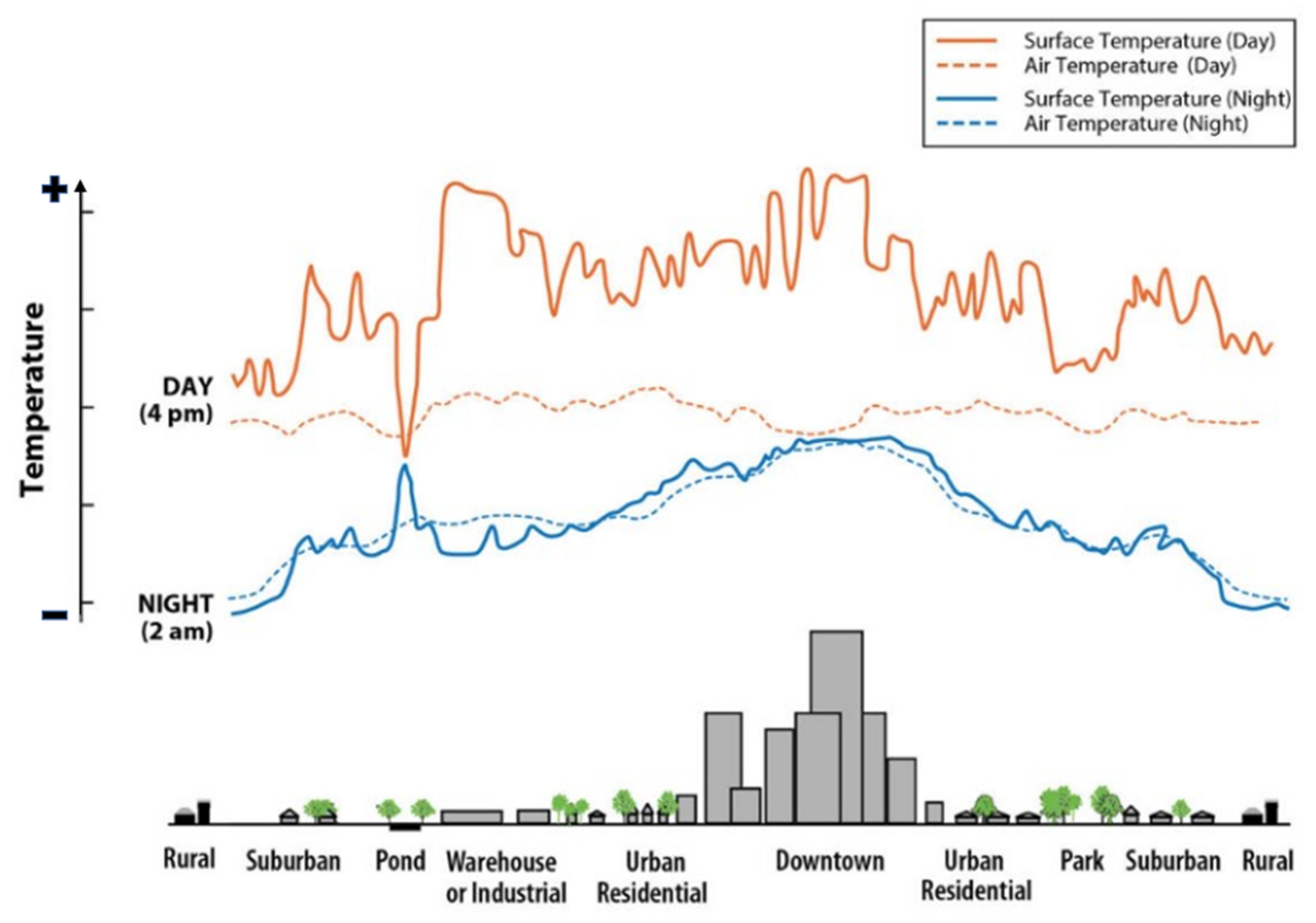
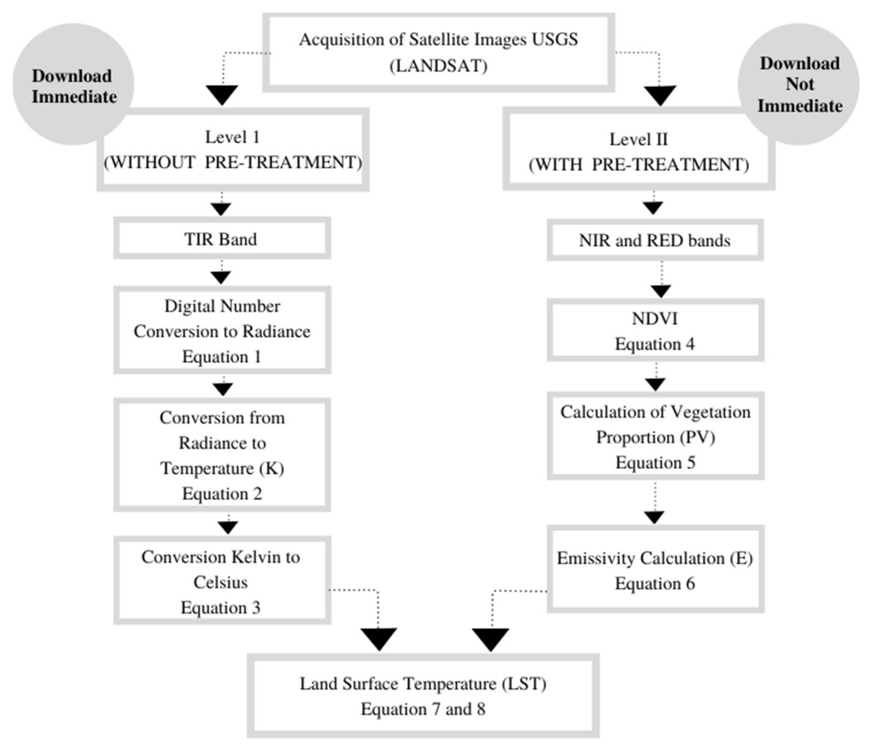
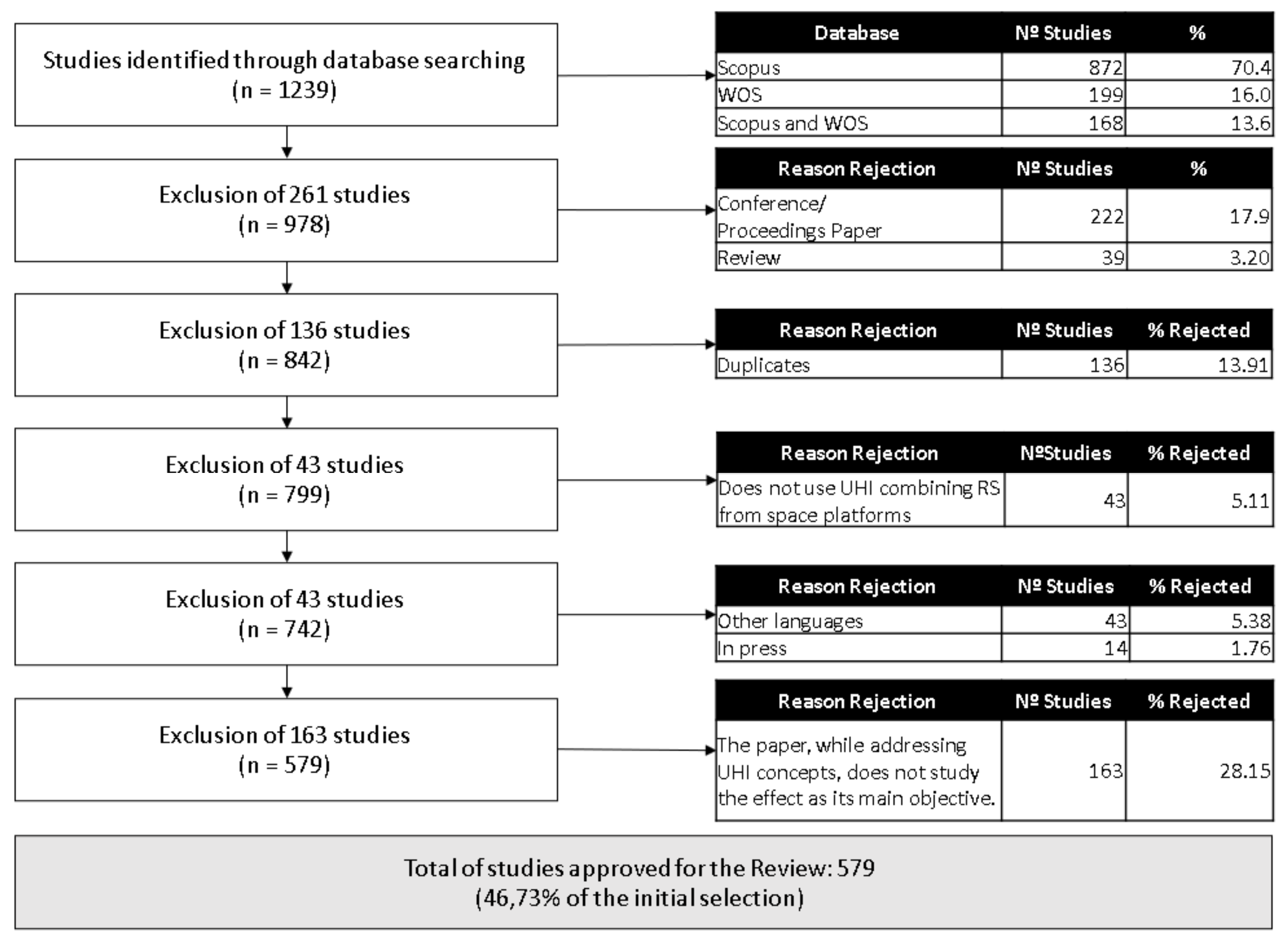
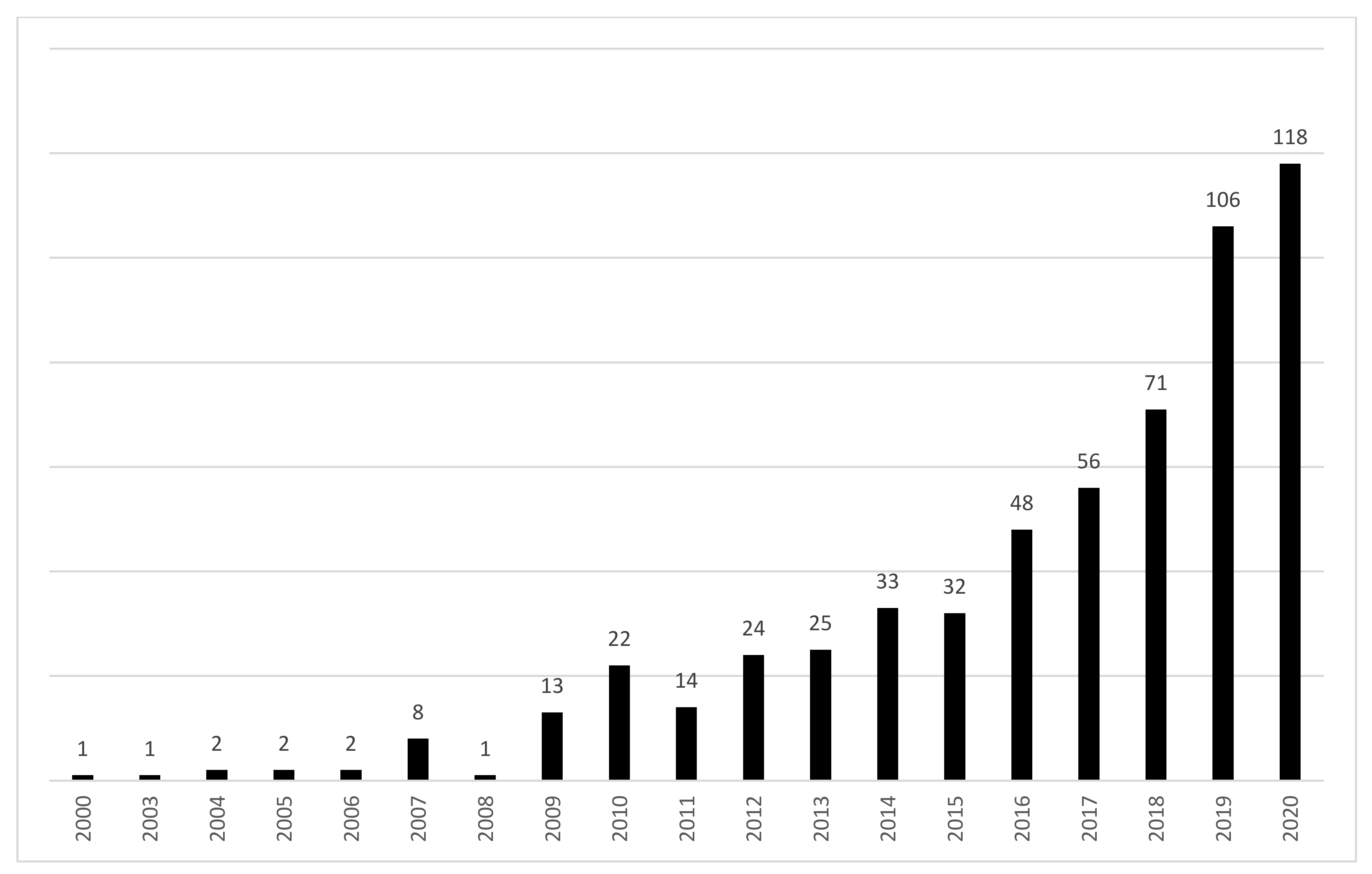
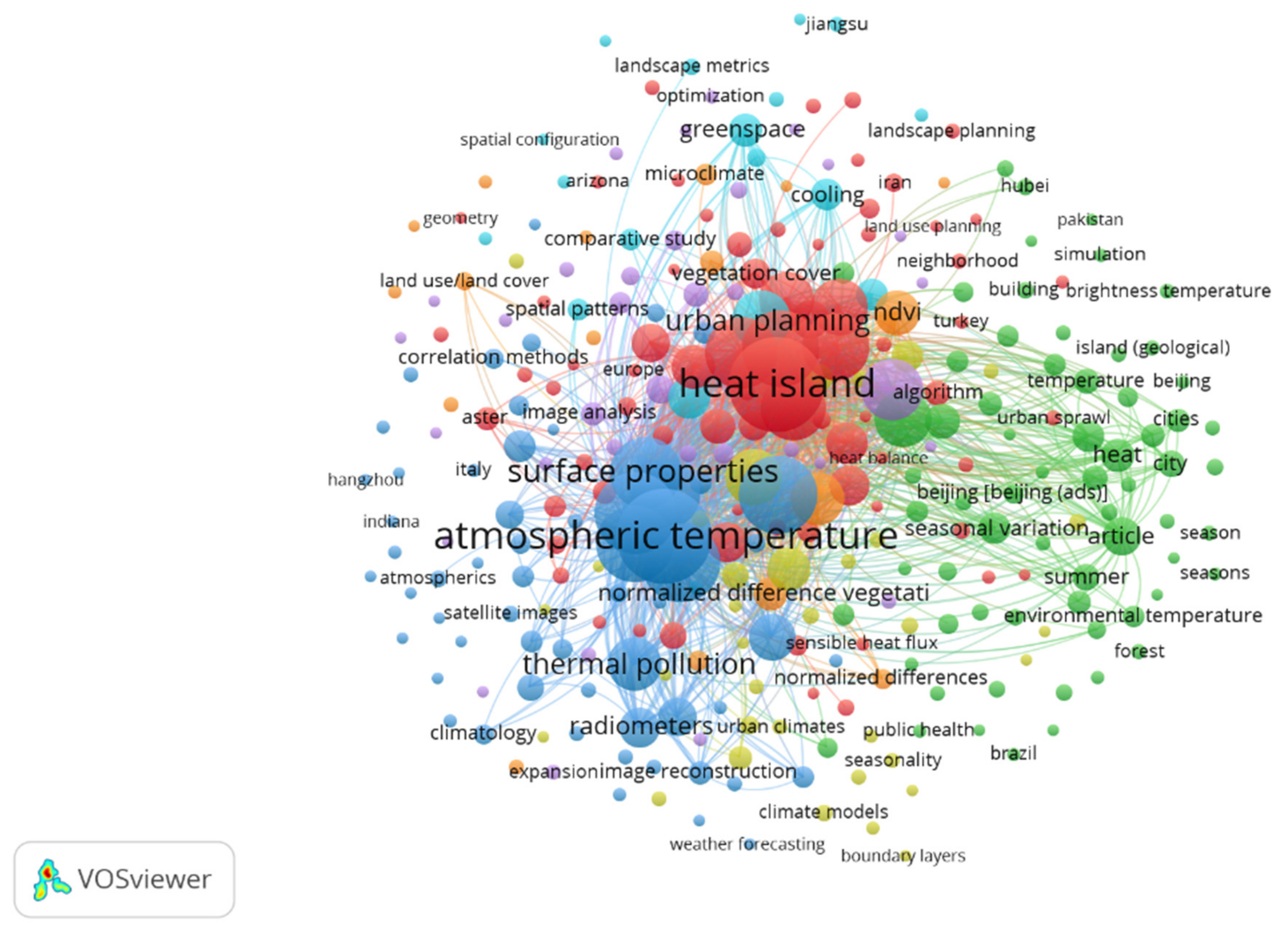
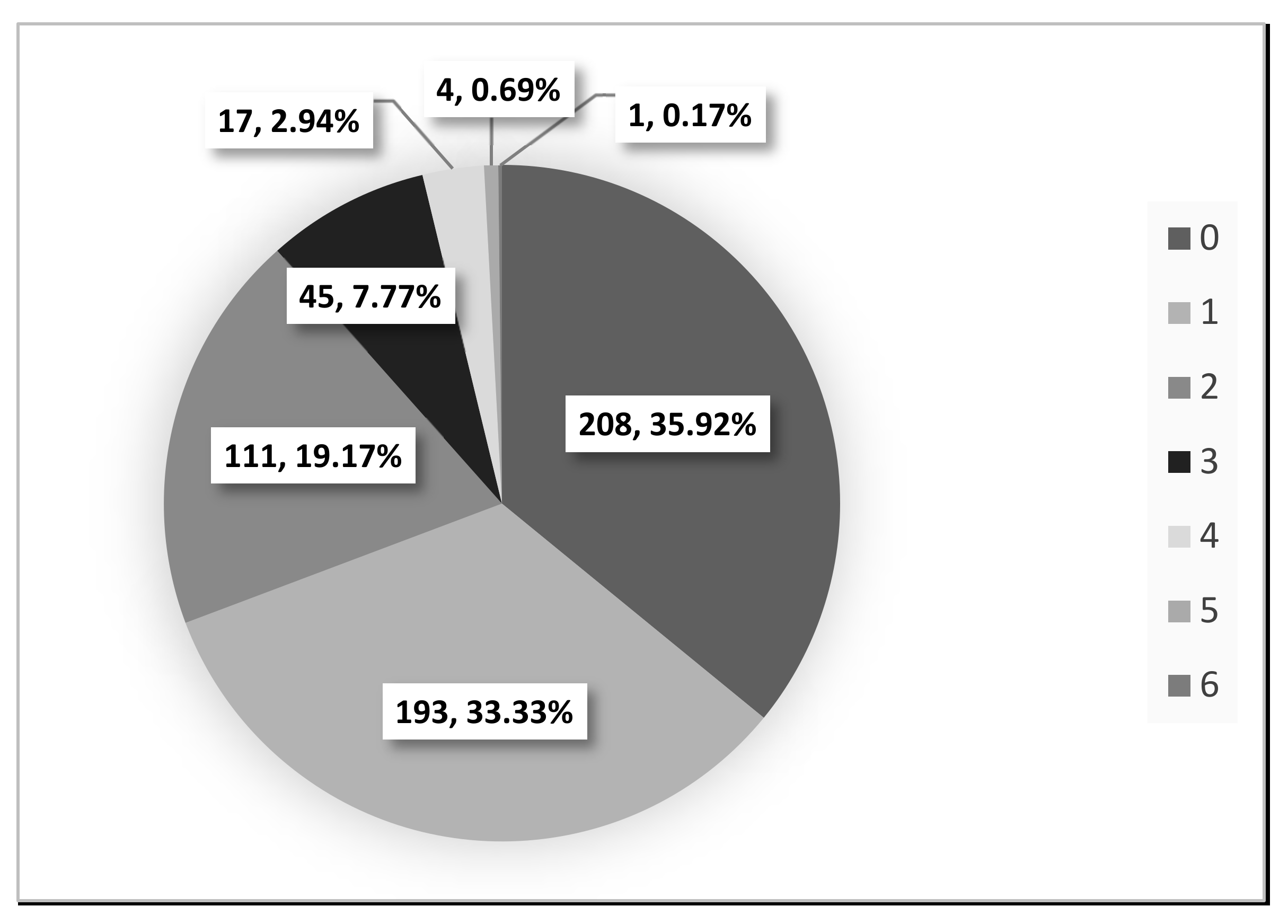
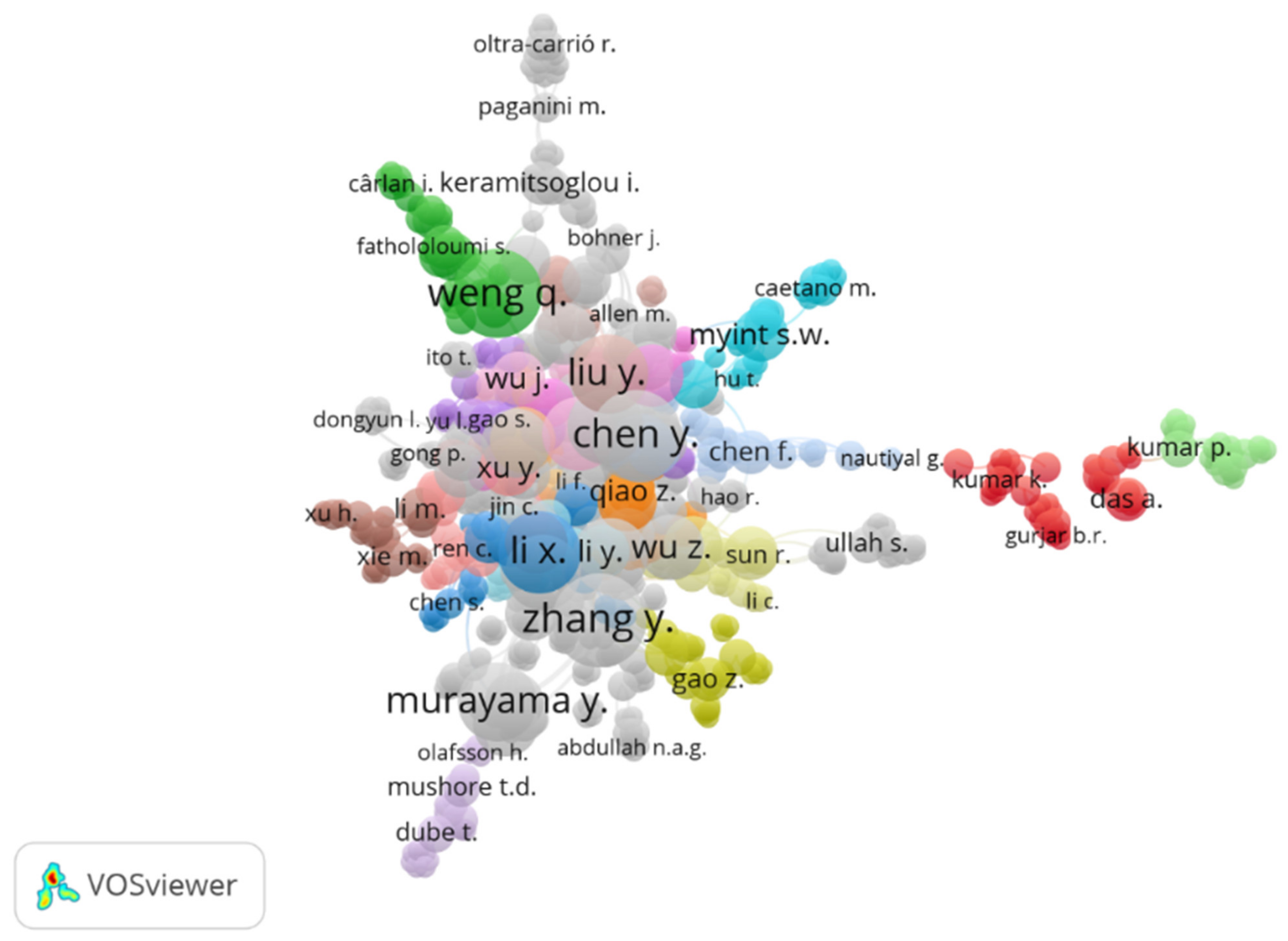
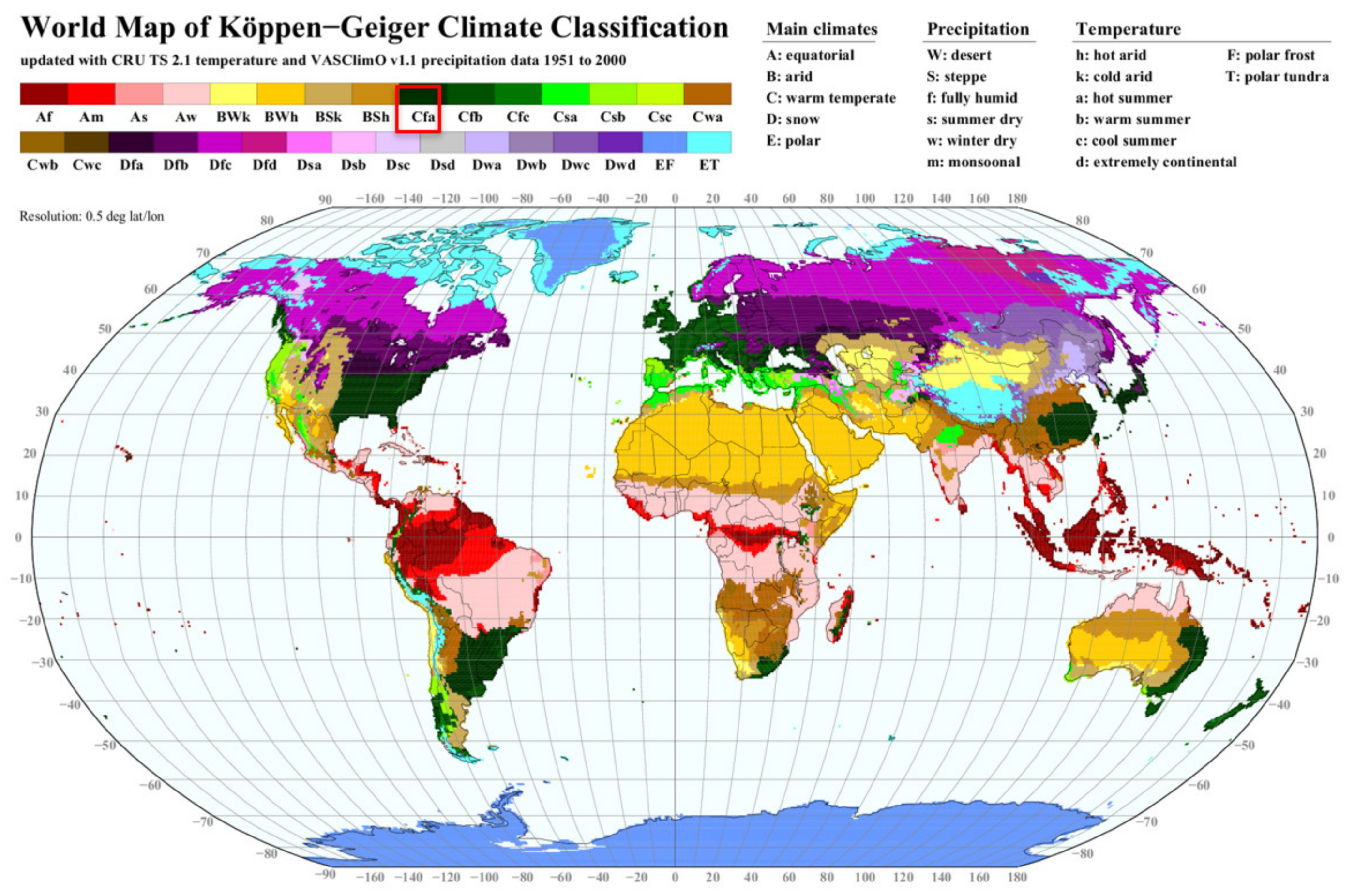
Table 1.
Summary of the thermal sensors most commonly applied in UHI studies (adapted from [37,41]).
| Sensor | Satellite Platform | Orbital Frequency | Spatial Resolution | Spectral Bands (µm) | Number Band | Data Available Since |
|---|---|---|---|---|---|---|
| AATSR | Envisat | 35 days | 1 km (approx.) | 11 and 12 | TIR | 2002–2012 |
| ASTER | Terra | Twice daily | 90 m | 8.125–8.475 8.475–8.825 8.925–9.275 10.25–10.95 10.95–11.65 | 10 11 12 13 14 | 1999 |
| AVHRR (Advanced Very High Resolution Radiometer) | NOAA 6, 8 10, TIROS-N | Twice daily | 1.1 km (approx.) | 10.3–11.3 11.5–12.5 | 4 5 | 1978–2001 |
| AVHRR/2 (Advanced Very High Resolution Radiometer/2) | NOAA 7, 9, 11, 12, 13, 14 | Twice daily | 1.1 km (approx.) | 10.3–11.3 11.5–12.5 | 4 5 | 1981–2007 |
| AVHRR/3 (Advanced Very High Resolution Radiometer) | METOP-A, B, C | 29 days | 1.1 km (approx.) | 10.3–11.3 11.5–12.5 | 4 5 | 2006 |
| AVHRR/3 (Advanced Very High Resolution Radiometer/3) | NOAA 15, 16, 17, 18, 19 | Twice daily | 1.1 km (approx.) | 10.3–11.3 11.5–12.5 | 4 5 | 1998 |
| ETM+ | Landsat 7 | 16 days | Collected at 60 m and resampled to 30 m | 10.4–12.5 | 6 | 1999 |
| GOES Imager | GOES | Geostationary | 4 km (approx.) | 10.2–11.2 11.5–12.5 | TIR | 1974 |
| IRMSS (Infrared Multispectral Scanner) | HJ-1B | 31 days | 300 m | 10.5–12.5 | TIR | 2008–2018 |
| IRMSS (Infrared Multispectral Scanner) | CBERS 1 | 26 days | 160 m | 10.4–12.5 | 4 | 1999–2003 |
| IRMSS (Infrared Multispectral Scanner) | CBERS 2 | 26 days | 160 m | 10.4–12.5 | 4 | 2003–2009 |
| IRMSS (Infrared Multispectral Scanner) | CBERS 2B | 26 days | 160 m | 10.4–12.5 | 4 | 2007–2010 |
| IRMSS-2 (HJ) (Infrared Multispectral Scanner-2) | HJ-2A and HJ-2B | 4 days | 300 m | 10.5–12.5 | TIR | 2020 |
| IRS (Infrared Medium Resolution Scanner) | CBERS 4 | 26 days | 80 m | 10.4–12.5 | 12 | 2014 |
| IRS (Infrared Medium Resolution Scanner) | CBERS 4A | 31 days | 80 m | 10.4–12.5 | 12 | 2019 |
| MODIS | Terra | Twice daily | 1 km (approx.) | 10.78–11.28 11.77–12.27 | 31 32 | 1999 |
| MODIS | Aqua | Twice daily | 1 km (approx.) | 10.78–11.28 11.77–12.27 | 31 32 | 2002 |
| SEVIRI | Meteosat-8 | Geostationary | 3 km (approx.) | 10.812 | TIR | 2005 |
| TIRS | Landsat 8 | 16 days | Collected at 100 m and resampled to 30 m | 10.6–11.2 11.5–12.5 | 10 11 | 2013 |
| TIRS 2 | Landsat 9 | 16 days | Collected at 100 m and resampled to 30 m | Similar TIRS | Similar TIRS | Launch planned for 09/23/2021 |
| TM | Landsat 4 | 16 days | Collected at 120 m and resampled to 30 m | 10.4–12.5 | 6 | 1982–1993 |
| TM | Landsat 5 | 16 days | Collected at 120 m and resampled to 30 m | 10.4–12.5 | 6 | 1984–2011 |
Table 2.
Published papers by continent/sub-continent.
| Continent | No. of Publications | % of Publications |
|---|---|---|
| Asia | 405 | 69.94 |
| Europe | 65 | 11.23 |
| North America | 59 | 10.19 |
| Africa | 18 | 3.11 |
| South America | 12 | 2.07 |
| Australian Area | 4 | 0.69 |
| Antarctic Area | 2 | 0.35 |
| Studies Involving More than One Continent/Sub-Continent | ||
| Africa and Europe | 1 | 0.17 |
| Asia and Europe | 7 | 1.21 |
| Asia and North America | 3 | 0.52 |
| More than two continents | 3 | 0.52 |
| Total | 579 | 100 |
Table 3.
Climatic zone of study areas.
| Group | Climate | Acronym/Name | No. of Publications That Mentioned the Climate |
|---|---|---|---|
| C | Temperate | Cfa—Humid Subtropical Climate | 188 |
| D | Continental | Dwa—Monsoon-Influenced Hot-Summer Humid Continental Climate | 81 |
| C | Temperate | Cwa—Monsoon-Influenced Humid Subtropical Climate | 54 |
| A | Tropical | Aw—Tropical Savanna Climate | 50 |
| C | Temperate | Cfb—Temperate Oceanic Climate | 42 |
| B | Dry | BWh—Hot Desert Climate | 37 |
| B | Dry | BSk—Cold Semi-Arid Climate | 33 |
| C | Temperate | Csa—Hot-Summer Mediterranean Climate | 31 |
| B | Dry | BSh—Hot Semi-Arid Climate | 22 |
| A | Tropical | Af—Tropical Rainforest Climate | 15 |
| D | Continental | Dfb—Warm-Summer Humid Continental Climate | 13 |
| A | Tropical | Am—Tropical Monsoon Climate | 11 |
| C | Temperate | Cwb—Subtropical Highland Climate | 6 |
| D | Continental | Dfa—Hot-Summer Humid Continental Climate | 6 |
| D | Continental | Dfc—Subarctic Climate | 4 |
| C | Temperate | Csb—Warm-Summer Mediterranean | 3 |
| B | Dry | BWk—Cold Desert Climate | 2 |
| D | Continental | Dwb—Monsoon-Influenced Warm-Summer Humid Continental Climate | 1 |
| E | Polar | ET—Tundra | 1 |
Table 4.
Top 15 most frequently cited keywords.
| Keyword | No. of Citation |
|---|---|
| land surface temperature | 285 |
| urban heat island | 285 |
| heat island | 282 |
| atmospheric temperature | 279 |
| remote sensing | 211 |
| surface temperature | 196 |
| landforms | 188 |
| land surface | 171 |
| surface properties | 164 |
| surface measurement | 149 |
| China | 141 |
| satellite imagery | 140 |
| urbanization | 134 |
| land use | 111 |
| urban planning | 110 |
Table 5.
Study of the UHI effect.
| Study Approach | Main Data Used | No. of Papers | % |
|---|---|---|---|
| Rural versus urban areas and Seasonality | Including papers that used extra data (weather network, LULC, building construction, LCZs, on-site measurement) | 416 | 71.85 |
| Environmental | Environmental Data Vegetation, biophysical, biochemical, water body, and wetland data | 61 | 10.53 |
| Models (IVs, mathematical, computational) | Satellite data; extra data (weather network, LULC, building construction, LCZs, on-site measurement, historical data) | 31 | 5.35 |
| Health and Social | Census, health data, questionnaire application | 28 | 4.84 |
| Specific areas of study | Complementary data to identify local specificities (as petrochemical, arid zones, and mountainous areas) | 21 | 3.63 |
| Air pollution, energy consumption, and economic factors | Consumption and pollutant data | 15 | 2.60 |
| Focus on Predictability | Historical data | 7 | 1.20 |
| Total | 579 | 100 |
Table 6.
Most used satellites/sensors to obtain LST data.
| Satellite | Exclusive Use | Combination | ||
|---|---|---|---|---|
| No. of Papers | % | No. of Papers | % | |
| Landsat | 317 | 54.75 | 396 | 68.39 |
| MODIS | 103 | 17.79 | 185 | 31.95 |
| ASTER | 15 | 2.59 | 36 | 6.22 |
| NOAA/AVHRR | 1 | 0.17 | 7 | 1.21 |
| METEOSAT | - | - | 3 | 0.52 |
Table 7.
Most used satellites sensors in the LULC estimation.
| Satellite | Exclusive Use | Combination | ||
|---|---|---|---|---|
| No. of Papers | % | No. of Papers | % | |
| Landsat | 211 | 36.44 | 324 | 55.96 |
| MODIS | 51 | 8.81 | 95 | 16.41 |
| ASTER | 11 | 1.90 | 32 | 5.53 |
| IKONOS | 5 | 0.86 | 21 | 3.63 |
| SPOT | 9 | 1.55 | 14 | 2.42 |
Table 8.
Six most used software programs.
| Keyword | Key Applications in Papers | Exclusive Use | Combination | ||
|---|---|---|---|---|---|
| No. of Papers | % | No. of Papers | % | ||
| ArcGIS | Spatial image analysis and processing | 60 | 10.36 | 178 | 30.74 |
| ENVI | 28 | 4.84 | 93 | 16.06 | |
| Google Earth | 3D representation of the earth based mainly on satellite imagery used to identify LULC classes | 30 | 5.18 | 71 | 12.26 |
| ERDAS Image | Spatial image analysis and processing | 11 | 1.90 | 43 | 7.43 |
| FRAGSTATS | Calculating landscape metrics | - | - | 39 | 6.74 |
| SPSS | Statistical calculations | - | - | 33 | 5.70 |
Table 9.
Ten indices/indicators most used.
| Index | No. of Citation |
|---|---|
| NDVI | 190 |
| Enhanced Vegetation Index (EVI); Fraction Vegetation Cover (FVC); Photosynthesis | 105 |
| Built-up | 78 |
| LULC and Bareness | 73 |
| NDBI | 71 |
| Percent of Impermeable Surface (%ISA)/Impervious Surface Areas (ISA) | 68 |
| Dimension, Altitude, Latitude, Digital Elevation Model (DEM) | 42 |
| Demographic/Social Data | 33 |
| Water Bodies | 31 |
| Albedo | 26 |
Table 10.
Papers by the number of statistical techniques applied.
| No. of Statistical Techniques Applied | No. of Papers | % |
|---|---|---|
| 0 | 36 | 6.22 |
| 1 | 232 | 40.07 |
| 2 | 195 | 33.68 |
| 3 | 62 | 10.71 |
| 4 | 30 | 5.18 |
| 5 | 14 | 2.42 |
| 6 | 8 | 1.38 |
| Total | 579 | 100 |
Table 11.
Papers by statistical technique.
| No. of Statistical Techniques Applied | No. of Papers | % |
|---|---|---|
| Correlation | 224 | 38.69 |
| Regression | 210 | 36.27 |
| Descriptive Statistics | 128 | 22.11 |
| Others | 60 | 10.36 |
| Machine Learning | 27 | 4.66 |
| Model/Method | 27 | 4.66 |
| Dispersion | 25 | 4.32 |
| Tests | 20 | 3.45 |
| Variance | 12 | 2.07 |
| Spatial Statistics | 3 | 0.52 |
Table 12.
Main findings of the studies.
| Main Conclusions | No. of Papers | % |
|---|---|---|
| UHI identified at a study site | 579 | 100 |
| Recommendations for mitigating measures considering civil construction, vegetation, and maintenance of water bodies | 229 | 39.55 |
| Seasonality influences the results (different times of the day and/or seasons) | 71 | 12.26 |
| The methods and models tested for the study of UHI were efficient | 49 | 8.46 |
| The morphology, density, and choice of vegetation was appropriate to the specificity of the site and enhances the mitigation effects | 38 | 6.56 |
| Recommendations on socioenvironmental, economic, and health measures to mitigate the effects of UHI | 15 | 2.59 |
| Association of the UHI with atmospheric contamination and wind circulation, with recommendations for mitigating measures | 11 | 1.90 |
| Association of the UHI with flooding and rainfall | 8 | 1.39 |
Table 13.
Highlight of some reasons for UHI and SUSHI´s formation.
| Factors | |
|---|---|
| Civil Constructions | Topographical features, building standards, building cooling, landscape configuration, urban morphology, spatial patterns of land use and occupancy [106,107,108], texture and spatial distribution [109], rural/urban areas with low vegetation density, in bare soil [110,111,112,113]. |
| Three-dimensional urban design (such as height, volume, and surface area of the buildings, and the footprint and shadow volume) showed greater influence relative to two-dimensional ones (such as building rooftop area, street, and vegetation) [114]. | |
| Heterogeneity in the composition of built surfaces and areas [115]. | |
| Hydrological and soil permeability interference [116]. | |
| Urban Size | Influence on surface heat flux, soil/air temperature, humidity, and wind circulation, resulting in differences in urban–rural energy balance [117]. |
| Heat Emission | Night lights [118,119], heat emission from industrial and transportation sources [120,121,122]. |
| Environment | Wind [123], wind speed, and land surface conditions, especially in the morning, corroborate the advance of warm air [124], aerosols can influence/limit diurnal surface heating in dry seasons [125]. |
Table 14.
Indicators for understanding UHI and SUHI.
| Indicator | |
|---|---|
| IV | NDVI, NDBI [126], PV (that can show better results in the regressions applied when compared to NDVI) [127], landscape effects (that may have more impact than socioenvironmental data) [89]. |
| Construction and soil | Characteristics and types of soils, LULC [128,129], imperviousness [130], albedo-exposed land areas [131], presence of surface contaminants, as hydrocarbons used in bioremediation processes, whose soils can present higher thermal signatures when revegetated [132]. |
| Social, economic, and health | Population size [1], especially in cities with continental climate [133], economics, social, environmental, population health, anthropogenic heat flux [134,135,136,137,138,139,140,141,142,143,144], and in specific events/actions [91,145]. |
Table 15.
Main consequences of the UHI and SUHI effect.
| Main Consequences | |
|---|---|
| Environment | Atmospheric instability [167] that can influence the dispersion of pollutants [83], thermal circulations [168], convective precipitation [135,169], urban flooding [136]. |
| Social and health | Biological risks [170], as the increase in mortality and heath [134,144], heat stress-related diseases (especially at night) [143], such as cardiovascular, respiratory, circulatory, emotional disorders [171], anxiety, sleep problems, and depression [142]. |
| Economic | Regulation of the values practiced in the real estate market, whose properties most affected by the effect are cheaper [138], and preference in housing green areas and open spaces by high-income and educated families [88], which suggests understanding and studies regarding social vulnerability associated with residential segregation [172]. |
| Increased electricity consumption in summer (due to the need for cooling/use of air conditioning), and minimized in winter (where the need for heating was not so necessary) [173], especially in areas inhabited by the high-income population, which have the means to regulate temperature, promoting thermal comfort [140]. It is noteworthy that the use of air conditioning can corroborate the increase of primary pollutant emissions and ozone generation [174], and increases the financial costs [175]. |
Table 16.
Mitigation of the UHI and SUHI effect.
| Mitigation | |
|---|---|
| Construction and LULC | Conversion of vacant land into green areas to minimize the effects of thermal discomfort [139], knowledge of local parameters, urban plantation, decentralization of urban areas [176,177,178,179], minimizing impervious areas and bare soils (such as abandoned land) [176], and diversification and balance of LULC elements, combining urban and vegetated areas, optimizing spatial configuration [178]; industrial relocation, buildings demolition, and brownfield redevelopment [180]; optimization of green land cover configuration [181] (in relatively small cities) or controlling sprawl (in larger cities) reducing the ratio of compaction in urban sprawl [182]; keeping the balance between urban and non-urban uses [183]; light-colored skyscrapers with glass curtain walls systems (which showed relatively low LST) [184]. |
| Environmental | Preservation of water bodies [80,174,185,186] with simple geometry. The area of the waterbody is also a factor that influences temperature variation and, with high surface moisture, are less efficient than a water body (such as a river) [187] but can attenuate surface temperature better than vegetation cover, especially in dry seasons [188]. Increased proportion of vegetation at the expense of impermeable areas [189,190], distribution of trees and taking advantage of their shade effects [191], green surfaces/roofs [192,193,194,195,196,197,198,199,200]. The relationship between the presence of vegetation and cooling is not linear [201], and additional studies are needed to evaluate local specificities and needs. There are cases, for example, that associate the use of large trees with negative effects on nighttime cooling [202], due to higher heat retention as a consequence of a lower SVF [203]. Therefore, their characteristics must be evaluated to identify the most suitable and favorable vegetal species, arrangements, and strategies for heat exchange in a region. In addition to increasing the volume of vegetation areas at a site [204], evaluating the spatial pattern, shape, canopy cover [205], leaf density, and area of influence of heat regulation/shade effects [206,207,208]. Large parks did not present advantages over small ones [209]. |
| Social, economic, and health | Encouraging the use of public transportation to reduce the circulation of cars and the emission of atmospheric pollutants [137]. Development of social measures, such as subsidies for electricity [173], and creation of heat warning and health surveillance systems, which alert users to the occurrence of heat waves [141]. |
Table 17.
Eight most recurrent bibliographic references in the studies.
| Reference | No. of Papers | % |
|---|---|---|
| J. A. Voogt and T. R. Oke, “Thermal remote sensing of urban climates,” Remote Sens. Environ., vol. 86, no. 3, pp. 370–384, 2003, doi: 10.1016/S0034-4257(03)00079-8 [12]. | 105 | 18.13 |
| F. Yuan and M. E. Bauer, “Comparison of impervious surface area and normalized difference vegetation index as indicators of surface urban heat island effects in Landsat imagery,” Remote Sens. Environ., vol. 106, no. 3, pp. 375–386, Feb. 2007, doi: 10.1016/j.rse.2006.09.003 [210]. | 42 | 7.25 |
| M. L. Imhoff, P. Zhang, R. E. Wolfe, and L. Bounoua, “Remote sensing of the urban heat island effect across biomes in the continental USA,” Remote Sens. Environ., vol. 114, no. 3, pp. 504–513, 2010, doi: 10.1016/j.rse.2009.10.008.n [2]. | 30 | 5.18 |
| Q. Weng, D. Lu, and J. Schubring, “Estimation of land surface temperature-vegetation abundance relationship for urban heat island studies,” Remote Sens. Environ., vol. 89, no. 4, pp. 467–483, 2004, doi: 10.1016/j.rse.2003.11.005 [23]. | 30 | 5.18 |
| A. J. Arnfield, “Two decades of urban climate research: a review of turbulence, exchanges of energy and water, and the urban heat island,” Int. J. Climatol., vol. 23, no. 1, pp. 1–26, Jan. 2003, doi: 10.1002/joc.859 [8]. | 28 | 4.84 |
| T. R. Oke, “The energetic basis of the urban heat island (Symons Memorial Lecture, 20 May 1980).,” Q. Journal, R. Meteorol. Soc., vol. 108, no. 455, pp. 1–24, 1982, doi:10.1002/qj.49710845502 [1]. | 28 | 4.84 |
| J. A. Sobrino, J. C. Jiménez-Muñoz, and L. Paolini, “Land surface temperature retrieval from LANDSAT TM 5,” Remote Sens. Environ., vol. 90, no. 4, pp. 434–440, Apr. 2004, doi: 10.1016/j.rse.2004.02.003 [53]. | 26 | 4.49 |
| X.-L. Chen, H.-M. Zhao, P.-X. Li, and Z.-Y. Yin, “Remote sensing image-based analysis of the relationship between urban heat island and land use/cover changes,” Remote Sens. Environ., vol. 104, no. 2, pp. 133–146, Sep. 2006, doi: 10.1016/j.rse.2005.11.016 [211]. | 25 | 4.32 |
Table 18.
Number of publications by author.
| No. of Publications Associated with the Author’s Name | No. of Authors | % of Authors |
|---|---|---|
| 1 | 1136 | 77.02 |
| 2 | 181 | 12.27 |
| 3 | 78 | 5.29 |
| 4 | 27 | 1.83 |
| 5 | 17 | 1.15 |
| 6 | 12 | 0.81 |
| 7 | 4 | 0.27 |
| 8 | 5 | 0.34 |
| 9 | 3 | 0.20 |
| 10 | 2 | 0.14 |
| >10 | 10 | 0.68 |
| Total | 1475 | 100 |
Table 19.
Ten most cited papers.
| Paper | No. of Citations |
|---|---|
| X.-L. Chen, H.-M. Zhao, P.-X. Li, and Z.-Y. Yin, “Remote sensing image-based analysis of the relationship between urban heat island and land use/cover changes,” Remote Sens. Environ., vol. 104, no. 2, pp. 133–146, Sep. 2006, doi: 10.1016/j.rse.2005.11.016. [211] | 849 |
| M. L. Imhoff, P. Zhang, R. E. Wolfe, and L. Bounoua, “Remote sensing of the urban heat island effect across biomes in the continental USA,” Remote Sens. Environ., vol. 114, no. 3, pp. 504–513, 2010, doi: 10.1016/j.rse.2009.10.008. [2] | 648 |
| J. Li, C. Song, L. Cao, F. Zhu, X. Meng, and J. Wu, “Impacts of landscape structure on surface urban heat islands: A case study of Shanghai, China,” Remote Sens. Environ., vol. 115, no. 12, pp. 3249–3263, Dec. 2011, doi: 10.1016/j.rse.2011.07.008. [212] | 499 |
| W. Zhou, G. Huang, and M. L. Cadenasso, “Does spatial configuration matter? Understanding the effects of land cover pattern on land surface temperature in urban landscapes,” Landsc. Urban Plan., vol. 102, no. 1, pp. 54–63, 2011, doi: 10.1016/j.landurbplan.2011.03.009. [213] | 418 |
| A. Buyantuyev and J. Wu, “Urban heat islands and landscape heterogeneity: Linking spatiotemporal variations in surface temperatures to land-cover and socioeconomic patterns,” Landsc. Ecol., vol. 25, no. 1, pp. 17–33, 2010, doi: 10.1007/s10980-009-9402-4. [156] | 416 |
| X. Cao, A. Onishi, J. Chen, and H. Imura, “Quantifying the cool island intensity of urban parks using ASTER and IKONOS data,” Landsc. Urban Plan., vol. 96, no. 4, pp. 224–231, Jun. 2010, doi: 10.1016/j.landurbplan.2010.03.008. [214] | 266 |
| J. P. Connors, C. S. Galletti, and W. T. L. Chow, “Landscape configuration and urban heat island effects: Assessing the relationship between landscape characteristics and land surface temperature in Phoenix, Arizona,” Landsc. Ecol., vol. 28, no. 2, pp. 271–283, 2013, doi: 10.1007/s10980-012-9833-1. [107] | 257 |
| R. Amiri, Q. Weng, A. Alimohammadi, and S. K. Alavipanah, “Spatial-temporal dynamics of land surface temperature in relation to fractional vegetation cover and land use/cover in the Tabriz urban area, Iran,” Remote Sens. Environ., vol. 113, no. 12, pp. 2606–2617, Dec. 2009, doi: 10.1016/j.rse.2009.07.021. [215] | 235 |
| Q. Weng, “Fractal analysis of satellite-detected urban heat island effect,” Photogramm. Eng. Remote Sensing, vol. 69, no. 5, pp. 555–566, 2003, doi: 10.14358/PERS.69.5.555. [109] | 204 |
| N. Schwarz, S. Lautenbach, and R. Seppelt, “Exploring indicators for quantifying surface urban heat islands of European cities with MODIS land surface temperatures,” Remote Sens. Environ., vol. 115, no. 12, pp. 3175–3186, Dec. 2011, doi: 10.1016/j.rse.2011.07.003. [216] | 199 |
Table 20.
Number of citations per paper (data analyzed by consulting the database on 15 March 2021).
Table 20.
Number of citations per paper (data analyzed by consulting the database on 15 March 2021).
| Citation | No. of Papers | % |
|---|---|---|
| 0 | 48 | 8.29 |
| 1–3 | 97 | 16.75 |
| 4–6 | 63 | 10.88 |
| 7–10 | 55 | 9.50 |
| 11–18 | 85 | 14.68 |
| 19–25 | 45 | 7.77 |
| 26–40 | 66 | 11.40 |
| 41–60 | 38 | 6.56 |
| 61–80 | 33 | 5.70 |
| 81–100 | 10 | 1.73 |
| 101–125 | 9 | 1.55 |
| 126–160 | 13 | 2.25 |
| 161–250 | 10 | 1.73 |
| 251–500 | 5 | 0.86 |
| 501–849] | 2 | 0.35 |
| Total | 579 | 100 |
Publisher’s Note: MDPI stays neutral with regard to jurisdictional claims in published maps and institutional affiliations. |
© 2021 by the authors. Licensee MDPI, Basel, Switzerland. This article is an open access article distributed under the terms and conditions of the Creative Commons Attribution (CC BY) license (https://creativecommons.org/licenses/by/4.0/).
Share and Cite
MDPI and ACS Style
Almeida, C.R.d.; Teodoro, A.C.; Gonçalves, A. Study of the Urban Heat Island (UHI) Using Remote Sensing Data/Techniques: A Systematic Review. Environments 2021, 8, 105. https://0-doi-org.brum.beds.ac.uk/10.3390/environments8100105
AMA Style
Almeida CRd, Teodoro AC, Gonçalves A. Study of the Urban Heat Island (UHI) Using Remote Sensing Data/Techniques: A Systematic Review. Environments. 2021; 8(10):105. https://0-doi-org.brum.beds.ac.uk/10.3390/environments8100105
Chicago/Turabian StyleAlmeida, Cátia Rodrigues de, Ana Cláudia Teodoro, and Artur Gonçalves. 2021. "Study of the Urban Heat Island (UHI) Using Remote Sensing Data/Techniques: A Systematic Review" Environments 8, no. 10: 105. https://0-doi-org.brum.beds.ac.uk/10.3390/environments8100105
Note that from the first issue of 2016, this journal uses article numbers instead of page numbers. See further details here.