Potential Influence of Sewage Phosphorus and Wet and Dry Deposition Detected in Fish Collected in the Athabasca River North of Fort McMurray

Abstract

The health of fish is a primary indicator of ecosystem response in the Oil Sands Region of northeastern Alberta. However, industrial activity is accompanied by other stressors, such as the discharge of sewage, municipal activity, forest fires, and natural weathering and erosion of bitumen. To combat the spatial confounding influences, we examined white sucker (Catostomus commersonii) captured in the Athabasca River at sites over time (2011–2019) and included covariates to account for the possible sources of influence. The analyses suggest spatially heterogeneous influences of natural factors on fish, such as discharge and air temperature, but also the influence of sewage phosphorus and precipitation. Among the stressors examined here, precipitation may be the most complex and may include a mixture of sources including inputs from tributaries, urban activity, industrial development, and forest fires. Although suggestive, the attribution of variance and detection of changes are affected by sample sizes in some years; these analyses may have missed effects or misspecified important relationships, especially in males. Despite these limitations, the analyses suggest potential differences may be associated with precipitation and highlight the need to integrate robust information on known and suspected stressors in future monitoring of aquatic ecosystems in the oil sands region and beyond.

1. Introduction

Bitumen deposits in the Oil Sands Region (OSR) of northeastern Alberta are the third-largest known reserves of hydrocarbons in the world. The bitumen underlies 142,000 km² of surface area and is separated into the Cold Lake, Peace, and Athabasca administrative sub-regions. The deposits are accompanied by expansive industrial extraction and processing of bitumen through surface mining and in situ techniques. Oil sands development is the predominant human activity in the region and is associated with concerns of undocumented environmental effects and the potential for long-term harm [1,2].

Extensive effort has been expended in the last decade to address these concerns and determine the cumulative influence of oil sands industrial activity (OSIA) in the OSR. Much has been learned, including the potential contribution of contaminants of concern (CoCs) from surface mines [3,4,5,6,7] and in situ facilities [8,9] to the ambient environment. However, the OSR is a complex environment with many overlapping anthropogenic and natural stressors [1,2,10]. More specifically, research has clearly shown the influence of OSIA, but the accompanying, overlapping, and potentially interfering effects of other local, regional, and global stressors have also been identified [11,12,13,14,15,16,17,18,19,20,21,22,23,24,25].

Disentangling the influence of multiple stressors on aquatic biota residing in flowing waters has been especially challenging in the OSR. In streams, CoCs are often found at elevated concentrations at sites adjacent to oil sands facilities [11,14,26,27,28], and aquatic indicators captured at these locations, such as fish also often show effects consistent with exposure to these compounds [28,29]. However, CoCs can derive directly and indirectly from both natural and industrial sources [11,12,26,30,31]. Materials originating from OSIA can be released to the atmosphere which may deposit to water bodies or the landscape, can be discharged via effluents, or, while rare, seep from tailings ponds [32,33,34]. Local industrial development can also affect the hydrology of watersheds exacerbating or otherwise altering exposure regimes [30,35]. Natural and non-OSIA sources are also present and include forest fires [36,37], urban activity [38], weathering and erosion of bitumen outcrops [33,39], accumulation of sediments in depositional areas [39], and discharge of groundwater naturally in contact with bitumen [21]. Additionally, the health of fish in reference areas and within the OSR varies annually [33,40] suggesting the potential influence of other natural stressors, such as temperature and river discharge on biotic indicators [41,42,43]. Consequently, discerning the role of OSIA on any detected changes in biota residing in the OSR can be difficult [44].

A primary component of regional monitoring in the OSR is the analysis of fish health in the mainstem Athabasca River. Evidence of change has been observed in white sucker (Catostomus commersonii) collected near oil sands facilities relative to upstream reference areas [33,40,45]. While influences have been hypothesized, several confounding stresses are present. Along with the stressors already described, such as the natural erosion of bitumen, the potentially overlapping influences in the Athabasca River also include discharge of sewage from the Fort McMurray wastewater treatment plant (FMM WWTP) [33,40,45,46] and the delivery of CoCs from upstream areas [47]. The existing literature and the occurrence of multiple stressors possibly affecting fish in the OSR suggest approaches to partition variability into potential sources are needed to identify and isolate the effects of industrial development and focus future monitoring efforts [48,49].

Here we build on previous research examining the health of white sucker collected in the Athabasca River from 2011 to 2013 [33] using additional data collected in 2014, 2016, and 2019. Using this 6-year data set collected over a decade, we used a site-specific approach (e.g., [48]) to address potential upstream-downstream confounding influences in the Athabasca River and asked two related questions. First, we determined if variation within the fish data set could be attributed to known and suspected sources of variation at each focal study location. These analyses first included temperature and river discharge, but the potential influence of sewage phosphorus and local precipitation was also evaluated in an exploratory analysis. Second, we determined if potentially relevant differences could be attributed to these factors or if large residual variation suggested additional factors may be affecting the health of fish. These analyses, while affected by low sample sizes in later years (2014–2019), suggest potential differences in fish may be associated with temperature, discharge, and sewage phosphorus. The results also suggest a role of precipitation which may include an influence of industrial development via wet and dry deposition of CoCs. However, other sources that may be contributing to the precipitation signal, such as forest fires, cannot be ruled out in the current analysis. These results suggest the integration of approaches to account for known and suspected stressors can form the basis of future studies on the potential influence of industrial activity in the oil sands region of northeastern Alberta.

2. Methods

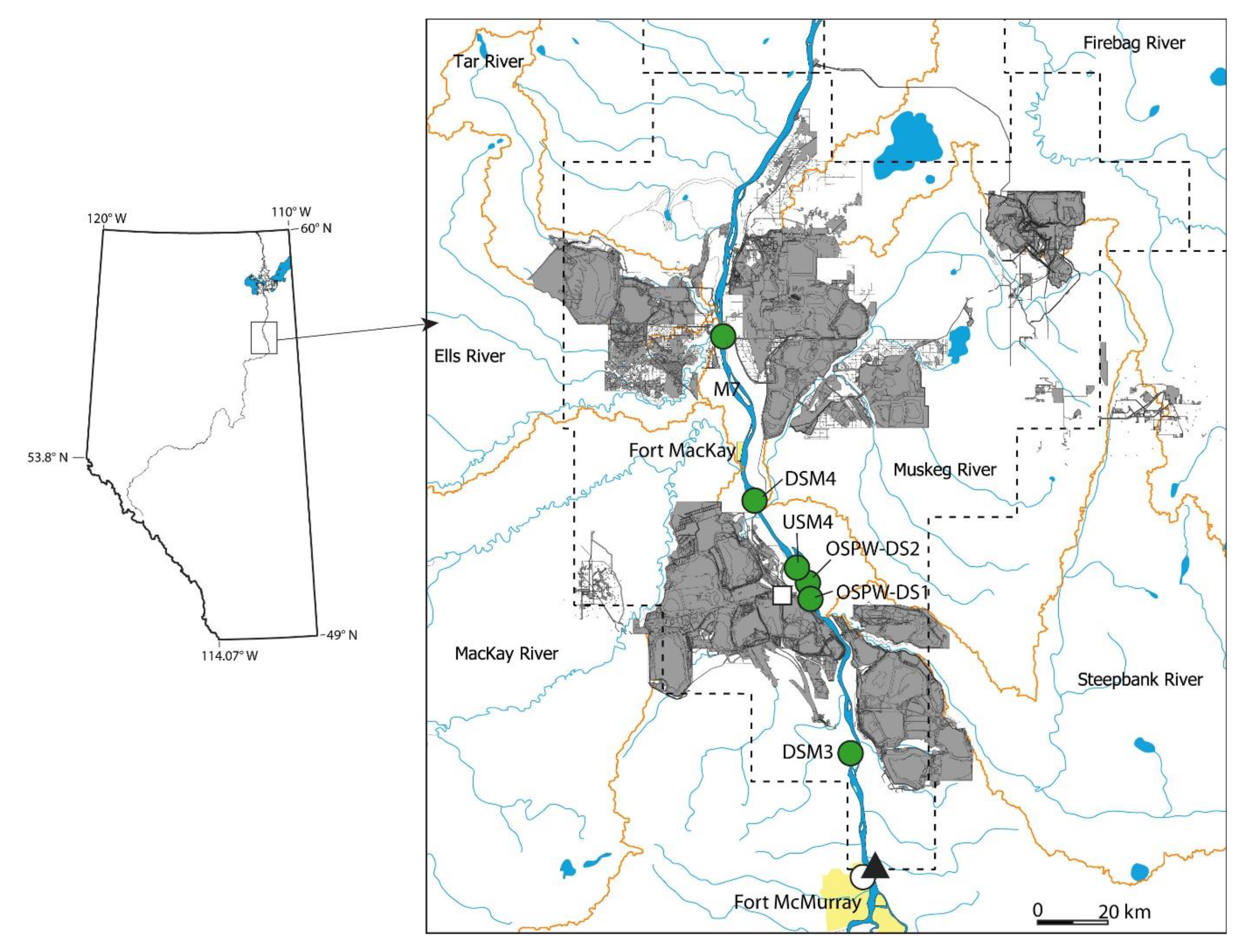
2.1. Fish Collection

White sucker residing in the Athabasca River near oil sands facilities likely over-winter in Lake Athabasca [50], but are resident over the summer. To maximize exposure to local conditions and exposure gradients, white sucker were collected in the Fall of study years at three primary sites. White sucker were collected within the McMurray formation and adjacent to mines (DSM3), and in areas within the McMurray formation and downstream of, and adjacent to, mines (USM4 and DSM4; Figure 1). The DSM3 site is within 20 km of the FMM WWTP outfall. Fish residing at all locations may also be influenced by materials deposited from the atmosphere via the adjacent mining activity. While not initially part of the monitoring studies done as part of the Oil Sands Monitoring program, parallel collections of white sucker were also done during the timespan of this study. These additional collections including an additional year (2014) and additional sites (M7, OSPW DS1, and OSPW DS2). These data were retained for this study and further information is provided below.

The sampling schedule used in this program has been adapted for use in the OSR from the technical guidance for the regulatory Environmental Effects Monitoring (EEM) program (e.g., [51]). Environmental Effects Monitoring programs are based on the periodic collections of fish. In an EEM framework, fish are collected once every 3–4 years during the routine surveillance cycle. We used a modified version of this sampling schedule. In our work, initial collections of fish were done in 2011, 2012, and 2013 to establish existing conditions. The next regularly-scheduled collections were set for 2016 and 2019. Target sample sizes for each site sampled in these years were 20 adult males and 20 adult females. The actual sample sizes for sites, sex, year, and measurement range from 2 to 22 (Supplementary Table S1). Capture success in 2016 was poor, but these data were retained in the current analysis.

Additional fish collections were done in 2014 to support the effect analysis of the Obed Dam breach in the Athabasca drainage (e.g., [52]). The target sample size for these additional collections was 10 fish per site and included additional sampling at a site, M7, farther downstream than the focal sites in this study. While primarily for examining the accumulation of contaminants in the tissues of these fish, measurements of fish health were also done. Although a low sample size, these fish measurements were opportunistically included here. Fish data for other parallel studies were also included here. In 2016, fish were also collected at a site further downstream (M7) in a pilot program to determine the potential benefits of spatially expanding the collections. Additionally, fish were also collected in a second pilot program to document the status of fishes before the potential release of treated oil sands process-affected waters (OSPW DS1, and OSPW DS2; [53]). These additional collections at OSPW DS1 and OSPW DS2 were only done in 2019. While the sample sizes for these additional collections were low, we included these fish by pooling samples into a regional site called “allOSR“. Further steps to account for the potential effect of small sample sizes on this analysis are described in Section 2.3.

Adult female and male white sucker at each of the study locations were collected using boat electrofishing under scientific collection permits issued by Alberta Environment and Parks (11-04841, 12-0467, 13-0445, 14-0456, 16-0811, 19-0420) and following the Canadian Council on Animal Care approved Animal Use protocols (1122, 1315, 1415, 1615 and 1915) issued by the National Water Research Institute Animal Care Committee. Stunned fish were captured using dip nets (approx. 0.5-cm mesh size) and were transported to the portable on-site laboratory for processing. In the mobile laboratory, fork length (FL; ±1 mm), body weight (BW; ±0.1 g), liver weight (LW; ±0.01 g), gonad weight (GW; ±0.01 g), and sex were recorded. Opercula were also removed for aging (±1 y).

2.2. Regression Analyses: Attributing Variance

The focus of this work is on the change in relative GW, LW, and BW in white sucker at individual sites over time in the Athabasca River. We built on previous approaches to examine the gonadosomatic (relative GW), liver-somatic (relative LW), and condition (relative BW) indices in previous fish health studies. The initial approaches were extended to include additional covariates to construct control charts that account for “assignable” and “unassignable” sources of variation [54]. The first analyses of GW, LW, and BW included respective independent variables of BW, carcass weight (CW; BW-GW), and FL only. These initial analyses indicated potentially relevant differences, especially in 2014, and additional structure in residuals (e.g., Figure 2). For example, median summer discharge in 2014 was the lowest among the years in which white sucker were collected (Supplementary Table S2) suggesting this variable may be associated with the health estimates of fish.

To account for the possible influence of environmental covariates, we included temperature, discharge, sewage phosphorus, and precipitation iteratively by examining improved model fits and the magnitude of residual error as additional variables were added. The analysis used median regressions to calculate expected relationships and residual variation for fish collected in all years for a given analysis of sex, site, and measurement. The total sample size for each regression ranged from 59 to 227 (Supplementary Table S1). All quantile regressions were performed using the rq() function in the quantreg package in R [55]. Double bootstrapping was used to estimate the expected ranges of median residuals. All variables were log₁₀ transformed before the analysis.

To account for the potential influence of natural variation on the health of fish, we added surrogates to attribute variability among measurements of the performance of fish populations to their possible sources. First, we added the surrogates of discharge and temperature into the models to account for natural hydrological and climatological effects. The median discharge (D) in the Athabasca River was calculated for 60 days before the collection of individual fish. Water temperature was not available for study locations and the median summer (June, July, and August) air temperature (T) was used as a surrogate. Medians were chosen to control for the influence of outliers. Discharge for the Athabasca River (e.g., DSM3, USM4, DSM4) was obtained from the Fort McMurray gauging station which is upstream of all study locations (Water Survey of Canada Station Number: 07DA001; Figure 1). The data on air temperature was obtained from the Mildred Lake meteorological station (Meteorological Service of Canada Climate ID: 3064528; Figure 1).

Multiple models were initially used to estimate and attribute variation in the indicators of fish health at sites over time. Eight potential model forms were initially developed to describe variation in fish (

Table 1. Forms of original models used to account for the influence of independent variables and environmental covariates of air temperature and discharge on GW, LW, and BW of white sucker; De = Dependent; I = Independent; T = Temperature; D = Discharge; A = Age.

Model Number	Model Form
1	De = I + T + D
2	De = I + T + D + T2 + D2
3	De = I + A + T + D
4	De = I + A + T + D + T2 + D2
5	De = I + A + T + D + D2
6	De = I + T + D + D2
7	De = I + A + D + T + T2
8	De = I + D + T + T2

). Since temperature and discharge are known to affect fish health parameters, these models all included at least T and D. The influence of fish age and squared terms for T and D were also included in some model forms (Table 1). The best model fit was selected using Akaike’s Information Criterion (AIC) and was the basis for conducting subsequent analyses (Supplementary Table S3). Although some differences in AICs were marginal, given the exploratory and retrospective nature of this analysis, we used a strict interpretation of AICs to determine the improvement of models. The T + D models selected for LW and BW of males at DSM4 included age. Of the three male fish captured at this location in 2016, no age was available for one of the fish. Subsequently, for models with environmental covariates, no estimate was made for LW and BW of male fish captured at DSM4 in 2016.

After accounting for T and D, some potentially relevant differences remained in GW, LW, and BW. We performed exploratory analyses to determine the influence of additional factors. First, we augmented the original models fit GW, LW, and BW by site and sex with total phosphorus (P) and squared phosphorus (P²) measured in the final effluent discharged by the FMM WWTP. Phosphorus in final effluent was chosen to capture the potential influence of sewage on fish which has been postulated from recent studies on benthic invertebrates [56]. We represented phosphorus as the mean concentration in the final effluent discharged from the FMM WWTP in the summer (June, July, and August; Supplementary Table S2). A mean was used to define sewage phosphorus because no outliers were present in the dataset available from compliance reporting submitted annually to regulators. Improvement in the model fits by including P and P² were also estimated using AICs. The P and P² coefficients were recorded for those models improved by including these variables.

We further augmented the descriptive models using other available data. The wet and dry deposition has been postulated as a primary effect pathway linking OSIA and the environment [38,57,58]. Furthermore, while the influence of precipitation is correlated with discharge and temperature, these variables are not co-linear (Supplementary Figure S1) suggesting a unique and possible role of local precipitation. After accounting for D, T, and P, we augmented the surviving models with information on precipitation. Mean daily summer (June, July, August) precipitation (Pr) was obtained from the Mildred Lake meteorological station records. Mean precipitation was used because more than 50% of days in June, July, and August of several study years had no precipitation which returned a median of 0. Squared precipitation (Pr²) was also included in the analysis. Improvement in the model fits by additional variables was evaluated using AICs. Coefficients for Pr and Pr² were recorded for those models improved by including these variables. Summer precipitation was chosen to account for annually representative conditions present during the primary growth and tissue maintenance phase of white sucker. Further accounting for remaining variability with more precise or additional descriptors of local influences, including a potential influence of deposition during the winter was not done.

Bootstrapping Procedures: Detecting Potentially Relevant Differences

Residuals were calculated from the best fit models derived through median regressions in each step described above. We compared the occurrence of the observed and expected medians of residuals between a reference period and individual test years. In this analysis, we defined 2011–2013 as the reference period (i.e., expected)) and the test (i.e., observed) years were 2014, 2016, and 2019.

The expected range of residuals for each test year was calculated from the residuals observed during the reference period using a double bootstrapping procedure. Double bootstrapping is typically used to correct coverage errors of confidence intervals which can occur with single bootstraps [59,60]. The double bootstrap was used to calculate the central 95% confidence intervals (CIs) of medians and their 95% CIs for the within-site analyses. These intervals provide an estimate of where residuals will occur if the sources of variation described in the error term of the model were stable between reference (2011–2013) and test (2014–2019) periods while also accounting for sample size differences for each test analysis.

The specific procedure as implemented here is described in detail elsewhere [61], but briefly, the number of resamples (m) was set to the sample size of the sex, site, measurement, and test year being considered. During the first bootstrap, X* was generated by drawing m samples with replacement from the empirical distribution X. In these analyses, the empirical distribution was set to the sex, site, and measurement from 2011 to 2013. A second bootstrap was performed by again drawing m samples with replacement from X* to generate X**. The number of first-level bootstraps (B) was set to 4999 and the number of second-level bootstraps (C) was set to 999.

Double bootstrapping yields 95%CI of 95%CI and is presented here using two statistical descriptors. The narrowest estimates are the 2.5 and 97.5 percentiles (referred to here as percentiles proper). The wider estimates for each percentile proper are the corrected percentiles and represent the outer boundaries of the 95%CI of the 95%CI. Double bootstrapping was not used for the observed medians to increase the sensitivity of the analyses. We estimated the observed distributions of median residuals for each sex, site, year, and measurement combination using a single bootstrap where B was set to 99,999. These were done for both reference and test years.

Calculating 95%CIs for medians using bootstrapping can perform poorly [62]. For m between 3 and 14, a normal distribution was fit to the residuals. For m greater than 14, a Gaussian Kernel smoother was used to estimate the 95%CIs of medians. The estimated bandwidth of the Kernel was calculated using the dpik() function in the KernSmooth package [63] in R. Fourteen was used as a threshold to reduce the probability of duplicating bootstrap datasets using our choice of B and C and the failure of dpik() to estimate bandwidth for smaller sample sizes. Custom scripts were written in R for single and double bootstrapping. These scripts are provided in the Supplementary Materials.

2.3. Data Interpretation

Among the analyses here, the low sample sizes in some years, especially among males, affect the certainty of the results and the conclusions. However, to extract useful information from these data, several steps were taken to account for the low sample sizes of fish captured during the test period. First, sites with fewer than 3 fish were included in the regression modeling but were not included in the analyses to detect change. To account for the information contained in these fish and sites where sample sizes were less than 3, a regionally pooled site, including fish captured throughout the OSR reach (DSM3 to M7) was created for analyses here. This regional site is called “allOSR”.

The rule-set for ascribing the potential occurrence of a large difference was also modified to account for the small sample sizes. We used the occurrence of the observed test medians outside the 2.5 or 97.5 percentile proper from the expected ranges of the median residual to detect potentially relevant differences used in earlier work [61]. In contrast to the earlier approaches [61], we did not use the variability of the observed medians to ascribe relevance. Our approach here inflates the false positive rate but is suitable for our purposes of identifying potentially relevant differences, to identify patterns supporting the postulated linkages between local stressors and the health of fish in the Athabasca River, and for informing the methods for both the study design and the analysis of future monitoring data. Another component was also used in our interpretation of data. Following techniques of regression diagnostics, we also qualitatively inspected the plots of the annual median residuals for evidence of hidden or undescribed structure, such as monotonic trends over time.

3. Results

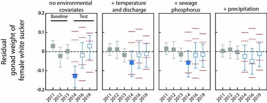
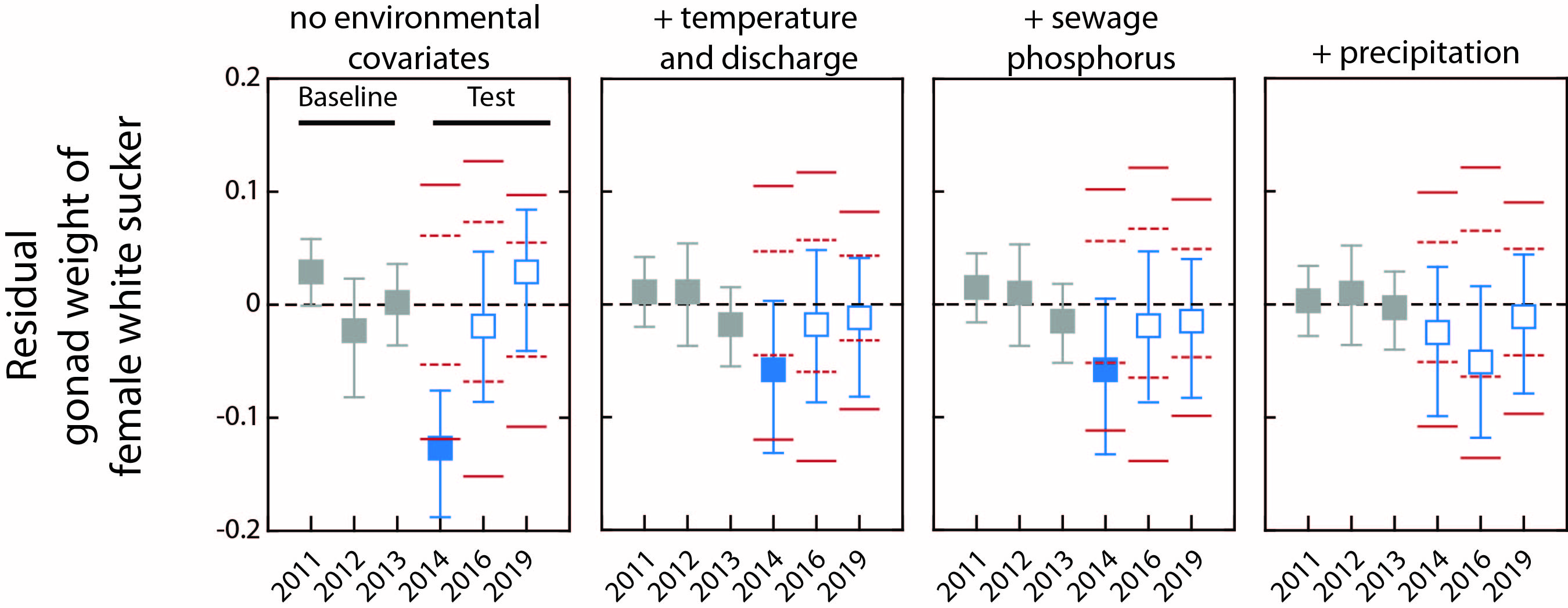
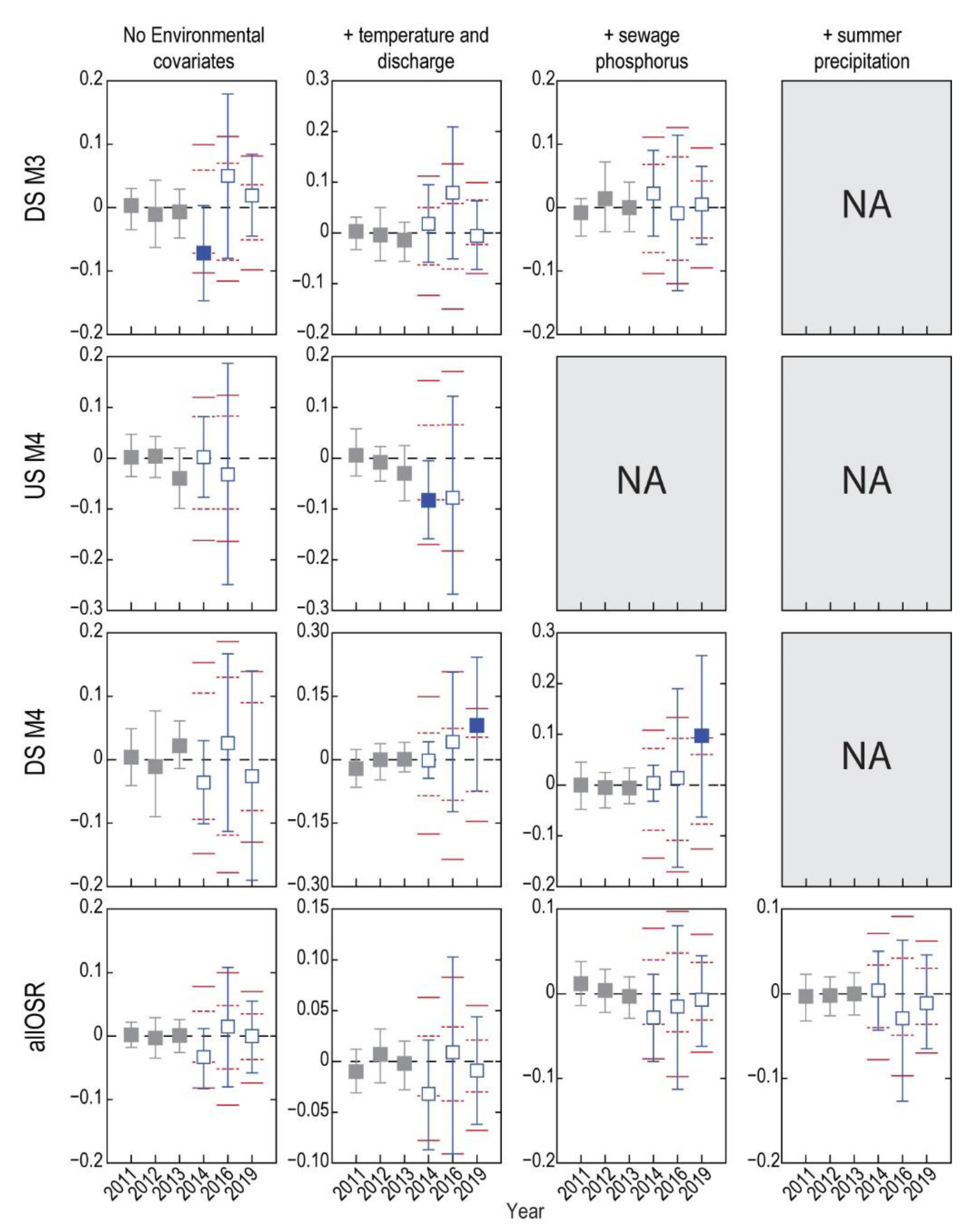
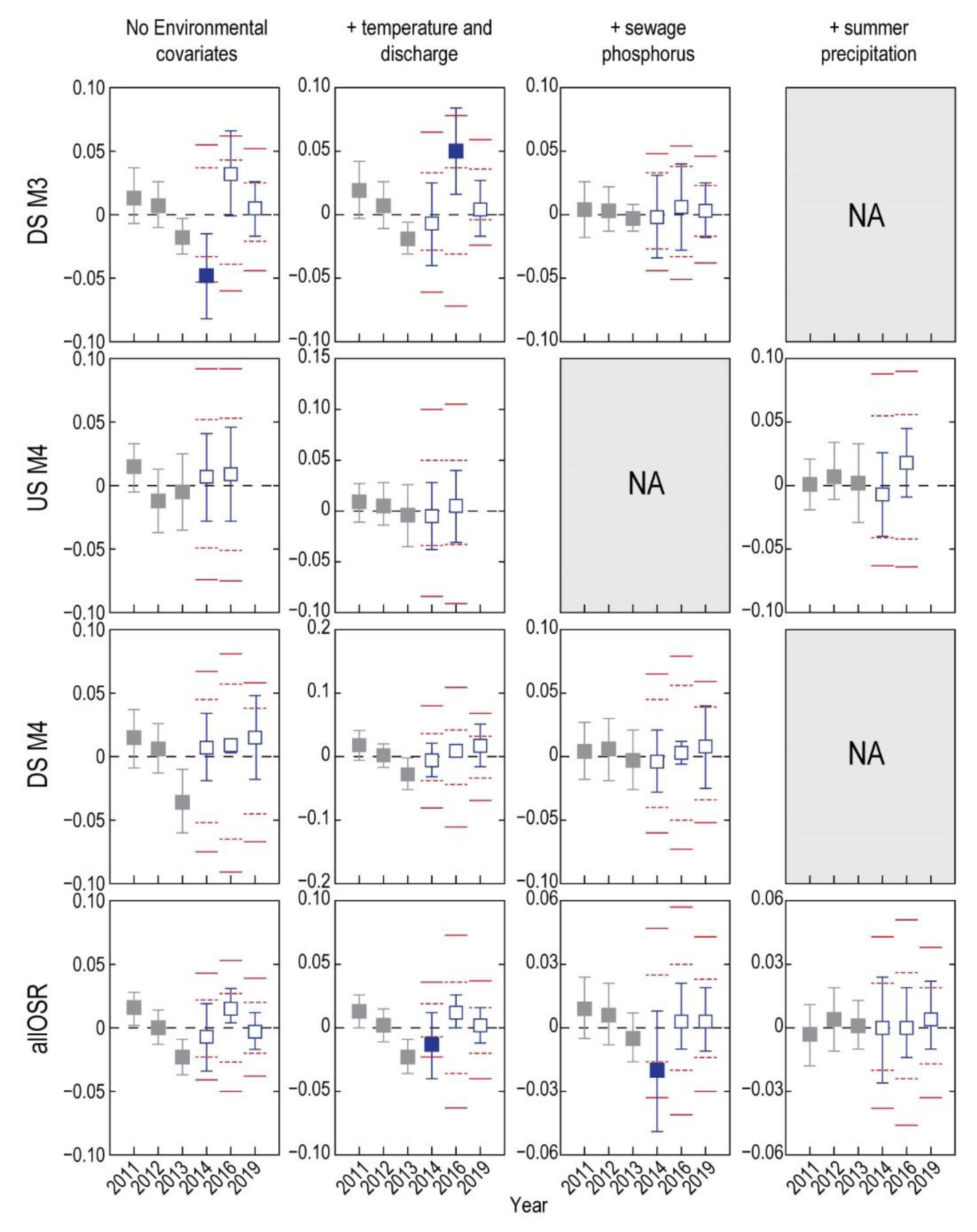
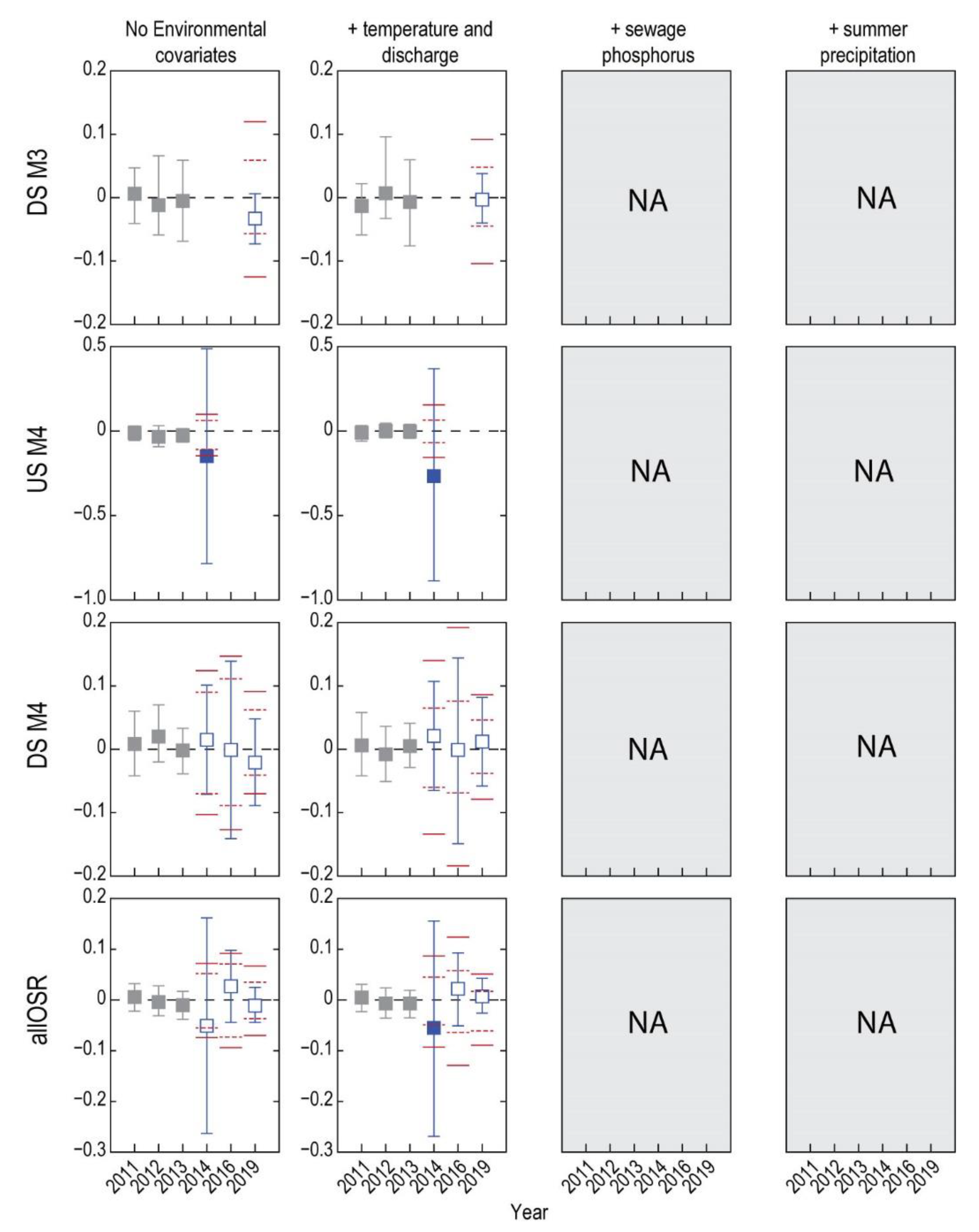
3.1. Analysis of Fish without Environmental Covariates

We first examined the potential occurrence of relevant differences in analyses done without environmental covariates (Figure 2, Figure 3, Figure 4, Figure 5, Figure 6 and Figure 7). In these analyses, several potentially relevant differences were found, including relative GW (Figure 2), LW (Figure 3, and BW (Figure 4) in females captured at DSM3 in 2014. Observed median GW was also lower than expected at the allOSR site in 2014 (Figure 2). While statistically uncertain, potentially large differences were also observed in GW of males at USM4 (Figure 5), LW of males from the allOSR location in 2019 (Figure 6), and in BW of males at USM4 and allOSR in 2014 (Figure 7). Patterns indicating additional structure, such as the progressive increase in the residual error of GW of females from 2014 to 2019 at DSM3, was also apparent in these data (Figure 2).

3.2. Do Discharge and Temperature Account for Changes in Fish?

After accounting for the potential influence of D and T, the potentially relevant differences in fish changed compared to the results of models that did not include any environmental covariates (Figure 2, Figure 3, Figure 4, Figure 5, Figure 6 and Figure 7). When D and T were included in these models, the potentially relevant differences in GW, LW, and BW of females captured at DSM3 in 2014 disappeared (Figure 2, Figure 3 and Figure 4). A potential difference in LW in males from the regional allOSR site in 2019 also disappeared after including T and D (Figure 6). In contrast, potentially relevant differences in GW of females captured at allOSR in 2014 persisted after including T and D (Figure 2). Potentially relevant differences also persisted in males after accounting for T and D. These differences in males all occurred in 2014 and included GW and BW at USM4 and BW at the allOSR location (Figure 5 and Figure 7).

While potentially relevant differences disappeared and others persisted, new differences also appeared after including T and D in the descriptive models. These new and potentially relevant differences were observed in BW of females captured at DSM3 in 2016 (Figure 4), LW in females captured at USM4 in 2014 and at DSM4 in 2019 (Figure 3), BW of regional (allOSR) females in 2014 (Figure 4), and GW of males from the regional allOSR location in 2014 (Figure 4). Additional patterns in residuals over time, such as the gradual increase in residual LW in females captured at DSM4 over time (Figure 3) and annual variability of median residuals of GW of females at DSM3 (Figure 2) suggested other structural variables may be influencing these data.

3.3. Does Including Sewage Phosphorus Improve the Descriptive Models?

We next examined the potential effect of sewage phosphorus on fish captured in the Athabasca River. Of the 24 initial T + D models, fourteen were not improved by including P or P + P² (

Table 2. AICs for original models (See Supplementary Table S1) supplemented with temperature (T), discharge (D), sewage phosphorus (P), and precipitation (Pr) on residual dependent variables (DV) of gonad weight (GW), liver weight (LW), and body weight (BW) by sex, site, and year; AICs in bold indicate the improvement of the T + D model per column variable; best fit models for all evaluated coefficients shown as underlined AICs; coefficients for improved models using P and Pr also shown.

Sex	Site	DV	AICs					Coefficients
			T + D	+P	+P + P2	+Pr	+Pr + Pr2	P	P2	Pr	Pr2
F	DSM3	GW	−124.65	−126.62	−130.41	−133.04	−131.34	2.26	1.89	−2.42
		LW	−179.87	−177.9	−180.35	−179.21	−177.49	1.83	1.62
		BW	−306.63	−306.1	−329.13	−327.66	−326	1.13	0.98
	USM4	GW	−71.92	−71.18	−74.18	−73.92	−71.93	−2.11	−1.78
		LW	−124.14	−123.95	−122.03	−123.77	−122.03
		BW	−208.99	−207.68	−205.78	−209.64	−207.77			−0.05
	DSM4	GW	−115.53	−114.77	−112.8	−114.82	−112.85
		LW	−124.69	−127.85	−126.84	−127.61	−125.62	−0.09
		BW	−236.00	−236.95	−244.1	−249.06	−247.09	0.59	0.47	−0.64
	allOSR	GW	−302.88	−301.64	−301.47	−302.22	−305.71			0.71	−1.94
		LW	−447.3	−448.59	−446.61	−447.88	−458.94	−0.07		2.62	−5.86
		BW	−776.94	−776.9	−787.08	−802.03	−804.64	0.55	0.45	0.07	−0.64
M	DSM3	GW	−132.67	−131.59	−129.67	−131.6	−130.94
		LW	−104.96	−110.22	−112.28	−110.69	−110.49	−9.99	−9.07
		BW	−258.31	−256.9	−254.93	−256.9	−254.99
	USM4	GW	−101.75	−99.93	−98.04	−99.97	−98.02
		LW	−120.5	−119.41	−117.56	−119.51	−120.36
		BW	−204.03	−204.42	−204.02	−202.63	−204.73	−0.04		0.56	−1.42
	DSM4	GW	−184	−182.24	−180.25	−182.26	−180.61
		LW	−149.44	−147.5	−146.36	−147.47	−145.61
		BW	−303.15	−302.18	−301.17	−302.42	−301.77
	allOSR	GW	−436.02	−434.08	−433.31	−434.38	−432.42
		LW	−390.82	−389	−387.42	−388.84	−387.02
		BW	−795.28	−793.58	−792.18	−793.41	−796.82			−0.19	−0.51

). However, including P or P + P² improved ten (Table 2). Among these ten, eight of the improved models occurred in female fish suggesting a larger influence of sewage P on females compared to males; however, this result should be viewed cautiously given the small sample sizes of male fish after 2013 available for analysis in this study. Among the improved models, three improved by including only P. These three improved models were BW of male fish from USM4 and LW in females from DSM4 and regionally using the allOSR site. Among these three models, the P coefficients all indicated a negative effect on indicators of fish health (Table 2).

The potential influence of P + P² were also observed in white sucker captured in the Athabasca River. Among the seven models improved by including P and P², both positive (e.g., GW of DSM3 females) and negative coefficients of P² (e.g., GW of USM4 females) relationships were identified (Table 2). Among females captured at DSM3, all three variables examined here, GW, LW, and BW were potentially affected by P². These P² coefficients were all positive suggesting initial declines in fish parameters followed by eventual increases in concentration of P in final effluent discharged from the FMM WWTP. Potnetial effects of P+P² on BW were observed at three spatial locations (Table 2). At these three sites, positive coefficients of P² were observed suggesting a common mechanism (Table 2). In contrast, the effect of P² on LW at DSM3 showed opposite patterns of influence by sex. While a positive P² coefficient was found at DSM3 in LW of females, a negative coefficient was found in LW of males captured at the same site. These and other results suggest a potentially different mechanism of sewage effects by sex, but also spatially heterogeneous responses. However, these results may also be affected by low sample sizes of male fish and should be considered hypothetical without further dedicated studies.

3.4. What Is the Status of Fish Health after Accounting for Sewage Phosphorus?

Among the ten models improved by the inclusion of sewage P (Table 2), no new differences appeared, but one disappeared and three persisted (Figure 2, Figure 3, Figure 4, Figure 5, Figure 6 and Figure 7). A potential differences BW of females captured at DSM3 in 2016 which were apparent after accounting for T and D disappeared when sewage P was added to the models (Figure 4). However, potentially relevant differences in LW of females captured at DSM4 in 2019 (Figure 3), BW of females from the allOSR site in 2014 (Figure 4), and BW of males captured at USM4 in 2014 persisted (Figure 7). The occurrence of these differences is likely affected by uncertainty but suggest a potential role of additional stressors in the Athabasca River.

While potentially relevant differences were observed in white sucker after accounting for sewage P, the patterns in residuals also suggested further structural variables may be affecting white sucker residing in the Athabasca River. The most notable example was observed at the regional allOSR location in BW of females (Figure 4).

3.5. Does Summer Precipitation Influence the Health of Fish?

Based on the occurrence of differences and potential patterns in residuals, we performed further analyses using local summer precipitation. In these analyses, we found evidence suggesting a role of precipitation or an associated variable in explaining variation in white sucker captured in the Athabasca River between 2011 and 2019 (Table 2). Although some were cases marginal, such as BW of males captured at USM4, eight models were improved by Pr or Pr². Among these eight, five were improved after including P and the remainder, such as female BW at USM4 (Figure 4) did not include P. Among all models improved by including Pr, females examined regionally (i.e., allOSR) showed negative Pr² coefficients suggesting initial increases in residual GW, LW, and BW followed by eventual decreases as precipitation increases (Table 2). These relationships were repeated in BW of males captured at USM4 and regionally (allOSR; Table 2). Where only Pr improved the models, negative coefficients suggest lower GW of females captured at DSM3 and BW of females captured at USM4 and DSM4 with increases in precipitation. While mostly subtle indications of influence were found when Pr and Pr + Pr² improved model fits, sixteen models were not improved by including Pr or Pr + Pr².

3.6. What Is the Status of Fish Health after Accounting for Summer Precipitation?

Including Pr or Pr + Pr² improved model fits in white sucker captured in the Athabasca River. After accounting for the influence of Pr, two differences in females disappeared (Figure 3 and Figure 4). A potentially relevant difference in females present after accounting for T and D and where P improved the model fit, BW in at allOSR in 2014, disappeared after including Pr (Figure 4). Where P did not improve the model fit, GW in females captured at allOSR in 2014, including Pr also eliminated this potentially relevant difference (Figure 2). In contrast to females where differences were eliminated by including Pr, two potentially relevant differences remained in males (Figure 7). Both were observed in BW of male fish captured in 2014 and were observed at USM4 and the regional allOSR location (Figure 7). Importantly, the improved fit by including Pr occurred with the T + D + P model for USM4 (Figure 7) and the T + D model for the allOSR fish (Figure 7).

4. Discussion

Identifying change and attributing cause are two goals of environmental monitoring programs [64]. Annual variation in estimates of population performance of white sucker captured in the Athabasca River near oil sands developments was apparent in previous work, suggesting the potential influence of structural variables not included in the initial analyses. The initial analyses of T and D done here also suggested additional structure remained in the data. Two of these potential additional sources are domestic sewage and atmospheric deposition. We used data from the FMM WWTP (P) and precipitation (Pr) to approximate the influences of these sources. After accounting for T, D, and P, few potentially relevant differences were observed, but some remained, such as the LW of females in 2019 captured at DSM4. Further analyses using models improved by precipitation removed two potentially relevant differences in females, but two differences in BW of males captured in 2014 at the USM4 and the regional allOSR locations remained. Additionally, 3 potentially relevant differences in BW of males were also observed in 2014, GW of males from the allOSR location and USM4 in 2014, and LW of females from both DSM4 in 2019 and USM4 in 2016 remained and were not attributable to P or Pr. The remaining differences in 2014 may be attributable to the Obed Mine dam breach [52] or, more likely, to the low statistical power attributed to the small sample size in males captured in that year. Where present, the small sample sizes have under-powered the analyses here suggesting important effects have been missed. However, the results here are also consistent with the expected natural and human influences on fish residing in the Athabasca River.

Among the analyses to detect anthropogenic influence performed here, model improvements (while in some cases marginal) suggest the potential influence of sewage P in the Athabasca River captured at some locations. This influence is especially apparent in the improved model fits in female GW, LW, and BW collected at DSM3. This site is downstream of the FMM WWTP outfall and where we would expect sewage influences to be most apparent. Other researchers have also suggested changes in both the benthic invertebrate communities and fish populations in the Athabasca River may be associated with sewage inputs, including the discharge of nutrients [33,40,45,46,56]. While both the concentration of P and ammonia in the final effluent from the FMM WWTP has been declining over time (Supplementary Figure S2) enrichment may be affecting fish in the Athabasca River. Enrichment effects of sewage are common in Canadian waters [65], but groundwater and atmospheric emissions are also potential sources of nutrients in the OSR [66,67].

Among the observed model improvements (while some are marginal) the potential relationships with sewage P were not homogenous throughout the study region. Spatially heterogenous effects in females related to P throughout the study area suggest hypothetical but changing importance of multiple components in the sewage mixture. Assuming the observed patterns are not affected by sample size, another observation challenging a simple mechanism of sewage effects is the contrasting direction of P² in residual LW in males and females captured at DSM3. Sewage effluents are complex mixtures and our data also indicate multiple mechanisms may be operating simultaneously at single locations. For example, Pr influence at DSM3 suggests an additional role of sewage via overflows of treatment systems during high precipitation events. Responses in fish exposed to sewage [68] or potent components of sewage [69] can be complex but commonly includes endocrine disruption. However, some bituminous compounds are also endocrine disruptors [70]. Further analyses of the potential endocrine effects in the lower Athabasca River may be warranted. The incremental addition of domestic sewage from industrial facilities, including mines and potentially workcamps, and Fort MacKay as the Athabasca flows through the study area may also influence these results. While sources and mechanisms may currently be obscure, our analyses suggest accounting for the presence of sewage improves the ability to detect the influence of OSIA.

While other potential sources of variation near oil sands facilities are also possible, such as minor delivery of CoCs via seepage of water from tailings ponds or the substantive influence groundwaters naturally in contact with bitumen [21,34,71,72], within the oil sands region, atmospheric deposition is considered a primary exposure pathway linking industrial development and the ambient environment [58]. For example, work in the OSR also suggests rain is an efficient scavenger of some contaminants, such as Hg [57] and polyaromatic compounds [73]. Other research in the OSR also suggests the potential accumulation of CoCs originating from OSIA in ombrotrophic bogs and other landforms or receptors [31,74] via wet and dry deposition [75,76]. Our data augments this earlier work and suggests a role of wet and dry deposition in the health of fish residing in the Athabasca River. This contention is supported by additional data from the OSR. Studies have found the highest levels of atmospheric deposition in the Athabasca River Valley ([67]; Supplementary Figures S3 and S4). This low-relief area may accumulate high concentrations of CoCs which may be eventually delivered to the Athabasca River following or during protracted or intense rain events. While our analyses focused on the influence of summer precipitation, researchers have also identified pulses of CoCs and episodic acidity during high flow events associated with snowmelt in tributaries [35,77] and with particular phases of industrial activity, including construction [26]. We estimated the potential influence of atmospheric deposition on fish using summer precipitation and found a possible association in fish captured at some locations. The plausible influence of wet and dry deposition on fish is suggested, weakly in some cases, by our analyses here, but the ability to rigorously evaluate these hypotheses with existing data is limited. For example, estimates of precipitation would not account for direct dry deposition to waterbodies. Regardless of these challenges, our work strongly supports the pursuit of dedicated data collections to examine the potential influence of wet and dry deposition on aquatic organisms.

Atmospheric emissions from OSIA near our study locations are common and persistent, but our analyses did not attempt to separate the wet or dry deposition or its particular sources. In the OSR, the largest contributors to wet and dry deposition are industrial development, urban activity, and forest fires [38]. Urban signals are clear in some analyses [38], but they have not been a major focus of study in the region. In contrast, wildfires are common in the Boreal Forest [78] and two large spring fires occurred during our study period: 2011 and 2016 [79,80]. Recent work in the OSR following the 2016 Horse River fire suggests relationships between precipitation events and water chemistry in burned watersheds [36]. Furthermore, data on the concentrations of biotransformation products of PACs in the bile of northern pike (Esox lucius) collected in the summer of 2011 were also elevated following the Richardson Fire [37]. While similar spatial and temporal patterns are somewhat supported by PAHs measured in the muscle of these same fish [81], no patterns were apparent in concentrations of metals [82]. These data support the potential role of forest fires in the associations between the performance of fish health and precipitation. Further considering the effects of forest fires in analyses of regional impacts of OSIA may be necessary.

Sample sizes are limited in some years, especially in males, but other challenges also require additional consideration in evaluating a potential relationship between precipitation and the health of fish. Given the challenges of including environmental covariates in a retrospective analysis where no new data can be collected [61], some of the variations we observed in fish could be misattributed to precipitation or are properly attributed to precipitation, but through a mechanism not yet discussed. For example, a weak but non-zero relationship between precipitation and discharge (Supplementary Figure S1) suggests a small effect of discharge downstream of the Fort McMurray gauge is embedded in Pr. This contention is supported by additional research [35,83] and by additional data available for the region. On average, 90% of flow present in the Athabasca River at the Embarras Airport gauging station (DD001) which is downstream of all development [84] is already present in the channel when river water reaches the gauging station at Fort McMurray (Supplementary Figure S5). However, this value ranges from 33 to 129% (Supplementary Figure S5). Mines withdraw water and alter the hydrology of watersheds before, during, and after operation [26,30,34,35] which may affect the natural occurrence of CoCs [39,85] or alter the delivery of any industrially-derived substances to tributaries [11,35], but these activities occur downstream of the Fort McMurray gauging station. This information suggests potential influences of local development on local discharge (but not contributing to our estimate of D) may be occurring [26]. Consequently, any influence of this difference between local flow at study locations and D may be encapsulated in Pr. These influences may, therefore, manifest as linkages between fish health and Pr.

The estimate of discharge, D, may, however, contain some information on CoCs. The water already flowing in the Athabasca River channel at Fort McMurray delivers an estimated CoC load that is 11–30 times higher than the estimated total loading from the Steepbank, Muskeg, MacKay, Ells, and Firebag Rivers [47]. While a detailed source attribution study of CoCs has not been done for waters collected in the Athabasca River upstream of Fort McMurray, the majority of these contaminants do not likely originate from OSIA. However, some CoCs may be transported via the atmosphere to areas of the basin upstream of the gauge. There may also be influences originating from operations south for Fort MacMurray (and the Fort McMurray gauging station) in the Horse, Hangingstone, and Christina watersheds.

Similar to discharge, the temperature was used here as a natural stressor that can affect the performance of fish populations [43,86,87]. Characterizing the precise nature of the relationships between wild fish and variables, such as discharge and temperature in a retrospective analysis is, however, often challenging [61]. Similar to Pr and D, T is likely a complex descriptor of variation and may be influenced by industrial practices. Here we used air temperature, and while not dictated by OSIA, there may be some local and transient influence, including effects of heat sinks and the direct and indirect carbon emissions from oil sands developments [88]. However, fish in the study area may be exposed to treated domestic waters released into the Athabasca River from industrial and municipal facilities [32]. The influence of these warm effluents, if present, is likely greater than any direct effect of industry on air temperature and is likely absent from our estimate of T. Instead, an effect of these effluents, through potentially minor, may be misattributed to sewage P or Pr or may contribute to the remaining residual variation, such as LW of females captured at DSM4 in 2019.

Our analyses and additional literature support the role of anthropogenic activity on the health of fish, but the physiological mechanisms were not indicated through our work. For example, water sampled from rivers during these pulses, although they can elevate risks in sensitive life stages of fish [75], did not elicit mortality in lab studies using field-collected waters [27]. However, sub-lethal effects may be possible. Our data support the occurrence of sublethal effects in white sucker and precipitation. Physiologically, the coefficients of Pr and Pr + Pr² suggest a potential decline in health parameters with the highest precipitation which may be associated with the delivery of contaminants. This is supported by the induction of liver detoxification enzymes, but the role of precipitation in those data is uncertain [33]. However, lower precipitation also suggests declines in health parameters when P² was deemed relevant by AIC. While the role of lower concentrations of CoCs or changes in constituents in this pattern is not clear, less precipitation may be associated with less favorable conditions, including fewer interactions with the landscape. Nutrients deposited to the landscape from the atmosphere [67] and the productivity of fish may also be linked. Better designing studies to document the linkages between fish health and wet and dry deposition may be beneficial for regional monitoring.

Our analyses here suggest various roles of human activity and natural stressors on the health of fish, but additional caveats are required. For example, the criteria we used to identify changes are not definitive and any remaining “potentially relevant differences” are also potentially false positives. There are challenges with how far these results can be extrapolated, but this work also provides tools and direction for future monitoring of white sucker in the mainstem Athabasca and partition variance into assignable and unassignable sources [54]. Our work especially suggests the importance of including environmental covariates into surveillance monitoring in areas like the OSR where most influences are diffuse. If novel sources of variability emerge, or the existing relationships described with the covariates we have used changes, the observed variability may begin to drift out of the expected range or show other improbable patterns [82]. However, additional work to better test our hypotheses may also be used. These include dedicated studies in tributaries, collecting more precise information on environmental covariates, expanding the covariate list, or potentially by adopting non-lethal sampling to increase the frequency of sampling [89] and boosting the sensitivity of the analyses. However, the current approach could also be made more sensitive by using alternative selection rules to detect differences or through the potential estimation of any influence of spring melt. The approach used here may also be useful for additional monitoring of fish done in the OSR tributaries.

5. Conclusions

Determining the influence of OSIA on aquatic biota is a goal of regional monitoring in northeastern Alberta. In this analysis, we attempted to account for extraneous sources of variation, initially including D and T. While sample sizes are small between 2014 and 2019, including D and T improved the descriptive models used to evaluate the potential occurrence of additional sources of variation. Improvements in models by including sewage P and Pr, although in some cases marginal, suggested the potential influence of these factors on fish residing at some sites in the Athabasca River downstream of Fort McMurray. Although important effects were likely missed and others identified here are uncertain, hypothetical effects remain which will be important for future collections and analyses during surveillance monitoring. For example, sewage may be affecting fish in the Athabasca River through nutrient enrichment and endocrine disruption. Precipitation may also be affecting fish through the delivery of contaminants originating from multiple sources, including anthropogenic activity. While previously postulated, the analyses presented here support the plausible linkage between health estimates of wild fish and wet and dry deposition in the OSR, irrespective of source. However, these influences did not appear uniform across sex or sites. While extrapolating our results requires caution, further analyses to focus, improve, and verify the occurrence, extent, and magnitude of these hypothesized relationships is warranted.

References

1. Percy, K.E. Geoscience of Climate and Energy 11. Ambient Air Quality and Linkage to Ecosystems in the Athabasca Oil Sands, Alberta. Geosci. Can. 2013, 40, 182–201. [Google Scholar] [CrossRef] [Green Version]
2. Schindler, D. Tar sands need solid science. Nat. Cell Biol. 2010, 468, 499–501. [Google Scholar] [CrossRef] [PubMed]
3. Cho, S.; Sharma, K.; Brassard, B.W.; Hazewinkel, R. Polycyclic Aromatic Hydrocarbon Deposition in the Snowpack of the Athabasca Oil Sands Region of Alberta, Canada. Water Air Soil Pollut. 2014, 225, 1–16. [Google Scholar] [CrossRef]
4. Edgerton, E.S.; Hsu, Y.-M.; White, E.M.; Fenn, M.E.; Landis, M.S. Ambient concentrations and total deposition of inorganic sulfur, inorganic nitrogen and base cations in the Athabasca Oil Sands Region. Sci. Total Environ. 2020, 706, 134864. [Google Scholar] [CrossRef] [PubMed]
5. Gopalapillai, Y.; Kirk, J.L.; Landis, M.S.; Muir, D.C.G.; Cooke, C.A.; Gleason, A.; Ho, A.; Kelly, E.N.; Schindler, D.W.; Wang, X.; et al. Source analysis of pollutant elements in winter air deposition in the Athabasca Oil Sands Region: A temporal and spatial study. ACS Earth Space Chem. 2019, 3, 1656–1668. [Google Scholar] [CrossRef]
6. Landis, M.S.; Pancras, J.P.; Graney, J.; Stevens, R.K.; Percy, K.; Krupa, S.V. Receptor modeling of epiphytic lichens to elucidate the sources and spatial distribution of inorganic air pollution in the Athabasca Oil Sands Region. In Alberta Oil Sands, 1st ed.; Percy, K.E., Ed.; Elsevier Ltd.: Oxford, UK, 2012; Volume 11, pp. 427–467. [Google Scholar]
7. Shotyk, W.; Belland, R.; Duke, J.; Kempter, H.; Krachler, M.; Noernberg, T.; Pelletier, R.; Vile, M.A.; Wieder, K.; Zaccone, C.; et al. Sphagnum mosses from 21 ombrotrophic bogs in the Athabasca Bituminous Sands Region show no significant atmospheric contamination of “Heavy Metals”. Environ. Sci. Technol. 2014, 48, 12603–12611. [Google Scholar] [CrossRef]
8. Korosi, J.; Irvine, G.; Skierszkan, E.; Doyle, J.; Kimpe, L.; Janvier, J.; Blais, J. Localized enrichment of polycyclic aromatic hydrocarbons in soil, spruce needles, and lake sediments linked to in-situ bitumen extraction near Cold Lake, Alberta. Environ. Pollut. 2013, 182, 307–315. [Google Scholar] [CrossRef]
9. Munkittrick, K.R.; Arciszewski, T.J. Using normal ranges for interpreting results of monitoring and tiering to guide future work: A case study of increasing polycyclic aromatic compounds in lake sediments from the Cold Lake oil sands (Alberta, Canada) described in Korosi et al. (2016). Environ. Pollut. 2017, 231, 1215–1222. [Google Scholar] [CrossRef]
10. Schindler, D.W. Geoscience of climate and energy 12. Water quality issues in the Oil Sands Region of the Lower Athabasca River, Alberta. Geosci. Can. 2013, 40, 202–214. [Google Scholar] [CrossRef]
11. Birks, S.; Cho, S.; Taylor, E.; Yi, Y.; Gibson, J. Characterizing the PAHs in surface waters and snow in the Athabasca region: Implications for identifying hydrological pathways of atmospheric deposition. Sci. Total Environ. 2017, 603, 570–583. [Google Scholar] [CrossRef]
12. Conly, F.M.; Crosley, R.W.; Headley, J.V.; Quagraine, E.K. Assessment of metals in bed and suspended sediments in tributaries of the Lower Athabasca River. J. Environ. Sci. Health Part A 2007, 42, 1021–1028. [Google Scholar] [CrossRef]
13. Dolgova, S.; Popp, B.N.; Courtoreille, K.; Espie, R.H.; MacLean, B.; McMaster, M.; Straka, J.R.; Tetreault, G.R.; Wilkie, S.; Hebert, C.E.; et al. Spatial trends in a biomagnifying contaminant: Application of amino acid compound-specific stable nitrogen isotope analysis to the interpretation of bird mercury levels. Environ. Toxicol. Chem. 2018, 37, 1466–1475. [Google Scholar] [CrossRef] [PubMed]
14. Evans, M.; McMaster, M.; Muir, D.; Parrott, J.; Tetreault, G.; Keating, J. Forage fish and polycyclic aromatic compounds in the Fort McMurray oil sands area: Body burden comparisons with environmental distributions and consumption guidelines. Environ. Pollut. 2019, 255, 113135. [Google Scholar] [CrossRef]
15. Evans, M.S.; Talbot, A. Investigations of mercury concentrations in walleye and other fish in the Athabasca River ecosystem with increasing oil sands developments. J. Environ. Monit. 2012, 14, 1989–2003. [Google Scholar] [CrossRef] [PubMed]
16. Glozier, N.E.; Pippy, K.; Levesque, L.; Ritcey, A.; Armstrong, B.; Tobin, O.; Cooke, C.A.; Conly, M.; Dirk, L.; Epp, C.; et al. Surface Water Quality of the Athabasca, Peace and Slave Rivers and Riverine Waterbodies within the Peace-Athabasca Delta; Oil Sands Monitoring Program Technical Report Series No. 1.4; Government of Alberta: Edmonton, AB, Canada, 2018; ISBN 9781460140284. [Google Scholar]
17. Jautzy, J.J.; Ahad, J.M.E.; Hall, R.I.; Wiklund, J.A.; Wolfe, B.B.; Gobeil, C.; Savard, M.M. Source apportionment of background PAHs in the Peace-Athabasca Delta (Alberta, Canada) using molecular level radiocarbon analysis. Environ. Sci. Technol. 2015, 49, 9056–9063. [Google Scholar] [CrossRef] [PubMed]
18. Klemt, W.H.; Kay, M.L.; Wiklund, J.A.; Wolfe, B.B.; Hall, R.I. Assessment of vanadium and nickel enrichment in Lower Athabasca River floodplain lake sediment within the Athabasca Oil Sands Region (Canada). Environ. Pollut. 2020, 265, 114920. [Google Scholar] [CrossRef]
19. Libera, N.; Summers, J.C.; Rühland, K.M.; Kurek, J.; Smol, J.P. Diatom assemblage changes in shallow lakes of the Athabasca Oil Sands Region are not tracking aerially deposited contaminants. J. Paleolimnol. 2020, 64, 257–272. [Google Scholar] [CrossRef]
20. Pilote, M.; André, C.; Turcotte, P.; Gagné, F.; Gagnon, C. Metal bioaccumulation and biomarkers of effects in caged mussels exposed in the Athabasca oil sands area. Sci. Total Environ. 2018, 610–611, 377–390. [Google Scholar] [CrossRef]
21. Roy, J.; Bickerton, G.; Frank, R.; Grapentine, L.; Hewitt, L. Assessing risks of shallow riparian groundwater quality near an oil sands tailings pond. Ground Water 2016, 54, 545–558. [Google Scholar] [CrossRef]
22. Shotyk, W.; Appleby, P.G.; Bicalho, B.; Davies, L.; Froese, D.; Grant-Weaver, I.; Krachler, M.; Magnan, G.; Mullan-Boudreau, G.; Noernberg, T.; et al. Peat bogs in northern Alberta, Canada reveal decades of declining atmospheric Pb contamination. Geophys. Res. Lett. 2016, 43, 9964–9974. [Google Scholar] [CrossRef]
23. Summers, J.C.; Kurek, J.; Rühland, K.M.; Neville, E.E.; Smol, J.P. Assessment of multi-trophic changes in a shallow boreal lake simultaneously exposed to climate change and aerial deposition of contaminants from the Athabasca Oil Sands Region, Canada. Sci. Total. Environ. 2017, 592, 573–583. [Google Scholar] [CrossRef] [PubMed]
24. Sun, C.; Shotyk, W.; Cuss, C.W.; Donner, M.W.; Fennell, J.; Javed, M.; Noernberg, T.; Poesch, M.; Pelletier, R.; Sinnatamby, N.; et al. Characterization of naphthenic acids and other dissolved organics in natural water from the Athabasca Oil Sands Region, Canada. Environ. Sci. Technol. 2017, 51, 9524–9532. [Google Scholar] [CrossRef]
25. Timoney, K.P.; Lee, P. Does the Alberta tar sands industry pollute? The scientific evidence. Open Conserv. Biol. J. 2009, 3, 65–81. [Google Scholar] [CrossRef]
26. Alexander, A.; Chambers, P. Assessment of seven Canadian rivers in relation to stages in oil sands industrial development, 1972–2010. Environ. Rev. 2016, 24, 484–494. [Google Scholar] [CrossRef] [Green Version]
27. Parrott, J.; Marentette, J.; Hewitt, L.; McMaster, M.; Gillis, P.; Norwood, W.; Kirk, J.; Peru, K.; Headley, J.; Wang, Z.; et al. Meltwater from snow contaminated by oil sands emissions is toxic to larval fish, but not spring river water. Sci. Total. Environ. 2018, 625, 264–274. [Google Scholar] [CrossRef]
28. Tetreault, G.R.; McMaster, M.E.; Dixon, D.G.; Parrott, J.L. Using reproductive endpoints in small forage fish species to evaluate the effects of athabasca oil sands activities. Environ. Toxicol. Chem. 2003, 22, 2775–2782. [Google Scholar] [CrossRef]
29. Arens, C.J.; Arens, J.C.; Hogan, N.S.; Kavanagh, R.J.; Berrue, F.; Van Der Kraak, G.J.; Heuvel, M.R.V.D. Population impacts in white sucker (Catostomus commersonii) exposed to oil sands-derived contaminants in the Athabasca River. Environ. Toxicol. Chem. 2017, 36, 2058–2067. [Google Scholar] [CrossRef]
30. Schwalb, A.N.; Alexander, A.C.; Paul, A.J.; Cottenie, K.; Rasmussen, J.B. Changes in migratory fish communities and their health, hydrology, and water chemistry in rivers of the Athabasca oil sands region: A review of historical and current data. Environ. Rev. 2015, 23, 133–150. [Google Scholar] [CrossRef] [Green Version]
31. Wasiuta, V.; Kirk, J.L.; Chambers, P.A.; Alexander, A.C.; Wyatt, F.R.; Rooney, R.C.; Cooke, C.A. Accumulating mercury and methylmercury burdens in watersheds impacted by oil sands pollution. Environ. Sci. Technol. 2019, 53, 12856–12864. [Google Scholar] [CrossRef]
32. Hazewinkel, R.; Westcott, K. In Response: A provincial government perspective on the release of oil sands process-affected water. Environ. Toxicol. Chem. 2015, 34, 2684–2685. [Google Scholar] [CrossRef] [PubMed]
33. McMaster, M.E.; Tetreault, G.R.; Clark, T.; Bennett, J.; Cunningham, J.; Ussery, E.J.; Evans, M. Baseline white sucker health and reproductive endpoints for use in assessment of further development in the alberta oil sands. Int. J. Environ. Impacts Manag. Mitig. Recover. 2020, 3, 219–237. [Google Scholar] [CrossRef]
34. Fennell, J.; Arciszewski, T.J. Current knowledge of seepage from oil sands tailings ponds and its environmental influence in northeastern Alberta. Sci. Total Environ. 2019, 686, 968–985. [Google Scholar] [CrossRef] [PubMed]
35. Alexander, A.; Levenstein, B.; Sanderson, L.; Blukacz-Richards, E.; Chambers, P. How does climate variability affect water quality dynamics in Canada’s oil sands region? Sci. Total Environ. 2020, 732, 139062. [Google Scholar] [CrossRef] [PubMed]
36. Emmerton, C.A.; Cooke, C.A.; Hustins, S.; Silins, U.; Emelko, M.B.; Lewis, T.; Kruk, M.K.; Taube, N.; Zhu, D.; Jackson, B.; et al. Severe western Canadian wildfire affects water quality even at large basin scales. Water Res. 2020, 183, 116071. [Google Scholar] [CrossRef] [PubMed]
37. Ohiozebau, E.; Tendler, B.J.; Hill, A.; Codling, G.; Kelly, E.N.; Giesy, J.P.; Jones, P.D. Products of biotransformation of polycyclic aromatic hydrocarbons in fishes of the Athabasca/Slave river system, Canada. Environ. Geochem. Health 2015, 38, 577–591. [Google Scholar] [CrossRef]
38. Lynam, M.M.; Dvonch, J.T.; Barres, J.A.; Morishita, M.; Legge, A.; Percy, K. Oil sands development and its impact on atmospheric wet deposition of air pollutants to the Athabasca Oil Sands Region, Alberta, Canada. Environ. Pollut. 2015, 206, 469–478. [Google Scholar] [CrossRef] [PubMed]
39. Droppo, I.G.; Di Cenzo, P.; Power, J.; Jaskot, C.; Chambers, P.A.; Alexander, A.C.; Kirk, J.; Muir, D. Temporal and spatial trends in riverine suspended sediment and associated polycyclic aromatic compounds (PAC) within the Athabasca oil sands region. Sci. Total. Environ. 2018, 626, 1382–1393. [Google Scholar] [CrossRef] [PubMed]
40. McMaster, M.E.; Tetreatult, G.R.; Clark, T.; Bennett, J.; Cunningham, J.; Evans, M. Aquatic ecosystem health assessment of the athabasca river mainstem oil sands area using white sucker health. Environ. Impact IV 2018, 215, 411–420. [Google Scholar] [CrossRef] [Green Version]
41. Donelson, J.; Munday, P.; McCormick, M.; Pankhurst, N.; Pankhurst, P. Effects of elevated water temperature and food availability on the reproductive performance of a coral reef fish. Mar. Ecol. Prog. Ser. 2010, 401, 233–243. [Google Scholar] [CrossRef] [Green Version]
42. Donelson, J.M.; McCormick, M.I.; Booth, D.J.; Munday, P.L. Reproductive acclimation to increased water temperature in a tropical reef fish. PLoS ONE 2014, 9, e97223. [Google Scholar] [CrossRef]
43. Jonsson, N. Influence of water flow, water temperature and light on fish migration in rivers. Nord. J. Freshw. Res. 1991, 66, 20–35. [Google Scholar]
44. Tetreault, G.R.; Bennett, C.J.; Clark, T.W.; Keith, H.; Parrott, J.L.; McMaster, M.E. Fish performance indicators adjacent to oil sands activity: Response in performance indicators of Slimy Sculpin in the Steepbank River, Alberta, Adjacent to Oil Sands Mining Activity. Environ. Toxicol. Chem. 2020, 39, 396–409. [Google Scholar] [CrossRef]
45. Simmons, D.B.; Sherry, J.P. Plasma proteome profiles of White Sucker (Catostomus commersonii) from the Athabasca River within the oil sands deposit. Comp. Biochem. Physiol. Part D Genom. Proteom. 2016, 19, 181–189. [Google Scholar] [CrossRef] [PubMed]
46. Arciszewski, T.J.; Munkittrick, K.R.; Kilgour, B.W.; Keith, H.M.; Linehan, J.E.; McMaster, M.E. Increased size and relative abundance of migratory fishes observed near the Athabasca oil sands. Facets 2017, 2, 833–858. [Google Scholar] [CrossRef] [Green Version]
47. Shakibaeinia, A.; Dibike, Y.B.; Kashyap, S.; Prowse, T.D.; Droppo, I.G. A numerical framework for modelling sediment and chemical constituents transport in the Lower Athabasca River. J. Soils Sediments 2016, 17, 1140–1159. [Google Scholar] [CrossRef]
48. Arciszewski, T.J.; Munkittrick, K.R. Development of an adaptive monitoring framework for long-term programs: An example using indicators of fish health. Integr. Environ. Assess. Manag. 2015, 11, 701–718. [Google Scholar] [CrossRef]
49. Kilgour, B.W.; Munkittrick, K.R.; Hamilton, L.; Proulx, C.L.; Somers, K.M.; Arciszewski, T.; McMaster, M. Developing triggers for environmental effects monitoring programs for Trout-Perch in the Lower Athabasca River (Canada). Environ. Toxicol. Chem. 2019, 38, 1890–1901. [Google Scholar] [CrossRef]
50. Bond, W.A.; Berry, D.K. Fishery Resources of the Athabasca River Downstream of Fort McMurray, Alberta; Alberta Oil Sands Environmental Research Program, Government of Alberta: Edmonton, AB, Canada, 1980; Volume II. [Google Scholar]
51. Walker, S.; Ribey, S.; Trudel, L.; Porter, E. Canadian Environmental effects monitoring: Experiences with pulp and paper and metal mining regulatory programs. Environ. Monit. Assess. 2003, 88, 311–326. [Google Scholar] [CrossRef] [PubMed]
52. Cooke, C.A.; Schwindt, C.; Davies, M.; Donahue, W.F.; Azim, E. Initial environmental impacts of the Obed Mountain coal mine process water spill into the Athabasca River (Alberta, Canada). Sci. Total Environ. 2016, 557, 502–509. [Google Scholar] [CrossRef] [PubMed] [Green Version]
53. Hicks, K.; Scrimgeour, G. A Study Design for Enhanced Environmental Monitoring of the Lower Athabasca River; Government of Alberta, Ministry of Environment and Parks: Edmonton, AB, Canada, 1 November 2019; ISBN 1460145364. [Google Scholar]
54. Bissell, D.; Montgomery, D.C. Introduction to statistical quality control. J. R. Stat. Soc. Ser. D Stat. 1986, 35, 81. [Google Scholar] [CrossRef]
55. Koenker, R.; Portnoy, S.; Ng, P.T.; Zeileis, A.; Grosjean, P.; Ripley, B.D. Package ‘Quantreg’. 2020. Available online: https://cran.r-project.org/web/packages/quantreg/index.html (accessed on 5 November 2020).
56. Culp, J.M.; Brua, R.B.; Luiker, E.; Glozier, N.E. Ecological causal assessment of benthic condition in the oil sands region, Athabasca River, Canada. Sci. Total Environ. 2020, 749, 141393. [Google Scholar] [CrossRef]
57. Lynam, M.; Dvonch, J.T.; Barres, J.; Percy, K. Atmospheric wet deposition of mercury to the Athabasca Oil Sands Region, Alberta, Canada. Air Qual. Atmos. Health 2017, 11, 83–93. [Google Scholar] [CrossRef]
58. Cheng, I.; Wen, D.; Zhang, L.; Wu, Z.; Qiu, X.; Yang, F.; Harner, T. Deposition mapping of polycyclic aromatic compounds in the Oil Sands Region of Alberta, Canada and linkages to ecosystem impacts. Environ. Sci. Technol. 2018, 52, 12456–12464. [Google Scholar] [CrossRef] [PubMed]
59. Beran, R. Prepivoting test statistics: A bootstrap view of asymptotic refinements. J. Am. Stat. Assoc. 1988, 83, 687–697. [Google Scholar] [CrossRef]
60. Martin, M.A. On bootstrap iteration for coverage correction in confidence intervals. J. Am. Stat. Assoc. 1990, 85, 1105–1118. [Google Scholar] [CrossRef]
61. Arciszewski, T.; McMaster, M.; Munkittrick, K. Long-term studies of fish health before and after the closure of a bleached kraft pulp mill in Northern Ontario, Canada. Environ. Toxicol. Chem. 2021, 40, 162–176. [Google Scholar] [CrossRef]
62. Brown, B.M.; Hall, P.; Young, G.A. The smoothed median and the bootstrap. Biometrika 2001, 88, 519–534. [Google Scholar] [CrossRef]
63. Wand, M.; Ripley, B.; Ripley, M.B. Package ‘KernSmooth’. 2020. Available online: https://cran.r-project.org/web/packages/KernSmooth/index.html (accessed on 5 November 2020).
64. Arciszewski, T.J.; Munkittrick, K.R.; Scrimgeour, G.J.; Dubé, M.G.; Wrona, F.J.; Hazewinkel, R.R. Using adaptive processes and adverse outcome pathways to develop meaningful, robust, and actionable environmental monitoring programs. Integr. Environ. Assess. Manag. 2017, 13, 877–891. [Google Scholar] [CrossRef] [Green Version]
65. Chambers, P.A.; Allard, M.; Walker, S.L.; Marsalek, J.; Lawrence, J.; Servos, M.; Busnarda, J.; Munger, K.S.; Adare, K.; Jefferson, C.; et al. Impacts of municipal wastewater effluents on Canadian waters: A Review. Water Qual. Res. J. 1997, 32, 659–714. [Google Scholar] [CrossRef]
66. Kilgour, B.; Mahaffey, A.; Brown, C.; Hughes, S.; Hatry, C.; Hamilton, L. Variation in toxicity and ecological risks associated with some oil sands groundwaters. Sci. Total Environ. 2019, 659, 1224–1233. [Google Scholar] [CrossRef]
67. Landis, M.S.; Berryman, S.D.; White, E.M.; Graney, J.R.; Edgerton, E.S.; Studabaker, W.B. Use of an epiphytic lichen and a novel geostatistical approach to evaluate spatial and temporal changes in atmospheric deposition in the Athabasca Oil Sands Region, Alberta, Canada. Sci. Total Environ. 2019, 692, 1005–1021. [Google Scholar] [CrossRef]
68. Bahamonde, P.A.; Fuzzen, M.L.; Bennett, C.J.; Tetreault, G.R.; McMaster, M.E.; Servos, M.R.; Martyniuk, C.J.; Munkittrick, K.R. Whole organism responses and intersex severity in rainbow darter (Etheostoma caeruleum) following exposures to municipal wastewater in the Grand River basin, ON, Canada. Part A. Aquat. Toxicol. 2015, 159, 290–301. [Google Scholar] [CrossRef] [PubMed]
69. Kidd, K.A.; Blanchfield, P.J.; Mills, K.H.; Palace, V.P.; Evans, R.E.; Lazorchak, J.M.; Flick, R.W. Collapse of a fish population after exposure to a synthetic estrogen. Proc. Natl. Acad. Sci. USA 2007, 104, 8897–8901. [Google Scholar] [CrossRef] [PubMed] [Green Version]
70. Wiseman, S.; Anderson, J.; Liber, K.; Giesy, J. Endocrine disruption and oxidative stress in larvae of Chironomus dilutus following short-term exposure to fresh or aged oil sands process-affected water. Aquat. Toxicol. 2013, 2013, 414–421. [Google Scholar] [CrossRef]
71. Frank, R.A.; Roy, J.W.; Bickerton, G.; Rowland, S.J.; Headley, J.V.; Scarlett, A.G.; West, C.E.; Peru, K.M.; Parrott, J.L.; Conly, F.M.; et al. Profiling oil sands mixtures from industrial developments and natural groundwaters for source identification. Environ. Sci. Technol. 2014, 48, 2660–2670. [Google Scholar] [CrossRef] [PubMed]
72. Hewitt, L.M.; Roy, J.W.; Rowland, S.J.; Bickerton, G.; De Silva, A.O.; Headley, J.V.; Milestone, C.B.; Scarlett, A.G.; Brown, S.; Spencer, C.; et al. Advances in distinguishing groundwater influenced by Oil Sands Process-Affected Water (OSPW) from natural bitumen-influenced groundwaters. Environ. Sci. Technol. 2020, 54, 1522–1532. [Google Scholar] [CrossRef] [PubMed] [Green Version]
73. Zhang, L.; Cheng, I.; Muir, D.; Charland, J.-P. Scavenging ratios of polycyclic aromatic compounds in rain and snow in the Athabasca oil sands region. Atmos. Chem. Phys. Discuss. 2015, 15, 1421–1434. [Google Scholar] [CrossRef] [Green Version]
74. Fenn, M.; Bytnerowicz, A.; Schilling, S.; Ross, C. Atmospheric deposition of nitrogen, sulfur and base cations in jack pine stands in the Athabasca Oil Sands Region, Alberta, Canada. Environ. Pollut. 2015, 196, 497–510. [Google Scholar] [CrossRef]
75. Shotyk, W.; Bicalho, B.; Cuss, C.W.; Duke, M.J.M.; Noernberg, T.; Pelletier, R.; Steinnes, E.; Zaccone, C. Dust is the dominant source of “heavy metals” to peat moss (Sphagnum fuscum) in the bogs of the Athabasca Bituminous Sands region of northern Alberta. Environ. Int. 2016, 494–506. [Google Scholar] [CrossRef]
76. Zhang, Y.; Shotyk, W.; Zaccone, C.; Noernberg, T.; Pelletier, R.; Bicalho, B.; Froese, D.G.; Davies, L.; Martin, J.W. Airborne petcoke dust is a major source of polycyclic aromatic hydrocarbons in the Athabasca Oil Sands Region. Environ. Sci. Technol. 2016, 50, 1711–1720. [Google Scholar] [CrossRef]
77. Alexander, A.; Chambers, P.; Jeffries, D. Episodic acidification of 5 rivers in Canada’s oil sands during snowmelt: A 25-year record. Sci. Total Environ. 2017, 599–600, 739–749. [Google Scholar] [CrossRef]
78. Ahad, J.M.; Jautzy, J.J.; Cumming, B.F.; Das, B.; Laird, K.R.; Sanei, H. Sources of polycyclic aromatic hydrocarbons (PAHs) to northwestern Saskatchewan lakes east of the Athabasca oil sands. Org. Geochem. 2015, 80, 35–45. [Google Scholar] [CrossRef]
79. Landis, M.S.; Edgerton, E.S.; White, E.M.; Wentworth, G.R.; Sullivan, A.P.; Dillner, A.M. The impact of the 2016 Fort McMurray Horse River wildfire on ambient air pollution levels in the Athabasca Oil Sands Region, Alberta, Canada. Sci. Total. Environ. 2018, 618, 1665–1676. [Google Scholar] [CrossRef]
80. Liu, J.C.; Pereira, G.; Uhl, S.A.; Bravo, M.A.; Bell, M.L. A systematic review of the physical health impacts from non-occupational exposure to wildfire smoke. Environ. Res. 2015, 136, 120–132. [Google Scholar] [CrossRef] [Green Version]
81. Ohiozebau, E.; Tendler, B.; Codling, G.; Kelly, E.; Giesy, J.P.; Jones, P.D. Potential health risks posed by polycyclic aromatic hydrocarbons in muscle tissues of fishes from the Athabasca and Slave Rivers, Canada. Environ. Geochem. Health 2017, 39, 139–160. [Google Scholar] [CrossRef]
82. Tendler, B.; Ohiozebau, E.; Codling, G.; Giesy, J.P.; Jones, P.D. Concentrations of metals in fishes from the Athabasca and Slave Rivers of Northern Canada. Environ. Toxicol. Chem. 2020, 39, 2180–2195. [Google Scholar] [CrossRef] [PubMed]
83. Gibson, J.; Yi, Y.; Birks, S. Isotope-based partitioning of streamflow in the oil sands region, northern Alberta: Towards a monitoring strategy for assessing flow sources and water quality controls. J. Hydrol. Reg. Stud. 2016, 5, 131–148. [Google Scholar] [CrossRef] [Green Version]
84. Arciszewski, T.J.; Hazewinkel, R.R.; Munkittrick, K.R.; Kilgour, B.W. Developing and applying control charts to detect changes in water chemistry parameters measured in the Athabasca River near the oil sands: A tool for surveillance monitoring. Environ. Toxicol. Chem. 2018, 37, 2296–2311. [Google Scholar] [CrossRef] [PubMed]
85. Gerner, N.V.; Koné, M.; Ross, M.S.; Pereira, A.; Ulrich, A.C.; Martin, J.W.; Liess, M. Stream invertebrate community structure at Canadian oil sands development is linked to concentration of bitumen-derived contaminants. Sci. Total. Environ. 2017, 575, 1005–1013. [Google Scholar] [CrossRef] [PubMed]
86. Schlosser, I.J. Stream fish ecology: A landscape perspective. BioScience 1991, 41, 704–712. [Google Scholar] [CrossRef]
87. Van Der Kraak, G.; Pankhurst, N.W. Temperature effects on the reproductive performance of fish. Glob. Warm. 2011, 61, 159–176. [Google Scholar] [CrossRef]
88. Englander, J.G.; Bharadwaj, S.; Brandt, A.R. Historical trends in greenhouse gas emissions of the Alberta oil sands (1970–2010). Environ. Res. Lett. 2013, 8, 044036. [Google Scholar] [CrossRef] [Green Version]
89. Gray, M.A.; Curry, A.R.; Munkittrick, K.R. Non-Lethal Sampling Methods for assessing environmental impacts using a small-bodied sentinel fish species. Water Qual. Res. J. 2002, 37, 195–211. [Google Scholar] [CrossRef]
Figure 1. Study locations used in the present work; the extent of oil sands land disturbance (excluding linear features) in 2016 showed in grey; closed circles show fish collection sites; triangle shows gauging stations; open square shows the location of Mildred Lake meteorological station; open circle partially obscured by close triangle shows the location of the FMM WWTP outfall; watershed boundaries for major tributaries also shown (orange lines); dashed lines show the administrative boundary of the mineable oil sands.
Environments 08 00014 g001
Figure 2. Median residual gonad weight (GW) of female white sucker (± log10; g) from site-specific regressions done without environmental covariates, with T and D, with T, D, and P, and either T, D, P, and Pr, or T, D, and Pr; “NA” indicates a non-applicable analysis; upper and lower dashed horizontal red lines denote 97.5 and 2.5 percentiles, respectively; upper and lower solid horizontal dashed lines denote outer tolerance limits for the 97.5 and 2.5 percentiles, respectively; error bars in observed test and reference data show 95% confidence intervals; solid symbols suggest a potentially relevant difference; open symbols show potentially irrelevant differences; solid grey symbols denote baseline years (2011–2013) used to derive thresholds used for test years (2014, 2016, 2019).
Environments 08 00014 g002
Figure 3. Median residual liver weight (LW) of female white sucker (±log10; g) from site-specific regressions done without environmental covariates, with T and D, with T, D, and P, and either T, D, P, and Pr, or T, D, and Pr; “NA” indicates a non-applicable analysis; upper and lower dashed horizontal red lines denote 97.5 and 2.5 percentiles, respectively; upper and lower solid horizontal dashed lines denote outer tolerance limits for the 97.5 and 2.5 percentiles, respectively; error bars in observed test and reference data show 95% confidence intervals; solid symbols suggest a potentially relevant difference; open symbols show potentially irrelevant differences; solid grey symbols denote baseline years (2011–2013) used to derive thresholds used for test years (2014, 2016, 2019).
Environments 08 00014 g003
Figure 4. Median residual body weight (BW) of female white sucker (±log10; g) from site-specific regressions done without environmental covariates, with T and D, with T, D, and P, and either T, D, P, and Pr, or T, D, and Pr; “NA” indicates a non-applicable analysis; upper and lower dashed horizontal red lines denote 97.5 and 2.5 percentiles, respectively; upper and lower solid horizontal dashed lines denote outer tolerance limits for the 97.5 and 2.5 percentiles, respectively; error bars in observed test and reference data show 95% confidence intervals; solid symbols suggest a potentially relevant difference; open symbols show potentially irrelevant differences; solid grey symbols denote baseline years (2011–2013) used to derive thresholds used for test years (2014, 2016, 2019).
Environments 08 00014 g004
Figure 5. Median residual gonad weight (GW) of male white sucker (±log10; g) from site-specific regressions done without environmental covariates, with T and D, with T, D, and P, and either T, D, P, and Pr, or T, D, and Pr; “NA” indicates a non-applicable analysis; upper and lower dashed horizontal red lines denote 97.5 and 2.5 percentiles, respectively; upper and lower solid horizontal dashed lines denote outer tolerance limits for the 97.5 and 2.5 percentiles, respectively; error bars in observed test and reference data show 95% confidence intervals; solid symbols suggest a potentially relevant difference; open symbols show potentially irrelevant differences; solid grey symbols denote baseline years (2011–2013) used to derive thresholds used for test years (2014, 2016, 2019).
Environments 08 00014 g005
Figure 6. Median residual liver weight (LW) of male white sucker (±log10; g) from site-specific regressions done without environmental covariates, with T and D, with T, D, and P, and either T, D, P, and Pr, or T, D, and Pr; “NA” indicates a non-applicable analysis; upper and lower dashed horizontal red lines denote 97.5 and 2.5 percentiles, respectively; upper and lower solid horizontal dashed lines denote outer tolerance limits for the 97.5 and 2.5 percentiles, respectively; error bars in observed test and reference data show 95% confidence intervals; solid symbols suggest a potentially relevant difference; open symbols show potentially irrelevant differences; solid grey symbols denote baseline years (2011–2013) used to derive thresholds used for test years (2014, 2016, 2019).
Environments 08 00014 g006
Figure 7. Median residual body weight (BW) of male white sucker (±log10; g) from site-specific regressions done without environmental covariates, with T and D, with T, D, and P, and either T, D, P, and Pr, or T, D, and Pr; “NA” indicates a non-applicable analysis; upper and lower dashed horizontal red lines denote 97.5 and 2.5 percentiles, respectively; upper and lower solid horizontal dashed lines denote outer tolerance limits for the 97.5 and 2.5 percentiles, respectively; error bars in observed test and reference data show 95% confidence intervals; solid symbols suggest a potentially relevant difference; open symbols show potentially irrelevant differences; solid grey symbols denote baseline years (2011–2013) used to derive thresholds used for test years (2014, 2016, 2019).
Environments 08 00014 g007