
Relating Hydro-Meteorological Variables to Water Table in an Unconfined Aquifer via Fuzzy Linear Regression

 , ,
, ,
Abstract
:1. Introduction
2. Materials and Methods
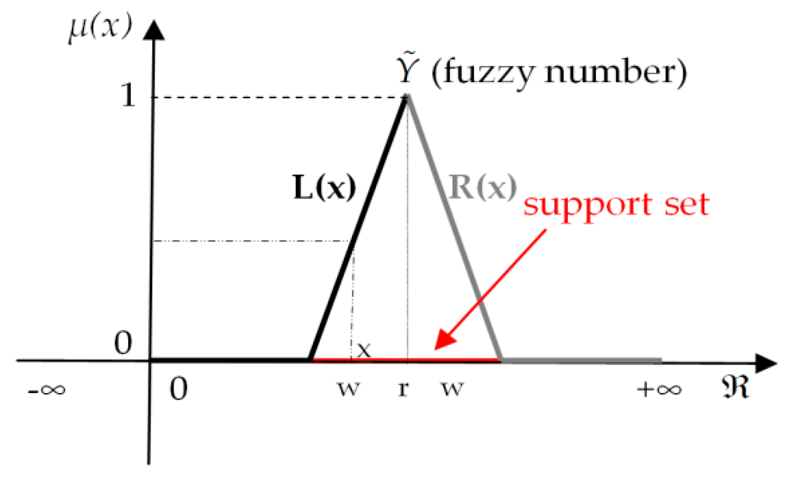
2.1. Basic Consepts of Fuzzy Logic and Sets
- such that (normal fuzzy set)
- the α-cut, , must be a closed interval
- the support set (strong zero-cut), , of the fuzzy number must be bounded
2.2. Fuzzy Linear Regression Analysis
2.2.1. Fuzzy Multiple Linear Regression based on Tanaka’s Model
2.2.2. Modification of Tanaka’s Model with the Use of a Non-linear Objective Function
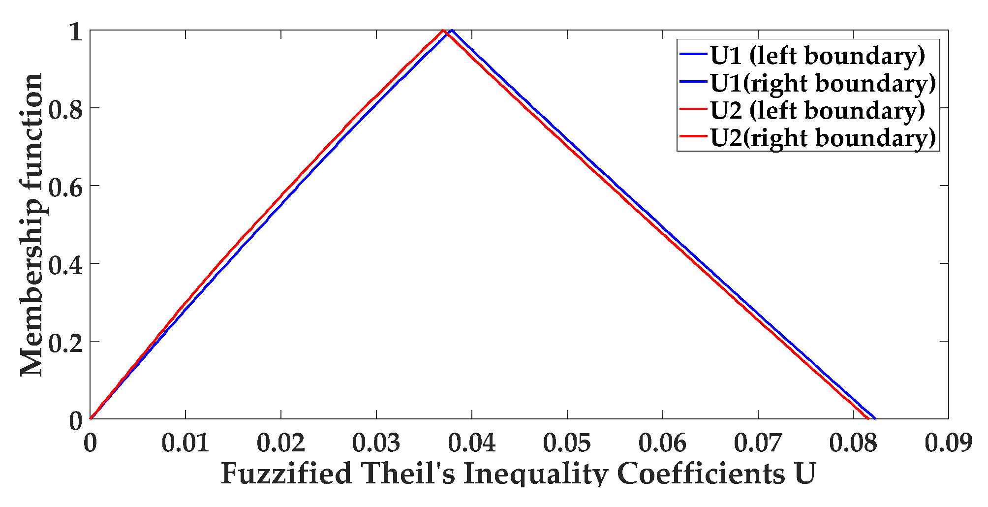
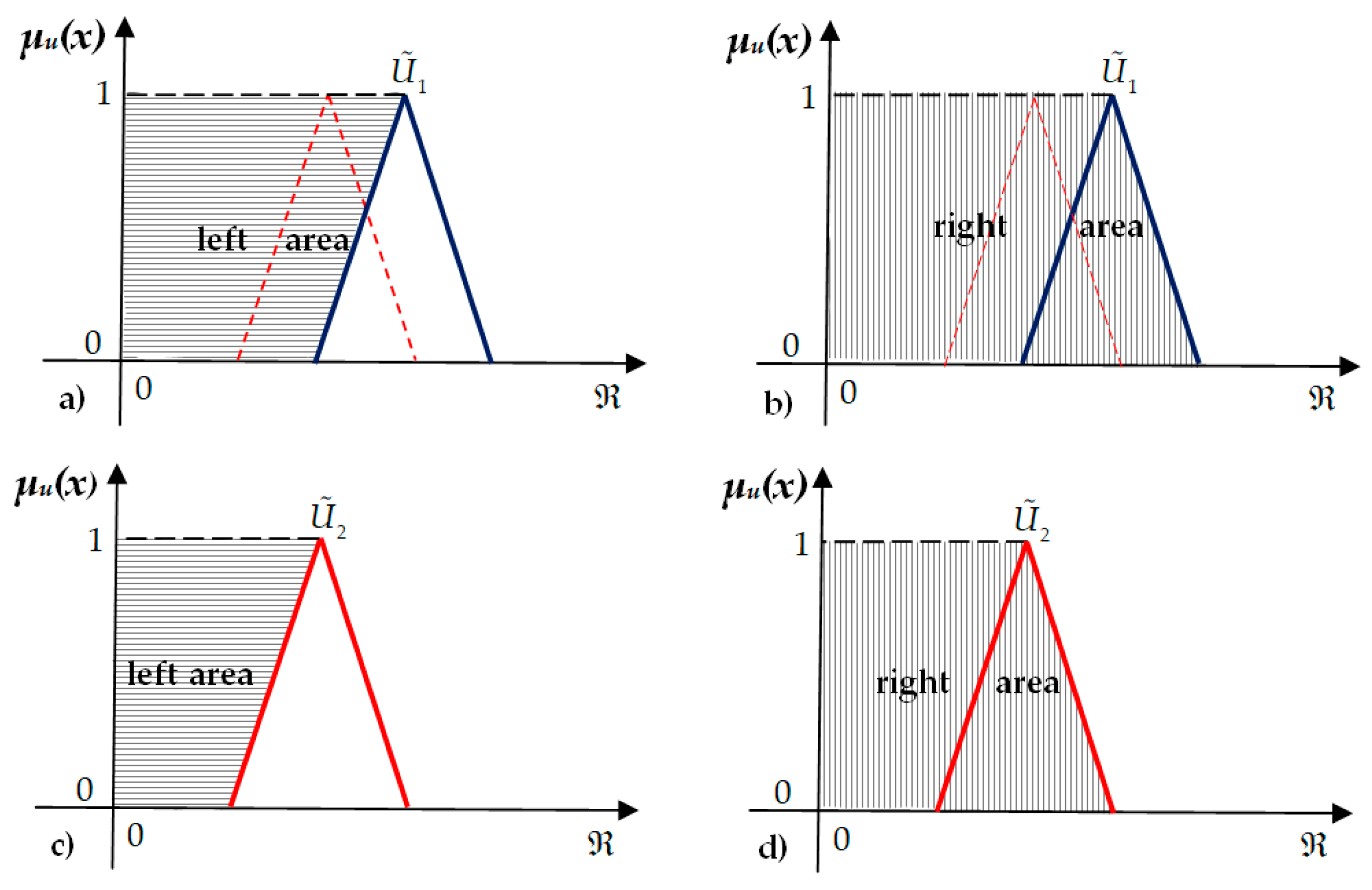
2.3. Suitability Measures
3. Results
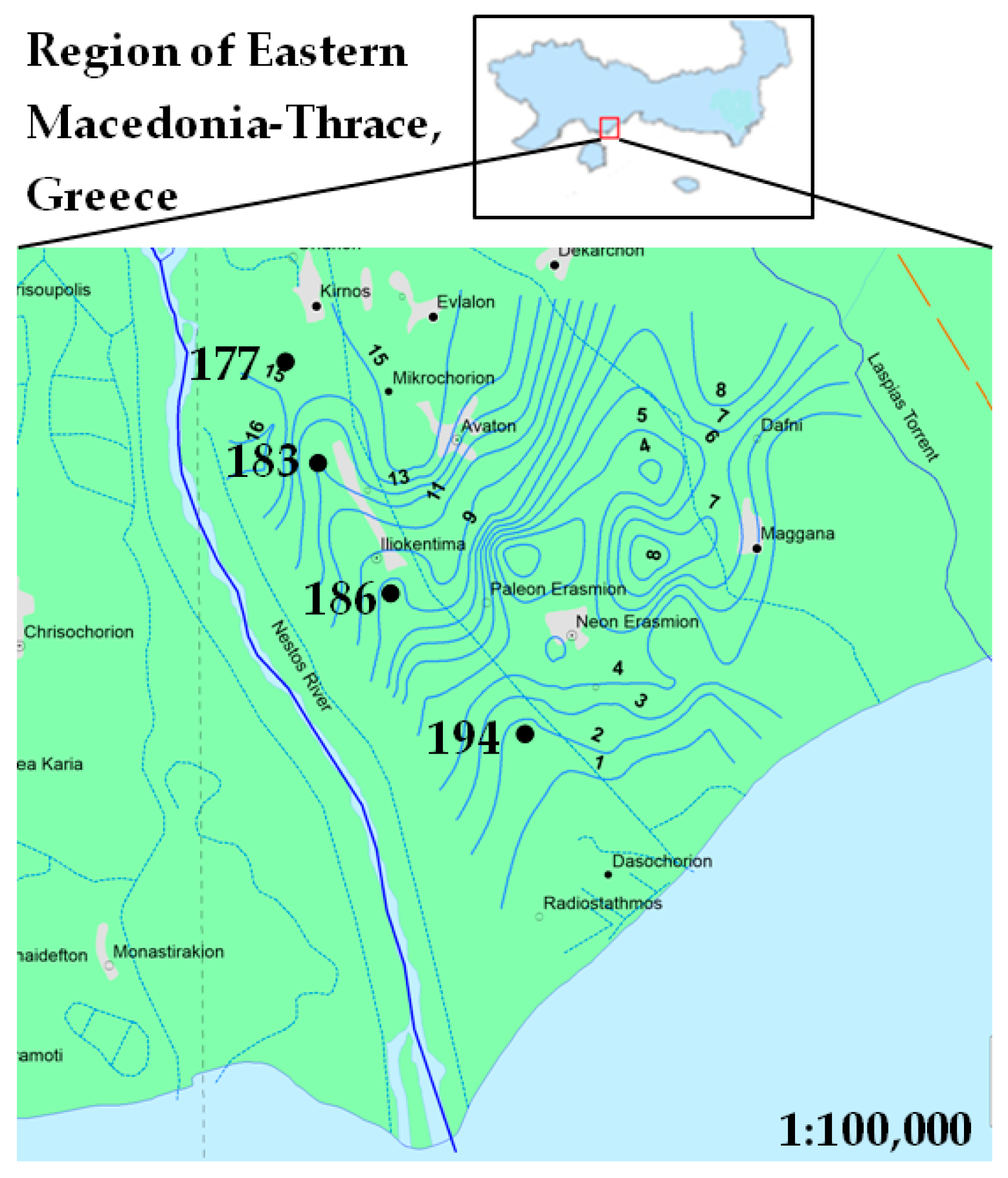
3.1. Case Study
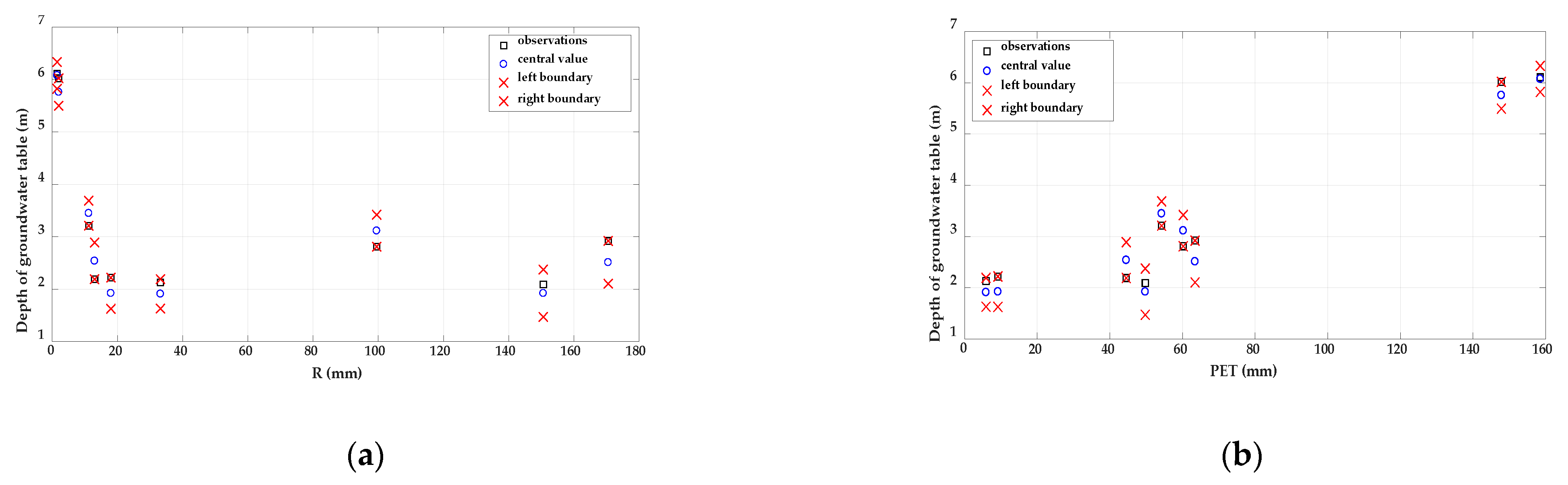
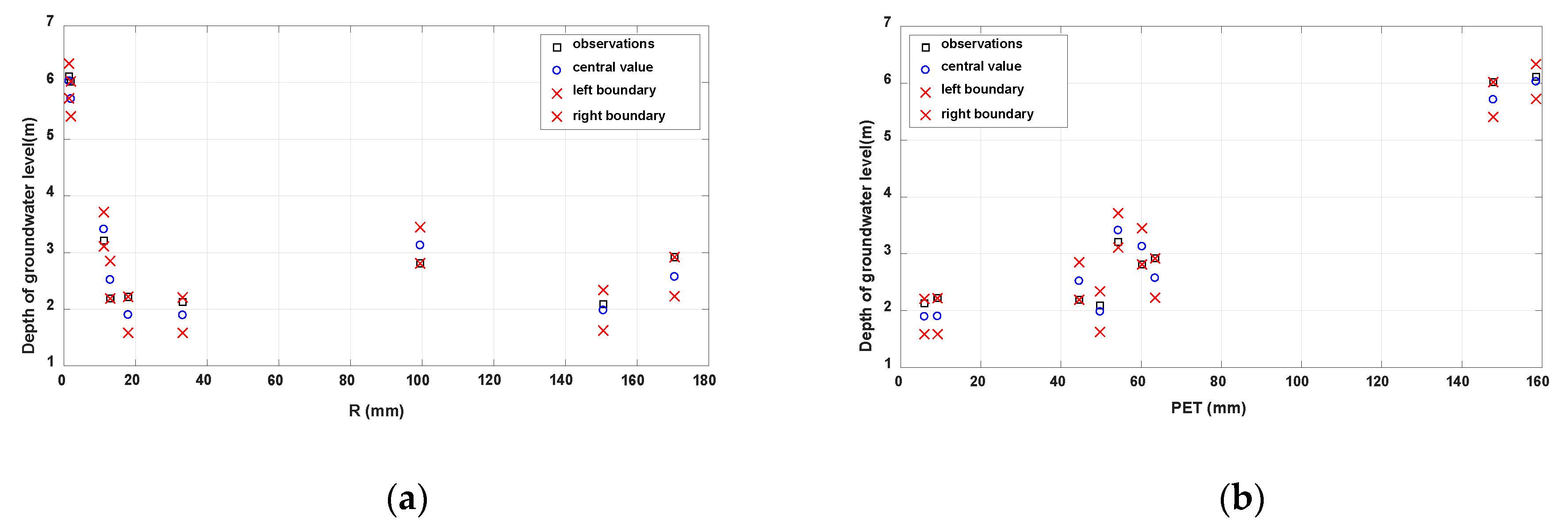
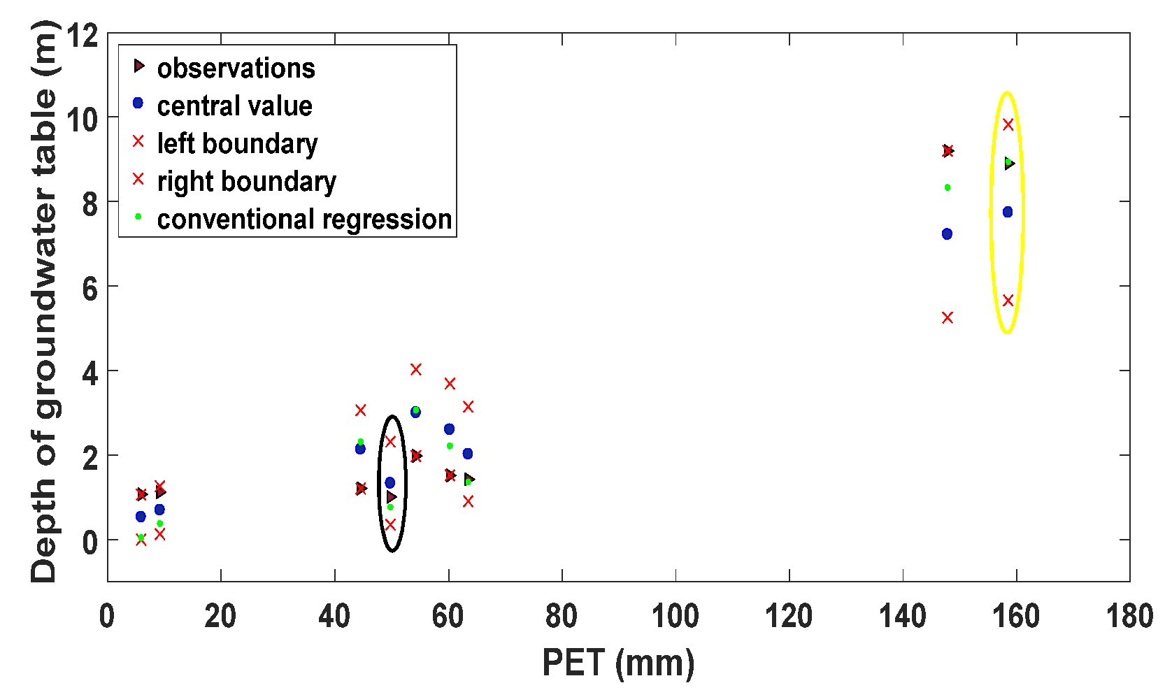
3.2. Results of the Two Fuzzy Regression Models
4. Discussion Points
5. Concluding Remarks
Author Contributions
Funding
Data Availability Statement
Conflicts of Interest
Appendix A

References
- Changnon, S.A.; Huff, F.A.; Hsu, C.-F. Relations between Precipitation and Shallow Groundwater in Illinois. J. Clim. 1988, 1, 1239–1250. [Google Scholar] [CrossRef] [Green Version]
- Zektser, I.; Loaiciga, H.A. Groundwater fluxes in the global hydrologic cycle: Past, present and future. J. Hydrol. 1993, 144, 405–427. [Google Scholar] [CrossRef]
- Apaydin, A. Response of groundwater to climate variation: Fluctuations of groundwater level and well yields in the Halacli aquifer (Cankiri, Turkey). Environ. Monit. Assess. 2009, 165, 653–663. [Google Scholar] [CrossRef] [PubMed]
- Viswanathan, M. Recharge characteristics of an unconfined aquifer from the rainfall-water table relationship. J. Hydrol. 1984, 70, 233–250. [Google Scholar] [CrossRef]
- Ferdowsian, R.; Pannel, D.J.; Mcrron, C.; Ryder, A.; Crossing, L. Explaining groundwater hydrographs: Separating atypical rainfall events from time trends. Aust. J. Soil Res. 2001, 39, 861–875. [Google Scholar] [CrossRef] [Green Version]
- Chen, Z.; E Grasby, S.; Osadetz, K.G. Predicting average annual groundwater levels from climatic variables: An empirical model. J. Hydrol. 2002, 260, 102–117. [Google Scholar] [CrossRef]
- Putthividhya, A.; Jirasirilak, S.; Amto, A.; Petra, S. Prediction of groundwater table depth using direct rainfall-groundwater statistical correlations in Thailand. Suranaree J. Sci. Technol. 2017, 25, 27–36. [Google Scholar]
- Zhang, M.; Singh, H.V.; Migliaccio, K.W.; Kisekka, I. Evaluating water table response to rainfall events in a shallow aquifer and canal system. Hydrol. Process. 2017, 31, 3907–3919. [Google Scholar] [CrossRef]
- Yan, S.; Yu, S.; Wu, Y.; Pan, D.; Dong, J. Understanding groundwater table using a statistical model. Water Sci. Eng. 2018, 11, 1–7. [Google Scholar] [CrossRef]
- Spiliotis, M.; Kitsikoudis, V.; Kirca, V.O.; Hrissanthou, V. Fuzzy threshold for the initiation of sediment motion. Appl. Soft Comput. 2018, 72, 312–320. [Google Scholar] [CrossRef]
- Coppola, E.A.; Duckstein, L.; Davis, D. Fuzzy Rule-based Methodology for Estimating Monthly Groundwater Recharge in a Temperate Watershed. J. Hydrol. Eng. 2002, 7, 326–335. [Google Scholar] [CrossRef]
- Dahiya, S.; Singh, B.; Gaur, S.; Garg, V.K.; Kushwaha, H. Analysis of groundwater quality using fuzzy synthetic evaluation. J. Hazard. Mater. 2007, 147, 938–946. [Google Scholar] [CrossRef] [PubMed]
- Priya, K.L. A fuzzy Logic Approach for Irrigation Water Quality Assessment: A Case Study of Karunya Watershed, India. J. Hydrgeol. Hydrol. Eng. 2013, 2, 1. [Google Scholar]
- Young, C.-C.; Liu, W.-C.; Chung, C.-E. Genetic algorithm and fuzzy neural networks combined with the hydrological modeling system for forecasting watershed runoff discharge. Neural Comput. Appl. 2015, 26, 1631–1643. [Google Scholar] [CrossRef]
- Kim, Y.; Chung, E.-S.; Jun, S.-M.; Kim, S.U. Prioritizing the best sites for treated wastewater instream use in an urban watershed using fuzzy TOPSIS. Resour. Conserv. Recycl. 2013, 73, 23–32. [Google Scholar] [CrossRef]
- Mohamed, M.M.; Elmahdy, S.I. Fuzzy logic and multi-criteria methods for groundwater potentiality mapping at Al Fo’ah area, the United Arab Emirates (UAE): An intergrated approach. Geocarto Int. 2017, 32, 1120–1138. [Google Scholar] [CrossRef]
- Wang, H.; Cai, Y.; Tan, Q.; Zeng, Y. Evaluation of Groundwater Remediation Technologies Based on Fuzzy Multi-Criteria Decision Analysis Approaches. Water 2017, 9, 443. [Google Scholar] [CrossRef] [Green Version]
- Spiliotis, M.; Iglesias, A.; Garrote, L. A multicriteria fuzzy pattern recognition approach for assessing the vulnerability to drought: Mediterranean region. Evol. Syst. 2020, 76, 1–14. [Google Scholar] [CrossRef]
- Bárdossy, A.; Bogardi, I.; Duckstein, L. Fuzzy regression in hydrology. Water Resour. Res. 1990, 26, 1497–1508. [Google Scholar] [CrossRef]
- Guan, J.; Aral, M.M. Optimal design of groundwater remediation systems using fuzzy set theory. Water Resour. Res. 2004, 40. [Google Scholar] [CrossRef] [Green Version]
- Tsakiris, G.; Tigkas, D.; Spiliotis, M. Assessment of interconnection between two using deterministic and fuzzy approaches. Eur. Water 2006, 15, 15–22. [Google Scholar]
- Mathon, B.R.; Ozbek, M.M.; Pinder, G.F. Transmissivity and storage coefficient estimation by coupling the Cooper–Jacob method and modified fuzzy least-squares regression. J. Hydrol. 2008, 353, 267–274. [Google Scholar] [CrossRef]
- Shrestha, R.R.; Simonovic, S.P. Fuzzy Nonlinear Regression Approach to Stage-Discharge Analyses: Case Study. J. Hydrol. Eng. 2010, 15, 49–56. [Google Scholar] [CrossRef]
- Yang, A.L.; Huang, G.H.; Fan, Y.R.; Zhang, X.D. A Fuzzy Simulation-Based Optimization Approach for Groundwater Re-mediation Design at Contaminated Aquifers. Math. Probl. Eng. 2012, 2012, 13. [Google Scholar] [CrossRef]
- Hernandez, E.A.; Hernandez, E.A.; Estrada, F. A multidimensional fuzzy least-squares regression approach for estimating hydraulic gradients in unconfined aquifer formations and its application to the Gulf Coast aquifer in Goliad County, Texas. Environ. Earth Sci. 2013, 71, 2641–2651. [Google Scholar] [CrossRef]
- Chachi, J.; Taheri, S.; Arghami, N. A hybrid fuzzy regression model and its application in hydrology engineering. Appl. Soft Comput. 2014, 25, 149–158. [Google Scholar] [CrossRef]
- Khan, U.T.; Valeo, C. A new fuzzy linear regression approach for dissolved oxygen prediction. Hydrol. Sci. J. 2015, 60, 1096–1119. [Google Scholar] [CrossRef]
- Tzimopoulos, C.; Papadopoulos, K.; Papadopoulos, B. Fuzzy Regression with Applications in Hydrology. Int. J. Eng. Innov. Technol. 2016, 5, 22. [Google Scholar]
- Evangelides, C.; Arampatzis, G.; Tzimopoulos, C. Fuzzy logic regression analysis for groundwater quality characteristics. Desalinat. Water Treat. 2017, 95, 45–50. [Google Scholar] [CrossRef] [Green Version]
- Spiliotis, M.; Kitsikoudis, V.; Hrissanthou, V. Assessment of bedload transport ingravel-bed rivers with a new fuzzy adaptive regression. Eur. Water 2017, 57, 237–244. [Google Scholar]
- Tzimopoulos, C.; Evangelides, C.; Vrekos, C.; Samarinas, N. Fuzzy Linear Regression of Rainfall-Altitude Relationship. Proceedings 2018, 2, 636. [Google Scholar] [CrossRef] [Green Version]
- Bárdossy, A.; Mascellani, G.; Franchini, M. Fuzzy unit hydrograph. Water Resour. Res. 2006, 42, 02401. [Google Scholar] [CrossRef] [Green Version]
- Tzimopoulos, C.; Papadopoulos, K.; Papadopoulos, B.K. Models of Fuzzy Linear Regression: An Application in Engineering. In Springer Optimization and Its Applications; Springer Nature: New York, NY, USA, 2016; Volume 111, pp. 693–713. [Google Scholar]
- Tayfur, G.; Brocca, L. Fuzzy Logic for Rainfall-Runoff Modelling Considering Soil Moisture. Water Resour. Manag. 2015, 29, 3519–3533. [Google Scholar] [CrossRef] [Green Version]
- Klir, G.J.; Yuan, B. Fuzzy Sets and Fuzzy Logic. Theory and Applications; Prentice Hall: Upper Saddle River, NJ, USA, 1995. [Google Scholar]
- Hanss, M. Applied Fuzzy Arithmetic, an Introduction with Engineering Applications; Springer: Berlin/Heidelberg, Germany, 2005. [Google Scholar]
- Ross, T.J. Fuzzy Logic with Engineering Applications, 4th ed.; Wiley: Hoboken, NJ, USA, 2010. [Google Scholar]
- Saridakis, M.; Spiliotis, M.; Angelidis, P.B.; Papadopoulos, B.K. Assessment of the Couple between the Historical Sample and the Theoretical Probability Distributions for Maximum flow Values Based on a Fuzzy Methodology. Environ. Sci. Proc. 2020, 2, 22. [Google Scholar] [CrossRef]
- Buckley, J.J.; Eslami, E.; Feuring, T. Fuzzy Mathematics in Economics and Engineering; Springer Nature: New York, NY, USA, 2002; p. 272. [Google Scholar]
- Tanaka, H. Fuzzy data analysis by possibilistic linear models. Fuzzy Sets Syst. 1987, 24, 363–375. [Google Scholar] [CrossRef]
- Papadopoulos, B.K.; Sirpi, M.A. Similarities in Fuzzy Regression Models. J. Optim. Theory Appl. 1999, 102, 373–383. [Google Scholar] [CrossRef]
- Profillidis, V.A.; Papadopoulos, B.K.; Botzoris, G.N. Similarities in fuzzy regression models and application on transportation. Fuzzy Econ. Rev. 1999, 4, 83–98. [Google Scholar] [CrossRef]
- Spiliotis, M.; Papadopoulos, C.; Angelidis, P.B.; Papadopoulos, B.K. Hybrid Fuzzy—Probabilistic Analysis and Classification of the Hydrological Drought. Proceedings 2018, 2, 643. [Google Scholar] [CrossRef] [Green Version]
- Diamond, P. Fuzzy least squares. Inf. Sci. 1988, 46, 141–157. [Google Scholar] [CrossRef]
- Papadopoulos, C.; Spiliotis, M.; Angelidis, P.; Papadopoulos, B. A hybrid fuzzy frequency factor based methodology for analyzing the hydrological drought. Desalinat. Water Treat. 2019, 167, 385–397. [Google Scholar] [CrossRef]
- Ubale, A.B.; Sananse, S.L. A comparative study of fuzzy multiple regression model and least square method. Int. J. Appl. Res. 2016, 2, 11–15. [Google Scholar]
- Theil, H. Applied Economic Forecasting; North-Holland Publishing Company: Amsterdam, The Netherlands, 1966. [Google Scholar]
- Bliemel, F. Theil’s Forecast Accuracy Coefficient: A Clarification. J. Mark. Assoc. 1973, 10, 444–446. [Google Scholar]
- Botzoris, G.; Papadopoulos, B. Fuzzy Sets: Applications on the Design and the Management of Engineering Projects; Sofia Publishing: Thessaloniki, Greece, 2015; p. 402. (In Greek) [Google Scholar]
- Mwila, G. Groundwater Quality Degradation Due to Seawater Intrusion Conditions in a Coastal Unconfined Aquifer in Northern Greece. Master’s Thesis, Institute of Applied Geosciences, Tropical Hydrogeology, Engineering Geology and Environmental Management (MSc-Trophee), Technical University of Darmstadt, Darmstadt, Germany, 2009. [Google Scholar]
- Gkiougkis, I. Investigation of the Qualitative Degradation of the Groundwater Aquifer System of the Eastern Delta of the River Nestos. Master’s Thesis, Hellenic Open University, Patra, Greece, 2010. [Google Scholar]
- Gkiougkis, I. Seawater Intrusion Assessment in Coastal Aquifers in a Deltaic Environment: The Case of Nestos RiverDelta. Ph.D. Thesis, Department of Civil Engineering, D.U.Th., Xanthi, Greece, 2018. [Google Scholar]
- Sakkas, I.; Diamantis, I.; Pliakas, F. Groundwater Artificial Recharge Study of Xanthi-Rhodope Aquifers (in Thrace, Greece); Greek Ministry of Agriculture Research Project, Final Report; Sections of Geotechnical Engineering and Hydraulics of the Civil Engineering Department of Democritus University of Thrace: Xanthi, Greece, 1998. (In Greek) [Google Scholar]
- Pliakas, F.; Diamantis, I.; Petalas, C. Saline water intrusion and groundwater artificial recharge in east delta of Nestos River. In Proceedings of the 7th International Conference on Environmental Science and Technology, University of the Aegean, Ermoupolis, Syros, Greece, 3–6 September 2001; Department of Environmental Studies and Global Nest: Budapest, Hungary, 2011; Volume 2, pp. 719–726. [Google Scholar]
- Nguyen, T.-L. Methods in Ranking Fuzzy Numbers: A Unified Index and Comparative Reviews. Complexity 2017, 2017, 1–13. [Google Scholar] [CrossRef]


| Wells | Constant Term | R | PET | Qmean | ||||
|---|---|---|---|---|---|---|---|---|
(centre) | (semi-width) | (centre) | (width) | (centre) | (width) | (centre) | (width) | |
| 177 | 0.7371 | 0.4752 | −0.0048 | 0 | 0.0456 | 0.0101 | −0.0281 | 0 |
| 183 | 1.4440 | 0.6340 | −0.0044 | 0 | 0.0416 | 0 | −0.0384 | 0 |
| 186 | 1.2953 | 0.6977 | −0.0021 | 0 | 0.0403 | 0 | −0.0334 | 0 |
| 194 | 2.2853 | 0.1977 | −0.0011 | 0 | 0.0260 | 0 | −0.0442 | 0.0075 |
| Wells | Constant Term | R | PET | Qmean | ||||
|---|---|---|---|---|---|---|---|---|
(centre) | (semi-width) | (centre) | (width) | (centre) | (width) | (centre) | (width) | |
| 177 | 0.7790 | 0.4743 | −0.0059 | 0 | 0.0452 | 0.0103 | −0.0283 | 0 |
| 183 | 1.4824 | 0.6416 | −0.0058 | 0 | 0.0413 | 0 | −0.0384 | 0 |
| 186 | 1.3093 | 0.7005 | −0.0026 | 0 | 0.0402 | 0 | −0.0334 | 0 |
| 194 | 2.2438 | 0.2914 | −0.0007 | 0 | 0.0259 | 0 | −0.0432 | 0.0020 |
| Results based on the FLR-1 model | ||||||
| Wells | J | S | LU | CU | RU | Edis |
| 177 | 10.294 | 46.779 | 0.000 | 0.1212 | 0.2803 | 0.800 |
| 183 | 5.706 | 12.348 | 0.000 | 0.0653 | 0.1401 | 0.905 |
| 186 | 6.279 | 14.293 | 0.000 | 0.0700 | 0.1498 | 0.874 |
| 194 | 2.847 | 3.229 | 0.000 | 0.0379 | 0.0823 | 0.937 |
| Results based on the FLR-2 model | ||||||
| Wells | J | S | UL | UC | UR | Edis |
| 177 | 10.371 | 46.650 | 0.000 | 0.1196 | 0.2801 | 0.802 |
| 183 | 5.774 | 12.175 | 0.000 | 0.0633 | 0.1397 | 0.908 |
| 186 | 6.304 | 14.272 | 0.000 | 0.0695 | 0.1509 | 0.875 |
| 194 | 2.899 | 3.154 | 0.000 | 0.0370 | 0.0816 | 0.939 |
| Ranking Measure/Wells | 177 | 183 | 186 | 194 |
|---|---|---|---|---|
| R (for ) | 0.1277 | 0.0669 | 0.0717 | 0.0391 |
| R (for ) | 0.1266 | 0.0652 | 0.0717 | 0.0384 |
Publisher’s Note: MDPI stays neutral with regard to jurisdictional claims in published maps and institutional affiliations. |
© 2021 by the authors. Licensee MDPI, Basel, Switzerland. This article is an open access article distributed under the terms and conditions of the Creative Commons Attribution (CC BY) license (http://creativecommons.org/licenses/by/4.0/).
Share and Cite
Papadopoulos, C.; Spiliotis, M.; Gkiougkis, I.; Pliakas, F.; Papadopoulos, B. Relating Hydro-Meteorological Variables to Water Table in an Unconfined Aquifer via Fuzzy Linear Regression. Environments 2021, 8, 9. https://0-doi-org.brum.beds.ac.uk/10.3390/environments8020009
Papadopoulos C, Spiliotis M, Gkiougkis I, Pliakas F, Papadopoulos B. Relating Hydro-Meteorological Variables to Water Table in an Unconfined Aquifer via Fuzzy Linear Regression. Environments. 2021; 8(2):9. https://0-doi-org.brum.beds.ac.uk/10.3390/environments8020009
Chicago/Turabian StylePapadopoulos, Christopher, Mike Spiliotis, Ioannis Gkiougkis, Fotios Pliakas, and Basil Papadopoulos. 2021. "Relating Hydro-Meteorological Variables to Water Table in an Unconfined Aquifer via Fuzzy Linear Regression" Environments 8, no. 2: 9. https://0-doi-org.brum.beds.ac.uk/10.3390/environments8020009