Article

Performance Evaluation of Two Machine Learning Techniques in Heating and Cooling Loads Forecasting of Residential Buildings

by
Arash Moradzadeh
1,
Amin Mansour-Saatloo
1,
Behnam Mohammadi-Ivatloo
1,2,* and
Amjad Anvari-Moghaddam
1,3,*
1
Faculty of Electrical and Computer Engineering, University of Tabriz, Tabriz 5166616471, Iran
2
Institute of Research and Development, Duy Tan University, Da Nang 550000, Vietnam
3
Department of Energy Technology, Aalborg University, 9220 Aalborg, Denmark
*
Authors to whom correspondence should be addressed.
Submission received: 29 April 2020 / Revised: 23 May 2020 / Accepted: 29 May 2020 / Published: 31 May 2020
(This article belongs to the Special Issue Renewable Energy Systems 2020)

Abstract

:
Nowadays, since energy management of buildings contributes to the operation cost, many efforts are made to optimize the energy consumption of buildings. In addition, the most consumed energy in the buildings is assigned to the indoor heating and cooling comforts. In this regard, this paper proposes a heating and cooling load forecasting methodology, which by taking this methodology into the account energy consumption of the buildings can be optimized. Multilayer perceptron (MLP) and support vector regression (SVR) for the heating and cooling load forecasting of residential buildings are employed. MLP and SVR are the applications of artificial neural networks and machine learning, respectively. These methods commonly are used for modeling and regression and produce a linear mapping between input and output variables. Proposed methods are taught using training data pertaining to the characteristics of each sample in the dataset. To apply the proposed methods, a simulated dataset will be used, in which the technical parameters of the building are used as input variables and heating and cooling loads are selected as output variables for each network. Finally, the simulation and numerical results illustrates the effectiveness of the proposed methodologies.

1. Introduction

Increasing the number of cities and their populations throughout the world requires a great deal of energy to meet the needs of citizens. Recent studies have predicted that the population of cities will increase up to five billion by 2030 [1]. Nearly 40% of total energy consumption is related to the dwellings, and other building types constitute just a fraction of the buildings [2]. Supplying energy to the citizens requires associated resources in which limited sources are available. As the consumption of residential buildings forms a great amount of demand, regarding social welfare, residential consumption should be monitored and controlled [3]. On the other hand, heating and cooling are the most crucial energy sources among citizens, so in this regard usage of these energies should be managed.
Managing and optimizing the energy consumption of buildings requires having complete information about the performance of the building and environmental factors. Electricity, gas and heating supply are the most important resources of energy in a building, but the important final use applications are elevators, heating ventilation and air conditioning (HVAC), domestic hot water, and so on. Among the aforementioned energy sources, optimal operation of HVAC and indoor condition supply are two important factors in evaluating building energy performance [4,5]. HVAC, as a basic infrastructure in the building, plays an important role by changing the amount of internal cooling and heating loads of residential buildings. Despite the need for this system in buildings, there is a major concern that about 40% of all energy, especially in office buildings, is consumed by this system [6,7]. Forecasting the thermal loads plays an important role in optimizing the cooling and heating cost of the buildings, as the deviation from the optimally scheduled values will increase the total cost considerably [8].
Energy forecasting is a way to reach optimal operation of HVAC and energy management of residential buildings. In this regard, residential buildings’ consumption patterns could be predicted [9]. Nowadays, by developing technology many small-scale smart devices and building management systems (BMSs) can be installed on the residential buildings sites in order to monitor and record the load patterns of the buildings, and also environmental characteristics that have a high impact on the energy forecasting. Using such data, building consumption patterns could be predicted and controlled hourly. In addition, the necessity of energy forecasting has been expressed by some researches e.g., a review study of thermal energy consumption in the buildings pertinent to the comfort was introduced in [10] and the purpose of the study was showing how social-economic, fuel mix and climate change are affected by thermal energy comfort. Moreover, by load forecasting, buildings can schedule for the next day, not only to participate in the demand–response programs [11,12,13] but also to participate in energy trading [14,15].
So far, many studies have been done in order to evaluate load forecasting of the buildings. In a valuable study [16], an integrated design approach has been utilized to estimate life-cycle energy savings, cost-effectiveness of energy efficiency measures in new buildings, and carbon emission reduction. In [17], a multi-objective optimization for energy refurbishments of existing buildings through energy efficiency measures and HVAC systems have been carried out using a genetic algorithm coupled with a dynamic simulation tool. Predictor methods for heating load based on artificial neural networks (ANN) have been evaluated in [18] for office buildings where the impact of data size and dimensionality in ANN was inspected. In order for heating, ventilation, and air-conditioning (HVAC) system optimization in [19], electricity load forecasting based on ANN has been studied. Among three utilized algorithms such as Levenberg-Marquardt, Scaled Conjugate gradient back-propagation, and Bayesian Regularization (BR), the BR-based ANN showed the best performance. Another study proposed the energy forecasting method using statistical analysis for heating and cooling of an office building [20]. In [21], four hybrid techniques based on artificial neural network (ANN) and meta-heuristic algorithms such as artificial bee colony (ABC) optimization, particle swarm optimization (PSO), imperialist competitive algorithm (ICA), and genetic algorithm (GA) have been suggested for forecasting the heating load of buildings’ energy efficiency. Forecasting the cooling load has been done in [22] using a probabilistic entropy-based neural (PENN) method. Short-term cooling load prediction in order to optimize the operation of HVAC systems and energy efficiency measures in buildings has been done in [23] using multiple nonlinear regression (MNR), auto regressive (AR), and autoregressive with exogenous (ARX) models. In [24], the thermal comfort reduction of the energy consumption in the building by 36.5% was performed via a feedforward neural network (FFNN). A decision tree method has been suggested in [25] for energy demand forecasting and energy efficiency measures of a residential building. A comparative study of forecasting methods for heating and cooling load was done in [26], where machine learning techniques such as a deep neural network (DNN), gradient boosted machine (GBM), Gaussian process regression (GPR) and minimax probability machine regression (MPMR) were compared with each other. In [27], prediction of the cooling and heating loads of the building were done using ANN, classification and regression tree (CART), general linear regression (GLR), and chi-squared automatic interaction detector (CHAID). In the same work, the technical characteristics of the building were considered as input to the networks. In [28], sixteen residential buildings were evaluated in terms of heating and cooling energy consumption forecasting via adaptive linear time-series models. Likewise, cooling load forecasting based on data mining techniques was proposed in [29] to help design a more efficient building management system (BMS). In [30], the BMS based on electrical, economic, and ecological optimization using a genetic algorithm was introduced to improve energy efficiency of the buildings. General regression neural network (GRNN) has also been employed in [31] for cooling energy forecasting to optimize HVAC heat storage of public buildings.
In most of the aforementioned research works, meteorological data was used as an indicator and input for forecasting the cooling and heating loads of residential buildings. It is undeniable that environmental and meteorological factors do not affect the cooling and heating loads of residential buildings, but sometimes abrupt changes in weather could disrupt energy forecasting equations, reducing the accuracy coefficient and increasing the error in the energy forecasting operation. In this paper, high-precision prediction of cooling and heating loads of a building was done by using multilayer perceptron (MLP) and support vector regression (SVR) methods. A set of data on structural characteristics of the building was considered as an input variable, while the amount of cooling and heating load was considered as an output variable. Using this data and creating a linear mapping between input and output variables via the proposed methods, it is possible to make a more accurate prediction of cooling and heating loads.
The rest of the paper is organized as follows: Section 2 describes the case study and dataset. Section 3 represents the employed methodologies and techniques. Section 4 includes the simulation and numerical results and finally, Section 5 concludes the paper.

2. Case Study

The dataset used in this work was created by Tsanas and Xifara [32]. Twelve different buildings were simulated in Ecotect software to generate the dataset. The glazing area, distribution of the glazing area and the orientation are the parameters that make the buildings different from each other. Each building was simulated using eighteen preliminary cubes (3.5 × 3.5 × 3.5 m3) with the same materials for all buildings. The newest and most common materials in the building construction industry were selected for each of the eighteen elements so that the materials used for each of these elements were the same for all forms of construction. In the design process, three types of glazing areas such as 10%, 25%, and 40% were used as percentages of the floor area. In addition, it was assumed that buildings were in Greece, Athens. Sixty percent humidity, 0.3 m/s wind speed, lightning level of 300 1 x and 0.6 clo of clothing were considered as internal design conditions during simulation, while the infiltration rate was set to 0.5 for the air change rate with a wind sensitivity of 0.25 air changer per hour. The dataset includes 768 samples with eight features for each sample, namely x 1 , x 2 , , x 8 and y 1 , y 2 as decision variables, which are listed in Table 1 [21,32]. This work aims to forecast y 1 as the heating load and y 2 as the cooling load using the aforementioned features as decision variables. Although the dataset was generated via simulation, it is notable that the proposed methods are applicable to the real-world dataset.

3. Methods

Artificial neural network (ANN) and machine learning algorithms as powerful tools in data mining were employed to do the modelling and forecasting tasks [33,34]. In this work, MLP and SVR were used as two application models of these algorithms to create a linear mapping between the technical parameters of building and the cooling and heating loads of the building in order to forecast the load/energy. In the following, each of the proposed methods are briefly introduced.

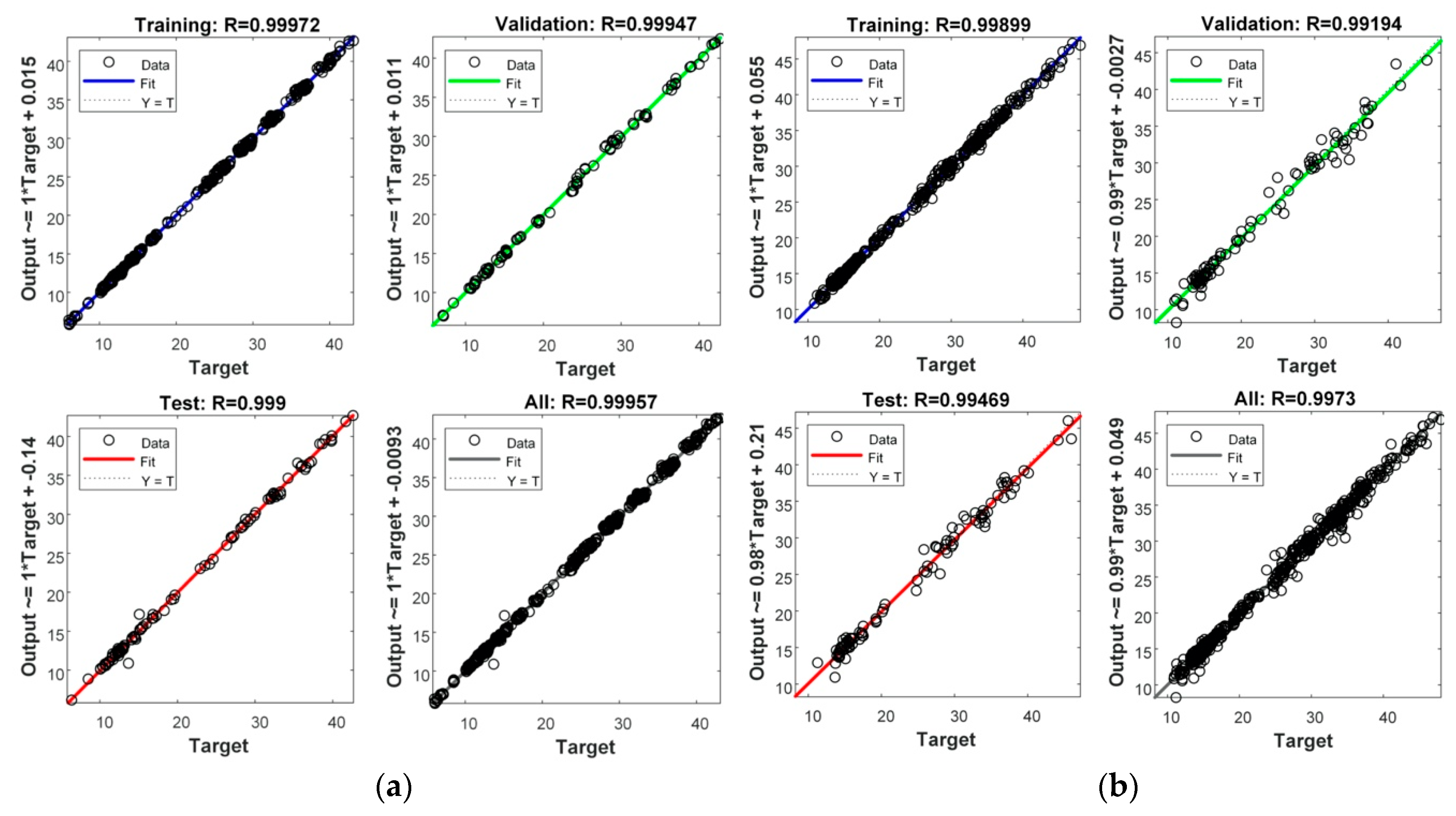
3.1. Multilayer Perceptron (MLP)

MLP has a fully connected layer structure, i.e., each neuron in a layer is connected to all neurons in the next and previous layers. The schematic of the MLP structure is shown in Figure 1, which illustrates a nonlinear mapping between the input vector and the output vector [35]. The neurons are connected through weights, and output signals are generated by a nonlinear transfer function [36].
Y = f ( b + l = 1 N w l x l )
In Equation (1) Y and x are the output and input signals, respectively, f is the nonlinear transfer function, b and w are the bias and weight vectors, respectively, and N is the total number of the inputs. Since MLP has the ability to learn through training, a dataset with known input vector and output vector is required in which the weight vector is adjusted according to the output signals through training [37].

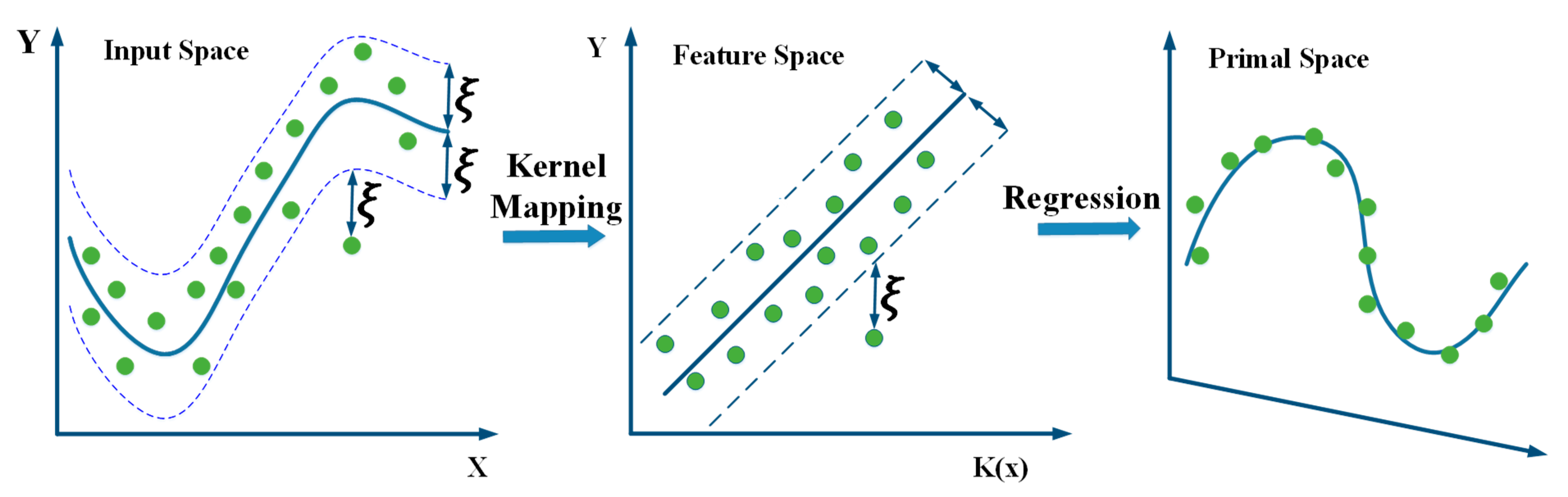
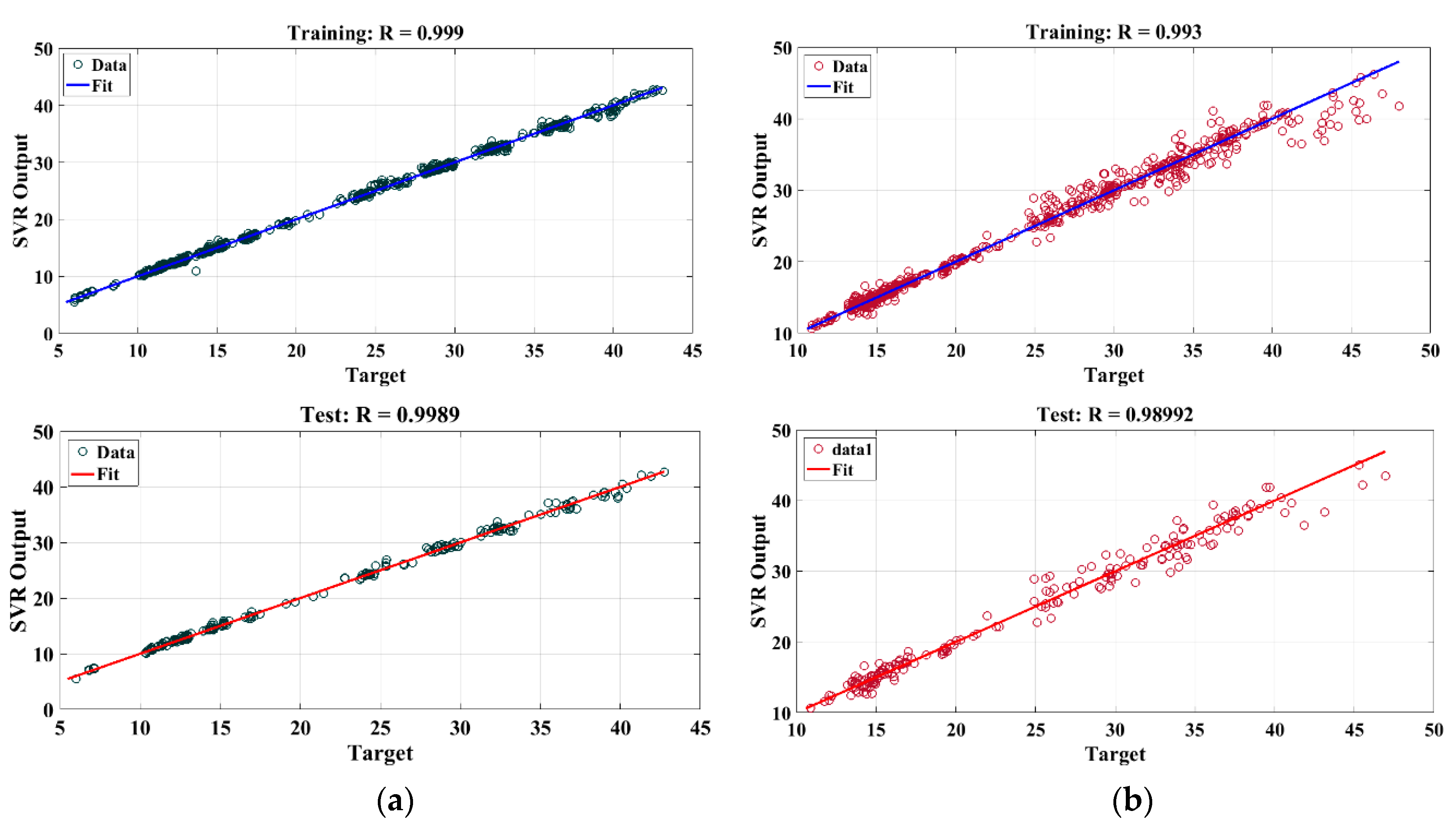
3.2. Support Vector Regression (SVR)

SVR is one of the training tools which was developed from the support vector machine (SVM). The principle of SVR is depicted in Figure 2. In this work, ε-SVR is employed for the training of data. ε-SVR is a classic model of SVR with the aim of finding a flat function, which has a small (ε) error from the obtained target [38]. In the case of SVR, the following function is trained using given training data such as { ( x 1 , y 1 ) , ( x 2 , y 2 ) , , ( x l , y l ) , ( x N , y N ) } χ × R , l = { 1 , 2 , , N } , where χ illustrates the space of the input patterns:
f ( x ) = w , x + b ; w χ , b R
where b is bias, and w , x represents the linear function of fitting input space to the feature space. Equation (3) is using to minimizing the risk function as follows:
R = 1 2 w 2 + c i = 1 N ( y 1 , w , x )
In Equation (3), the selected loss function and c > 0 specifies the tradeoff between the smoothness of f and allowed deviation larger than ε. In order to deal with the problem, the minimization problem of (4) must be solved.
min 1 2 w 2 + c l = 1 N ( ξ l + ξ l * )
s . t . { y l w , x l b ε + ξ l w , x l + b y l ε + ξ l * ξ l + ξ l * 0
where, ξ l , ξ l * are the slack variables which tackle the infeasible constraints. In order to solve the optimization problem, the dual problem of the (4) can be derived using the Lagrange function. In addition, w can be defined as an integration of training patterns of x linearly. Therefore, Equation (2) can be reformulated as [39]:
f ( x ) = b + l = 1 N ( α l α l * ) x l , x
where, α l , α l * are the Lagrangian multipliers. Then, in order to put the nonlinearity in the algorithm, the training patterns x l can be modified by a map Φ : χ F . In addition, Kernel function can be defined as:
k ( x , x ) : = Φ ( x ) , Φ ( x )
According to the above-mentioned equations, the optimization problem of (4) can be modified, and finally, the function f derived as follows:
f ( x ) = b + l = 1 N ( α l α l * ) k ( x l , x )
It is notable that in the nonlinear optimization problem, the flatness function is searched among the feature space, not input space [40,41].

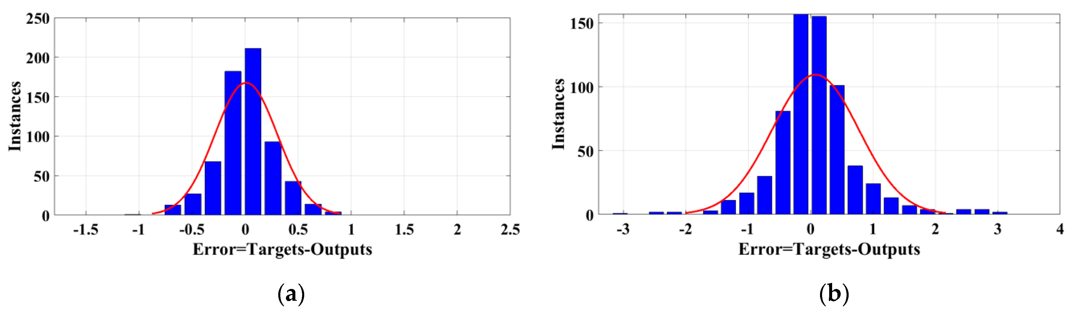
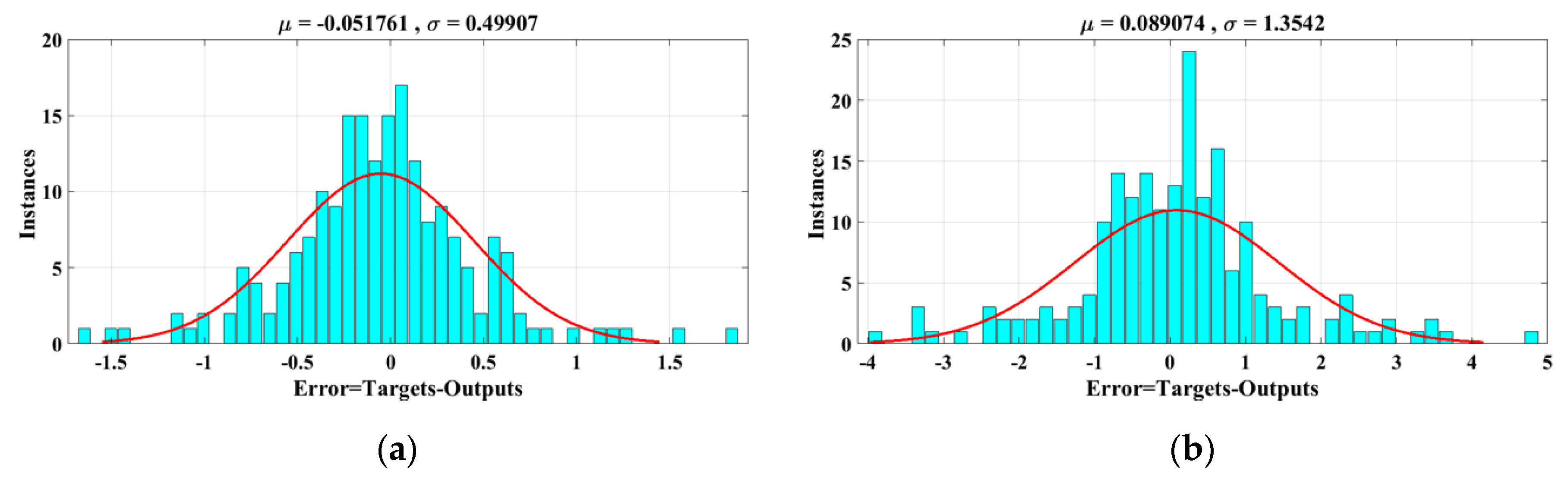
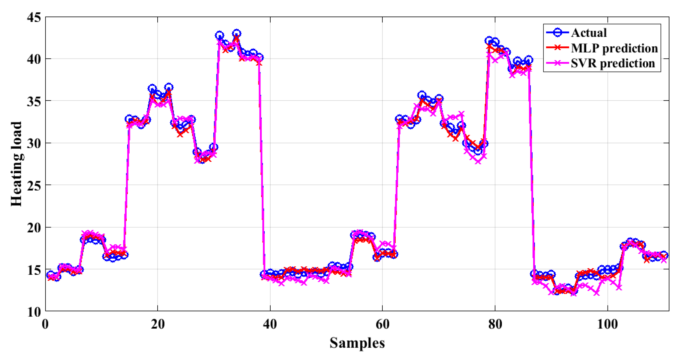
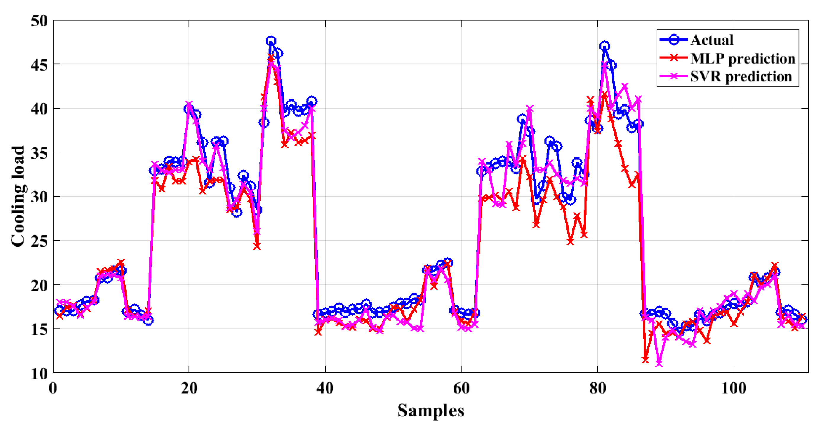
4. Simulation and Results

The MLP and SVR networks are designed to predict the cooling and heating load. Each of these networks was trained using a dataset as input. In this paper, 85% (658 samples) of the data were used to train and validate the proposed methods and the remaining 15% (110 samples) were used for testing. In the first stage, each network required a preliminary design to determine the number of neurons in the hidden layer and the coefficients of the network. After designing each network, the amount of training and testing data for the network was determined. In this work, 70% of the samples were considered as training data and 30% as test data to validate the training phase of each network. After training and testing each neural network or regression algorithm, the results need to be evaluated. To do this, correlation coefficient (R), mean squared error (MSE), root mean squared error (RMSE), and mean absolute error (MAE) can be used as statistical performance metrics. Each of the mentioned indices are calculated according to the following equations [42].
R = l = 1 N ( x l x ¯ ) ( y l y ¯ ) l = 1 N ( x l x ¯ ) 2 l = 1 N ( y l y ¯ ) 2
R M S E = 1 N l = 1 N ( x l y l ) 2
M S E = 1 N l = 1 N ( x l y l ) 2
M A E = 1 N l = 1 N | x l y l |
where x l and y l illustrate the actual value and predicted value. x ¯ and y ¯ y ¯ depict the mean of actual values and forecasted values, respectively. Figure 3 shows the good correlation coefficient between the real values and the predicted value by the network in the training, testing and validation steps for the MLP network. Figure 4 indicates an excellent correlation coefficient between the real values and the predicted value for the SVR network during the training phase.
Given the excellent correlation between the target data and the output of each network (as shown in Figure 3 and Figure 4), it can be clearly understood that each of these networks have passed the training phase well. Good training means that the network is able to identify inherent patterns in the nature of data and to predict the unknown data by using the learned patterns, so that each network learns how much of a cooling and heating load is required for each building with specific characteristics. With this training, each network can predict the amount of cooling and heating loads related to the input data of the test phase. After training, each network is validated using initial test data (30% of 85%). This is kind of a test for the training phase, which is done by the network itself. The prediction error in the test or validation, which is one of the most important values in evaluating the results, is presented in Figure 5 and Figure 6 for each of the MLP and SVR networks in the histogram form, respectively.
The error obtained in the error histogram model indicates the minimum and maximum prediction error. This means that in predicting the cooling and heating loads for the test data, the amount of error that each of the trained networks can have is equal to the amount provided in the above figures.
In evaluating and analyzing each of the above figures that somehow represent the performance of each network in the initial training and testing stages, it can be concluded that the training of proposed methods has been well validated using the desired data. It should be noted that when the network is trained with high accuracy, it is well designed and the amount of error in the validation and initial testing process depends more on the type of data. It also implies that the network will be able to accurately assess and predict new and unknown data. Each network is saved as a black box after training. This black box contains patterns that the network was able to identify during the training phase. Now, the new and unknown data must be used to test these networks and predict the cooling and heating load of buildings. To do this, 15% (110 samples) of the data, kept as unknown and new data, were used. Figure 7 and Figure 8 show the results of forecasting heating and cooling loads for new data using the trained MLP and SVR networks, respectively.
Performance evaluation of the proposed methods is presented in Table 2 in terms of R, MSE, RMSE, and MAE.
Based on the results presented in the Table 2, it can be seen that the best prediction was related to the prediction of the heating load by the MLP method with the highest value of R (0.9993) and minimal errors in the form of MSE (0.2335), RMSE (0.4832), and MAE (0.4118). However, in predicting the cooling load, the SVR method with a large amount of R (0.9878) and lowest errors in the terms of MSE (3.024), RMSE (1.7389), and MAE (1.4762) made a good prediction. Highest values of MSE and RMSE errors of prediction were also related to the MLP method in the prediction of cooling load. The use of machine learning methods and their results are highly dependent on the type of input data. It is observed that there is a difference between the results of predicting the cooling load and heating load by each of the networks and the heating load is predicted with high accuracy. This difference is due to the poor correlation between the input data and the amount of cooling load relative to the heating load. To evaluate the effectiveness of the proposed methods in this paper, it is necessary to compare the results obtained with the results of other studies. Comparisons should be made with caution using similar datasets. To this end, a number of studies were selected for comparison in which similar data was used for predicting the cooling and heating loads. To express the effectiveness of the data type in the accuracy of the results, the results of several studies conducted to predict cooling and heating loads using different data were compared with the results obtained in this paper. Table 3 makes this comparison.
The comparison made in Table 3, shows the accuracy and efficiency of the proposed methods in this paper for forecasting the cooling and heating loads of the building. The use of machine learning applications and the selection of the applicable method for energy predicting and energy efficiency measures in residential buildings are significantly effective in saving energy consumption. The selected methods were able to realize the purpose of the paper with their high accuracy and achieve this important goal. Finally, it should be noted that the proposed solutions can also be used for real-world data.

5. Conclusions

Nowadays, the importance of energy saving and its management has raised many challenges in forecasting the heating and cooling loads of buildings. Most researchers in this field offer many methods and models for predicting heating and cooling loads to somehow increase the prediction accuracy. In this paper, based on machine learning models two MLP and SVR methods were proposed to predict the cooling and heating load of a residential building. The main idea of these methods was to create a linear mapping between the input and output variables to increase the prediction accuracy. After designing each of the proposed models, the technical parameters of a home building were used as inputs and the heating and cooling loads were used as the output variables of each network during the training phase. New and anonymous data were used to test the trained networks and for forecasting the heating and cooling loads. Finally, each trained network was able to reliably provide the heating and cooling load forecasts. Meanwhile, the MLP method with the maximal of R i.e., 0.9993 and the SVR method with the highest value of R i.e., 0.9878 predicted the heating and cooling loads, respectively.

Author Contributions

A.M.: Writing—original draft, software, methodology, and validation: A.M.-S.; formal analysis, investigation, resources, writing—review and editing: B.M.-I.; conceptualization, data curation, writing—review and editing: A.A.-M.; supervision, writing—review and editing. All authors have read and agreed to the published version of the manuscript.

Funding

This research was supported by the HeatReFlex-Green and Flexible Heating/Cooling project, (www.heatreflex.et.aau.dk) funded by Danida Fellowship Centre and the Ministry of Foreign Affairs of Denmark under the grant no. 18-M06-AAU.

Conflicts of Interest

The authors declare no conflict of interest.

References

  1. Dadon, I. Planning the Second Generation of Smart Cities: Technology to handle the pressures of urbanization. IEEE Electrif. Mag. 2019, 7, 6–15. [Google Scholar] [CrossRef]
  2. Pérez-Lombard, L.; Ortiz, J.; Pout, C. A review on buildings energy consumption information. Energy Build. 2008, 40, 394–398. [Google Scholar] [CrossRef]
  3. Moradzadeh, A.; Sadeghian, O.; Pourhossein, K.; Mohammadi-Ivatloo, B.; Anvari-Moghaddam, A. Improving Residential Load Disaggregation for Sustainable Development of Energy via Principal Component Analysis. Sustainability 2020, 12, 3158. [Google Scholar] [CrossRef] [Green Version]
  4. Wei, Y.; Zhang, X.; Shi, Y.; Xia, L.; Pan, S.; Wu, J.; Han, M.; Zhao, X. A review of data-driven approaches for prediction and classification of building energy consumption. Renew. Sustain. Energy Rev. 2018, 82, 1027–1047. [Google Scholar] [CrossRef]
  5. Abd Alla, S.; Bianco, V.; Tagliafico, L.A.; Scarpa, F. Life-cycle approach to the estimation of energy efficiency measures in the buildings sector. Appl. Energy 2020, 264, 114745. [Google Scholar] [CrossRef]
  6. Zhao, J.; Liu, X. A hybrid method of dynamic cooling and heating load forecasting for office buildings based on artificial intelligence and regression analysis. Energy Build. 2018, 174, 293–308. [Google Scholar] [CrossRef]
  7. Di Foggia, G. Energy efficiency measures in buildings for achieving sustainable development goals. Heliyon 2018, 4, e00953. [Google Scholar] [CrossRef] [Green Version]
  8. Shi, E.; Jabari, F.; Anvari-Moghaddam, A.; Mohammadpourfard, M.; Mohammadi-Ivatloo, B. Risk-Constrained Optimal Chiller Loading Strategy Using Information Gap Decision Theory. Appl. Sci. 2019, 9, 1925. [Google Scholar] [CrossRef] [Green Version]
  9. Nebot, À.; Mugica, F. Energy performance forecasting of residential buildings using fuzzy approaches. Appl. Sci. 2020, 10, 720. [Google Scholar] [CrossRef] [Green Version]
  10. Yang, L.; Yan, H.; Lam, J.C. Thermal comfort and building energy consumption implications—A review. Appl. Energy 2014, 115, 164–173. [Google Scholar] [CrossRef]
  11. Mansour-Saatloo, A.; Agabalaye-Rahvar, M.; Mirzaei, M.A.; Mohammadi-Ivatloo, B.; Zare, K. Robust scheduling of hydrogen based smart micro energy hub with integrated demand response. J. Clean. Prod. 2020, 267, 122041. [Google Scholar] [CrossRef]
  12. Mirzaei, M.A.; Yazdankhah, A.S.; Mohammadi-Ivatloo, B. Stochastic security-constrained operation of wind and hydrogen energy storage systems integrated with price-based demand response. Int. J. Hydrogen Energy 2019, 44, 14217–14227. [Google Scholar] [CrossRef]
  13. Jozi, A.; Pinto, T.; Praça, I.; Vale, Z. Decision support application for energy consumption forecasting. Appl. Sci. 2019, 9, 699. [Google Scholar] [CrossRef] [Green Version]
  14. Zhou, Y.; Wu, J.; Long, C. Evaluation of peer-to-peer energy sharing mechanisms based on a multiagent simulation framework. Appl. Energy 2018, 222, 993–1022. [Google Scholar] [CrossRef]
  15. Cui, S.; Wang, Y.-W.; Xiao, J.-W. Peer-to-Peer Energy Sharing among Smart Energy Buildings by Distributed Transaction. IEEE Trans. Smart Grid 2019, 10, 6491–6501. [Google Scholar] [CrossRef]
  16. Kneifel, J. Life-cycle carbon and cost analysis of energy efficiency measures in new commercial buildings. Energy Build. 2010, 42, 333–340. [Google Scholar] [CrossRef]
  17. Penna, P.; Prada, A.; Cappelletti, F.; Gasparella, A. Multi-objectives optimization of Energy Efficiency Measures in existing buildings. Energy Build. 2015, 95, 57–69. [Google Scholar] [CrossRef]
  18. Macas, M.; Moretti, F.; Fonti, A.; Giantomassi, A.; Comodi, G.; Annunziato, M.; Pizzuti, S.; Capra, A. The role of data sample size and dimensionality in neural network based forecasting of building heating related variables. Energy Build. 2016, 111, 299–310. [Google Scholar] [CrossRef]
  19. Jing, Z.; Cai, M.; Pipattanasomporn, M.; Rahman, S.; Kothandaraman, R.; Malekpour, A.; Paaso, E.A.; Bahramirad, S. Commercial Building Load Forecasts with Artificial Neural Network. In Proceedings of the 2019 IEEE Power & Energy Society Innovative Smart Grid Technologies Conference (ISGT), Washington, DC, USA, 18–21 February 2019; pp. 1–5. [Google Scholar]
  20. Zhang, L.; Wen, J. A systematic feature selection procedure for short-term data-driven building energy forecasting model development. Energy Build. 2019, 183, 428–442. [Google Scholar] [CrossRef]
  21. Le, L.T.; Nguyen, H.; Dou, J.; Zhou, J. A comparative study of PSO-ANN, GA-ANN, ICA-ANN, and ABC-ANN in estimating the heating load of buildings’ energy efficiency for smart city planning. Appl. Sci. 2019, 9, 2630. [Google Scholar] [CrossRef] [Green Version]
  22. Kwok, S.S.K.; Lee, E.W.M. A study of the importance of occupancy to building cooling load in prediction by intelligent approach. Energy Convers. Manag. 2011, 52, 2555–2564. [Google Scholar] [CrossRef]
  23. Fan, C.; Ding, Y. Cooling load prediction and optimal operation of HVAC systems using a multiple nonlinear regression model. Energy Build. 2019, 197, 7–17. [Google Scholar] [CrossRef]
  24. Chaudhuri, T.; Soh, Y.C.; Li, H.; Xie, L. A feedforward neural network based indoor-climate control framework for thermal comfort and energy saving in buildings. Appl. Energy 2019, 248, 44–53. [Google Scholar] [CrossRef]
  25. Yu, Z.; Haghighat, F.; Fung, B.C.M.; Yoshino, H. A decision tree method for building energy demand modeling. Energy Build. 2010, 42, 1637–1646. [Google Scholar] [CrossRef] [Green Version]
  26. Roy, S.S.; Samui, P.; Nagtode, I.; Jain, H.; Shivaramakrishnan, V.; Mohammadi-ivatloo, B. Forecasting heating and cooling loads of buildings: A comparative performance analysis. J. Ambient Intell. Humaniz. Comput. 2020, 11, 1253–1264. [Google Scholar] [CrossRef]
  27. Chou, J.-S.; Bui, D.-K. Modeling heating and cooling loads by artificial intelligence for energy-efficient building design. Energy Build. 2014, 82, 437–446. [Google Scholar] [CrossRef]
  28. Bacher, P.; Madsen, H.; Nielsen, H.A.; Perers, B. Short-term heat load forecasting for single family houses. Energy Build. 2013, 65, 101–112. [Google Scholar] [CrossRef] [Green Version]
  29. Yu, J.; Bae, M.; Bang, H.-C.; Kim, S.-J. Cloud-based building management systems using short-term cooling load forecasting. In Proceedings of the 2013 IEEE Globecom Workshops (GC Wkshps), Atlanta, GA, USA, 9–13 December 2013; pp. 896–900. [Google Scholar]
  30. Favre, L.; Schafer, T.M.; Robyr, J.-L.; Niederhäuser, E.-L. Intelligent algorithm for energy, both thermal and electrical, economic and ecological optimization for a smart building. In Proceedings of the 2018 IEEE International Energy Conference (ENERGYCON), Limassol, Cyprus, 3–7 June 2018; pp. 1–5. [Google Scholar]
  31. Ben-Nakhi, A.E.; Mahmoud, M.A. Cooling load prediction for buildings using general regression neural networks. Energy Convers. Manag. 2004, 45, 2127–2141. [Google Scholar] [CrossRef]
  32. Tsanas, A.; Xifara, A. Accurate quantitative estimation of energy performance of residential buildings using statistical machine learning tools. Energy Build. 2012, 49, 560–567. [Google Scholar] [CrossRef]
  33. Haykin, S.S. Neural Networks and Learning Machines/Simon Haykin; Prentice Hall: New York, NY, USA, 2009. [Google Scholar]
  34. Moradzadeh, A.; Khaffafi, K. Comparison and evaluation of the performance of various types of neural networks for planning issues related to optimal management of charging and discharging electric cars in intelligent power grids. Emerg. Sci. J. 2017, 1, 201–207. [Google Scholar]
  35. Moradzadeh, A.; Pourhossein, K. Early Detection of Turn-to-Turn faults in Power Transformer Winding: An Experimental Study. In Proceedings of the 2019 International Aegean Conference on Electrical Machines and Power Electronics (ACEMP) & 2019 International Conference on Optimization of Electrical and Electronic Equipment (OPTIM), Istanbul, Turkey, 27–29 August 2019; pp. 199–204. [Google Scholar]
  36. Seo, D.K.; Eo, Y.D. Multilayer Perceptron-Based Phenological and Radiometric Normalization for High-Resolution Satellite Imagery. Appl. Sci. 2019, 9, 4543. [Google Scholar] [CrossRef] [Green Version]
  37. Thimm, G.; Fiesler, E. High-order and multilayer perceptron initialization. IEEE Trans. Neural Netw. 1997, 8, 349–359. [Google Scholar] [CrossRef] [PubMed] [Green Version]
  38. Moradzadeh, A.; Pourhossein, K. Application of Support Vector Machines to Locate Minor Short Circuits in Transformer Windings. In Proceedings of the 2019 54th International Universities Power Engineering Conference (UPEC), Bucharest, Romania, 3–6 September 2019; pp. 1–6. [Google Scholar]
  39. Zhang, J.; Liao, Y.; Wang, S.; Han, J. Study on driving decision-making mechanism of autonomous vehicle based on an optimized support vector machine regression. Appl. Sci. 2018, 8, 13. [Google Scholar] [CrossRef] [Green Version]
  40. Smola, A.J.; Schölkopf, B. A tutorial on support vector regression. Stat. Comput. 2004, 14, 199–222. [Google Scholar] [CrossRef] [Green Version]
  41. Taghavifar, H.; Mardani, A. A comparative trend in forecasting ability of artificial neural networks and regressive support vector machine methodologies for energy dissipation modeling of off-road vehicles. Energy 2014, 66, 569–576. [Google Scholar] [CrossRef]
  42. Choubin, B.; Khalighi-Sigaroodi, S.; Malekian, A.; Kişi, Ö. Multiple linear regression, multi-layer perceptron network and adaptive neuro-fuzzy inference system for forecasting precipitation based on large-scale climate signals. Hydrol. Sci. J. 2016, 61, 1001–1009. [Google Scholar] [CrossRef]
Figure 1. Basic structure of multilayer perceptron (MLP).
Applsci 10 03829 g001
Figure 2. The principle of support vector regression (SVR).
Applsci 10 03829 g002
Figure 3. Correlation coefficient between the real value and the output of the MLP: (a) heating load; (b) cooling load.
Applsci 10 03829 g003
Figure 4. Correlation coefficient between the real value and the output of the SVR; (a) heating load; (b) cooling load.
Applsci 10 03829 g004
Figure 5. MLP testing error in the for histogram; (a) heating load; (b) cooling load.
Applsci 10 03829 g005
Figure 6. SVR testing error in the for histogram; (a) heating load; (b) cooling load.
Applsci 10 03829 g006
Figure 7. Heating load forecasting via MLP and SVR.
Applsci 10 03829 g007
Figure 8. Cooling load forecasting via MLP and SVR.
Applsci 10 03829 g008
Table 1. Details of input and output data.
Mathematical SymbolVariables
x 1 Relative compactness
x 2 Surface area
x 3 Wall area
x 4 Roof area
x 5 Overall height
x 6 Orientation
x 7 Glazing area
x 8 Glazing area distribution
y 1 Heating load
y 2 Cooling load
Table 2. Results of accuracy and error for proposed methods in heating and cooling load prediction.
Heating LoadCooling Load
RMSERMSEMAERMSERMSEMAE
MLP0.99930.23350.48320.41180.98246.8962.6262.0973
SVR0.99790.78380.88530.77800.98783.0241.73891.4762
Table 3. Comparison of cooling and heating loads prediction results with other works.
Data TypeReferencesHeating Load (R)Cooling Load (R)
Used data in this paperMLP in this paper0.99930.9824
SVR in this paper0.99790.9878
DNN [14]0.98050.9976
GBM [14]0.98530.9853
GPR [14]0.99840.9913
MPMR [14]0.88020.8955
ANN [15]0.99800.9840
CART [15]0.99600.9810
GLR [15]0.99500.9830
CHAID [15]0.99500.9810
GA-ANN [18]0.9800-
PSO-ANN [18]0.9720-
ICA-ANN [18]0.9700-
ABC-ANN [18]0.9730-
Different dataGRNN [28]-0.9640
PENN [20]-0.9500
MLR [20]-0.7510
AR [20]-0.8370
ARX [20]-08640
MNR (initial prediction) [20]-0.8990
MNR (final calibration) [20]-0.9580
ANN [21]0.9900-
Decision tree [22]0.92-

