Article

Combination of Different Approaches to Infer Local or Regional Contributions to PM2.5 Burdens in Graz, Austria

by
Bernadette Kirchsteiger
1,*,
Magdalena Kistler
1,†,
Thomas Steinkogler
1,
Christopher Herzig
1,
Andreas Limbeck
1,
Christian Schmidt
2,
Harald Rieder
3 and
Anne Kasper-Giebl
1
1
TU Wien, Institute of Chemical Technologies and Analytics, Getreidemarkt 9, A-1060 Vienna, Austria
2
Wegener Center for Climate and Global Change, University of Graz, Brandhofgasse 5, A-8010 Graz, Austria
3
Institute of Meteorology and Climatology, University of Natural Resources and Life Sciences (BOKU), Gregor-Mendel-Strasse 33, A-1180 Vienna, Austria
*
Author to whom correspondence should be addressed.
Current affiliation: Office of the Federal Government of Lower Austria, Landhausplatz 1, A-3109 St. Pölten, Austria.
Submission received: 19 May 2020 / Revised: 10 June 2020 / Accepted: 16 June 2020 / Published: 19 June 2020
(This article belongs to the Special Issue Characteristics of Air Pollution Assessment, Modeling and Reduction)

Abstract

:
In early 2017 high particulate matter (PM) levels were observed across mid-Europe, including Austria. Here we characterize PM pollution in the city of Graz during January to March 2017, a period with substantial exceedances (34 days) of the European Union (EU) PM10 short time limit value. This study evaluates whether the observed exceedances can be attributed to the accumulation of pollutants emitted by local sources or to a larger scale pollution episode including transport. The analyses are based on the ratios of PM10 concentrations determined at an urban and background site, and the analyses of chemical composition of PM2.5 samples (i.e., water soluble ions, organic and elemental carbon, anhydro-sugars, humic-like substances, aluminum, and polycyclic aromatic hydrocarbons). Source apportionment was realized using a macro-tracer model. Overall, the combination of different approaches (PM10 ratios, chemical composition, and macro-tracer derived source apportionment) enabled a conclusive identification of time periods characterized by the accumulation of emissions from local sources or regional pollution episodes.

1. Introduction

Today it is well understood that exposure to air pollution, especially particulate matter (PM), has negative impacts on human health. Epidemiological and toxicological studies report a relation between exposure to elevated PM concentrations and respiratory and cardiovascular diseases [1]. To protect human health limit values for PM2.5 and PM10 have been included in the European Directive 2008/50/CE. Even lower threshold values are recommended by the World Health Organization [2]. In addition to direct limit values for PM2.5 and PM10, the European Directive 2004/107/CE sets target values for several toxic substances related to PM, including polycyclic aromatic hydrocarbons (PAHs). Moreover the Sustainable Development Goals (SDGs) defined by the United Nations to achieve a better and more sustainable future for the whole globe by 2030, list air quality within the targets and explicitly mention PM concentrations in urban environments as an indicator to evaluate the current situation [3].
Despite reductions in the PM burden during recent decades, many regions within the European Union are still struggling to attain the PM10 limit value and the violations of air quality regulations pose a challenge on both the local and regional scale. To reduce ambient air pollution, it is necessary to understand the emitter-receptor relationship and to have detailed knowledge about individual source contributions. PM is a complex mixture, and the ambient PM concentration at a specific location depends on both local emissions and the background pollution load [4,5]. In January and February 2017 high PM levels were observed throughout mid-Europe [6]. Enhanced PM burdens were also observed in Austria. Within Austria the city of Graz is known as a ‘PM hotspot’, prone to enhanced PM levels due to the combination of orography, in-situ emissions, and long-range transport of air masses [7].
During the first months of 2017, the European Union (EU) short time limit value for the PM10 concentrations (50 µg/m3 as daily mean) was exceeded several times in Graz. Peak abundances even exceeded 100 µg/m3. This study evaluates whether the observed exceedances can be attributed mainly to local effects (i.e., an urban impact) or regional pollution transport leading to a high initial pollution load and how the chemical composition of PM and the contribution of main aerosol source to total PM mass are affected by this interplay, aiming at health related issues as well as possible reduction measures. All analyses are based on input data readily available from a state-of-the-art air quality monitoring network, covering both polluted and background sites, thus allowing a transfer of the analytical approach presented to other regions.

2. Materials and Methods

2.1. Sampling Site, Particulate Matter Sampling, and Gravimetric Mass Determination

The city of Graz is located southeast of the Alps, within the valley of the river Mur, surrounded by mountains. The PM filter samples analyzed in this study were collected within the Styrian air quality network, maintained by the provincial government of Styria (Department 15). The prime monitoring sites of interest are Graz Don Bosco (DB, LON 15.41643°, LAT 47.05702°, 358 m asl) and Bockberg (BB, LON 15.49583°, LAT 46.87139°, 449 m asl). While DB represents an urban environment, BB is not directly influenced by anthropogenic emissions and thus represents a regional background site. At DB PM10 and PM2.5 were sampled with Digitel high volume samplers (air flow at operating condition: 30 m3/h) and PM mass was determined gravimetrically according to EN 1234:2014. PM2.5 collected on quartz fiber filters (Pall Life Sciences) was provided for further chemical analyses. At BB PM10 mass was determined with a beta attenuation mass monitor (MetOne BAM 1020; EN 16450:2017) with a flow rate of 1 m3/h.
This study focuses on PM abundances during the time period of 2 January–31 March 2017. For chemical analyses 24 h samples were grouped to sample pools comprising 2 to 10 days with comparable DB PM10 concentrations. The pools were formed on the basis of PM10 mass concentrations determined at DB, and the ratio of PM10 concentrations between DB and BB. PM10 concentrations were only used to select sample pools or to calculate PM10 mass ratios to compare the urban (DB) and background (BB) site. Chemical analyses were solely performed on PM2.5 filters collected at DB.

2.2. Analytical Measurements

Organic carbon (OC) and elemental carbon (EC) were determined from aliquots of the quartz fiber filters (PM2.5, DB) by thermal-optical analysis, using an OCEC Analyzer (Sunset Laboratory Inc.) and the EUSAAR 2 protocol (EN 16909:2017-06). All other analyses were performed for pooled filter aliquots. The inorganic anions (chloride, nitrate, and sulfate) were extracted using ultra-pure water (Milli-QPlus, Millipore). After sonication and centrifugation, the extracts were analyzed by ion chromatography (Thermo Scientific; AG22A and AS22A, ASRS 300-4mm, eluent: 4.5 mm Na2CO3/1.4 mm NaHCO3). Cations (sodium, ammonium, calcium, magnesium, and potassium) were extracted with 38 mm methanesulfonic acid, which was also used as eluent. After sonication and centrifugation, the extracts were analyzed by ion chromatography (Thermo Scientific; CG16A and CS16A, CRSR 500-4 mm). Anhydro-sugars (levoglucosan, mannosan, and galactosan) were determined using high-performance anion-exchange chromatography with pulsed amperometric detection (HPAE-PAD) (Dionex ICS 3000; CarboPac MA1, eluent: NaOH gradient (480–650 mm)), following Iinuma et al. [8]. PAH quantification was performed according to DIN EN 15549:2008. Ultrasonic extraction was performed using dichloromethane and cyclohexane, and samples were analyzed using gas chromatography coupled to a mass spectrometer (GC-MS) (Agilent Technologies; 6890 gas chromatograph, DB-5MS (0.25 mm × 0.25 µm × 30 m), 5973 mass selective detector). Humic-like substances (HULIS) were extracted with ultra-pure water (Milli-QPlus, Millipore) and 0.06 M NaOH. Subsequent to a clean-up step, using an anion-exchange column (ISOLUTE SAX, Biotage), extracts were analyzed using thermal total organic carbon determination as described in Limbeck et al. [9]. For the quantification of aluminum, filter aliquots were chemically digested using a microwave procedure (Anton Paar; Multiwave 3000) with aqua regia and analyzed using inductively coupled plasma-optical emission spectrometry (ICP-OES) (Thermo Scientific; iCap 6000 Series, radial measure mode) based on Limbeck et al. [10].

2.3. Statistical Analyses

All statistical analyses described here were performed with the statistical software R (Version 3.6.3). Averages refer to time weighted means of the pooled samples; median values and standard deviation of all pooled samples are presented. Correlation coefficients between analytes were determined using the Spearman’s rank correlation method and considered as statistically significant with a p-value less than 0.05.

2.4. Source Apportionment

The definition of PM sources follows the review of Belis et al. [11] who lists six major source categories for PM in Europe (atmospheric formation of secondary inorganic aerosols, traffic, resuspension of crustal/mineral dust, biomass burning, (industrial) point sources, and sea/road salt). As the limited number of samples analyzed for Graz (14 sample pools covering 64 days) does not permit source apportionment based on a multivariate technique like positive matrix factorization, an exploratory method, a macro-tracer approach, was used to investigate the contributions of the main PM sources in Austria. These were identified during previous work [4,12,13]. This macro-tracer approach is based on concentrations of marker compounds and respective conversion factors optimized for the region of interest [14,15,16].
Secondary inorganic aerosols (SIA) include nitrate, sulfate, and ammonium generated from precursor gases NOx, SO2 and NH3. A conversion factor of 1.1 is applied to the sum of respective ions (∑(NO3, SO42−, NH4+)) to account for water uptake due to humidity. SIA cannot be attributed to a specific source of PM but indicate an influence of regional-scale or long-range transboundary anthropogenic pollution [11,17]. The contribution of wood burning aerosol (WS) to PM was determined based on the concentrations of the anhydro-sugar levoglucosan (Lev) as proposed by Simoneit et al. [18] and since then widely deployed. As emissions depend on the type of wood and stove used, as well as combustion conditions, the conversion factor needs to be adjusted to local conditions: yielding 10.7 [15]. The related emissions of elemental carbon (i.e., ECWS) were assumed to be 5% of WS, which is within the lower range of data reported in the literature [19], but matched to observed EC values. A proxy for PM emissions attributable to traffic was deduced from ECtr (ECtr = EC − ECWS) concentrations. ‘Traffic primary’ was calculated as the sum of traffic exhaust (ECtr multiplied with a conversion factor of 1.33, accounting mainly for organics) and the contribution of abrasion (which was estimated to be 30% of traffic exhaust). The respective conversion factors used are based on tunnel measurements in Austria [20,21]. We highlight that this proxy, called ‘traffic primary’, does not include secondary inorganic aerosols related to traffic (e.g., particulate nitrate formed of precursor NOx), as those contributions are already included in SIA, which denote several types of regional-scale anthropogenic pollution. In Austria traffic emissions accounted for 51% of the total NOx emissions in 2017 [22], resulting in a pronounced share of traffic-related SIA. We note in passing that this approach neglects possible contributions of coal and oil to overall EC concentrations, which is justifiable according to the total emissions reported for Austria [23]. Furthermore, mineral dust (MD) is separately identified. MD is emitted by both anthropogenic and natural sources. MD is related to resuspension of split, erosion, construction work or agricultural activities, and is preferably found in PM10 samples [10]; thus, only a minor contribution is expected for our data set. MD was determined based on the analysis of calcium and aluminum and the respective conversion factors and geogenic ratios to account for silicates and carbonates [24]. We note in passing that a fraction of MD might overlap with traffic abrasion, but due to the overall minor contribution of MD to PM2.5 no further considerations were made.
Regarding the carbonaceous fraction, WS has been identified as a major contributor to organic carbon during the cold season [13]. OC contributed by WS is also scaled via levoglucosan concentrations [13,15]. Further contributions are formed by HULIS, which indicate the presence of secondary organic aerosols [9]. A partial overlap of HULIS and WS cannot be excluded, although based upon emission profiles [15,25], the contribution of HULIS in wood smoke is below 5.8% and decreases due to newer combustion technologies. While the OC contribution by HULIS was measured directly, OC concentrations related to traffic were scaled by ECtr concentrations [20,21]. After subtracting these contributions, the remaining OCnd (OC not identified) was converted to OMnd (organic material not defined) using a conversion factor accounting for heteroatoms occurring in the organic compounds. Based on studies from Europe and the US [26,27], a conversion factor of 1.5 was applied.
The relationships and factors detailed above are also provided in Table S1.

3. Results and Discussion

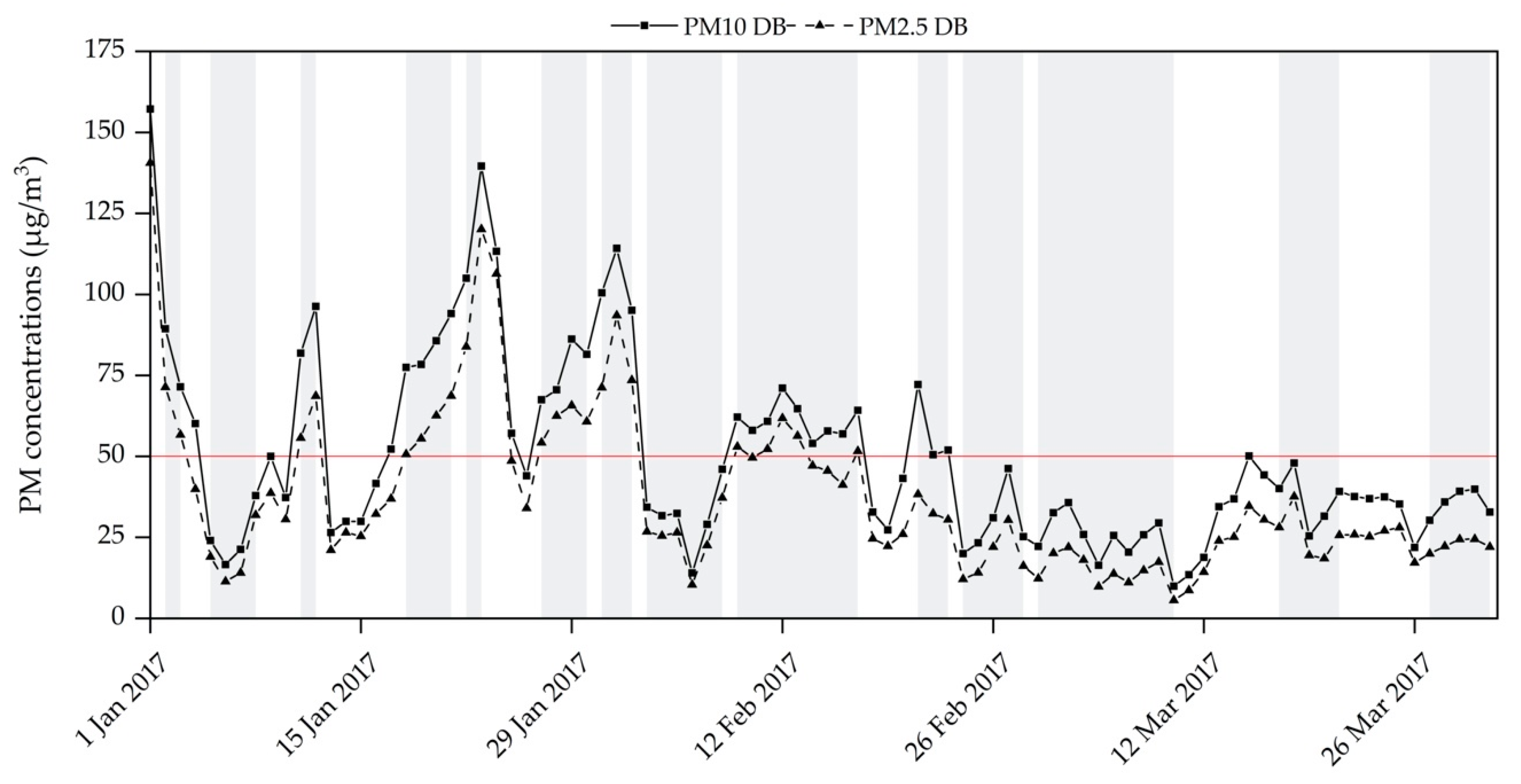
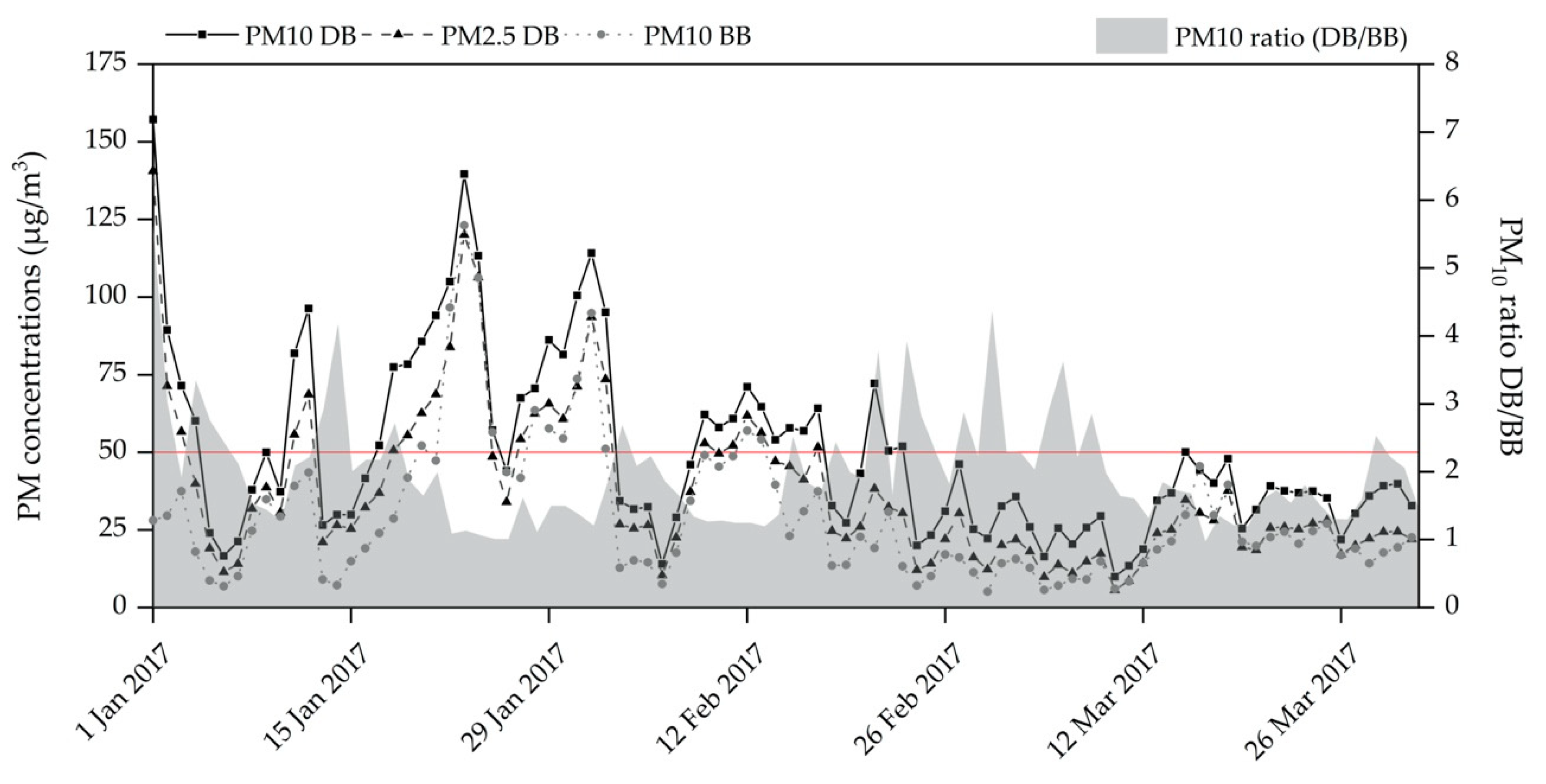
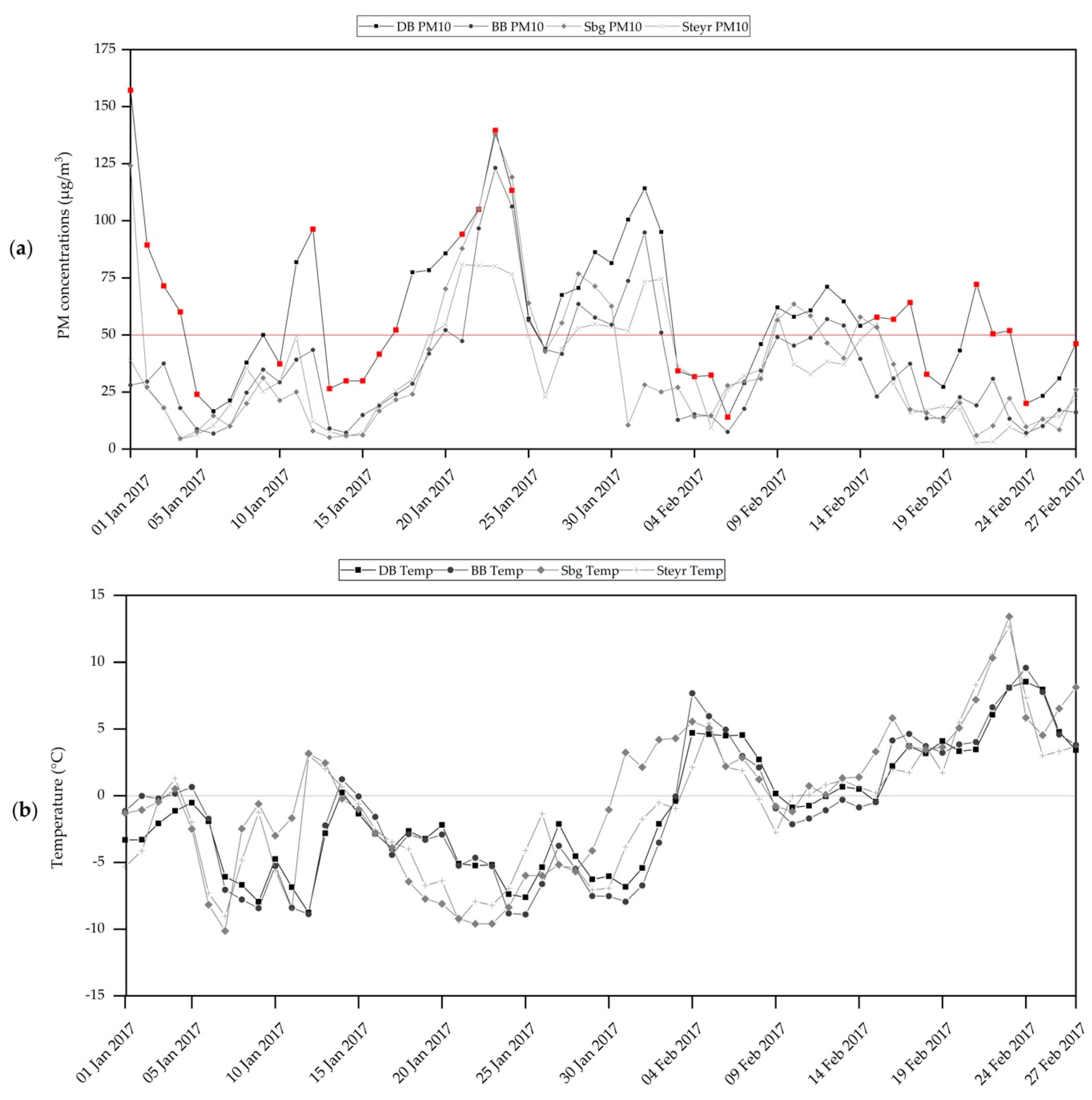
3.1. PM2.5 and PM10 Concentrations

Figure 1 shows the daily PM concentrations at the urban sampling station DB over the study period. The PM10 concentrations observed between 2 January–31 March 2017 ranged from 9.9 to 140 μg/m3. On 1 January 2017 (following fireworks on New Year’s Eve) a maximum concentration of 157 µg/m3 of PM10 mass was measured, but due to the influence of fireworks this day is excluded from further evaluations in this study. During the sampling period 34 days occurred with a PM10 concentration exceeding 50 µg/m3 and thus violating the EU short time PM10 limit value. Of these exceedance days, 21 already occurred in January 2017. Considering the whole year of 2017, 54 days violating the EU short time PM10 limit value occurred, indicating a substantial PM burden in contrast to the general decreasing trend of annually occurring days of exceedances [28]. PM2.5 concentrations at the urban sampling station DB followed the trend of PM10, with concentrations between 5.6 and 120 µg/m3, giving an average PM2.5 to PM10 ratio of 0.7.
As chemical analysis could not be performed for the whole data set, selected filters were pooled to represent characteristic time periods. The pools were formed on the basis of PM10 concentrations, and time periods selected for chemical analysis are marked with grey shading in Figure 1. In total, 14 sampling pools were analyzed, comprising 64 (out of 89) days of the sampling period. Overall, the highest PM concentrations occurred during January and are represented by six sampling pools (comprising 19 days). February and March 2017 are represented by five and three sampling pools, covering 25 and 20 days, respectively.
Figure 2 combines the daily PM concentrations at the urban sampling site DB and the background site BB. As expected, lower PM10 concentrations, ranging between 5.1 and 123 µg/m3, were observed at the background site BB. Nevertheless, individual days with high PM10 concentrations emerge in the BB record. These periods of relatively similar PM concentrations at DB and BB have been considered as indicative for pollution episodes affecting an overall wider area.
The differences in PM concentrations at DB and BB are evaluated via DB/BB PM10 ratios (Figure 2). During the whole sampling period DB/BB PM10 ratios ranged between 1.0 and 4.3, and between 1.0 and 3.9 when only days with PM10 concentrations above 50 µg/m3 are considered. Elevated PM concentrations are represented by the filter pools of the time periods of 2 January–3 January 2017, 11 January–12 January 2017, 22 January–23 January 2017, 31 January–2 February 2017, 9 February–17 February 2017, and 21 February–23 February 2017. Based on the DB/BB PM10 ratios, which indicate differences or conformity between the PM concentrations determined within the city and the background site, we postulate a subdivision of these six periods into two scenarios: (1) DB/BB PM10 ratios larger than 2 represent a pollution period with local character (i.e., a marked impact of urban emissions); (2) DB/BB PM10 ratios smaller or equal to 1.5 represent comparable PM concentrations on both sampling sites and thus indicate larger scale pollution. In the following we will refer to these scenarios as ‘scenario 1’ and ‘scenario 2’, respectively. Table 1 provides detailed information about the six time periods of interest (i.e., average temperature, average DB PM10 and DB PM2.5 concentrations, and DB/BB PM10 ratios). PM ratios smaller than 1.5 or larger than 2.0 were found in March as well but were not evaluated in detail because of PM10 concentrations below the daily limit value.
Concentrations of both PM10 and PM2.5 at DB were higher during periods with temperatures below 0 °C, independent of the scenario. The PM2.5/PM10 ratio at DB was found to be lower during time periods characterized as scenario 1 (average PM2.5/PM10 ratio 0.68) than for scenario 2 (average PM2.5/PM10 ratio 0.82).

3.2. Chemical Composition

The mean values, standard deviations, and ranges for quantified PM2.5 constituents are summarized in Table 2. A list showing ambient concentrations for all analytes and sample pools is given in Table S2.

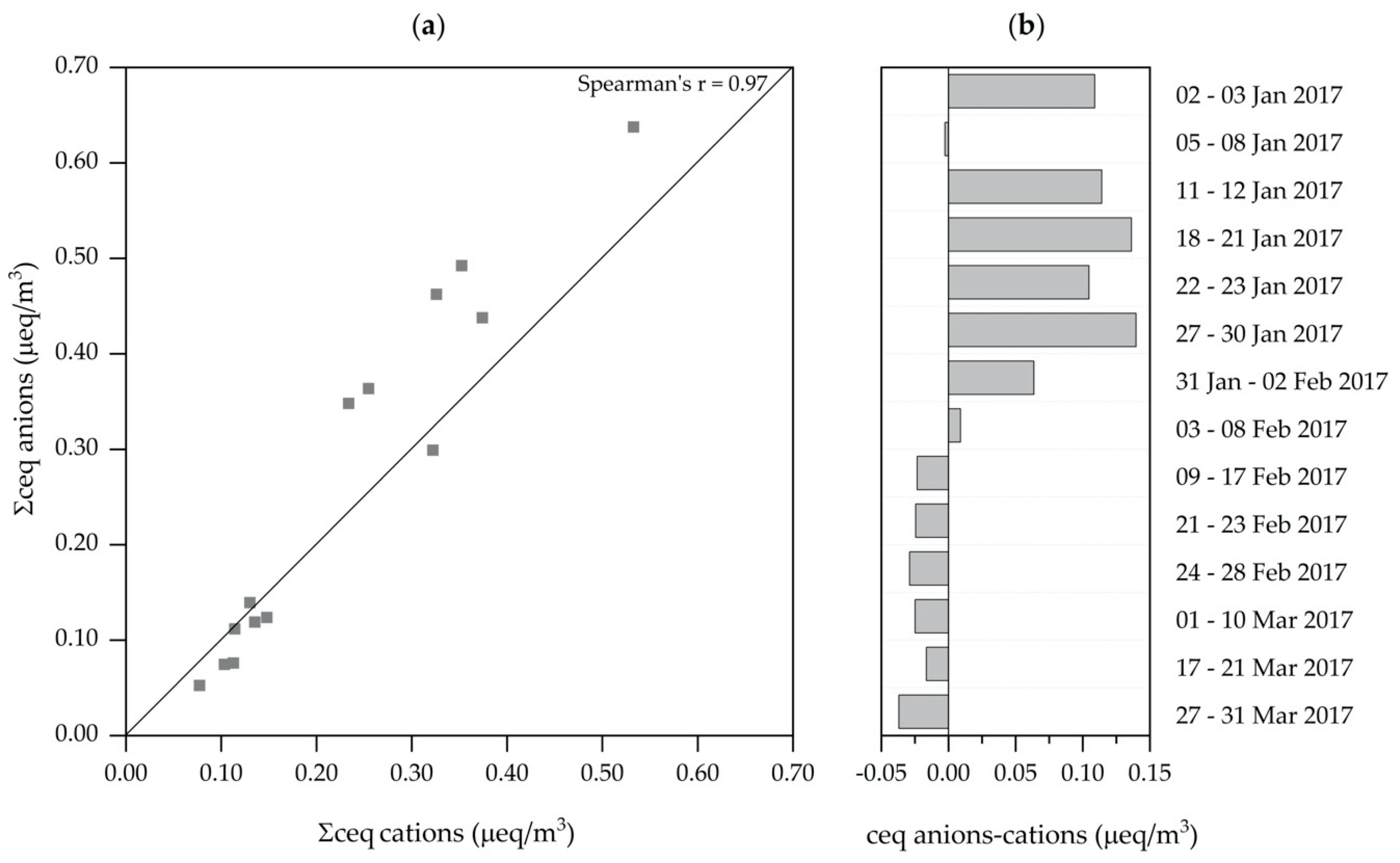
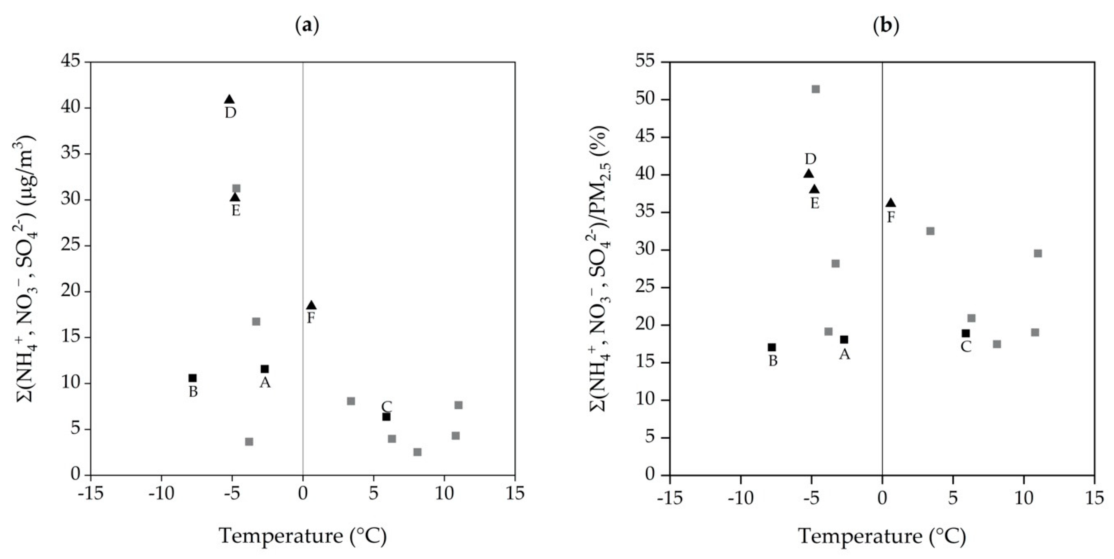
3.2.1. Ionic Composition

Mean concentrations of ionic species, as well as standard deviations, medians, and ranges are summarized in Table 2. Quantified anions contributed an average of 27% to the total PM2.5 mass, with maximum contributions of 45% (27 January–30 January 2017) and minimum contributions of 18% (27 March–31 March 2017). Total cation mass contributions were 12% on average and ranged between 8% and 14% of the total PM2.5 concentration. Overall equivalent concentrations of cations and anions are well balanced with an average value of 0.97 (Figure 3a), but show a distinct temporal evolution (Figure 3b). At the beginning of the sampling period a cation deficit emerges, which vanishes in early February with changing ambient conditions. This shift is primarily caused by decreasing concentrations of anions and ammonium, while the concentrations of the other cations remain rather constant over time, or in the case of magnesium and calcium, even show an increasing tendency. We link these changes to an increasing influence of resuspension of mineral dust, which will occur predominantly in the coarse fraction, but slightly affects PM2.5 as well [4]. Regarding the anion deficit we assume the occurrence of different anions like carbonate, but also organic acids and phosphate, which were not quantified in this study.
Elevated chloride concentrations were only found during January, concurrent with above average sodium concentrations. During January the molar ratio of chloride to sodium showed excess chloride with an average molar ratio of 1.4, while the opposite became true in February and March, where average molar ratios of 0.52 and 0.15, respectively, were observed. While the concurrent increase of sodium and chloride might indicate the use of de-icing salt applied to the urban environment, the influence of combustion sources can also contribute to the excess chloride [29,30].
Nitrate was identified as the dominant anion over the whole sampling period, with concentrations ranging between 1.6 and 20.0 µg/m3, while concentrations of sulfate ranged between 0.73 and 12.9 µg/m3 and concentrations of ammonium, the most abundant cation, ranged between 0.12 and 8.0 µg/m3. Nitrate concentrations emerge as highly correlated with sulfate (r = 0.93) and ammonium (r = 0.97), indicating the formation of (NH4)2SO4 and semi-volatile NH4NO3 [31]. Neutralization ratios based on equivalent concentrations of ammonium and sulfate showed excess ammonium for all but two sample pools with rather low PM mass in March (1 March–10 March 2017; 27 March–31 March 2017). If nitrate is included, the neutralization ratios (NH4+/∑(SO42− + NO3)) show a maximum value of 0.83, indicating that a fraction of the nitrate present is associated with other ions such as potassium (r = 0.75). These conditions allow to estimate the concentrations of (NH4)2SO4 and NH4NO3 based on the molar concentrations of sulfate and excess ammonium (each multiplied with the respective molar mass of the salt). During time periods with average ambient temperature below 0 °C the contribution of NH4NO3 to major ions (ammonium, nitrate, and sulfate) was on average 33% (up to a maximum of 47%). Conversely, during warmer periods (average temperature above 0 °C) the contribution of NH4NO3 never exceeded 26% and appeared even as negligible during some periods. The contribution of (NH4)2SO4 to major ions showed no variation with temperature (average contribution of 37% during time periods with temperatures below 0 °C and 33% during time periods above freezing, respectively). Figure 4 shows the temperature dependency of major ions presented as mass concentrations (Figure 4a) and relative contributions to PM2.5 mass (Figure 4b). The sampling periods representing the two scenarios defined before are indicated with black squares (scenario 1) and black triangles (scenario 2). Summed ammonium, nitrate, and sulfate contributed between 17% and 51% of PM2.5. A weak tendency is found towards higher contributions during periods with lower air temperatures (Figure 4b). Independently from a temperature dependence, pronounced differences in the contribution of major ions to the overall mass of PM2.5 were observed, when classification according to the DB/BB PM10 ratios is considered. During time periods with DB/BB PM10 ratios ≤ 1.5 (scenario 2) contributions were rather high (36–40%), compared to periods with DB/BB PM10 ratios > 2 (scenario 1; 17–19%). Even during the coldest time span of the study period (11 January–12 January 2017, average T= −7.8 °C), the contribution of nitrate, sulfate, and ammonium yielded only 17%. The classifications according to the DB/BB PM10 ratio indicate a more pronounced influence of secondary inorganic ions during time periods characterized by transport of air pollutants. The differentiation according to the DB/BB PM10 ratios is also reflected by the neutralization ratios (NH4+/∑(SO42− + NO3). These are higher during periods characterized by scenario 2 (average value of 0.72) than scenario 1 (average neutralization ratio of 0.49). Likewise, the contribution of NH4NO3, calculated as above, to major ions differs. It was found to be higher during time periods of scenario 2 (30%) than during time periods of scenario 1 (16%), although the time periods representing scenario 1 were characterized by lower temperatures. Average concentrations of sodium, calcium, and chloride are slightly higher during time periods with DB/BB PM10 ratios > 2 (i.e., when urban sources dominate).
Overall ion concentrations observed during winter 2017 showed slightly lower contributions of nitrate and sulfate to PM2.5 (15% and 8%, respectively) than previously observed [12]. During time periods with elevated PM2.5 concentrations (>50 µg/m3), the average contributions of nitrate to PM2.5 mass were in a comparable range for the present and previous study (accounting to 18% in 2017 and <20% of PM2.5 mass in 2000/2001). For sulfate, lower contributions to PM2.5 (11%) were observed during time periods in 2017, while higher contributions (>20%) were reported in 2000/2001 [12]. This difference can be attributed to generally decreasing SO2 emissions [32].

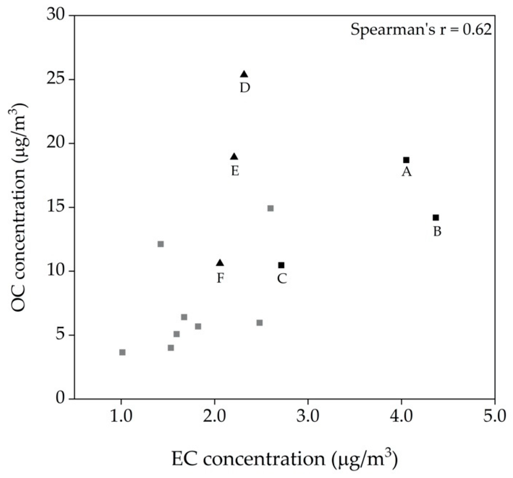
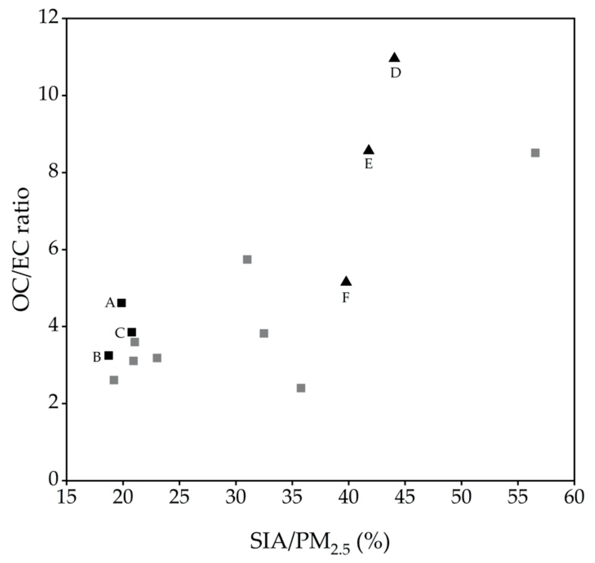
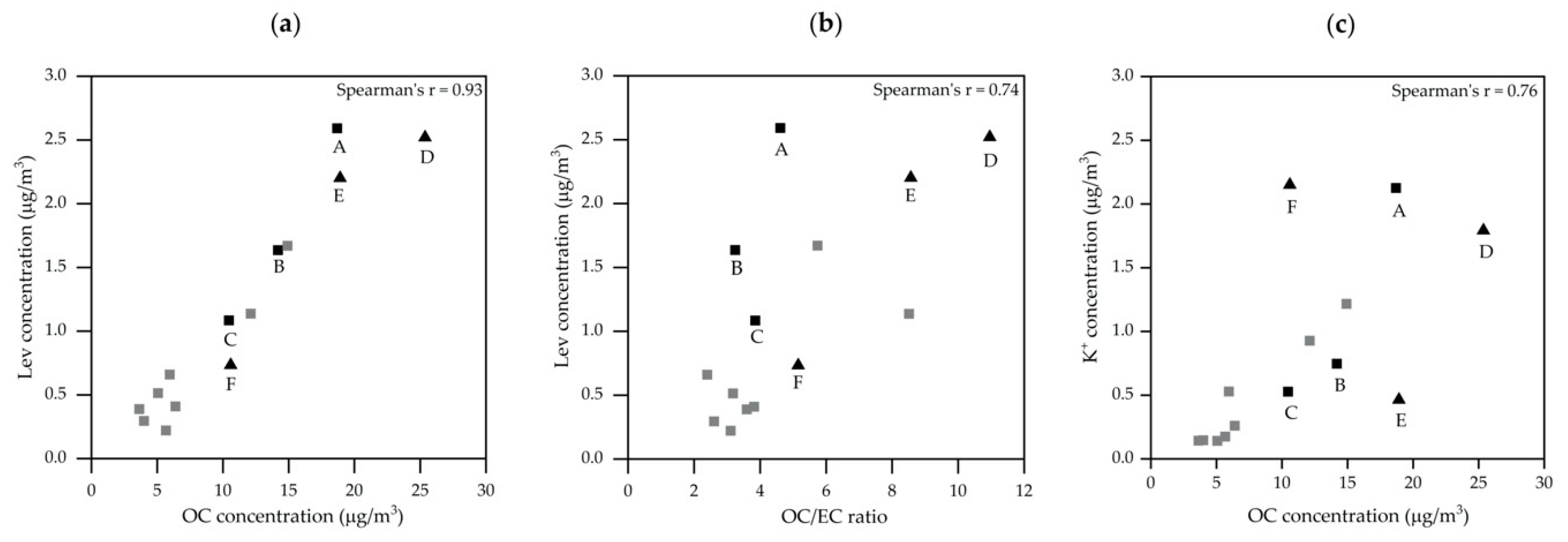
3.2.2. Carbonaceous Compounds

Average OC and EC concentrations as well as the standard deviations, median values, and ranges are summarized in Table 2. Figure 5 shows the correlation between OC and EC concentrations, as the OC/EC ratio is commonly used to distinguish between different sources of carbonaceous material [33]. Previous studies reported lower OC/EC ratios (up to 2.3) to be associated with fossil fuel burning, while OC/EC ratios associated to emissions from biomass combustion are higher and exhibit a wider range (up to 16) [29,33,34]. The OC/EC ratios found in this study ranged from 2.4 to 11. The classification according to DB/BB PM10 ratios characterizes differences in chemical composition and possible aerosol sources (Figure 5). Scenario 2 (DB/BB PM10 ratios ≤ 1.5) shows higher OC/EC ratios (5.2 to 11), characteristic for aerosols related to biomass burning, while scenario 1 (DB/BB PM10 ratios > 2) yields samples with lower OC/EC ratios (3.2 to 4.6) indicating the influence of biomass burning as well as fossil fuel combustion and thereby a plausible, stronger urban impact.
The highest OC/EC ratios (>5) occurred when ambient temperatures were rather low (until mid-February), pointing to a pronounced influence of biomass combustion. Yet, this was not accompanied with lower relative contributions of inorganic ions, as could be expected because of the increased source for carbonaceous aerosols. Figure 6 shows the correlation between OC/EC ratios and the contribution of ammonium, nitrate, and sulfate (summarized as SIA, see Section 2.4) to PM2.5. Scenario 1 shows generally lower OC/EC ratios, and also lower contributions of SIA. The opposite can be observed during time periods of scenario 2 where the more regional character of the pollution event characterized by similar PM concentrations at the urban and the background site leads to higher OC/EC ratios and an above average contribution of SIA.
The influence of biomass combustion indicated by the OC/EC ratios was further investigated using the molecular tracer levoglucosan. Emission studies linked levoglucosan (Lev), mannosan (Man), and galactosan (Gal) to biomass combustion processes [18,35], whereas the ratios of Lev/Man and Lev/Gal provide information about the combustion material [13,30]. Lev was found to be the most abundant saccharide during the sampling period with an average ambient concentration of 0.86 µg/m3 (0.22 to 2.6 µg/m3), contributing 1% to 4% of total PM2.5 mass. Atmospheric concentrations of Lev were higher during cold periods and decreased with time and increasing temperatures. Man concentrations were on average eight times lower than those of Lev, with concentrations ranging from 0.03 to 0.35 µg/m3. Average Lev/Man ratios yielded 7.9 indicative for the use of softwood and hardwood as fuel for biomass combustion [15]. Gal concentrations were mainly below the limit of detection. Figure 7a shows a high correlation between Lev and OC concentrations (r = 0.93) for the whole data set, suggesting a major fraction of OC originating from biomass burning across all samples. The correlation between Lev concentrations and OC/EC ratios (Figure 7b) shows larger scatter (r = 0.74) and some difference between samples representing different DB/BB PM10 ratios. Samples representing scenario 1 (black squares) show variable Lev concentrations but lower OC/EC ratios, while time periods of scenario 2 (black triangles) show higher OC/EC ratios despite Lev concentrations similar to scenario 1. This is mainly driven by the relative contribution of EC and the occurrence of other EC sources. During scenario 2 the average contribution of EC to PM2.5 mass is 4%, while it averages at 7% during scenario 1.
In addition, the correlation of OC with potassium (r = 0.76, Figure 7c) suggests biomass burning as a possible source of particulate matter [35,36]. Two data points associated with scenario 2 do not follow the general trend. Period F shows rather high potassium concentrations and during that time period the influence of long-range transport of desert dust appears likely [28]. No explanation can be given for the rather low potassium concentrations determined for data point E.

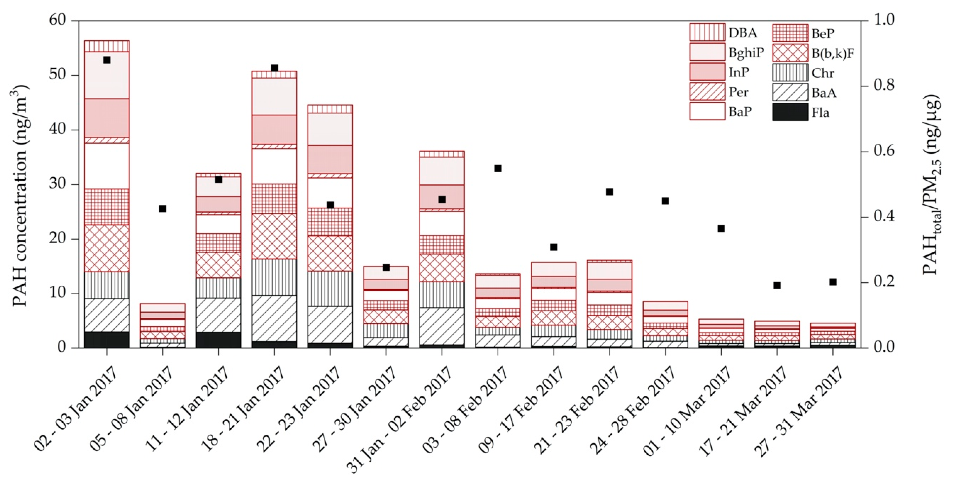
3.2.3. PM2.5 Associated PAHs

Ten PAHs including fluoranthene, benzo(a)anthracene, chrysene, benzo(b,k)fluoranthene, benzo(e)pyrene, benzo(a)pyrene, perylene, indeno(1,2,3-cd)pyrene, benzo(ghi)perylene, and dibenz(ah)anthracene were quantified for all time periods. The sum of all 10 quantified PAHs is hereinafter abbreviated as PAHtotal. Table 3 presents average PAH concentrations as well as the standard deviations, median values, and ranges for each congener associated to PM2.5 samples at Graz DB. Concentrations of benzo(a)pyrene (BaP), the primary representative of PAHs and a known carcinogen (class 1 by the International Agency for Research on Cancer (IARC) [37]), ranged between 0.51 and 8.4 ng/m3 (2.2 ng/m3). The highest concentrations of BaP was measured during 2 January–3 January 2017, a time period still showing influence of local activities at New Year’s Eve, where PAHtotal concentrations reached 102 ng/m3. PAHtotal concentrations varied from 4.6 to 56 ng/m3 (17 ng/m3) over the study period and are comparable to recent results reported for other European cities [38,39]. With proceeding time, a decreasing trend of PAHtotal concentrations was observed and highest concentrations could be observed for benzo(b,k)fluoranthene (B(b,k)F) followed by benzo(a)anthracene (BaA) and BaP.
The toxicity of PAHs is known to differ dependent on molecular weight, and many of the heaviest PAHs are categorized by IARC as already known (class 1), probable (class 2A) or possible (group 2B) human carcinogens [37]. Therefore, we grouped the quantified PAHs in middle molecular weight PAHs (MMW, containing 4-ring congeners) and high molecular weight PAHs (HMW, containing 5- and 6-ring congeners). PAH profiles are given in Figure 8. Due to their high volatility, low molecular weight PAHs containing 2- and 3-ring congeners are not included in this work. During all time periods HMW PAHs were identified as the major components with PAH concentrations ranging from 2.9 to 42 ng/m3 corresponding to 60–79% of the PAHtotal concentrations. The ratio of PAHtotal to PM2.5 ranged between 0.19 and 0.88 ng/µg and the corresponding ratios of BaP/PM2.5 varied between 0.02 and 0.13 ng/µg during the whole sampling period. With increasing time not only the observed PAH patterns changed, also the PAHtotal/PM2.5 ratios decreased (Figure 8). Generally increasing temperatures result in lower PAH emissions, due to reduced residential heating activities and higher degradation of PAHs. This is already visible towards the end of the study period, which agrees with previously reported differences between summer and winter [38,39]. A clear difference in PAHtotal/PM2.5 ratio was observed when a filter pool belonging to scenario 1 was analyzed. During that time period (21 February–23 February 2017) PAH concentrations within the city were found to be much higher than at the background site, leading to an increase in PAH/PM2.5 ratio.
Generally lower PAHtotal/PM2.5 ratios were found during time periods of scenario 2 (0.36 ng/µg) (i.e., time periods with DB/BB PM10 ratios ≤ 1.5). Time periods of scenario 1 (DB/BB PM10 ratios > 2) showed a more pronounced urban influence and thus higher PAHtotal/PM2.5 ratios (0.60 ng/µg). The highest PAH/PM2.5 ratios were found for BaP, benzo(ghi)perylene (BghiP), and B(b,k)F during time periods of scenario 1 with average ratios of 0.08 (BaP/PM2.5), 0.09 (BghiP/PM2.5) and 0.09 ng/µg (B(b,k,)F/PM2.5). Time periods of scenario 2 showed lower ratios of 0.05 ng/µg for both BaP/PM2.5 and BghiP/PM2.5 ratios and 0.06 ng/µg for B(b,k)F/PM2.5.

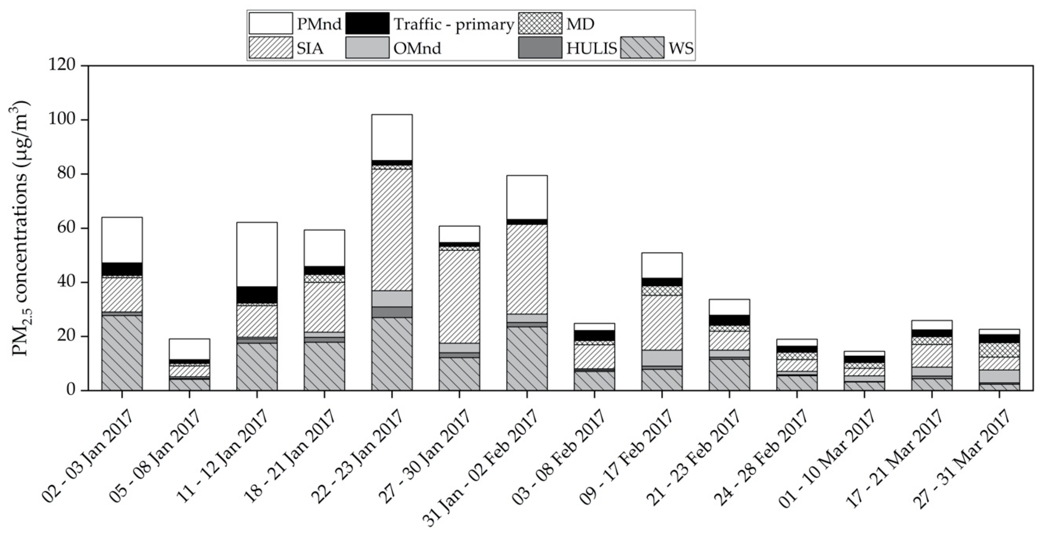
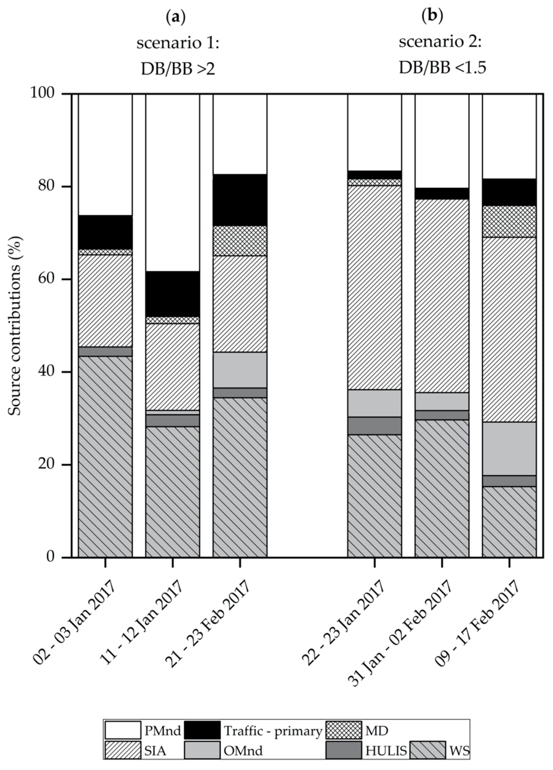
3.3. Source Apportionment with a Macro-Tracer Approach

The concentrations of the PM source groups defined in Section 2.4 are shown in Figure 9. For all sample pools WS and SIA emerge as the dominant sources, although with alternating dominance. WS contributions to PM2.5 mass ranged between 10% and 43% (2.4–27.7 µg/m3) and contributions from SIA ranged between 19% and 57% (2.8–44.9 µg/m3). Contributions of ‘traffic primary’ ranged between 1.6% and 16% (1.4–6.0 µg/m3). Contributions of HULIS and MD showed rather low average contributions to PM2.5 mass of 2.3% (1.0 µg/m3) and 4.1% (2.2 µg/m3), respectively. Uncertainties in conversion factors lead to under- and over-estimations of PM sources in certain cases. However, during the study period the carbonaceous fraction was slightly overestimated (1.8 µg/m3) only between 2 January–3 January 2017 via this macro-tracer approach.
As the discussions of the chemical composition revealed marked differences between the two scenarios, source apportionment via the macro-tracer approach is shown in more detail for these samples (Figure 10). Time periods of scenario 1 (DB/BB PM10 ratios > 2; Figure 10a) showed higher average contributions of ‘traffic primary’, contributing 7–11% to PM2.5 mass (average value of 10%), while contributions of SIA ranged from 19–21% (average value of 20%). Contributions of WS ranged between 28% and 43% (average value of 35%). Furthermore, the mass of not identified PM was found quite high. During time periods of scenario 2 (DB/BB PM10 ratios ≤ 1.5; Figure 10b), SIA increased and ranged from 40–44%, even though these days were not the coldest during the study period. During this scenario the contribution of ‘traffic primary’ decreased to an average value of 4%. Contributions of WS ranged from 15–30% (average value of 20%), and thus are lower than during samples of scenario 1. The time period of 9 February–17 February 2017 shows elevated contributions of MD and also OMnd, which can be linked to an input of desert dust identified during this time period [28]. Generally speaking, MD did not show pronounced variations during either scenario considered (4% during scenario 1 and 5% during scenario 2). The same was found for HULIS, with average contributions of 2% and 3%, respectively. Contributions of OMnd were found to be higher during time periods of scenario 2 (9%) than during scenario 1 (2%).
Thus, the simple classification based on the difference in DB/BB PM10 ratios (local vs. regional) is reflected by chemical characterization and findings of source apportionment.

Supporting Information from Meteorological Analyses

The chemical analyses described above detail the PM source apportionment to individual subgroups/components of interest. To supplement the findings of the chemical analyses regarding contributions from local and regional emissions to PM burdens meteorological data is analyzed. Today it is well understood that ambient meteorological conditions strongly modulate PM burdens and determine particulate accumulation and decay [40,41,42,43]. High PM burdens coincide normally with one or multiple of the following meteorological phenomena: stagnant weather conditions, calm winds and limited ventilation, cold ambient temperatures leading to a shallow boundary layer, and temperature inversions inhibiting vertical mixing.
To characterize the meteorological conditions on a regional basis we used the WLKC733 weather classification [44], which provides information on dominant wind direction, cyclonicity at 925 hPa and 500 hPa, and dominance of wet or dry conditions. To characterize local meteorological conditions, we considered measurements of ambient air temperature and wind direction and wind speed. Of these covariates, temperature is most important as it is relatively variable over the study period. Wind speeds are generally modest in Graz during winter times. Over the study period daily mean wind speed was found for most days to be below 1.5 m/s (and daily maxima below 3 m/s). As the city of Graz is prone to temperature inversions, due to its valley location, we diagnosed the presence of a local temperature inversion by determining the air temperature gradient from measurements at the sites DB and Kalkleiten (at ~12 km distance located on a hill encompassing the basin).
From a meteorological perspective stagnant conditions were dominating during January and February 2017. Furthermore, extended periods with cold temperatures (<0 °C) occurred, particularly during January, favoring PM accumulation within the shallow boundary layer (Figure 11b). Chemical source apportionment indicates predominantly widespread regional pollution events besides the sample pools spanning 2 January–3 January 2017, 11 January–12 January 2017, and 21 February–23 February 2017. The regional uniform evolution of ambient air temperatures indicates a relatively homogeneous boundary layer as its depth is determined by ambient temperatures. This is mirrored in the parallel evolution of PM burdens across Styrian air quality monitoring sites (Figure 11a). The highest PM burden is found for the PM pool sampled during the time period of 22 January–23 January 2017. Meteorological data indicate a particularly shallow boundary layer in combination with stagnation. In addition, meteorological data for the city of Graz indicates the presence of a temperature inversion (red highlighted symbols in Figure 11a). Contrasting PM data for DB with those of other Styrian and Austrian sites indicate however, that this local inversion is not the dominant driver of PM pollution. In fact, widespread increases in PM abundance have been reported on a larger scale due to enhanced European pollution backgrounds [6]. In contrast, the PM pools sampled during 2 January–3 January 2017, 11 January–12 January 2017, and 21 February–23 February 2017 carry the signature of an enhanced contribution of local urban emissions to the Graz PM burden. For both periods a local temperature inversion is diagnosed for Graz. Contrasting PM burdens for DB with data from the site BB and Hartberg indicate that this temperature inversion has been a localized phenomenon trapping urban emissions within the boundary layer. For the data pool sampled during 9 February–17 February 2017 stagnant conditions were diagnosed. The regionally homogeneous cold temperatures indicate a shallow boundary layer and combined consideration of urban, rural, and background monitoring sites indicates a regionally enhanced PM background.

4. Summary and Conclusions

The study presents results of the chemical characterization and source apportionment of atmospheric PM2.5 at an urban monitoring station in Graz, Austria during January to March 2017. The chosen sampling station is a known hotspot for elevated PM10 concentrations in Austria. Given the limited number of samples, source apportionment was performed via an exploratory method using specific marker compounds and conversion factors optimized for the region of interest. Building on this study, future work is suggested, which should include a detailed analysis of longer time periods to allow the application of more comprehensive receptor models such as positive matrix factorization.
Based on the comparison of the PM ratios between an urban (DB) and background (BB) site (DB/BB PM10 ratios), two scenarios were identified: (1) time periods with DB/BB PM10 ratios > 2, indicating dominant urban impact; (2) time periods with DB/BB PM10 ratios ≤ 1.5, which characterize pollution episodes observed across a wider area. Pronounced differences in the chemical characterization of the respective samples and in source apportionment show the feasibility of this simple ‘dual-site’ approach.
Time periods with DB/BB PM10 ratios > 2: Several PM2.5 associated components (e.g., EC, PAHs) were found at elevated fractions during these time periods indicating a dominant influence of urban sources. Higher EC contributions as well as ratios of individual PAHs/PM2.5 related to traffic emissions and combustion pointed towards a pronounced local influence. According to source apportionment the influence of ‘traffic primary’ is markedly higher, but also WS is a dominant source. This is also indicated by OC/K+ correlations and levoglucosan concentrations.
Time periods with DB/BB PM10 ratios ≤ 1.5: Time periods have been identified as regional pollution episodes, indicated, for example, by a strong increase of the contribution of SIA. The largest ammonium and nitrate inputs were observed within these time periods, with elevated levels not only found during cold spells. Samples representing scenario 2 also showed differences in OC/K+ correlation and the macro-tracer derived source apportionment showed a clear dominance of SIA. WS emerged as the second most important aerosol source.
The comparison of the results of the chemical analyses with supporting meteorological information showed the presence of inversions during time periods with DB/BB PM10 ratios > 2. These local inversions favored the accumulation of locally produced PM. On the other hand, the comparison of meteorological data across a wider area indicated that during other time periods high PM background concentrations occurred. During these episodes, local inversion, even if present, does not appear as the primary driver of elevated PM concentrations.

Supplementary Materials

The following are available online at https://0-www-mdpi-com.brum.beds.ac.uk/2076-3417/10/12/4222/s1, Table S1: List of conversion factors to calculate the source contribution; Table S2: Summary of ambient concentrations of quantified analytes related to PM2.5 at Graz DB.

Author Contributions

Conceptualization of the study was done by B.K. and A.K.-G.; chemical analyses were done by B.K., M.K., T.S., C.H., and A.L.; meteorological data was interpreted and prepared by C.S. and H.R.; writing and original draft preparation was done by B.K.; writing—review and editing was done by A.K.-G. and H.R. All authors have read and agree to the published version of the manuscript.

Funding

This research was partly funded by the provincial government of Styria. Open Access Funding by TU Wien.

Acknowledgments

The authors wish to acknowledge the provincial government of Styria for providing the filter material and air quality monitoring data and for partially funding the analysis. H. R. and C. S. acknowledge financial support by the provincial state government of Styria and the Environment Agency of the city of Graz. The authors acknowledge the Austrian Environment Agency and provincial governments of Upper Austria and Salzburg for providing air quality and meteorological data as well as ZAMG for providing WLKC733. The APC was funded by TU Wien University Library through its Open Access Funding Program.

Conflicts of Interest

The authors declare no conflict of interest.

References

  1. WHO. Health Effects of Particulate Matter-Policy Implications for Countries in Eastern Europe, Caucasus and Central Asia; WHO: Geneva, Switzerland, 2013. [Google Scholar]
  2. WHO. Air Quality Guidelines for Particulate Matter, Ozone, Nitrogen Dioxide and Sulfur Dioxide, Global Update 2005; WHO: Geneva, Switzerland, 2005. [Google Scholar]
  3. WHO. Sustainable Development Goals (SDGs). Available online: https://www.who.int/sdg/en/ (accessed on 21 April 2020).
  4. Puxbaum, H.; Gomiscek, B.; Kalina, M.; Bauer, H.; Salam, A.; Stopper, S.; Preining, O.; Hauck, H. A dual site study of PM 2.5 and PM 10 aerosol chemistry in the larger region of Vienna, Austria. Atmos. Environ. 2004, 38, 3949–3958. [Google Scholar] [CrossRef]
  5. Lenschow, P.; Abraham, H.J.; Kutzner, K.; Lutz, M.; Preuß, J.D.; Reichenbächer, W. Some ideas about the sources of PM10. Atmos. Environ. 2001, 35, S23–S33. [Google Scholar] [CrossRef]
  6. EEA. Air Quality in Europe-2019 Report; EEA: Copenhagen, Denmark, 2019. [Google Scholar] [CrossRef]
  7. Almbauer, R.A.; Oettl, D.; Bacher, M.; Sturm, P.J. Simulation of the air quality during a field study for the city of Graz. Atmos. Environ. 2000, 34, 4581–4594. [Google Scholar] [CrossRef]
  8. Iinuma, Y.; Engling, G.; Puxbaum, H.; Herrmann, H. A highly resolved anion-exchange chromatographic method for determination of saccharidic tracers for biomass combustion and primary bio-particles in atmospheric aerosol. Atmos. Environ. 2009, 43, 1367–1371. [Google Scholar] [CrossRef]
  9. Limbeck, A.; Handler, M.; Neuberger, B.; Klatzer, B.; Puxbaum, H. Carbon-specific analysis of humic- like substances in atmospheric aerosol and precipitation samples. Anal. Chem. 2005, 77, 7288. [Google Scholar] [CrossRef]
  10. Limbeck, A.; Handler, M.; Puls, C.; Zbiral, J.; Bauer, H.; Puxbaum, H. Impact of mineral components and selected trace metals on ambient PM10 concentrations. Atmos. Environ. 2009, 43, 530–538. [Google Scholar] [CrossRef]
  11. Belis, C.A.; Karagulian, F.; Larsen, B.R.; Hopke, P.K. Critical review and meta- analysis of ambient particulate matter source apportionment using receptor models in Europe. Atmos. Environ. 2013, 69, 94–108. [Google Scholar] [CrossRef]
  12. Putaud, J.P.; Van Dingenen, R.; Alastuey, A.; Bauer, H.; Birmili, W.; Cyrys, J.; Flentje, H.; Fuzzi, S.; Gehrig, R.; Hansson, H.C.; et al. A European aerosol phenomenology–3: Physical and chemical characteristics of particulate matter from 60 rural, urban, and kerbside sites across Europe. Atmos. Environ. 2010, 44, 1308–1320. [Google Scholar] [CrossRef]
  13. Caseiro, A.; Bauer, H.; Schmidl, C.; Pio, C.A.; Puxbaum, H. Wood burning impact on PM 10 in three Austrian regions. Atmos. Environ. 2009, 43, 2186–2195. [Google Scholar] [CrossRef]
  14. Kistler, M.; Kasper-Giebl, A.; Cetintas, C.; Ramirez Sanata-Cruz, C.; Schreiner, E.; Sampaio Cordeiro-Wagner, L.; Szidat, S.; Zhang, Y.; Bauer, H. PMInter Project, Analysis of Filters and 14C Measurments in Fine Particulate Matter; CTA-EAC-12/13-7; Institute of Chemical Technologies and Analytics, TU Wien: Vienna, Austria, 2013. [Google Scholar]
  15. Schmidl, C.; Marr, I.L.; Caseiro, A.; Kotianová, P.; Berner, A.; Bauer, H.; Kasper-Giebl, A.; Puxbaum, H. Chemical characterisation of fine particle emissions from wood stove combustion of common woods growing in mid-European Alpine regions. Atmos. Environ. 2008, 42, 126–141. [Google Scholar] [CrossRef]
  16. Bauer, H.; Marr, I.; Kasper-Giebl, A.; Limbeck, A.; Caseiro, A.; Handler, M.; Jankowski, N.; Klatzer, B.; Kotianova, P.; Pouresmaeil, P.; et al. “Aquella” Steiermark Endbericht-Bestimmung von Immissionsbeiträgen in Feinstaubproben; Austrian Academy of Sciences Press: Graz, Austria, 2007. [Google Scholar]
  17. Viana, M.; Kuhlbusch, T.A.J.; Querol, X.; Alastuey, A.; Harrison, R.M.; Hopke, P.K.; Winiwarter, W.; Vallius, M.; Szidat, S.; Prévôt, A.S.H.; et al. Source apportionment of particulate matter in Europe: A review of methods and results. J. Aerosol Sci. 2008, 39, 827–849. [Google Scholar] [CrossRef]
  18. Simoneit, B.R.T.; Schauer, J.J.; Nolte, C.G.; Oros, D.R.; Elias, V.O.; Fraser, M.P.; Rogge, W.F.; Cass, G.R. Levoglucosan, a tracer for cellulose in biomass burning and atmospheric particles. Atmos. Environ. 1999, 33, 173–182. [Google Scholar] [CrossRef]
  19. Vicente, E.D.; Alves, C.A. An overview of particulate emissions from residential biomass combustion. Atmos. Res. 2018, 199, 159–185. [Google Scholar] [CrossRef]
  20. Handler, M.; Puls, C.; Zbiral, J.; Marr, I.; Puxbaum, H.; Limbeck, A. Size and composition of particulate emissions from motor vehicles in the Kaisermühlen-Tunnel, Vienna. Atmos. Environ. 2008, 42, 2173–2186. [Google Scholar] [CrossRef]
  21. Limbeck, A.; Handler, M.; Puls, C.; Puxbaum, H. Bestimmung der Partikel-Emissionen (PM10) von Kraftfahrzeugen; Bundesministerium für Verkehr, Innovation und Technologie, Bundesstraßenverwaltung: Vienna, Austria, 2006. [Google Scholar]
  22. Anderl, M.; Gangl, M.; Haider, S.; Lampert, C.; Perl, D.; Poupa, S.; Purzner, M.; Schieder, W.; Titz, M.; Stranner, G.; et al. Emissionstrends 1990–2017, Ein Überblick über die Verursacher von Luftschadstoffen in Österreich (Datenstand 2019); REP-0698; EMAS: Vienna, Austria, 2019. [Google Scholar]
  23. Anderl, M.; Gangl, M.; Haider, S.; Köther, T.; Lampert, C.; Pazdernik, K.; Perl, D.; Pinterits, M.; Poupa, S.; Purzner, M.; et al. Austria’s Informative Inventory Report (IRR) 2020; REP-0723; EMAS: Vienna, Austria, 2020. [Google Scholar]
  24. Wedepohl, K.H. The composition of the continental crust. Geochim. Cosmochim. Acta 1995, 59, 1217–1232. [Google Scholar] [CrossRef]
  25. Kistler, M. Particulate Matter and Odor Emission Factors from Small Scale Biomass Combustion Units. Ph.D. Thesis, University of Technology, Vienna, Austria, 2012. [Google Scholar]
  26. Puxbaum, H.; Caseiro, A.; Sanchez-Ochoa, A.; Kasper-Giebl, A.; Claeys, M.; Gelencser, A.; Legrand, M.; Preunkert, S.; Pio, C. Levoglucosan levels at background sites in Europe for assessing the impact of biomass combustion on the European aerosol background. J. Geophys. Res.-Atmos. 2007, 112. [Google Scholar] [CrossRef] [Green Version]
  27. El-Zanan, H.S.; Lowenthal, D.H.; Zielinska, B.; Chow, J.C.; Kumar, N. Determination of the organic aerosol mass to organic carbon ratio in IMPROVE samples. Chemosphere 2005, 60, 485–496. [Google Scholar] [CrossRef]
  28. Amt der Steiermärkischen Landesregierung, A.E. Luftgütemessungen in der Steiermark-Jahresbericht 2017; Bericht Nr. Lu-07-2018; EMAS: Vienna, Austria, 2018. [Google Scholar]
  29. Kaskaoutis, D.G.; Grivas, G.; Theodosi, C.; Tsagkaraki, M.; Paraskevopoulou, D.; Stavroulas, I.; Liakakou, E.; Gkikas, A.; Hatzianastassiou, N.; Wu, C.; et al. Carbonaceous Aerosols in Contrasting Atmospheric Environments in Greek Cities: Evaluation of the EC-tracer Methods for Secondary Organic Carbon Estimation. Atmosphere 2020, 11, 161. [Google Scholar] [CrossRef] [Green Version]
  30. Fourtziou, L.; Liakakou, E.; Stavroulas, I.; Theodosi, C.; Zarmpas, P.; Psiloglou, B.; Sciare, J.; Maggos, T.; Bairachtari, K.; Bougiatioti, A.; et al. Multi-tracer approach to characterize domestic wood burning in Athens (Greece) during wintertime. Atmos. Environ. 2017, 148, 89–101. [Google Scholar] [CrossRef]
  31. Stelson, A.W.; Seinfeld, J.H. Relative humidity and temperature dependence of the ammonium nitrate dissociation constant. Atmos. Environ. 1982, 16, 983–997. [Google Scholar] [CrossRef]
  32. Greilinger, M.; Schöner, W.; Winiwarter, W.; Kasper-Giebl, A. Temporal changes of inorganic ion deposition in the seasonal snow cover for the Austrian Alps (1983–2014). Atmos. Environ. 2016, 132, 141–152. [Google Scholar] [CrossRef] [Green Version]
  33. Pio, C.; Cerqueira, M.; Harrison, R.M.; Nunes, T.; Mirante, F.; Alves, C.; Oliveira, C.; Sanchez de La Campa, A.; Artíñano, B.; Matos, M. OC/EC ratio observations in Europe: Re-thinking the approach for apportionment between primary and secondary organic carbon. Atmos. Environ. 2011, 45, 6121–6132. [Google Scholar] [CrossRef]
  34. Tolis, E.I.; Saraga, D.E.; Lytra, M.K.; Papathanasiou, A.C.; Bougaidis, P.N.; Prekas-Patronakis, O.E.; Ioannidis, I.I.; Bartzis, J.G. Concentration and chemical composition of PM2.5 for a one-year period at Thessaloniki, Greece: A comparison between city and port area. Atmos. Environ. 2015, 113, 197–207. [Google Scholar] [CrossRef]
  35. Jordan, T.; Seen, A.; Jacobsen, G. Levoglucosan as an atmospheric tracer for woodsmoke. Atmos. Environ. 2006, 40, 5316–5321. [Google Scholar] [CrossRef]
  36. Pio, C.A.; Legrand, M.; Alves, C.A.; Oliveira, T.; Afonso, J.; Caseiro, A.; Puxbaum, H.; Sanchez-Ochoa, A.; Gelencsér, A. Chemical composition of atmospheric aerosols during the 2003 summer intense forest fire period. Atmos. Environ. 2008, 42, 7530–7543. [Google Scholar] [CrossRef]
  37. IARC. Some Non-heterocyclic Polycyclic Aromatic Hydrocarbons and Some Related Exposures. In IARC Monographs on the Evaluation of Carcinogenic Risk to Humans; IARC: Lyon, France, 2010; Volume 92. [Google Scholar]
  38. Khan, M.; Masiol, M.; Bruno, C.; Pasqualetto, A.; Formenton, G.; Agostinelli, C.; Pavoni, B. Potential sources and meteorological factors affecting PM 2.5 -bound polycyclic aromatic hydrocarbon levels in six main cities of northeastern Italy: An assessment of the related carcinogenic and mutagenic risks. Environ. Sci. Pollut. Res. 2018, 25, 31987–32000. [Google Scholar] [CrossRef]
  39. Manoli, E.; Kouras, A.; Karagkiozidou, O.; Argyropoulos, G.; Voutsa, D.; Samara, C. Polycyclic aromatic hydrocarbons (PAHs) at traffic and urban background sites of northern Greece: Source apportionment of ambient PAH levels and PAH-induced lung cancer risk. Environ. Sci. Pollut. Res. 2016, 23, 3556–3568. [Google Scholar] [CrossRef]
  40. Ailish, M.G.; Kirsty, J.P.; Stephen, R.A.; Richard, J.P.; Massimo, V.; Edward, W.B.; Luke, C.; Ellen, L.S.; James, B.M. Impact of weather types on UK ambient particulate matter concentrations. Atmos. Environ. X 2020, 5. [Google Scholar] [CrossRef]
  41. Liakakou, E.; Stavroulas, I.; Kaskaoutis, D.G.; Grivas, G.; Paraskevopoulou, D.; Dumka, U.C.; Tsagkaraki, M.; Bougiatioti, A.; Oikonomou, K.; Sciare, J.; et al. Long-term variability, source apportionment and spectral properties of black carbon at an urban background site in Athens, Greece. Atmos. Environ. 2020, 222. [Google Scholar] [CrossRef]
  42. Barmpadimos, I.; Hueglin, C.; Keller, J.; Henne, S.; Prévôt, A.S.H. Influence of meteorology on PM 10 trends and variability in Switzerland from 1991 to 2008. Atmos. Chem. Phys. 2011, 11, 1813–1835. [Google Scholar] [CrossRef] [Green Version]
  43. De Hartog, J.J.; Hoek, G.; Mirme, A.; Tuch, T.; Kos, G.P.A.; Ten Brink, H.M.; Brunekreef, B.; Cyrys, J.; Heinrich, J.; Pitz, M.; et al. Relationship between different size classes of particulate matter and meteorology in three European cities. J. Environ. Monit. 2005, 7, 302–310. [Google Scholar] [CrossRef] [PubMed]
  44. Philipp, A.; Bartholy, J.; Beck, C.; Erpicum, M.; Esteban, P.; Fettweis, X.; Huth, R.; James, P.; Jourdain, S.; Kreienkamp, F.; et al. Cost733cat–A database of weather and circulation type classifications. Phys. Chem. Earth 2010, 35, 360–373. [Google Scholar] [CrossRef]
Figure 1. Daily average PM10 and PM2.5 concentrations observed at the urban sampling site Graz Don Bosco (DB). Grey shading marks selected time periods. For convenient reference, the red line marks the 50 µg/m3 limit value set by the European Commission.
Applsci 10 04222 g001
Figure 2. Daily average PM10 and PM2.5 concentrations observed at the urban sampling site DB, and daily average PM10 concentrations observed at the reference site Bockberg (BB). The grey shaded area presents the PM10 ratio between DB and BB. For convenient reference, the red line marks the 50 µg/m3 limit value set by the European Commission.
Applsci 10 04222 g002
Figure 3. (a) Ion balance of pooled PM2.5 samples at the monitoring station located in Graz Don Bosco (DB), 2 January–31 March 2017. (b) Temporal variations of ion balances for individual sampling pools.
Applsci 10 04222 g003
Figure 4. (a) Temperature dependence of mass concentrations and (b) relative contributions of major ions (nitrate, ammonium, sulfate) to PM2.5 samples at the urban sampling site in Graz DB, 2 January–31 March 2017. Black highlighted squares mark time periods with DB/BB PM10 ratios > 2 (A: 2 January–3 January 2017; B: 11 January–12 January 2017; C: 21 February–23 February 2017). Black highlighted triangles mark time periods with DB/BB PM10 ratios ≤ 1.5 (D: 22 January–23 January 2017; E: 31 January–2 February 2017 and F: 9 February–17 February 2017). Remaining data points are shown by grey squares.
Applsci 10 04222 g004
Figure 5. Scatterplot between organic carbon (OC) and elemental carbon (EC) concentrations in PM2.5 samples at the urban sampling site in Graz DB, 2 January–31 March 2017. Black highlighted squares mark time periods with DB/BB PM10 ratios > 2 (A: 2 January–3 January 2017; B: 11 January–12 January 2017; C: 21 February–23 February 2017). Black highlighted triangles mark time periods with DB/BB PM10 ratios ≤ 1.5 (D: 22 January–23 January 2017; E: 31 January–2 February 2017 and F: 9 February–17 February 2017). Remaining data points are shown by grey squares.
Applsci 10 04222 g005
Figure 6. Correlation between OC/EC ratio and the contribution of secondary inorganic aerosols (SIA) to PM2.5 at the urban sampling site in Graz DB, 2 January–31 March 2017. Black highlighted squares mark time periods with DB/BB PM10 ratios > 2 (A: 2 January–3 January 2017; B: 11 January–12 January 2017; C: 21 February–23 February 2017). Black highlighted triangles mark time periods with DB/BB PM10 ratios ≤ 1.5 (D: 22 January–23 January 2017; E: 31 January–2 February 2017 and F: 9 February–17 February 2017). Remaining data points are shown by grey squares.
Applsci 10 04222 g006
Figure 7. (ac). Correlation between levoglucosan (Lev), OC, and K+ concentrations in PM2.5 samples at the urban sampling site in Graz DB, 2 January–31 March 2017. Black highlighted squares mark time periods with DB/BB PM10 ratios > 2 (A: 2 January–3 January 2017; B: 11 January–12 January 2017; C: 21 February–23 February 2017). Black highlighted triangles mark time periods with DB/BB PM10 ratios ≤ 1.5 (D: 22 January–23 January 2017; E: 31 January–2 February 2017 and F: 9 February–17 February 2017). Remaining data points are shown by grey squares.
Applsci 10 04222 g007
Figure 8. PAH profiles according to their classification of molecular weights. Middle molecular weight (MMW) PAHs are shown in black and high molecular weight (HMW) PAHs in red. Black squares mark the PAHtotal/PM2.5 ratios.
Applsci 10 04222 g008
Figure 9. Average mass concentrations of PM2.5 source groups and undefined PM assigned by the macro-tracer method. Abbreviations: PMnd = PM not defined, MD = mineral dust, SIA = secondary inorganic aerosols, OMnd = organic material not defined, WS = wood smoke aerosol.
Applsci 10 04222 g009
Figure 10. Relative source contributions of six time periods grouped by their major differences in DB/BB PM10 ratios for sampling station Graz DB (PM2.5). Abbreviations: PMnd = PM not defined, MD = mineral dust, SIA = secondary inorganic aerosols, OMnd = organic material not defined, WS = wood smoke aerosol.
Applsci 10 04222 g010
Figure 11. (a) Time series of PM concentrations of different sampling sites in Austria including study sites DB and BB. Red highlighted data points mark days influenced by local inversion (red highlighted symbols) in Graz. (b) Time series of ambient air temperature (°C) of different monitoring sites in Austria collocated or in vicinity of the air quality monitoring sites given in (a). Abbreviations: Sbg = Salzburg.
Applsci 10 04222 g011
Table 1. Average temperature, average PM10 and PM2.5 concentrations (µg/m3) at site DB, and PM10 urban/background ratio for time periods representing scenario 1 and 2.
DateAverage Temperature (°C)DB PM10 Conc (µg/m3)DB PM2.5 Conc (µg/m3)DB/BB PM10 Ratio
2 January–3 January 2017−2.780.564.02.5
11 January–12 January 2017−7.889.162.22.2
22 January–23 January 2017−5.21221021.1
31 January–2 February 2017−4.810379.51.5
9 February–17 February 2017+0.661.150.91.5
21 February–23 February 2017+5.958.233.73.1
Table 2. Summary of ambient concentrations of major PM2.5 constituents (µg/m3) at the monitoring station located in Graz Don Bosco (DB), 2 January–31 March 2017.
Mean (µg/m3)Standard Deviation (µg/m3)Median (µg/m3)Range (µg/m3)
Cl1.52.70.920.17–7.7
NO36.46.05.31.6–20.0
SO42−3.53.72.70.73–12.9
Na+1.30.661.20.26–2.5
NH4+2.02.51.40.12–8.0
K+0.810.730.530.14–2.2
Mg2+0.060.020.060.04–0.09
Ca2+0.290.170.280.02–0.62
OC9.16.610.53.6–25.4
EC2.00.952.11.0–4.4
Lev0.860.840.910.22–2.6
Man0.110.110.120.03–0.35
Table 3. PM2.5 associated polycyclic aromatic hydrocarbons (PAHs) (ng/m3) at the urban sampling station Graz DB, 2 January–31 March 2017. Overview of 14 sample pools, except for DBA* where only 7 sample pools showed quantifiable concentrations.
AbbPAHMean (ng/m3)Standard Deviation (ng/m3)Median (ng/m3)Range (ng/m3)
FlaFluoranthene0.560.950.380.12–2.9
BaABenzo(a)anthracene2.42.91.70.45–8.4
ChrChrysene2.12.21.90.57–6.7
B(b,k)FBenzo(b,k)Fluoranthene2.72.72.60.81–8.6
BePBenzo(e)pyrene1.92.01.80.53–6.6
BaPBenzo(a)pyrene2.22.42.00.51–8.4
PerPerylene0.260.30.200.08–1.0
InPIndeno(1,2,3-cd)pyrene2.02.12.00.20–7.1
BghiPBenzo(ghi)perylene2.62.42.50.69–8.6
DBADibenzo(a,h)anthracene0.31 *0.6 *1.1 *0.28–2.0 *

