A Fast-Response Calorimeter with Dynamic Corrections for Transient Heat Transfer Measurements


1
State Key Laboratory of High Temperature Gas Dynamics, Institute of Mechanics, Chinese Academy of Sciences, Beijing 100190, China
2
School of Engineering Science, University of Chinese Academy of Sciences, Beijing 100049, China
*
Authors to whom correspondence should be addressed.
Appl. Sci. 2020, 10(17), 6143; https://0-doi-org.brum.beds.ac.uk/10.3390/app10176143
Submission received: 30 July 2020
/
Revised: 30 August 2020
/
Accepted: 2 September 2020
/
Published: 3 September 2020
(This article belongs to the Special Issue Diagnostic Methodology and Sensors Technologies)
Abstract
:Robust fast-response transient calorimeters with novel calorimeter elements have attracted the attention of researchers as new synthetic materials have been developed. This sensor uses diamonds as the calorimeter element, and a platinum film resistance is sputtered on the back to measure the temperature. The surface heat flux is obtained based on the calorimetric principle. The sensor has the advantages of high sensitivity and not being prone to erosion. However, non-ideal conditions, such as heat dissipation from the calorimeter element to the surroundings, can lead to measurement deviation and result in challenges for sensor miniaturization. In this study, a novel transient calorimeter (NTC) with two different sizes was developed using air or epoxy as the back-filling material. Numerical simulations were conducted to explain the complex heat exchange between the calorimeter element and its surroundings, which showed that it deviated from the assumption of an ideal calorimeter sensor. Accordingly, a dynamic correction method was proposed to compensate for the energy loss from the backside of the calorimeter element. The numerical results showed that the dynamic correction method significantly improved the measurement deviation, and the relative error was within 2.3% if the test time was smaller than 12 ms in the simulated cases. Detonation shock tunnel experiments confirmed the results of the dynamic correction method and demonstrated a practical method to obtain the dynamic correction coefficient. The accuracy and feasibility of the dynamic correction method were verified in a single detonation shock tunnel and under shock tube conditions. The NTC calorimeter exhibited good repeatability in all experiments.
1. Introduction
The accurate prediction of aerodynamic heating is important in the thermal and structural design of hypersonic flight vehicles, and its prediction remains a difficult problem in modern computational fluid dynamics. Experimental measurements still play an indispensable role in addressing this problem. Although much progress has been made in improving the accuracy of heat transfer measurements in recent decades, a difference of ±10% between the experimental and theoretical results is often observed, e.g., for a sharp cone standard model [1]; the difference might be even larger at certain local regions of more complex model shapes [2]. In addition, the measuring accuracy also depends on the test conditions and the sensor type. Thus, it remains necessary to extensively develop new heat flux sensors and investigate the factors influencing the heat transfer measurements before further progress can be made.
Due to the high cost of flight tests, most aerodynamic heating experiments are performed in ground facilities. And the development of experimental techniques has made it possible to achieve hypersonic flows ranging from 2.5 to 45 MJ/kg, which correspond to velocities from 2 to 10 km/s, respectively [3,4]. In such facilities, where the effective test time is on the order of milliseconds, the heat flux rate is derived from the transient temperature monitored at selected points on the model with fast response testing technology. Generally, the techniques can be divided into two categories; the first is based on heat flux sensors, such as resistance thermometers [5,6,7,8], thermocouples [9,10,11,12,13], and calorimeters [14,15,16,17], and the second is based on non-intrusive techniques such as temperature-sensitive paint [18,19] and thermography [20,21]. However, each technique has its own benefits and challenges. For example, non-intrusive optical measurements are a candidate for obtaining global temperature distribution measurements and have temporal/spatial advantages. However, the calibration procedures are very cumbersome, and the accuracy can be seriously affected by impurities of the flow field and vibration of the model. Overall, this technique remains technologically immature. Because of these optical drawbacks, point heat flux sensors, which are typically cylindrical in shape, are primarily used for heat transfer measurements [22]. These sensors must have a sufficiently fast response to obtain enough data and must withstand from thermal damage or rapid erosion due to fragments of the metallic and plastic diaphragms that hit the models at high speeds.
Among point heat flux sensors, thin-film resistance gauges have very short rise times and high electrical output per degree rise in temperature. However, they are limited to low-enthalpy flows and are prone to thermal damage or rapid erosion under high-enthalpy flows. The lifetime of each gauge is limited to one or two shots [23]. Thermocouples and calorimeters are relatively robust gauges. However, the junction of a thermocouple is formed either by mechanical interference or abrasion, which requires re-abrading or re-machining between shots due to damage from the flow. There are also uncertainties associated with the junction structures [24]. Moreover, the sensitivity of a thermocouple is relatively low at tens of microvolts per degree (about 61 μv/K for a type-E thermocouple at 300 K [25]). Besides, both thin films and thermocouples can suffer from interference from ionized flows due to exposed metallic elements [26], and insulating coatings to prevent this are typically fragile or affect the performance. In contrast, in a calorimeter-style gauge, the temperature sensing element can be shielded from direct contact with the erosive flows. This sensor also has the advantages of straightforward production and low cost and is suitable for fabrication or modification according to various requirements in the laboratory.
Calorimeter gauges are based on calculating the instantaneous heat transfer rate by measuring the time rate of change of the thermal energy in a metal element. The thermal energy is determined by obtaining a temperature measurement at the back surface of the element, and the rate of change of the temperature provides the heat flux of the exposed surface. Different types of calorimeter gauges, such as thin-wall calorimeters [14], slug calorimeters [27], and null-point calorimeters [28,29], have been developed by researchers to address the requirements of unique testing environments. Slug and null-point calorimeter gauges are generally developed for long test time measurements (such as a plasma wind tunnel), whereas a thin-wall calorimeter is more suitable for transient hypersonic facilities with testing durations on the order of milliseconds. Previous thin-wall calorimeters usually have copper as the calorimeter material and a thermocouple on the back of the calorimeter to measure the temperature rise. However, they have the same disadvantage—namely, low sensitivity—as coaxial thermocouples. Ledford [30] proposed a new design method that used an aluminum sheet as the calorimeter. In addition, the back was anodized for electrical insulation and plated with a platinum film. The back temperature of the aluminum sheet was measured by the platinum film to improve the output sensitivity of the calorimeter. However, this design was only reported in a few articles in 1960s, and there is no literature of relevance in the following years. The main reason was that cavities remained on the surface of the aluminum sheet after oxidation in the actual production process. The secondary coating resulted in conduction between the platinum film and the base material, and the platinum film did not provide insulation from the aluminum sheet. The thermal conductivity of the aluminum oxide after oxidation was also poor, adversely affecting the heat flux measurements.
The above improved design of the calorimeter can greatly improve the output sensitivity of the calorimeter, but it is necessary to find a new calorimeter material with high thermal conductivity and resistance. The thermal conductivity of natural diamonds is about 2200 W/m K, which is five times that of copper. Additionally, the resistivity is more than 1014 Ω·cm, which meets the requirements of high thermal conductivity and resistance. Thus, diamonds may be an ideal calorimetric material. Natural diamonds are expensive, but chemical vapor deposition (CVD) diamonds are relatively mature due to the development of synthetic materials [31]. Although the thermal conductivity of CVD diamonds does not reach the level of natural diamonds, it is still much higher than that of conventional metals, and the production cost is much lower. If CVD diamonds can be used to fabricate a calorimeter, the thermal response would be very fast because of the high thermal conductivity of CVD diamonds.
Due to the advantages of this new type of transient calorimeter, researchers investigated potential applications. Rowland [32] fabricated a diamond calorimeter heat transfer gauge with a diameter of 3.9 mm. The filling material of the bottom lining was glue, and experiments were conducted in an X2 expansion wind tunnel. Zhang [33] used CVD diamonds to create a novel heat transfer calorimeter with a diameter of 20 mm and air as the bottom lining material. The author performed validation experiments in a shock wind tunnel. Rowland and Zhang obtained promising results. However, the effective test time in the X2 expansion tube was short (in the order of microseconds), and the heat dissipation effect may not be serious. Although Zhang used air as the back-filling material to reduce the heat dissipation effect, the sensor size was large, which was not conducive to easy installation. As the sensor scale was reduced, the effects of transverse heat transfer and bottom heat dissipation due to the structure of the calorimeter could not be ignored, which would lead to the measurement deviation. Few studies have investigated these problems. Thus, it is necessary to perform more in-depth research.
In this study, a robust fast-response transient calorimeter using diamonds as the calorimeter element was developed for heat transfer measurements. The platinum film resistance is attached to the back of the diamond as the sensitive temperature measurement element, which significantly improves the signal output sensitivity. The temperature distribution within the gauge is then examined by solving the two-dimensional heat conduction equations numerically. Non-ideal effects of heat loss to the surrounding back-material are discussed. Further, the gauge is fully tested under three types of test conditions, exhibiting excellent performance in all these cases. In all, this developed gauge extends and supplements the high-enthalpy shock tunnel heat transfer measurements performed by other techniques.
2. Novel Transient Calorimeter (NTC)
2.1. Principe and Characteristic of the Novel Transient Calorimeter
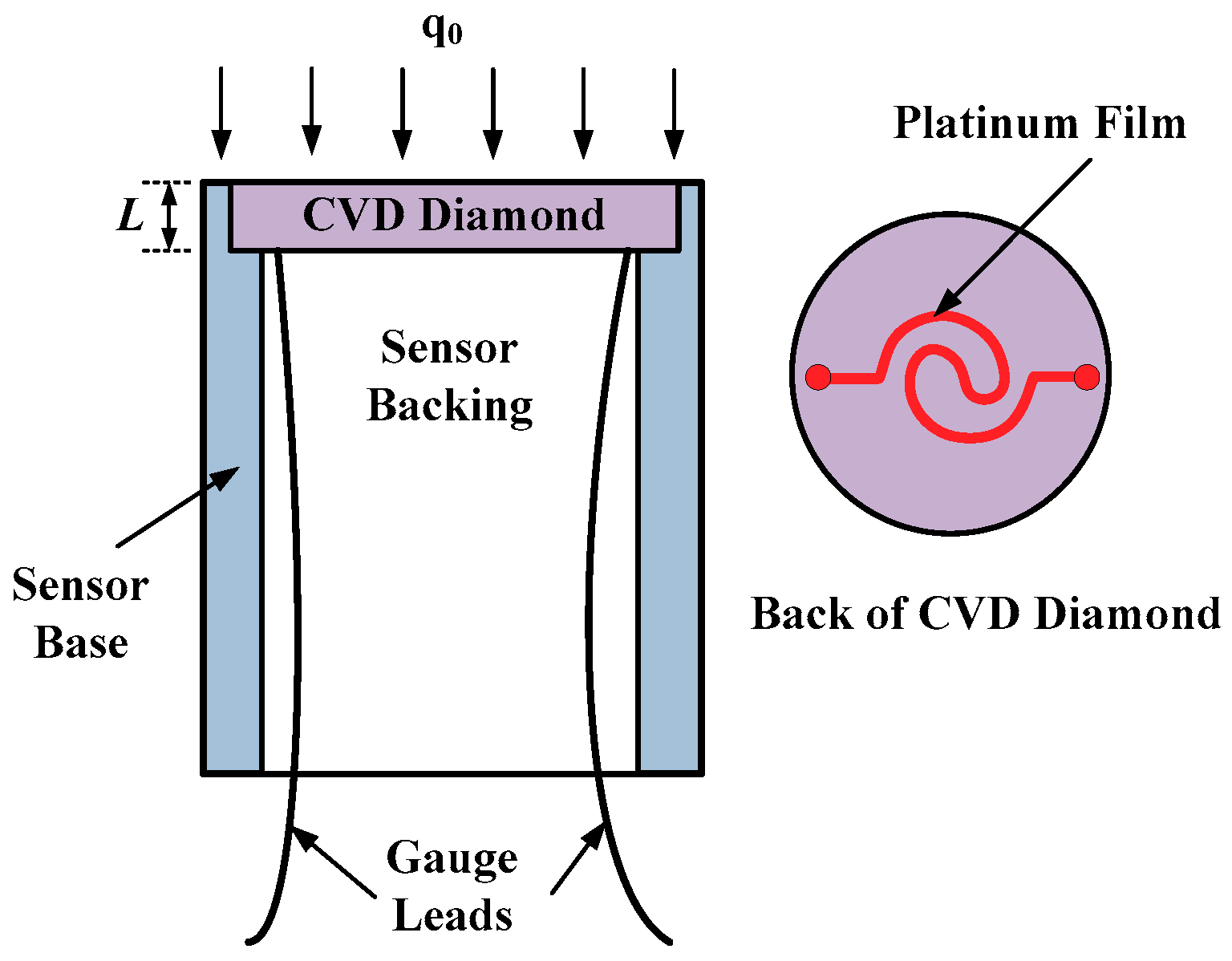
The structural diagram of the novel transient calorimeter (NTC) is shown in Figure 1. CVD diamond is selected as the calorimeter element. Firstly, the platinum film resistance is sputtered on the back of the diamond as the sensitive temperature measurement element. Subsequently, the calorimeter element is attached to the sensor base. The platinum film wire extends from the back of the calorimeter, and the bottom is filled with air or insulation material, which is usually epoxy.
The measurement principle of the transient calorimeter assumes that the back and side of the calorimeter element are adiabatic; namely, there is no heat loss from the calorimeter element. Thus, the heat introduced into the calorimeter element at certain time intervals should be equal to the heat accumulated by the calorimeter element:
where ρ and c are the density and specific heat of the calorimetric element material (CVD diamond in the present study), respectively; L is the thickness of the calorimetric element. As the density and specific heat are assumed constant, the following equation can be obtained:
where Ta is the average temperature of the calorimetric element. The heat flux can be obtained by measuring the average temperature change rate of the calorimeter. In practical measurement, the average temperature of the calorimeter is difficult to measure. Thus, the back temperature is generally measured. Instead of using thermocouples to measure the temperature in traditional calorimeters, the new transient calorimeter uses the platinum film resistance to measure the back temperature of the CVD diamond with relatively high output sensitivity.
The thermal response time of the calorimeter element is mainly related to the thermal response characteristics of the calorimeter material. The response time tR of the calorimeter was calculated as follows by Hightower [34]:
where qb is the heat flux calculated by the back temperature of the calorimeter element; q0 is the heat flux loaded on the surface, and α = k/ρc is the thermal diffusion coefficient of the calorimeter material. Table 1 shows the thermal physical parameters of a natural diamond, CVD diamond, and copper, which is the common calorimetric material. The physical parameters of the CVD diamond are determined by the Physical Property Measurement System (PPMS) of the diamond film used in this design. The physical parameters of other materials, which will be used in subsequent numerical calculations, are also listed here.
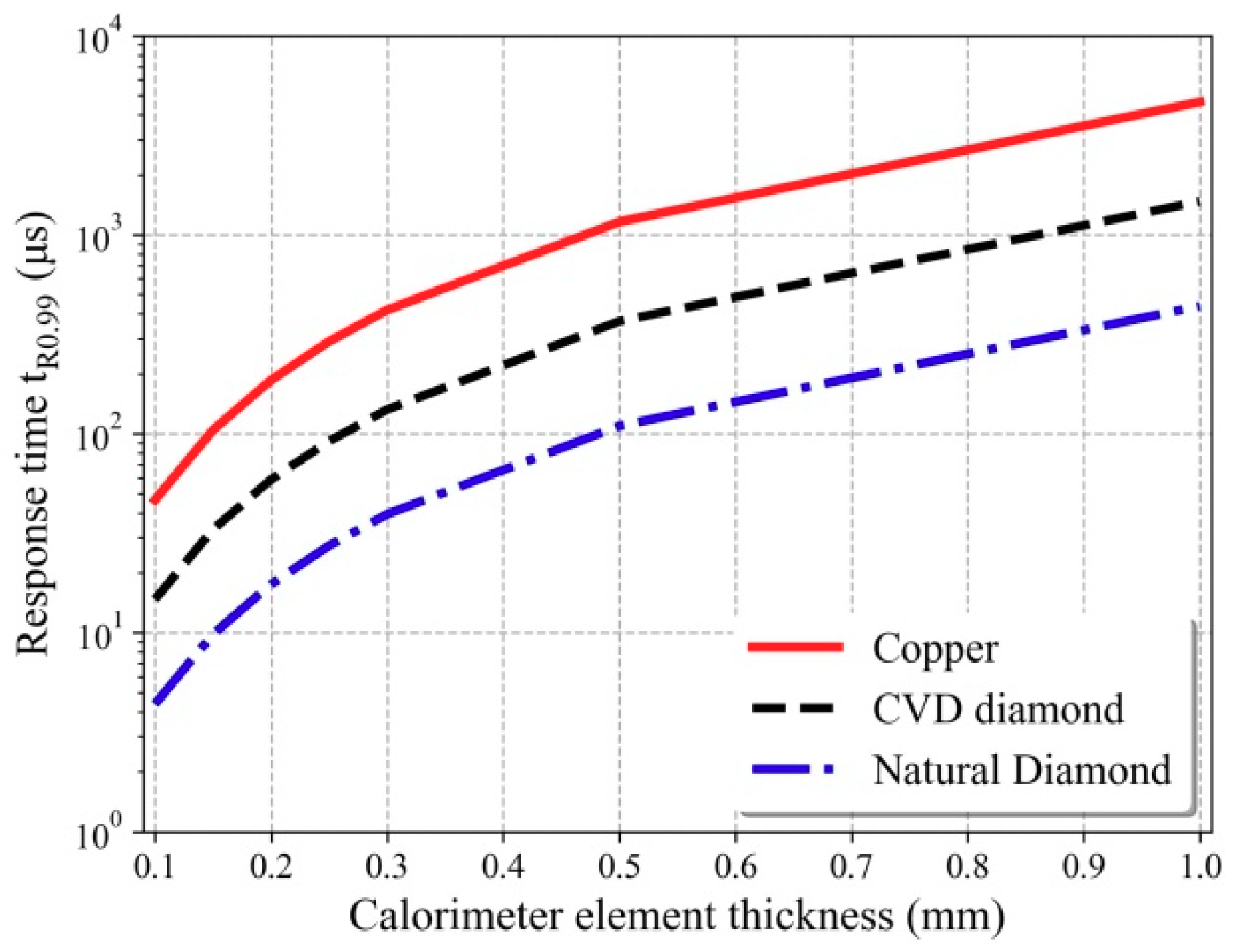
The response time tR0.99 (99%) is selected as the characteristic response time of the sensor, which means that the heat flux at the back of the calorimeter element reaches 99% of the surface heat flux loading. Figure 2 shows the relationship between the characteristic response time and the thickness of the calorimeter element. It is observed that the characteristic thermal response time of the natural diamond is the fastest at the same thickness, followed by the CVD diamond and copper. At a thickness of 0.2 mm, the characteristic response time of copper is 186 μs, whereas that of the CVD diamond is only 59 μs. Although the response time of the natural diamond is faster (21 μs at 0.2 mm), its cost is much higher. However, the CVD diamond meets the response time requirement at a relatively low cost.
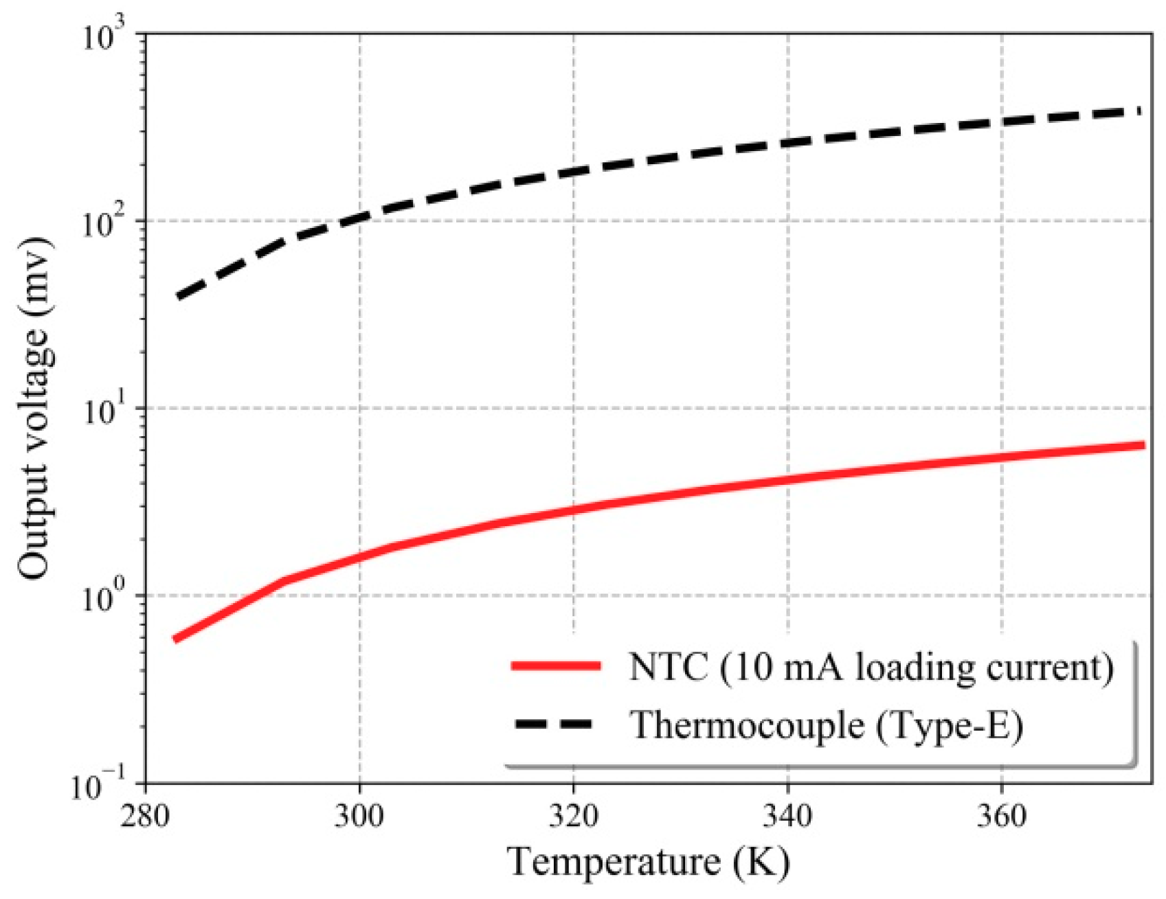
Due to the high resistivity of diamonds, the platinum film can be directly plated on the back of the calorimeter element without special insulation between them. The platinum film resistance is hidden on the back of the calorimeter element, thus protecting it from disturbances or erosion of the high-velocity gas flow. Therefore, unlike a thin-film resistance heat flux sensor, the resistance value of the NTC remains unchanged before and after the experiments, thereby ensuring the reliability and repeatability of the heat flux measurements. Additionally, the diamond element has a strong anti-erosion ability. The most significant advantage of the NTC heat flux sensor is the high signal output sensitivity compared with the coaxial thermocouple, which also has excellent response time and anti-erosion ability. The comparison of the output voltage signal versus the temperature of the NTC heat flux sensor and type-E coaxial thermocouple is shown in Figure 3. The loading current at the ends of the NTC platinum film is 10 mA. The Type-E thermocouple is commonly used for heat flux measurements in transient test facilities. The output signal of the NTC heat flux sensor is significantly higher than that of the type-E thermocouple, thereby increasing the signal-to-noise ratio and improving the accuracy.
2.2. Influence of Non-Ideal Heat Conduction
Equation (1) is applied with the assumption that the heat loss from the CVD element can be assumed to be negligible. However, the calorimeter element must be fixed and sealed during sensor manufacturing. Thus, the measurement is affected because the packaging causes heat loss of the calorimeter element, which leads to inaccuracy. Numerical simulations were conducted to understand the heat exchange between the CVD diamond and its surroundings due to the straightforward operation and detailed information. The governing equation is the axisymmetric unsteady heat conduction equation:
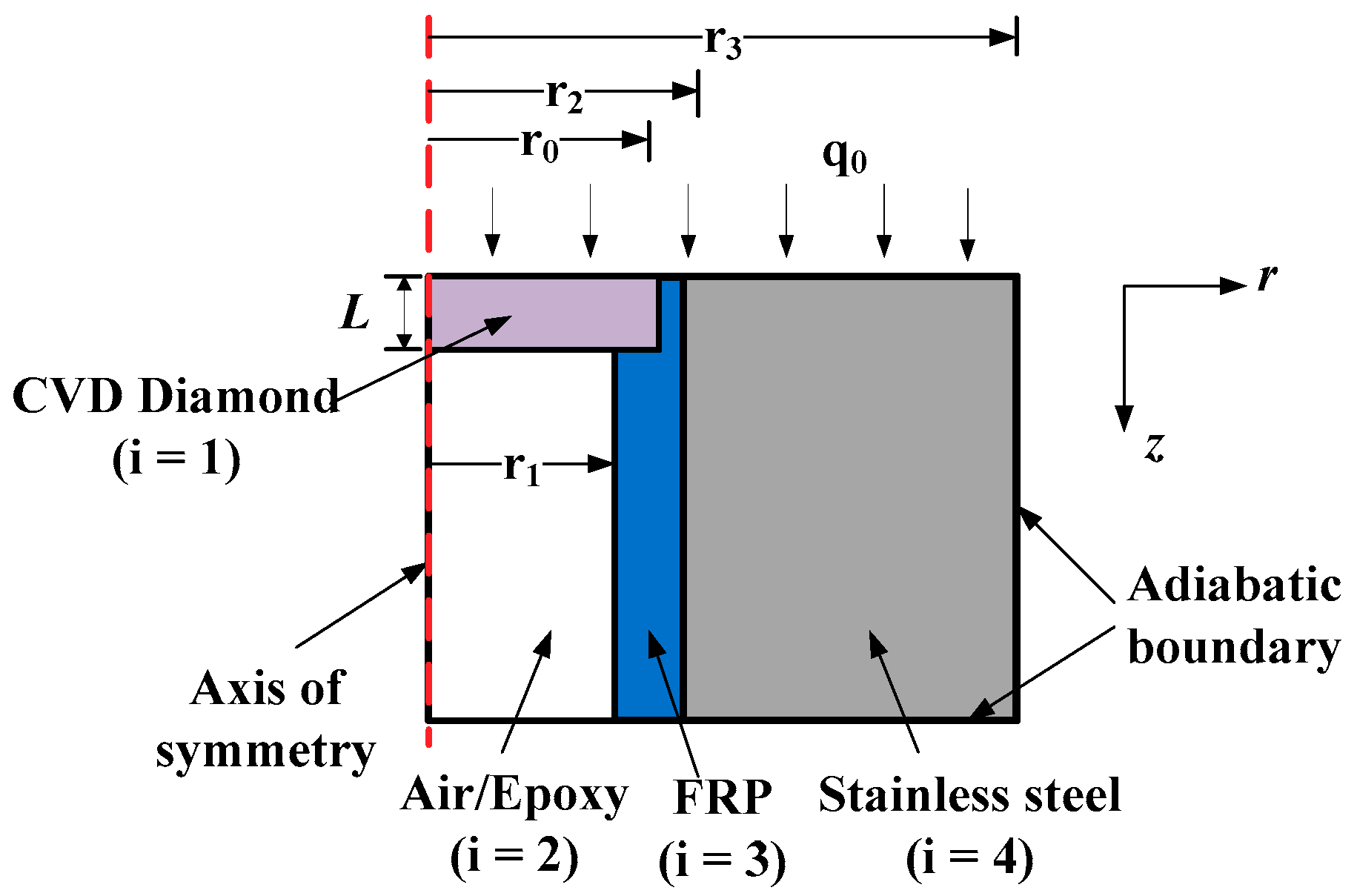
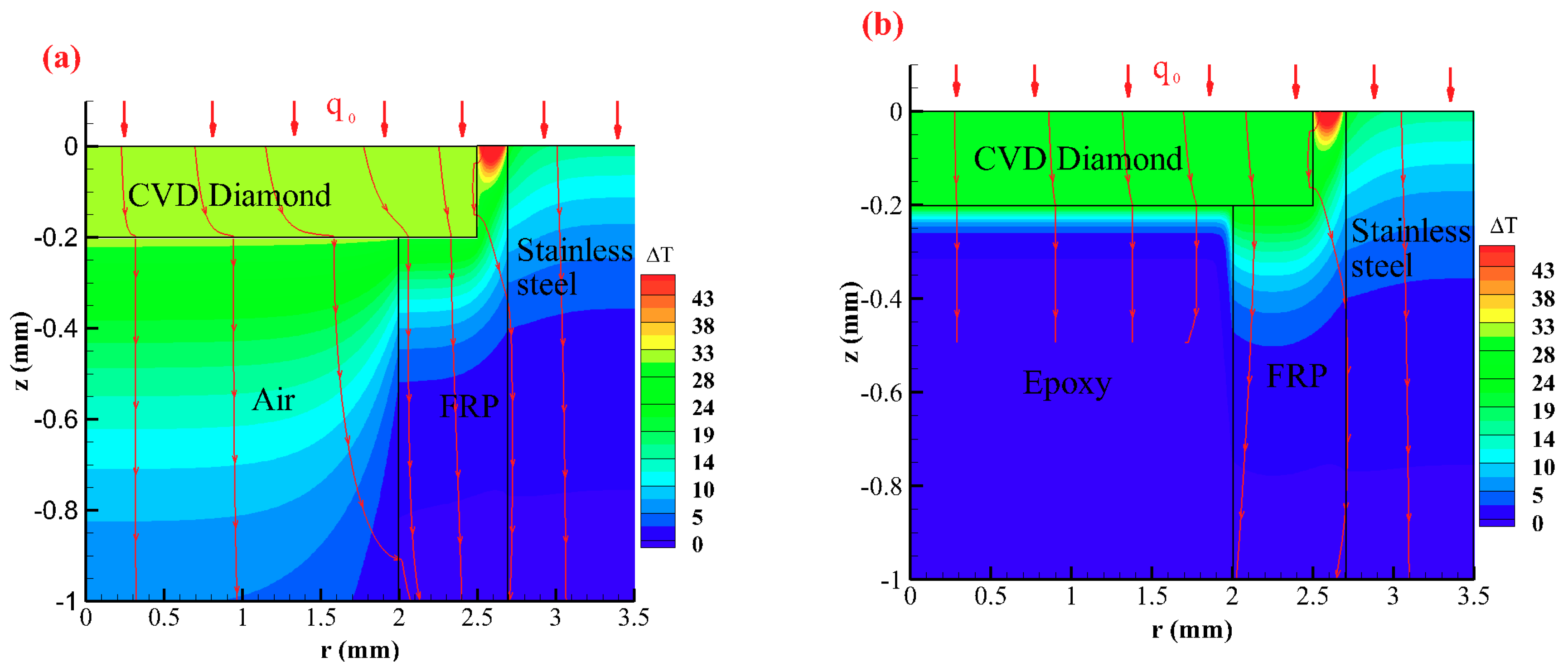
where r and z are the radial and axial directions of the calculation model, respectively; the subscripts 1, 2, 3, and 4 represent the CVD diamond, air/epoxy insulation, fiber-reinforced plastics (FRP sensor base), and stainless steel (test model), respectively, as shown in Figure 4. Equation (4) is solved using the finite difference method for spatial discretization and a fourth order Runge-Kutta method for time integration [36].
Since the thickness of the platinum film on the back of the CVD diamond is only about 0.2 μm, and the diameter of the platinum film lead line is only 0.1 mm, the heat dissipation by the platinum film and lead line on is ignored in this calculation. Due to the axial symmetry of the computational model, only half of the geometry is considered, as shown in Figure 4. In the present calculation, the CVD diamond thickness is fixed at L = 0.2 mm, which is used in the author’s home-made calorimeters; the radius is r0 = 2.5, 5 and 10 mm, respectively; the radius of the back-filling material is r1 = r0 − 0.5; the outer diameter of the FRP support is r2 = r0 + 0.2, and the outer diameter of the stainless steel model is r3 = r2 + 5.
The initial temperature of the calculation model is set to T∞ = 293 K for the calculation. A constant uniform heat flux (q0 = 1.0 MW/m2) is loaded on the top surface. Thus, the boundary conditions at the top surface are as follows:
Other boundary conditions are shown in Figure 4. In addition, the temperature and heat flux satisfy the continuity condition at the interface between the two different materials.
It also needs to be noted that the back-filling material is air or epoxy insulation, both of which have very low heat conductivity and reduce the heat loss from the CVD to its surroundings. These materials are commonly used in calorimeters, where epoxy can be used to enhance the strength of the sensor. The model material here is made of stainless steel, which is commonly used in shock tunnel experiments; and its physical parameters are shown in Table 1.
The equations were solved by our developed C++ program in this study and structured grids of 250 × 300 are applied. The zones inner the calorimeter and the calorimeter/back-filling material interface are incorporated with clustered points to provide good spatial resolution. The temperature distribution in the calculation model at different times were output during the calculation process to understand the heat transfer inside the senor. Temperature distributions were generated by the software Tecplot 360 as shown in Figure 5.
Figure 5 shows the simulated temperature distribution inside the calculation model for r0 = 2.5 mm at the moment of t = 12 ms; Figure 5a shows the results for the air as back-filling material, and Figure 5b depicts the result of using epoxy. As expected, a more complicated heat conduction process occurs around the CVD diamond. First, the temperature on the top surface of the computing model is not constant, and the smaller ρck value of the FRP results in a higher surface temperature than that of the CVD diamond and the stainless-steel model. However, air or epoxy has a lower temperature than the CVD diamond at the backside (around z = −0.2 mm in Figure 5). Thus, the thermal environment around the CVD diamond is complex; heat is absorbed laterally from the FRP at the surface region, but energy is dissipated to the bottom substrate. This result disagrees with the assumption of no heat loss from the CVD diamond element due to the different thermo-physical parameters of the CVD, FRP, air/epoxy, and the test model. However, this study did not specifically focus on the details of the thermal environment; instead, the performance of the sensor was analyzed by comparing the heat flux monitored at the back center of the CVD diamond (qb), as described by the nondimensional form of qb/q0, where the heat transfer rate q0 represents the heat flux applied to the model surface. Results for qb/q0 that are greater than one indicates larger measuring results, and vice versa. Values of qb/q0 that are closer to one indicate a smaller influence on the measurement results and vice versa.
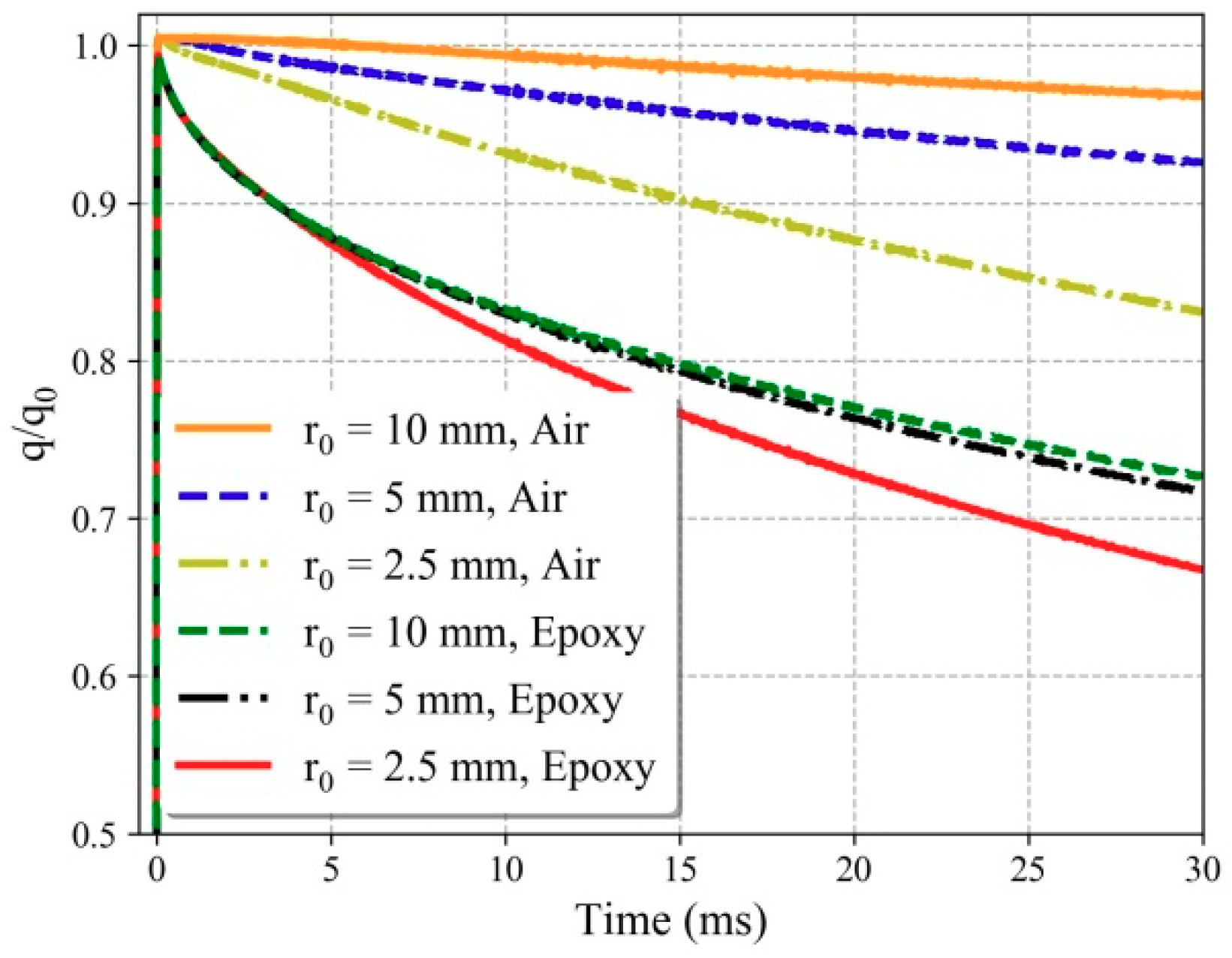
Figure 6 shows the heat flux calculation of the NTC sensor with different back-filling materials and different sensor sizes. Since the effective test time of impulse high-enthalpy faculties is usually very short, in the order of several microsecond. The discussion is mainly focused on 30 ms. For the sensor with air back-filling, the larger the sensor diameter, the larger qb/q0 is, and the smaller the influence on the heat flux measurements is. The size of the sensor with epoxy back-filling has little influence on the measurement deviation; all cases have lower values of qb/q0 than that of the air back-filling case duo the larger ρck of epoxy. For the sensor with air back-filling, at t = 30 ms, the heat flux error at the center position is 3.2% for r0 = 10 mm, and the errors are 7.4% and 16.9% for r0 = 5 mm and r0 = 2.5 mm respectively. The deviation is about 30% at t = 30 ms for all epoxy back-filling sensors. The main reason is the heat dissipation effect of the mounting base of the calorimeter. Due to the mounting structure, this measurement deviation is difficult to avoid. Unfortunately, all deviations increase with increasing time. Thus, a correction or calibration is needed to obtain high-accuracy heat transfer measurement results, especially for sensors with high ρck values.
3. Theory of Dynamic Correction
According to the numerical calculation results, the heat flux loss on the back of the calorimeter increases over time. Thus, a dynamic correction is necessary to obtain accurate measurement results. Only the heat flux loss from the bottom of the CVD diamond was considered in the present corrections, and the heat exchange in the lateral direction was ignored. However, it will become evident in the following discussion that the lateral heat exchange does not have a significant influence on the corrections.
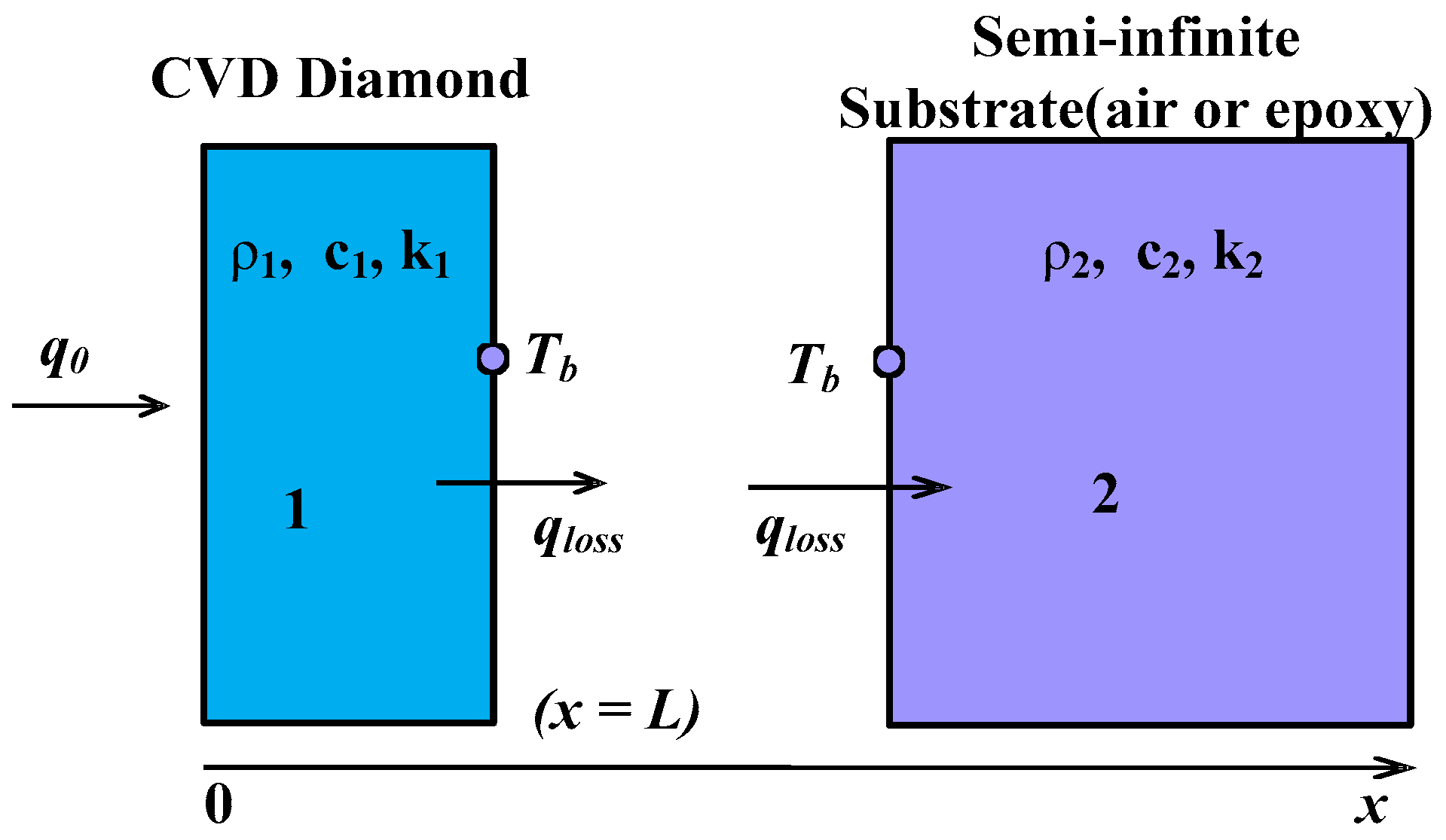
The heat dissipation effect of the back-filling material is simplified as a one-dimensional heat conduction problem of two different materials, as shown in Figure 7, where ρ1, c1, and k1 are the density, the specific heat, and the thermal conductivity of the calorimeter element (CVD diamond in the present study). ρ2, c2, and k2 are the density, the specific heat, and the thermal conductivity of the backing material (air or epoxy). According to reference [14], the calculation formula of the heat penetration depth for the lining material is as follows:
The effective test time of transient facilities is typically in the order of milliseconds. The heat penetration depth of epoxy would only be 0.4 mm at a longer test time of 100 ms. Thus, the backing material can be regarded as a one-dimensional semi-infinite body, where the surface temperature is monitored using the platinum thin-film resistance, which is labeled Tb in Figure 7.
The heat conduction equation for a two-layer semi-infinite system as shown in Figure 7 is defined as
where subscript 1 is the calorimeter element and subscript 2 is the substrate. Their boundary conditions are as follows
Thus, by taking the Laplace transforms, the temperature at the back of the calorimeter element or the surface of the substrate is obtained by solving Equations (7) and (8) [14]:
where is the ratio of the back-filling material to calorimetric element material; P is the Laplace operator. Subsequently, the heat flux loss to the substrate is obtained by and the one-dimensional semi-infinite heat conduction theory:
By combining Equations (9) and (10), the following expression is obtained using the Taylor expansion and the inverse Laplace transform:
where α1 is the thermal diffusion coefficient of the calorimeter element. Detailed processes of the above derivation can be found in [14,36].
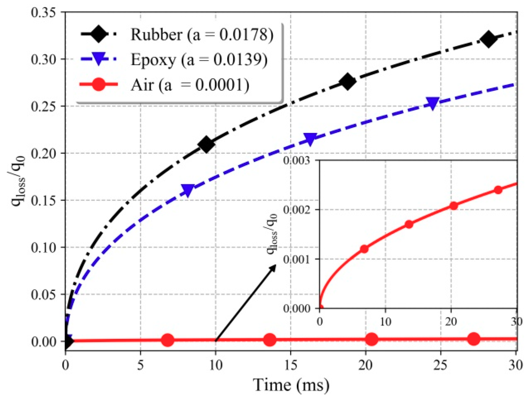
Figure 8 shows the relationship between qloss/q0 and time for three commonly used back-filling materials, where the calorimeter element is CVD diamond; its thermal diffusion coefficient can be found in Table 1. The larger the value of a, the larger the value of qloss/q0, and qloss/q0 increases over time. Of course, air is the best back-filling material of the calorimeter element, and its largest deviation is less than 0.3% (at 30 ms). However, the pressure resistance is poor when air is used as the back-filling material, which limits the application range of the sensor. This is especially the case in high-enthalpy flows, where small particles of metallic or nonmetallic materials exist. Epoxy is commonly used as a filling material for calorimeters to enhance the strength. Unfortunately, its heat flux loss is much higher than that of air, and qloss/q0 is more than 10% for a test time of 3 ms. Thus, corrections are needed if high-accuracy heat flux results are expected.
According to the energy conservation law, the loaded heat flux on the surface q0 has the following relationship with the absorbed heat flux of the CVD diamond qb and the heat flux loss to its surroundings qloss:
q0 = qb + qloss
In actuality and for simplicity, qb is the heat flux value calculated by Equation (2) from the sensor output temperature signal. Additionally, qloss is the heat flux transferred from the calorimeter element to the backing material, namely, the heat flux rate lost from the CVD diamond. qloss is calculated from Equation (11) and is brought into Equation (12). We also define the correction coefficient of the transient calorimeter as:
Then, Equation (12) can be rewritten as
where is a function of the effusivity ratio a and time t for a specific calorimeter. The dynamic correction of the calorimeter measurement results can be made using Equation (14) if the thermal diffusion coefficient of the back-filling material can be obtained.
The parameters of epoxy in the simulation in Section 2.2 can be obtained from Table 1. The dynamic correction in Equation (14) was first used to correct the simulated results. The calorimetric element radius of r0 = 2.5 mm is used as an example; the calculation result in Figure 6 was modified using Equation (14), and the results are shown in Figure 9. The error before the correction is 33% at 30 ms, and the overall error after the correction is within 7.8%. This deviation is within 2.3% if the test time is smaller than 12 ms. Although only one-dimensional heat conduction is considered in the modification, it is found that the lateral heat flux loss from the CVD diamond can be ignored. The results are considered excellent for heat flux measurements.
It is observed that the measurement error of the transient calorimeter can be reduced to acceptable deviation level after the dynamic correction (Equation (14)) since the thermal diffusivity of the backing material is known. During the manufacturing process of the sensor, the epoxy is attached to the back of the calorimetric element by potting and subsequently solidifies. However, the epoxy is a compound, and the physical parameters are difficult to determine. Meanwhile, the potting quality is difficult to maintain, and the physical parameters of the bottom lining materials are quite different in actual sensors. Therefore, it is necessary to calibrate the physical parameters of the back-filling material before applying the dynamic correction of the NTC calorimeter. Subsequently, the dynamic correction coefficient of each sensor can be obtained. Similarly, other types of sensors, such as thin-film resistance thermometers and thermocouples, need to be calibrated before application to obtain high-accuracy experimental results.
4. Experiments Results and Discussion
The above analysis provides theoretical evidence for the dynamic correction of the transient calorimeter under non-ideal conditions. Further, the correction method is verified through aerodynamic heating measurement experiments. Since the dynamic correction coefficient is related to the test time, different test time conditions were chosen to fully test the correction method and the sensor performance.
4.1. Experimental Facility
The calibration experiments were conducted in a shock tube/tunnel that uses detonation driving. The facility is located in the Laboratory of High-Temperature Gas Dynamics (LHD) at the Institute of Mechanics, Chinese Academy of Sciences, Beijing, China. A schematic of the shock tunnel is shown in Figure 10a. The system consists of a dump section, a driver section, a driven section, a hypersonic nozzle, and a test section. The dump, driver, and driven sections are 3, 15, and 11 m in length, respectively, and they have the same inner diameter of 224 mm. The test section is 10 m long and 1.2 m in diameter. The nominal Mach number of the nozzle is 5.5, and the nozzle exit diameter is 300 mm. Both the main and auxiliary diaphragms are flat-scored metal diaphragms. Different depths of the grooves are designed to ensure that they will not fail during initial pressure differences across the diaphragms before igniting the flammable gases. An ignition tube is placed close to the main diaphragm in the driver tube. The mixture in the ignition tube is initially ignited by electrical sparks. A high-temperature jet is formed and propagates into the driving section, thereby igniting the detonable gas directly. This leads to a stable detonation wave traveling upstream in the detonation tube, behind which a Taylor wave follows; the products have high temperature and pressure. Using detonation as the driving method, the facility can provide high-temperature gas conditions for hypersonic flight.
As a supplement to extend the capabilities of the facility, it can be re-arranged to operate under other types of test conditions. One is called the single detonation shock tunnel, which has a longer test time; the schematic of the facility is shown in Figure 10b. Then the main diaphragm is removed, and the detonation wave propagates to the left side as it is ignited close to the nozzle throat. The high-temperature and high-pressure gas source behind the Taylor wave are used as the experimental gas; namely, the experimental gas composition represents the detonation product. Another test condition is obtained using the detonation-driven shock tube, as shown in Figure 10c. Compared to the detonation shock tunnel (Figure 10a), the nozzle is removed, and the test model is placed at the exit of the driven section.
In the present study, we use these three types of operations to fully validate our new calorimeters. All the tests in the present study were conducted at room temperature. The measurement system used in this experiment mainly include a conditioner and a data acquisition board, which are integrated into an equipment by Donghua software, INC (Taizhou, Jiangsu, China). Before the experiment, a constant of 10 mA current provided by the conditioner was loaded on each sensor. The voltage at the ends the platinum film resistance were also amplified by the conditioner at a gain factor of 100. All signals from the sensors were acquired by the data acquisition board and were processed on a PC-based data acquisition system at a sampling rate of 1 MHz. The measured voltage signals were converted into temperature signal according to the temperature coefficient of the sensors which had been statically calibrated before the experiment. Besides, the measurement system was also calibrated and the overall measurement deviation was found to be 0.15%. The other details of the facility, the pressure/incident shock speed measurement method or position, and the free-stream parameter calculation method are available in reference [36].
4.2. Test Model and Sensor Arrangement
For the comparative experiments, two types of NTC sensors are designed in the present study. One has a radius of 10 mm and a back-filling material of air (NTC-10), and the other miniaturized sensor has a radius of 2.5 mm and a bottom liner filled with epoxy (NTC-2.5). Figure 6 shows that the sensor NTC-10 obtains excellent heat flux results even without corrections. However, the epoxy in the sensor NTC-2.5 leads to heat flux dissipation so that dynamic corrections are necessary. It should be noted that the radius used here represents the dimension of the CVD diamond, and the radius of the entire sensor is 0.2 mm larger, i.e., 10.2 and 2.7 mm for the NTC-10 and NTC-2.5, respectively.
Two types of typical models were selected in the present study, a flat plate and an R20 sphere. The flat plate was used in the shock tunnel, and the sphere was used in the shock tube. The flat plate, which is a 17° angle wedge model, is shown in Figure 11. In this design, the flat plate on the wedge model can be replaced. Due to the relatively large size of the NTC-10, two flat plates are designed. In flat plate 1, three NTC-10 sensors (No. C01–C03) are evenly installed at 150, 200, and 250 mm from the apex along the axis. In flat plate 2, three NTC-2.5 sensors (No. C04–C06) are installed at the corresponding positions. On both sides of C05, two NTC-2.5 sensors (No. C07, C08) are installed at a distance of 50 mm. In addition, there are two reasons for the choice of the plate model; one is that the sensor can be installed flush with the model to reduce measurement errors caused by the installation deviation, especially for the larger NTC-10 sensor. The other reason is that the heat flux of the plate model can be obtained theoretically.
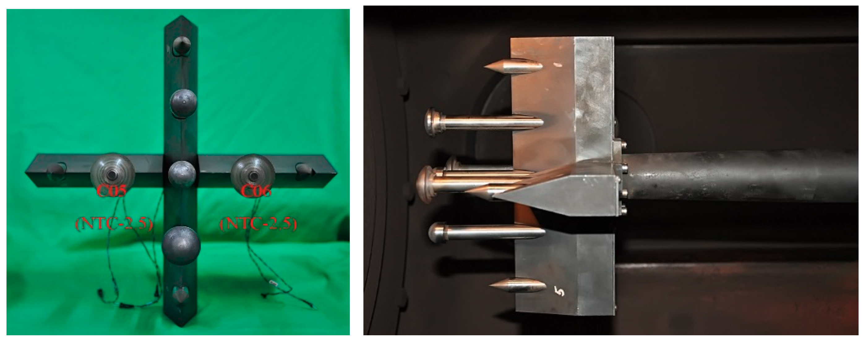
For the R20 mm sphere model, only two NTC-2.5 calorimeters (No. C05–C06) were installed, as shown in Figure 12. The test model was placed 50 mm downstream of the open end of the driven tube to avoid disturbances caused by the interaction between the detached shock wave and the inside wall of the tube to the flow field around the test model.
4.3. Results and Discussion
4.3.1. Results of the Detonation Shock Tunnel Test
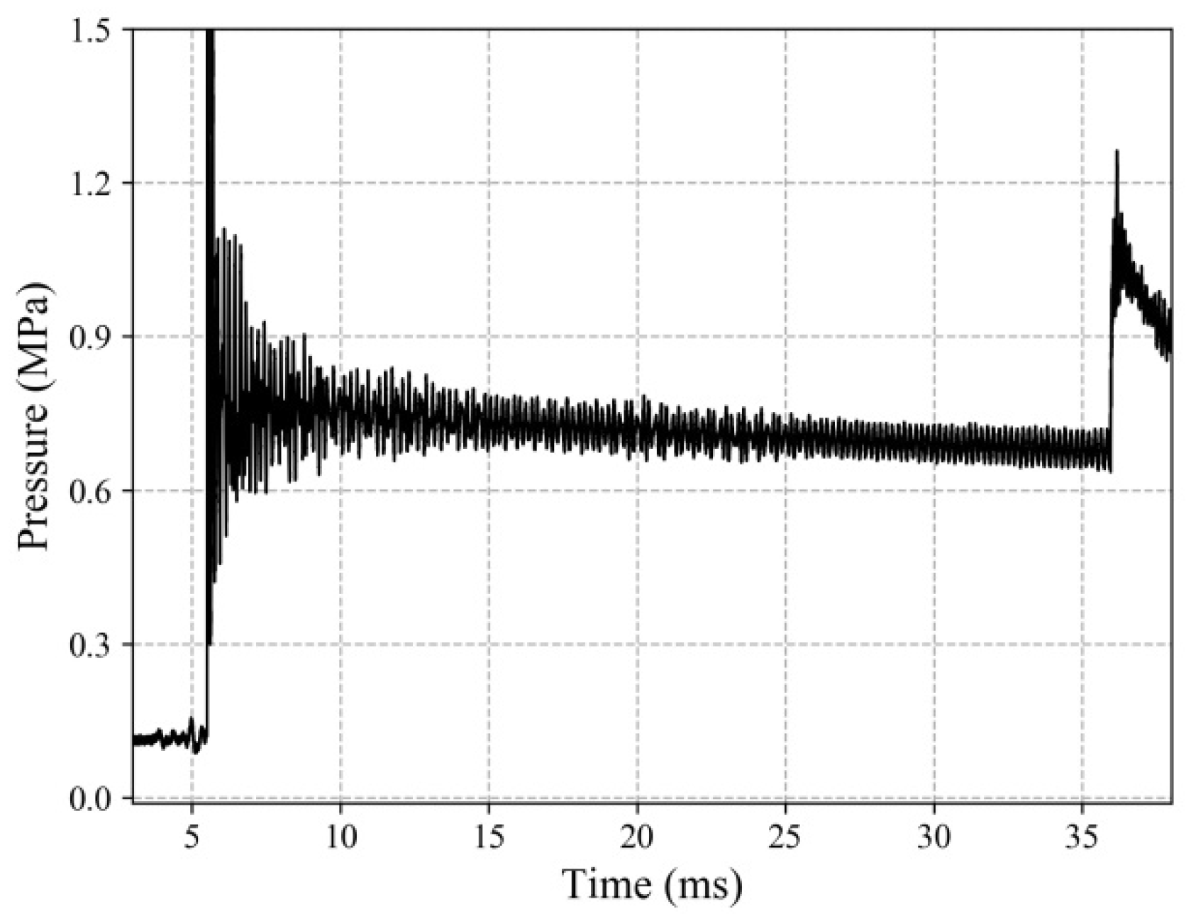
In the detonation shock tunnel, a mixture of 2H2 + O2 + 2N2 was used as the initial driver gas, and air was used as the initial test gas in the driven section. The initial pressure values were 0.27 MPa and 3800 Pa, respectively. The test parameters are listed in Table 2; the total pressure was 1.22 MPa, and the temperature was 3570 K. The reservoir pressure was measured using pressure transducers mounted at the end of the shock tube. The other reservoir parameters were computed using the measured shock tube filling pressure, shock speed, and nozzle reservoir pressure. The stagnation pressure history is shown in Figure 13. The plateau pressure is maintained for about 14 ms. Based on the reservoir conditions, the free-stream was subsequently determined by numerically rebuilding the nozzle flow [37].
Figure 14 shows the temperature curve obtained from the NTC-10 in flat plate 1 and the corresponding calculated heat flux curve. As shown in Figure 14b, the variation of the heat flux over time reflects the stages of flow field starting and stability processes. The heat flux is relatively stable during the effective test time, and the steady flow duration lasts about 14 ms.
Since the free-stream flow parameters are known (Table 2), the surface heat flux of the flat plate can be obtained theoretically. The reference enthalpy method [38] is used to calculate the theoretical heat flux:
where ρ*, μ* are the gas parameters corresponding to the reference temperature; haw is the adiabatic wall enthalpy, namely the recovery enthalpy; hw is the wall enthalpy; ρe, μe are the incoming flow parameters from the outer edge of the boundary layer, i.e., the gas parameters after the oblique shock wave for the wedge model.
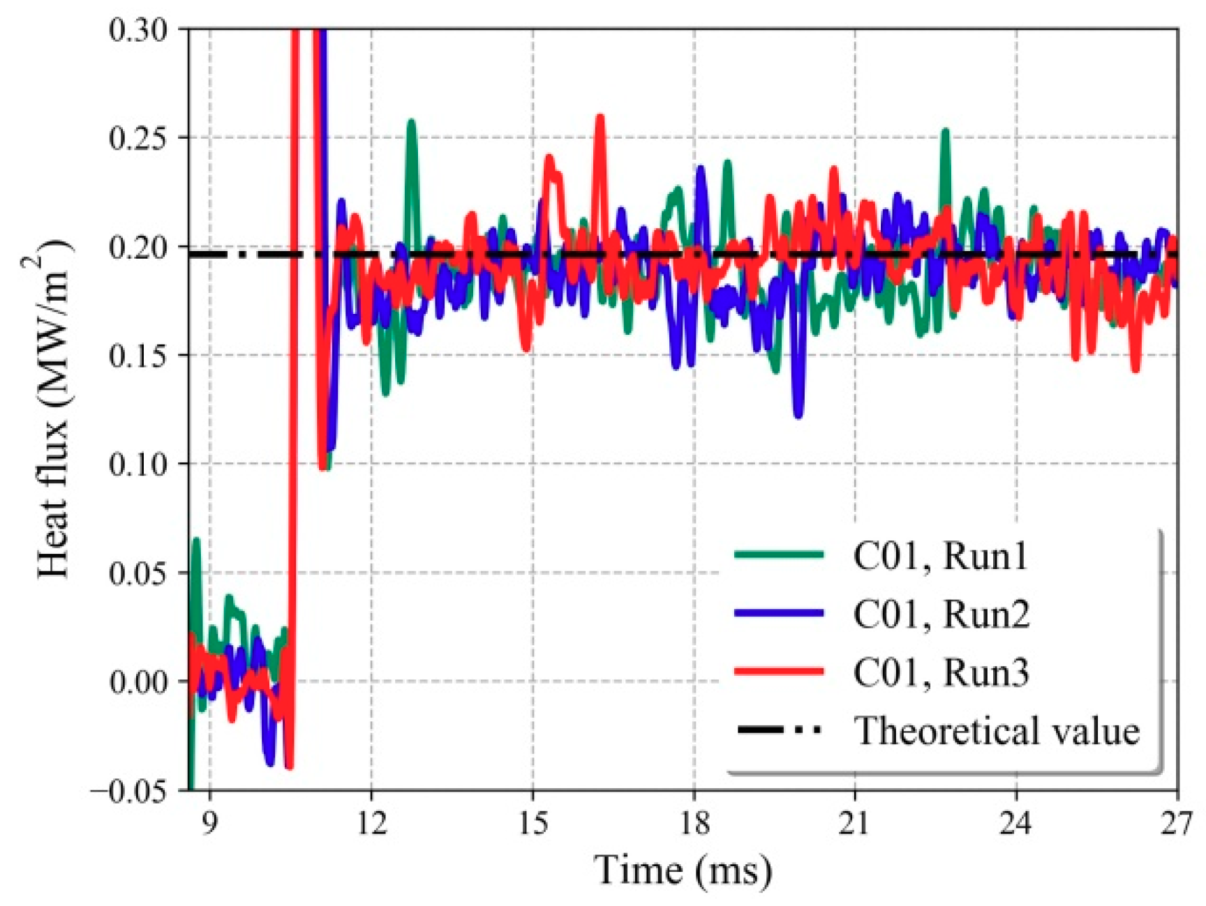
The repeatability of the experiments and the measurements was investigated. Figure 15 shows the obtained heat flux histories of C01 (NTC-10) for three measurements for the same nominal test conditions. The value between 15 ms and 25 ms in Figure 15 is used as the experimental heat flux. The relative standard deviation of the heat flux in the three tests is about 1.7%. The average heat flux amounts to 0.192 MW/m2. Table 3 summarizes the results of heat flux values obtained from the three NTC-10 sensors and the theoretical value. The experimental value is slightly lower than the theoretical value, which is due to the heat flux loss from the CVD diamond. The measurement deviations between the experimental and theoretical values are within 6%, and the relative standard deviations of all sensors are within 2%. Thus, the results show that the NTC sensor with air as a backing material provides acceptable results even without corrections, and the results correspond to the simulated results, as shown in Figure 6.
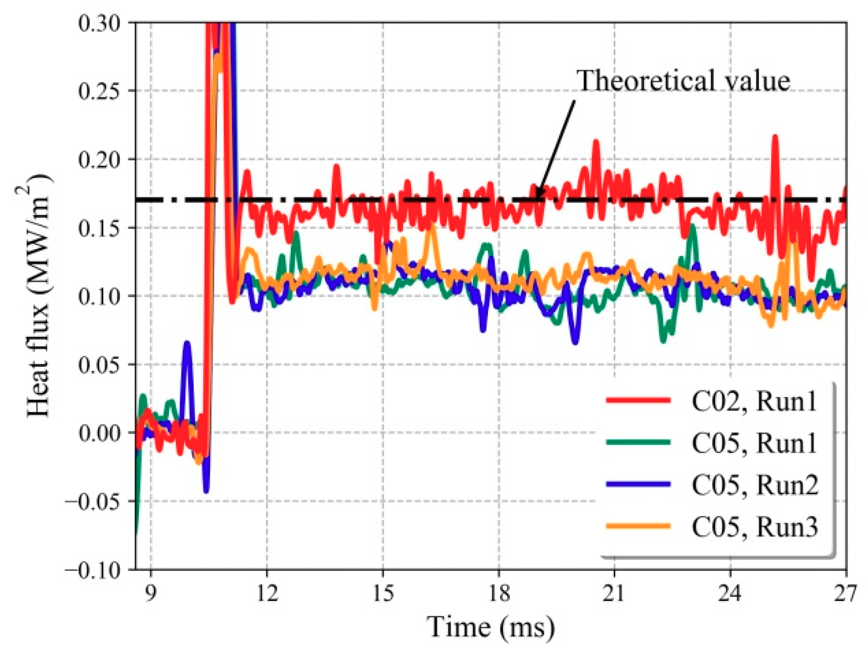
Figure 16 shows the comparison of the three heat flux measurement results of the sensor C05 (NTC-2.5) in plate 2, and the sensor C02 (NTC-10) at the same position in plate 1. The results of the NTC-2.5 sensor are about 30% lower than the theoretical value. This result is expected, since the epoxy in the NTC-2.5 absorbs a considerable amount of energy from the CVD diamond, resulting in deviations, as calculated in Section 2.2. However, the repeatability of the NTC-2.5 sensor is also very good.
The corrections of the results of the NTC-2.5 in Figure 16 are performed using Equation (14). However, the ρck value of the epoxy needs to be obtained. Since the physical parameter of the epoxy has large deviations due to the manufacturing processes, the ρck of the epoxy in the present sensors is calibrated using a comparison to the theoretical heat values instead of using the data in Table 1. Different ρck values of the epoxy are tested in Equation (14) to correct the results of the NTC-2.5 sensors; the ρck value that achieves the best agreement between the corrected and theoretical values is used. Figure 17 shows the heat flux curves of C05 (NTC-2.5) with/without corrections. The corrected result agrees well with the experimental results and the results of the C02 (NTC-10) sensor. The ρck values of epoxy for the five NTC-2.5 sensors are shown in Table 4; the relative standard deviation between the values is about 11%, which is attributed to an error in the production process. Although this deviation may be improved, a calibration of each sensor is needed if high accuracy heat transfer measurements are desired. This applies also to other sensors since the ρck values of Type-E thermocouples also require detailed calibration.
4.3.2. Results of the Single Detonation Shock Tunnel Test
For the validation of the proposed NTC sensors, the flat plate with the two types of NTC sensors was tested in the single detonation shock tunnel, where the test time is much longer than that of the detonation shock tunnel. The detonation section was filled with a mixture of 2H2 + O2 + 1.25N2 at a pressure of 0.12 MPa. The total pressure was about 0.725 MPa, and the temperature was about 2862 K. The stagnation pressure history is shown in Figure 18 for a test time of about 30 ms. Six experimental runs were conducted in the single detonation operation mode, with three test runs for plates 1 and 2, respectively. The sensor installations were the same as those in the detonation shock tunnel experiments. The free-stream parameters are not displayed here since theoretical methods are not available to obtain the heat flux on the flat plate for the combustion products of 2H2 + O2 + 1.25N2.
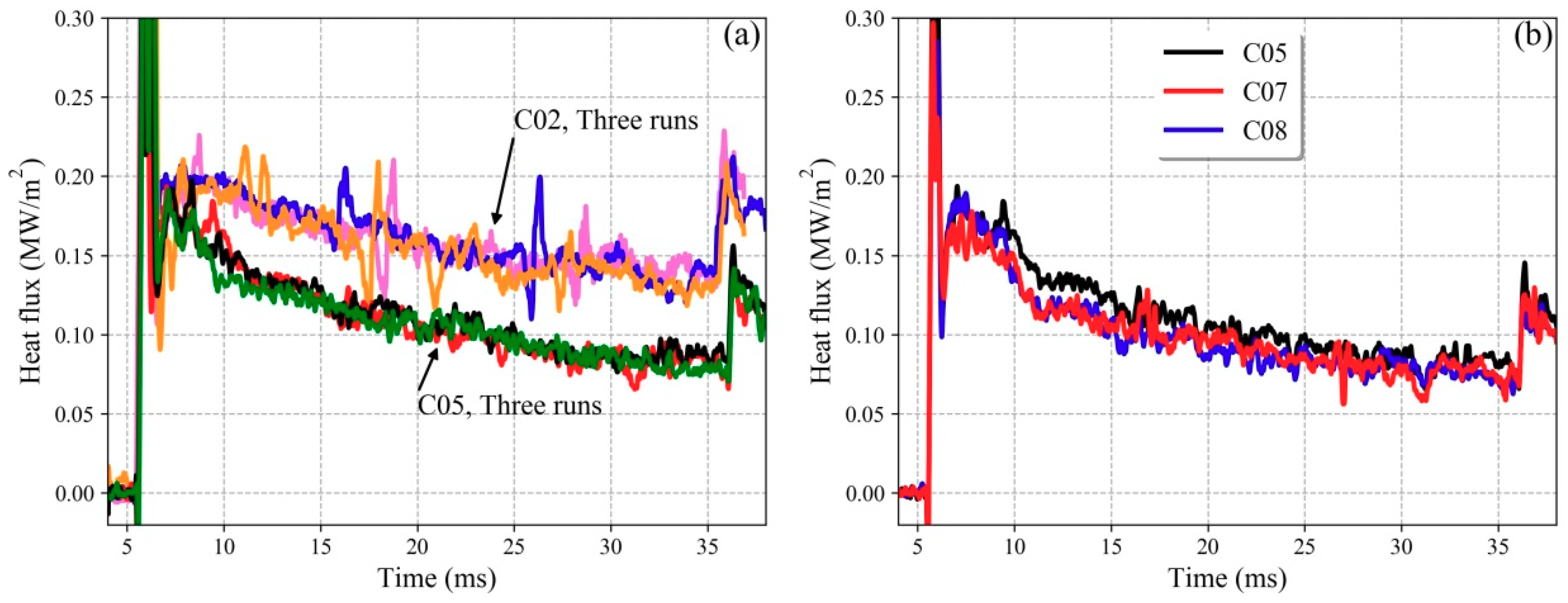
Figure 19 shows the heat flux curves of NTC-10 and NTC-2.5. Both sensors underwent three test runs. The repeatability of both sensors is good. The heat flux curve of NTC-10 shows a downward trend with time, which is attributed to the continuous decrease in stagnation pressure, as shown in Figure 18, rather than a sensor problem. Besides, the heat flux obtained from the NTC-2.5 is smaller than that of the NTC-10 and shows the same regularity, as shown in Figure 16, in the detonation shock tunnel experiments. This result is attributed to the much greater heat loss from the CVD diamond to the epoxy than to the air. Since the test time is much longer in the single detonation shock tunnel, it is obvious to find that the difference between these two sensors increases over time, which also corresponds with the simulated results shown in Figure 6.
Subsequently, the heat flux curve of C05 in Figure 19 is corrected by Equation (14), and the results are shown in Figure 20. It should be noted here that the value of a is the value obtained from the results in Section 4.3.1. The corrected/uncorrected results of C05 are shown in Figure 20. The corrected results of C05 agree well with the heat flux of C02, which has a small deviation from the real heat flux loading, as discussed in Section 4.3.1. Thus, the dynamic correction method for the NTC sensors shows good performance, even for a test duration as long as 30 ms.
4.3.3. Results of the Detonation Shock Tube Test
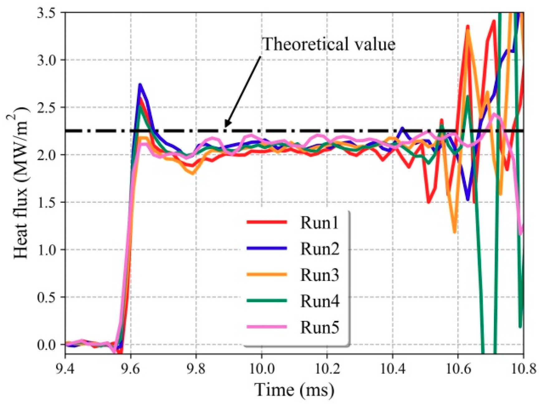
Since the shock tube allows for more quantitative studies than the other tests and the free-stream flows can be accurately obtained through the shock tube theory, the calibration of the sensors was also conducted using the detonation shock tube. However, the test time in the shock tube is much shorter than that of the other tests. Due to the test space limitation of the shock tube, only two NTC-2.5 sensors (C05 and C06) were installed on two R20 spheres; the sensor arrangement is shown in Figure 12. Five tests were conducted. The measured heat flux curves for C05 are shown in Figure 21, where the heat flux of NTC-2.5 is corrected in the same manner as described in Section 4.3.2. However, since the test time was less than 1 ms, the corrections were also very limited, and the discrepancy was 6% at most, as shown in Figure 8. The heat flux curves show excellent repeatability, similar to the other tests.
The value between 9.8 and 10.4 ms in Figure 21 is used as the experimental heat flux. The heat flux results are summarized in Table 5, including the theoretical results obtained using the Fay-Riddle formula and the test flow in the shock tube. According to the Fay-Riddle formula, the heat flux at the stagnation point is [39]:
Here ρ, μ, and h are the gas density, viscosity, and enthalpy, respectively, and Pr is the Prandtl number. The subscripts w and e denote the conditions at the wall and the outer edge of the boundary layer, respectively. (du/dx)0 is the velocity gradient at the outer edge of the boundary layer. The subscripts 1 and 2 in Table 5 denote the test gas in front and behind the incident shock wave, respectively. Ms is the incident shock Mach number. The experiment in the detonation shock tube was conducted under the following conditions: a mixture of 2H2 + O2 + 1.5N2 and a pressure of 0.08 MPa in the driving section. The shock tube was filled with air at a pressure of 5000 Pa.
It is observed that the measured heat fluxes with corrections are, on average, 7.5% lower than the theoretical results, and the maximum deviation is 10.1%. The main reason is that the sensor is too large for the spherical model; the curvature of the stagnation point is changed, resulting in lower heat flux. Nevertheless, the overall repeatability is excellent, and sensors with smaller size are being developed to obtain the heat flux at a location with small curvature.
5. Conclusions
In this study, we examined the measurement performance of a robust fast-response transient calorimeter by solving the two-dimensional heat conduction equation and conducting verification tests in a transient facility with three test conditions to fully validate the new calorimeters. The following conclusions were drawn from the experimental and numerical results. First, the non-ideal thermal environment of the NTC calorimeter (heat exchange with the surroundings) resulted in a smaller measured heat flux than the loaded heat flux. The larger the effective thermal effusivity of the back-filling material, the larger the heat energy loss from the CVD diamond was, and the larger the measurement deviation was. Accordingly, a dynamic correction method was developed to compensate for the energy loss from the backside of the calorimeter element. Finally, the experimental results of the NTC calorimeters in the transient facilities exhibited good repeatability, and the corrected results of the NTC-2.5 sensors showed good agreement with the theoretical heat flux.
Currently, work in this area is still in progress, and additional experimental studies using different sensor diameters and different back-filling materials are necessary for demonstrating and improving the construction technique. However, the preliminary results are encouraging, and the NTC gauges can be used to extend and supplement heat transfer measurements made by other techniques.
Author Contributions
H.C. conceived and designed the research. S.Z. and Q.W. wrote the original manuscript. J.L. and X.Z. reviewed and edited the manuscript; All authors have read and agreed to the published version of the manuscript.
Funding
This research was funded the National Natural Science Foundation of China (Grant No. 11402275 and 11902328).
Acknowledgments
We thank Hongru Yu for his advice in the experimental work.
Conflicts of Interest
The authors declare no conflict of interest.
References
- Wang, Q.; Li, J.P.; Zhao, W.; Jiang, Z.L. Comparative study on aerodynamic heating under perfect and nonequilibrium hypersonic flows. Sci. Chin. Phys. Mech. Astron. 2016, 59, 624701. [Google Scholar] [CrossRef] [Green Version]
- Peng, Z.Y.; Shi, Y.L.; Gong, H.M.; Li, Z.H.; Luo, Y.C. Hypersonic aeroheating prediction technique and its trend of development. Acta Aeron. Astronaut. Sin. 2015, 36, 325–345. [Google Scholar]
- Gai, S.L.; Nudford, N.R. Stagnation point heat flux in hypersonic high enthalpy flows. Shock Waves 1992, 2, 43–47. [Google Scholar] [CrossRef]
- Hanamitsu, A.; Kishimoto, T.; Bito, H. High enthalpy flow computation and experiment around the simple bodies. Spec. Publ. Natl. Aerosp. Lab. 1996, 29, 10–16. [Google Scholar]
- Miller, C.G.I. Comparison of Thin Film Resistance Heat Transfer Gauges with Thin-Skin Transient Calorimeter Gauges in Conventional HW Tunnels; NASA Technical Reports Server: Hampton, VA, USA, 1982.
- Wannenwetsch, G.; Ticatch, L.; Kidd, C.; Arterbury, R. Measurements of wing leading edge heating rates on wind tunnel models using the thin film techniques. In Proceedings of the 20th Thermophysics Conference, Williamsburg, VA, USA, 19–21 June 1985; AIAA: Williamsburg, VA, USA, 1985. [Google Scholar]
- Saito, T.; Kuribayashi, T.; Menzes, V.; Sun, M.; Jagadeesh, G.; Takayama, K. Unsteady convective surface heat flux measurements on a cylinder for CFD code validation studies. Shock Waves 2004, 13, 327–337. [Google Scholar] [CrossRef]
- Saravanan, S.; Jagadeesh, G.; Reddy, K.P.J. Convective heat transfer rate distribution over a missile shaped body flying at hypersonic speeds. Exp. Fluid Sci. 2009, 33, 782–790. [Google Scholar] [CrossRef]
- Sanderson, S.R.; Sturtevant, B. Transient heat flux measurement using a surface junction thermocouple. Rev. Sci. Instrum. 2002, 73, 2781–2787. [Google Scholar] [CrossRef] [Green Version]
- Menezes, V.; Bhat, S. A coaxial thermocouple for shock tunnel applications. Rev. Sci. Instrum. 2010, 81, 104905. [Google Scholar] [CrossRef]
- Mohammed, H.A.; Salleh, H.; Yusoff, M.Z.; Campo, A. Thermal product of type-E fast response temperature sensors. J. Sci. 2010, 19, 364–371. [Google Scholar] [CrossRef]
- Desikan, S.L.N.; Suresh, K.; Srinivasan, K.; Raveendran, P.G. Fast response coaxial thermocouple for short duration impulse facilities. Appl. Eng. 2016, 96, 48–56. [Google Scholar]
- Mohammed, H.; Salleh, H.; Yusoff, M.Z. Design and fabrication of coaxial surface junction thermocouples for transient heat transfer measurements. Int. Commun. Heat Mass Transf. 2008, 35, 853–859. [Google Scholar] [CrossRef]
- Schultz, D.L.; Jones, T.V. Heat Transfer Measurements in Short Duration Hypersonic Facilities; Technical Report AGARD-AG-165; North Atlantic Treaty Organization, Advisory Group for Aerospace Research and Development: London, UK, 1973. [Google Scholar]
- Rose, P.H. Development of the calorimeter heat transfer gauge for use in shock tubes. Rev. Sci. Instrum. 1958, 29, 557–564. [Google Scholar] [CrossRef]
- Taler, J. Theory of transient experimental techniques for surface heat transfer. Int. J. Heat Mass Transf. 1996, 39, 3733–3748. [Google Scholar] [CrossRef]
- Wool, M.R.; Murphy, A.J.; Rindal, R.A. Calorimeter measurement of heat transfer at hypersonic conditions. J. Spacecr. Rocket. 1974, 11, 363–367. [Google Scholar] [CrossRef]
- Nakakita, K.; Osafune, T.; Asai, K. Global heat transfer measurement in a hypersonic shock tunnel using temperature sensitive paint. In Proceedings of the 41st AIAA Aerospace Sciences Meeting and Exhibit, Reno, NV, USA, 6–9 January 2003. AIAA-2003-0743. [Google Scholar]
- Nagai, H.; Ohmi, S.; Asai, K.; Nakakita, K. Effect of temperature-sensitive-paint thickness on global heat transfer measurement in hypersonic flow. J. Heat Transf. 2008, 22, 373–381. [Google Scholar] [CrossRef]
- Merski, N.R. Reduction of analysis of phosphor thermography data with the IHEAT software package. In Proceedings of the 36th AIAA Aerospace Sciences Meeting and Exhibit, Reno, NV, USA, 12–15 January 1998. AIAA-1998-0712. [Google Scholar]
- Merski, N.R. Global aero-heating wind tunnel measurements using improved two-color phosphor thermography methods. J. Heat Transf. 1999, 36, 160–170. [Google Scholar]
- Wu, S.; Shu, Y.H.; Li, J.P.; Yu, H.R. An integral heat flux sensor with high spatial and temporal resolutions. Chin. Sci. Bull. 2014, 59, 3484–3489. [Google Scholar] [CrossRef] [Green Version]
- Simmons, J.M. Measurement techniques in high-enthalpy hypersonic facilities. Exp. Fluid Sci. 1995, 10, 454–469. [Google Scholar] [CrossRef]
- Buttsworth, D.R. Assessment of effective thermal product of surface junction thermocouples on millisecond and microsecond time scales. Exp. Fluid Sci. 2001, 25, 409–420. [Google Scholar] [CrossRef] [Green Version]
- NIST. ITS-90 Table for Type E Thermocouple Database. Available online: https://srdata.nist.gov/its90/download/type_e.tab (accessed on 30 July 2020).
- Marrone, P.; Hartunian, R. Thin-Film Thermometer Measurements in Partially Ionized Shock-Tube Flows. Phys. Fluids 1959, 2, 719–721. [Google Scholar] [CrossRef]
- Nawaz, A.; Santos, J.A. Assessing calorimeter evaluation methods in convective and radiative heat flux environment. In Proceedings of the 10th AIAA/ASME Joint Thermophysics and Heat Transfer Conference, Chicago, IL, USA, 28 June 2010–1 July 2010. AIAA-2010-4905. [Google Scholar]
- Santos, J.; Oishi, T.; Martinez, E. Null point calorimeter sweeps with comparisons to thermal FEA model predictions. In Proceedings of the 41st AIAA Thermophysics Conference, San Antonio, TX, USA, 22–25 June 2009. AIAA-2009-3758. [Google Scholar]
- Lohle, S.; Battaglia, J.L.; Jullien, P.; Ootegem, B.V.; Lasserre, J.P.; Couzi, J. Improvement of high heat flux measurement using a null-point calorimeter. J. Spacecr. Rocket. 2008, 45, 76–81. [Google Scholar] [CrossRef]
- Ledford, R.L.; Smotherman, W.E.; Kidd, C.T. Recent Developments in Heat-Transfer-Rate, Pressure, and Force Measurements for Hot-Shot Tunnels. IEEE Trans. Aerosp. Electron. Syst. 1968, 2, 202–209. [Google Scholar] [CrossRef]
- Yan, X.; Wei, J.; Guo, J.; Hua, C.; Liu, J.; Chen, L.; Hei, L.; Li, C. Mechanism of graphitization and optical degradation of CVD diamond films by rapid heating treatment. Diam. Relat. Mater. 2017, 73, 39–46. [Google Scholar] [CrossRef]
- Geraets, R.T.P.; Mcgilvray, M.; Doherty, L.; Morgan, R.G.; Vella, S. Development of a Fast-Response Calorimeter Gauge for Hypersonic Ground Testing. In Proceedings of the 33rd AIAA Aerodynamic Measurement Technology and Ground Testing Conference, Denver, Colorado, CO, USA, 5–9 June 2017. [Google Scholar]
- Zhang, S.Z.; Li, J.P.; Zhang, X.Y.; Chen, H.; Yu, H.R. Development of a novel transient calorimeter. Sci. Sin. Technol. 2018, 48, 1. [Google Scholar] [CrossRef] [Green Version]
- Hightower, T.M.; Olivares, R.A.; Philippidis, D. Thermal Capacitance (Slug) Calorimeter Theory Including Heat Losses and Other Decaying Processes. In Proceedings of the Thermal amp; Fluids Analysis Workshop 2008, San Jose, CA, USA, 18–22 August 2008. [Google Scholar]
- Hoffmann, K.A.; Chiang, S.T. Computational Fluid Dynamics, 4th ed.; Engineering Education System: Wichita, Kansas, KS, USA, 2000. [Google Scholar]
- Zhang, S.Z. Novel Transient Calorimetric Heat Flux Sensor. Ph.D. Thesis, University of Chinese Academy of Sciences, Beijing, China, 2018. [Google Scholar]
- Zeng, M. Numerical Rebuilding of Free-Stream Measurement and Analysis of Nonequilibrium Effects in High Enthalpy Tunnel. Ph.D. Thesis, Graduate School of the Chinese Academy of Sciences, Beijing, China, 2007. [Google Scholar]
- Eckert, E.R.G. Engineering relations for heat transfer and friction in high-velocity laminar and turbulent boundary-layer flow over surfaces with constant pressure and temperature. Trans. ASME 1956, 78, 1273–1283. [Google Scholar]
- Fay, J.; Riddell, F. Theory of Stagnation Point Heat Transfer in Dissociated Air. J. Aerosp. Sci. 1958, 25, 73–85. [Google Scholar] [CrossRef]
Figure 1.
Structural diagram of the NTC heat flux sensor (not to scale).

Figure 2.
Thermal response time versus the thickness of the calorimeter element.

Figure 3.
Output voltage of the NTC and Type-E thermocouple sensors.

Figure 4.
Schematic drawing of the simulated model (not to scale).

Figure 5.
The simulated temperature distribution (t = 12 ms, r0 = 2.5 mm). (a) Air backing; (b) epoxy backing.
Figure 5.
The simulated temperature distribution (t = 12 ms, r0 = 2.5 mm). (a) Air backing; (b) epoxy backing.

Figure 6.
qb/q0 versus time for different radii of the CVD diamond.

Figure 7.
The simplified one-dimensional heat transfer model between the calorimeter element and the back-filling material.
Figure 7.
The simplified one-dimensional heat transfer model between the calorimeter element and the back-filling material.

Figure 8.
qloss/q0 versus time based on Equation (11) for three different back-filling materials.

Figure 9.
Corrections of the calorimeter. (a) The corrected results (r0 = 2.5 mm); (b) The relative error before and after corrections.
Figure 9.
Corrections of the calorimeter. (a) The corrected results (r0 = 2.5 mm); (b) The relative error before and after corrections.

Figure 10.
Schematic diagram of the experimental facility. (a) Detonation-driven shock tunnel; (b) Single detonation shock tunnel; (c) Detonation-driven shock tube.
Figure 10.
Schematic diagram of the experimental facility. (a) Detonation-driven shock tunnel; (b) Single detonation shock tunnel; (c) Detonation-driven shock tube.


Figure 11.
Test model and sensor configuration (units in mm). (a) Plate 1 with three NTC-10 sensors; (b) Plate 2 with five NTC-2.5 sensors; (c) the 17° angle wedge model; (d) photo of the NTC-10; (e) photo of the NTC-2.5.
Figure 11.
Test model and sensor configuration (units in mm). (a) Plate 1 with three NTC-10 sensors; (b) Plate 2 with five NTC-2.5 sensors; (c) the 17° angle wedge model; (d) photo of the NTC-10; (e) photo of the NTC-2.5.

Figure 12.
Test model installation of the R20 sphere in the shock tube.

Figure 13.
Stagnation pressure histories of the detonation shock tunnel.

Figure 14.
Temperature and heat flux curves of three NTC-10 sensors in run 3. (a) Temperature curves; (b) Heat flux curves.
Figure 14.
Temperature and heat flux curves of three NTC-10 sensors in run 3. (a) Temperature curves; (b) Heat flux curves.

Figure 15.
Heat flux curves of repeated experiments for C01 (NTC-10).

Figure 16.
Comparison of the heat flux curves of C02 (NTC-10) and C05 (NTC-2.5).

Figure 17.
Heat flux curves of C02 (NTC-10) and C05 (NTC-2.5) with/without corrections; the data of C05 before the correction is the average of three test runs.
Figure 17.
Heat flux curves of C02 (NTC-10) and C05 (NTC-2.5) with/without corrections; the data of C05 before the correction is the average of three test runs.

Figure 18.
Stagnation pressure histories of the single detonation shock tunnel.

Figure 19.
Heat flux curves. (a) C02 (NTC-10) and C05 (NTC-2.5) for three test runs; (b) C05, C07 and C08 in Run 1.
Figure 19.
Heat flux curves. (a) C02 (NTC-10) and C05 (NTC-2.5) for three test runs; (b) C05, C07 and C08 in Run 1.

Figure 20.
Heat flux curves with/without corrections. (a) Comparison of C02 (NTC-10) and C05 (NTC-2.5); (b) Comparison of C03 (NTC-10) and C06 (NTC-2.5).
Figure 20.
Heat flux curves with/without corrections. (a) Comparison of C02 (NTC-10) and C05 (NTC-2.5); (b) Comparison of C03 (NTC-10) and C06 (NTC-2.5).

Figure 21.
Heat flux curves of C05 (NTC-2.5) at the stagnation point in the shock tube.


| Materials | Natural Diamond | CVD Diamond | Copper | Air | Epoxy | Fiber-Reinforced Plastic | Stainless Steel |
|---|---|---|---|---|---|---|---|
| ρ, kg/m3 | 3515 | 3200 | 8920 | 1.177 | 1060 | 1400 | 7930 |
| c, J/(kg·K) | 510 | 620 | 386 | 1006 | 1960 | 531 | 500 |
| k, W/(m·K) | 2220 | 725 | 398 | 0.026 | 0.20 | 1.85 | 17 |
| (ρck)0.5, s0.5/(m2·K) | 63,085 | 37,926 | 37,018 | 5.5 | 645 | 1173 | 8210 |
| α × 106, m2/s | 1238 | 365 | 116 | 22 | 0.0963 | 2.49 | 4.29 |
Table 2.
Test parameters in the detonation shock tunnel.
| Parameters | Value | |
|---|---|---|
| Reservoir | P0, MPa | 1.22 |
| T0, K | 3570 | |
| Freestream | T∞, K | 749 |
| ρ∞, kg/m3 | 3.05 × 10⁻³ | |
| u∞, m/s | 2933 | |
| P∞, Pa | 663 |
Table 3.
Comparison of the experimental results of the NTC-10 sensors with the theoretical value.
| Sensor No. | Run 1 | Run 2 | Run 3 | Average Value | Theoretical Value | Relative Error |
|---|---|---|---|---|---|---|
| MW/m2 | % | |||||
| C01 | 0.190 | 0.190 | 0.197 | 0.192 | 0.196 | −2.02 |
| C02 | 0.163 | 0.162 | 0.170 | 0.165 | 0.170 | −2.79 |
| C03 | 0.141 | 0.140 | 0.148 | 0.143 | 0.152 | −5.81 |
Table 4.
The effusivity calibration results of the NTC-2.5 sensors.
| Sensor No. | C04 | C05 | C06 | C07 | C08 |
|---|---|---|---|---|---|
| a | 0.038 | 0.035 | 0.030 | 0.040 | 0.041 |
Table 5.
Experimental conditions and heat flux values in the shock tube.
| Runs | Ms | ρ2 (kg/m3) | p2 (kPa) | u2 (m/s) | Theoretical Heat Flux (MW/m2) | Measured Heat Flux (MW/m2) | Relative Error (%) | ||
|---|---|---|---|---|---|---|---|---|---|
| Sensor C05 | Sensor C06 | Sensor C05 | Sensor C06 | ||||||
| 1 | 4.26 | 0.308 | 109.2 | 1187 | 2.25 | 2.02 | 2.07 | −10.1 | −7.8 |
| 2 | 4.31 | 0.309 | 109.7 | 1188 | 2.20 | 2.10 | 2.04 | −4.5 | −7.3 |
| 3 | 4.26 | 0.307 | 107.1 | 1173 | 2.28 | 2.06 | 2.09 | −9.7 | −8.4 |
| 4 | 4.29 | 0.308 | 108.7 | 1182 | 2.22 | 2.08 | 2.08 | −6.1 | −6.0 |
| 5 | 4.30 | 0.309 | 109.2 | 1185 | 2.30 | 2.15 | 2.12 | −6.7 | −8.0 |
© 2020 by the authors. Licensee MDPI, Basel, Switzerland. This article is an open access article distributed under the terms and conditions of the Creative Commons Attribution (CC BY) license (http://creativecommons.org/licenses/by/4.0/).
Share and Cite
MDPI and ACS Style
Zhang, S.; Wang, Q.; Li, J.; Zhang, X.; Chen, H. A Fast-Response Calorimeter with Dynamic Corrections for Transient Heat Transfer Measurements. Appl. Sci. 2020, 10, 6143. https://0-doi-org.brum.beds.ac.uk/10.3390/app10176143
AMA Style
Zhang S, Wang Q, Li J, Zhang X, Chen H. A Fast-Response Calorimeter with Dynamic Corrections for Transient Heat Transfer Measurements. Applied Sciences. 2020; 10(17):6143. https://0-doi-org.brum.beds.ac.uk/10.3390/app10176143
Chicago/Turabian StyleZhang, Shizhong, Qiu Wang, Jinping Li, Xiaoyuan Zhang, and Hong Chen. 2020. "A Fast-Response Calorimeter with Dynamic Corrections for Transient Heat Transfer Measurements" Applied Sciences 10, no. 17: 6143. https://0-doi-org.brum.beds.ac.uk/10.3390/app10176143
Note that from the first issue of 2016, this journal uses article numbers instead of page numbers. See further details here.