A Novel Approach to Shadow Boundary Detection Based on an Adaptive Direction-Tracking Filter for Brain-Machine Interface Applications

Abstract

In this paper, a Brain-Machine Interface (BMI) system is proposed to automatically control the navigation of wheelchairs by detecting the shadows on their route. In this context, a new algorithm to detect shadows in a single image is proposed. Specifically, a novel adaptive direction tracking filter (ADT) is developed to extract feature information along the direction of shadow boundaries. The proposed algorithm avoids extraction of features around all directions of pixels, which significantly improves the efficiency and accuracy of shadow features extraction. Higher-order statistics (HOS) features such as skewness and kurtosis in addition to other optical features are used as input to different Machine Learning (ML) based classifiers, specifically, a Multilayer Perceptron (MLP), Autoencoder (AE), 1D-Convolutional Neural Network (1D-CNN) and Support Vector Machine (SVM), to perform the shadow boundaries detection task. Comparative results demonstrate that the proposed MLP-based system outperforms all the other state-of-the-art approaches, reporting accuracy rates up to 84.63%.

1. Introduction

Brain-Machine Interface (BMI) is a digital communication interface capable of connecting cortical activity and an external device, avoiding the participation of peripheral nerves or the muscolar system [1,2]. Hence, in neural rehabilitation research field, BMI technology can be of great help especially for people with neuromuscular disorders, e.g., Amotrophy Lateral Sclerosis (ALS), that are not able to move on their own and require assistance to move with wheelchair. However, it is to be noted that, in real environments, during the navigation with wheelchair, subjects can encounter obstacles that can jeoparde their safety. In this context, motivated by the growing demand to develop even more intelligent assistive navigation systems, we propose a BMI prototype able to aid people with neuromotor disabilities and control a wheelchair using motor imaginary and recent advances in boundary objects detection. Specifically, brain signals are recorded via Electroencephalography (EEG) [2] while the subject is asked to execute specific metal tasks, subsequently decoded to move the wheels. Furthermore, the overall system includes a novel shadow boundary detection algorithm intended to identify possible obstacles and prevent the user from dangerous situations. The mental control signal and the shadow detection algorithm work contextually, according to a shared control logic. When a potential obstacle is detected by the shadow detection algorithm, the system bypasses metal control and actives the safety procedure by stopping or changing the direction of wheels, avoiding the navigation of wheelchair through the shadow of the obstacle identified. Such shared strategy is possible due to the delay existing between the execution of the metal task (e.g., moving the left hand) and its decoding into the specific directional command (e.g., turn left). Indeed, the shared control module works in this time frame. However, it is to be noted that the present paper focuses on the development of the shadow boudary detection module. Shadows in scenes are the most common cause of problems in many computer vision tasks [3,4,5]. Specifically, the existence of shadow can reduce the information of the target or even lead to failure of object recognition, object tracking, image segmentation and so on, on account of the shadow changing light intensity, color and even texture of the objects. Hence, detecting and removing shadows can improve the effectiveness of recognizing and tracking objects significantly. It is also worth investigating potential benefits of shadow: for example, it allows to know shape, size or even movement of objects in an image [6,7] or improve the reality of virtual environments [8]. Features such as intensity, color, texture have been widely used to develop systems able to detect different kinds of shadows [9,10,11]. In the last few decades, Machine Learning (ML) has gained a great deal of attention in several research fields [12,13,14,15], including object detection, object tracking or object recognition [16,17,18,19]. In this context, we propose a ML-based framework to automatically detect shaded areas. The proposed approach is based on a novel filter able to adapt itself with changes in direction of object boundaries and on the extraction of optical and statistical features of the shadow under analysis. The extracted features are used as input to Multilayer Perceptron (MLP), Autoencoder (AE), 1D-Convolutional Neural Network (1D-CNN) and Support Vector Machine (SVM) classifiers to perform a binary pixel-based classification task: shadow vs. non-shadow.

The main contributions of this paper can be summarized as following:

• Development of a BMI prototype-based on a novel shadow detection system for controlling wheelchairs
• Development of an adaptive direction tracking filter to extract more effective feature information with less redundancy and time
• Development of a machine learning based system able to automatically detect shadows in an image

The remainder of this paper is organized as follows: Section 2 discusses related works. Section 3 presents the proposed BMI system, including methodology, dataset, image pre-processing, design of the adaptive tracking filter, feature extraction and classification models. Section 4 reports comparative experimental results. Section 5 outlines conclusions and future works.

2. Related Works

There is a great deal of interest of BMI for wheelchair applications. For example, in [20] the proposed BMI for wheelchair is equipped with a mapping system in order to provide the user’s current location and next possible destinations. The system allowed users to control the interface using motor imaginary by processing brain signals via an algorithm that combines Regularized Common Spatial Patterns (rCSP) and Neural Networks (NN). Xin et al. [21] employed the eye-tracking and EEG to control the movement of the wheelchair. Deng et al. [22] used a Bayesian shared control strategy based on steady-state visual evoked potential (SSVEP) and BMI for wheelchair navigation; whereas, Ruhunage et al. [23] proposed a BMI based on SSVEP of EEG signals to recognize user’s intention for controlling the wheelchair and home appliances by using a bluetooth localization system. In [24] the BMI system based on fuzzy neural networks for brain-actuated control of wheelchair. In contrast, here, we propose a BMI based on a novel shadow boundary detection algorithm. To our best knowledge this is the first study that include a shadow boundary detection module in a BMI for wheelchair. In this regard, the most used shadow detection approaches (i.e., invariant-based detection, color model-based detection, interactive shadow-based detection and feature-based detection) are reported.

Invariant-based detection aims at finding an independent or unrelated representation of shadows. By comparing the original image with the shadow-free image, the shaded areas can be determined. For example, Finlayson et al. [25] developed a method to compare 1D illumination invariant shadow-free image with the original image to locate shadow. Experimental results showed that even though the proposed method was able to locate and remove shadows quite effectively, the main limitation of this method is the necessity of a calibrated camera to obtain 1D illumination invariant shadow-free image. Qiang and Chu [26] proposed a Fisher linear discriminant to generate invariant images. However, high quality input images (noiseless and uncompressed) and the information about the direction of light were needed to derive an illumination invariant image. Wang et al. [27] took into account the reflection property of object surface and used the bidirectional reflectance distribution function as illumination invariant feature. Although experimental results showed effectiveness and robustness of the proposed method in both indoor and outdoor environments, the limitation was the use of the background image and foreground mask as reference to detect shadows.

Color model-based detection relies on the assumption that some significant properties of shadow can be reached by turning colors of an image into different color spaces. In this context, Murali and Govindan [28] detected shadows in CIELAB color space by using the luminance value. They observed that the B-channel showed low values in shadow areas. In [29], Khan et. al compared the performance (ROC curve and Z statistic) from 11 major color spaces and summarized the best color space model under different conditions. Experimental results showed that when an image is represented in a specific color space, one channel encodes the difference across reflectance edge only and another channel encodes the difference both in shadow and reflectance edges. Hence, the suitable channel can lead to the most accurate classification. However, the drawback of this approach was that dark areas were misclassified as shadow areas. In order to reduce the shadow misclassification phenomena, Xu et al. [30] used normalized RGB (L2 norm) and a 1D-invariant image to generate shadow masks, while, Shao et al. [31] proposed a color space-YCbCr and topological cutting for shadow detection.

Fully automatic shadow detection (without the interference from human) from a single image is still a challenging open issue. To this end, the cooperation between users and system is introduced. In other words, the interaction from users is needed in the system to achieve its goal. Generally, users provide a preliminary prompt of shadow area to the computer. Hence, the use of human knowledge can significantly help the computer conduct shadow detection. In [32], users marked a shadow surface and its sunlit counterpart. The shadow area is modeled as a function of sunlit region. Shor et al. [33] proposed a very simple interactive approach to detect shadow. Specifically, in this approach, users left a mark in shadow area, then employed region growing from this mark to detect the whole shadow region. The main limitation of these methods is the effort required from the user, especially in the analysis of big images datasets.

However, most of the state-of-the-art algorithms refers to feature-based detection models, since it has been proven that features can efficiently aid in discriminating shadow and non-shadow zones. For example, Golchin et al. [34] combines color and edge features to develop a more sophisticated shadow detection system. However, experimental results showed that this approach was not suitable for complex images. Guo et al. [35] trained a single region classifier using SVM with linear kernel and a pairwise classifier using SVM with RBF kernel to detect shadow, where the posterior performs better. Experimental results showed that the proposed non-adjacent region based approach achieved good performance and was robust to the interferences from adjacent pixels. Yuan et al. [36] used a physical model to find pairwise shadow region by employing logistic regression of Adaboost with 16-node decision trees. This method performed poorly when the surface was uneven. In [37] Shen et al. proposed a method to learn some key features of the shadow boundaries by using a convolutional neural network (CNN) based framework. The local information of the shadow edge was captured by the developed CNN. The author modelled the interactions between shadow and bright areas by formulating a global optimization technique. Furthermore, the shadow areas were detected by least-square optimization. In [38] Nguyen et al. proposed similarity constraint generative adversarial network (scGAN) to detect shadow in a single image, extracting higher level relationships and global characteristics. In particular, the authors employed a shadow detector to enhance detection accuracy by combining the typical GAN loss with a data loss term. Experimental results showed that the classification error reduced significantly. Chen et al. [39] based on the characteristic of human visual system designed a feature fusion and multiple dictionary learning for shadow detection of single image.

In the present paper, we propose a novel adaptive direction-tracking filter which moves along the object boundaries and extracts relevant features, subsequently used for shadow detection in the BMI system.

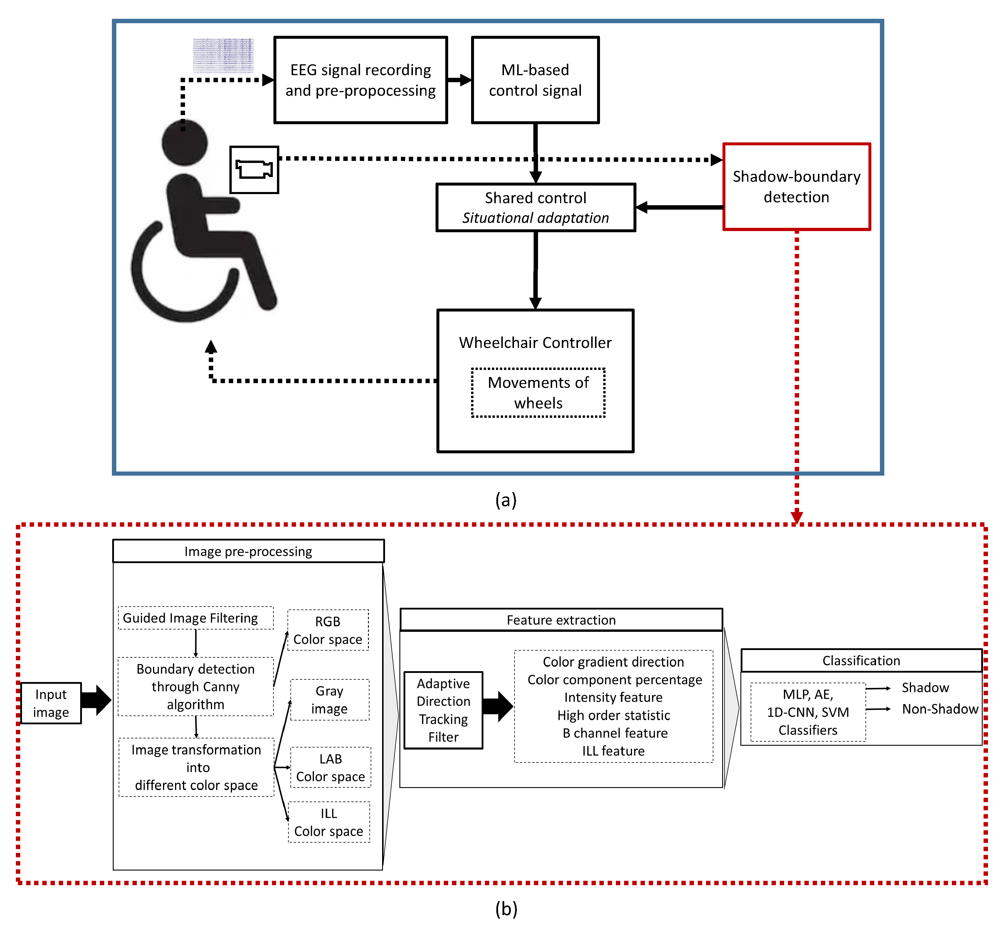
3. Proposed BMI System

The overall block diagram of the proposed BMI prototype for controlling wheelchairs is illustrated in Figure 1a. EEG signal recording and pre-processing. EEG signals are recorded by means of a set of 19 electrodes (Fp1, Fp2, F3, F4, C3, C4, P3, P4, O1, O2, F7, F8, T3, T4, T5, T6, Fz, Cz, and Pz) placed according to the 10–20 International System. Each signal is band-pass filtered at 0.5–40 Hz, in order to process the main EEG sub-bands: $\delta$ (0.5–4 Hz), $\theta$ (4–8 Hz), $\alpha$ (8–12 Hz), $\beta$ (12–32 Hz) and $\gamma$ (32–40 Hz). The subject sits comfortably on a chair and is instructed to perform mental tasks according to the paradigm proposed in [40]. Notably, four tasks are planned: Task 1 (baseline measurement), the subject is relaxed without performing/imaging any task; Task 2 (forward) the subject is asked to look at an upward arrow shown on a monitor and imagine (for 10 s) to move both hands towards the same arrow direction (i.e., forward); Task 3 (left), the subject is asked to look at a left arrow shown on a monitor and imagine (for 10 s) to move the left hand towards the same arrow direction (i.e., left); finally, Task 4 (right), the subject is asked to look at a right arrow shown on a monitor and imagine (for 10 s) to move the right hand towards the same arrow direction (i.e., right). ML-based control signal. BMI is based on the capability to discriminate different brain activity patterns, each being related to a specific mental task. Hence, the control signal plays a key role in the proposed BMI system. Specifically, subjects need to modulate their own cerebral waveforms in order to produce accurate and appropriate brain patterns. To this end, ML algorithms are employed to extract significant EEG-features and automatically classify the mental tasks (i.e, relax, foward, right, left) performed by the user.

Wheelchair controller. The decoded EEG recordings (i.e., EEG-features) are mapped into directional control commands to drive the wheelchair [41]. Specifically, turn left, turn right, go forward and rest. Contextually, a shadow detection system is proposed to identify boundary areas along to the direction of the wheelchair and alert the user from potential obstacles. Shadow detection system. A camera is installed on the wheelchair to capture the surrounding scene and the proposed boundary detection algorithm is performed (Figure 1b). Shared control. The output of the proposed shadow-boundary detection algorithm is fused together with the control signal (produced by the metal task), resulting in a multi-modal BMI strategy. Such shared control logic is able to self-adapt to the situation. Note that there is a time delay between the motor imagery and decoding of a specific movement into the corresponding directional command able to move the wheelchairs. The shared control operates in this time frame. For example, when the shadow detection system recognizes a potential obstacle, overwrites the mental control and activates a security procedure by stopping or changing the direction of wheels. Note that, in study, the development of the shadow detection module is addressed and widely detailed in the subsequent sections.

3.1. Dataset Description

In this study, images gathered from LabelMe [42] are used. LabelMe dataset created by MIT Computer Science and Artificial Intelligence Laboratory (CSAIL) includes (to date) 187,240 images, 62197 annotated images and 658992 labeled objects. Furthermore, several casual street scenes from MIT CSAIL Database [43] captured by customers are also included in LabelMe. Here, due to the limited computational power available (laptop with a 3.1 GHz Intel Core i5 processor, 8 GB memory), 100 images are selected randomly.

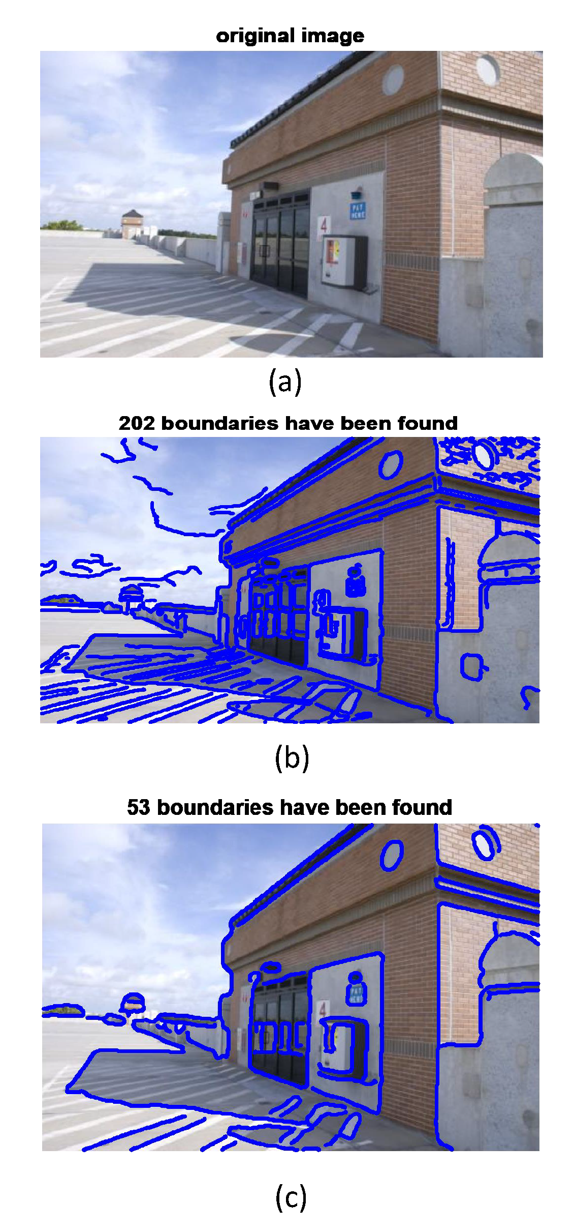
3.2. Image Pre-Processing

The original RGB image is sharpened to overcome blurring effect (introduced by cameras) and emphasize edge contrast to increase legibility. Using guided-filter [44], users can strengthen the edges and reduce the noise from image. The boundaries of objects are then selected with the canny edge detection method [45]. The threshold parameter and standard deviation in canny edge detection are also calibrated to find an optimal result able to further reduce the feature extraction. As an example, canny detection is applied after guided-filter to the original image shown in Figure 2a. It is worth mentioning that, using the default values of parameters results in 202 boundaries (Figure 2b), while setting the two threshold parameters to 0.08, 0.2 and standard deviation $\sigma$ = 3 leads to a reduced number of shadow boundaries (Figure 2c). Hence, in this study, we use this optimized set of parameters. Finally, the RGB image is converted into three color spaces: Gray, LAB and ILL for further investigating the features of shadow [46].

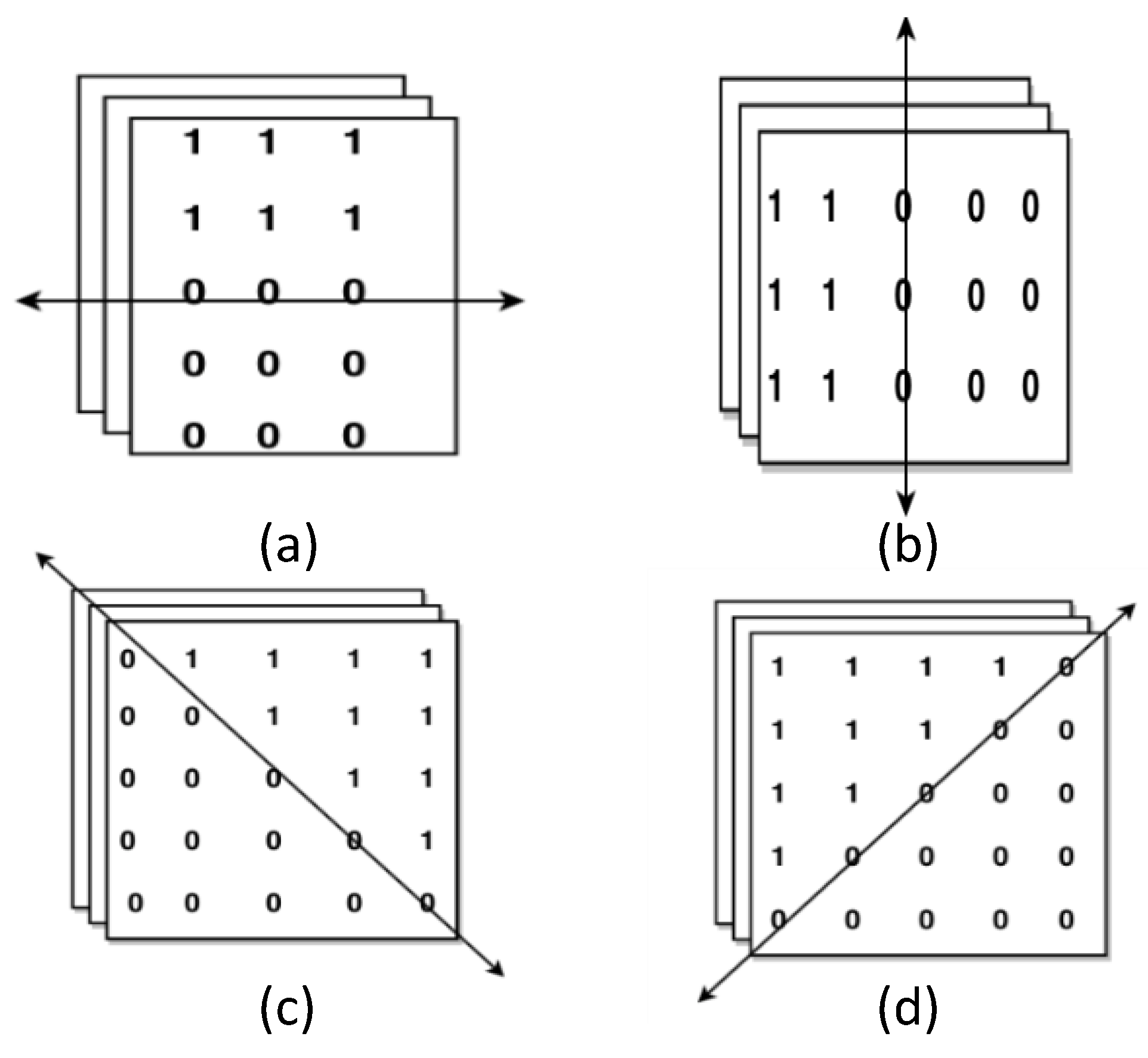
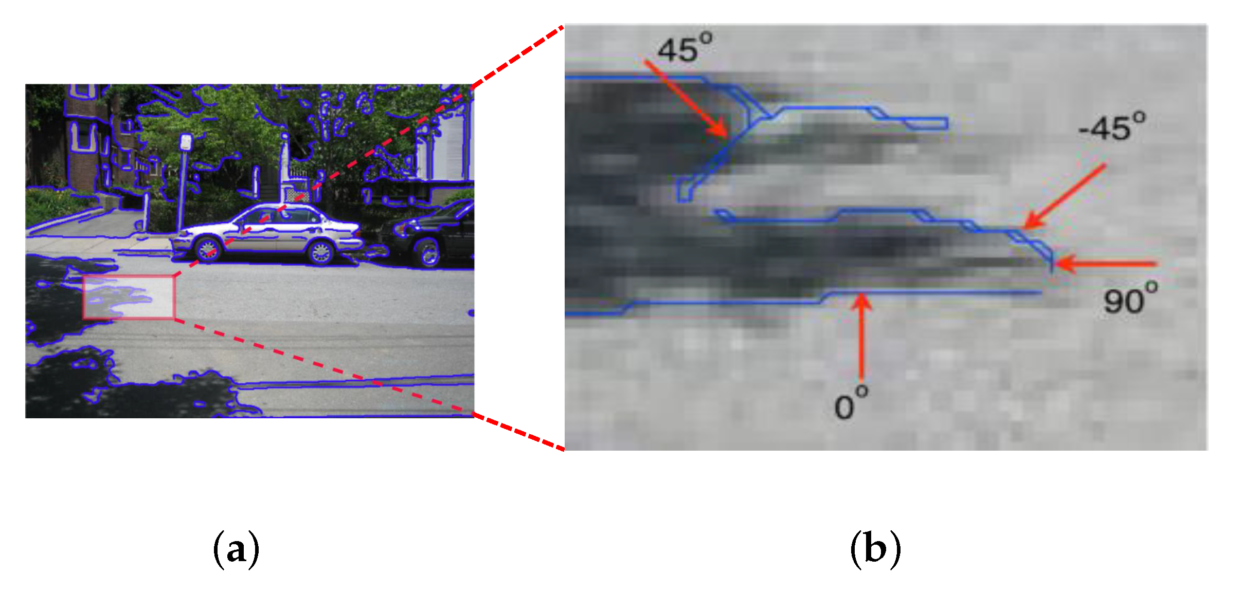
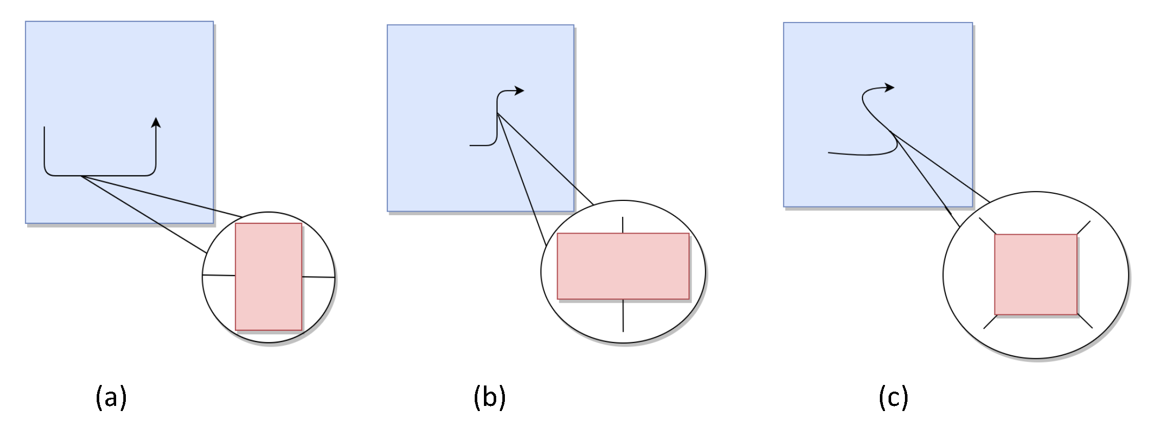
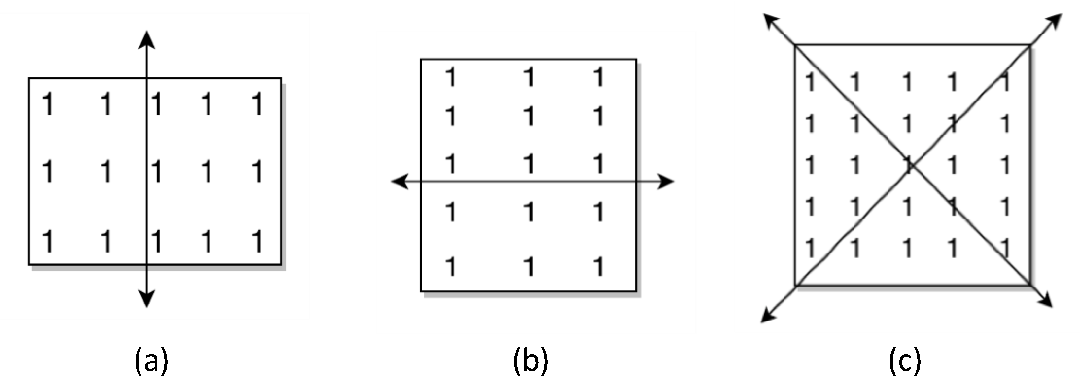
3.3. Design of Adaptive Direction Tracking (ADT) Filter

The aim of the proposed adaptive direction tracking (ADT) filter is to extract features along the boundary direction. Shadow boundaries can be extended to almost every possible direction as shown in Figure 3a. However, four directions can be set in the modelling method: $0^{\circ }$ in horizontal direction, ${90}^{\circ }$ in vertical direction, ${45}^{\circ }$ and −${45}^{\circ }$ in diagonal directions as shown in Figure 3b. The direction of boundaries can be calculated through coordinates of adjacent pixels using canny edge detection algorithm. The shape of ADT filter depends on its function and can be customized by users. In this work, the shape of the filter is designed as shown in Figure 4.

The ADT filter is developed into a rectangle or a square shape, in accordance with the following rules. The rectangle ADT filters applied on images are sized $\tau$ × 3 or 3 × $\tau$, where $\tau$ represents the length of the filter, while square filters are sized $\tau$ × $\tau$. Furthermore, the ADT filter is designed as shown in Figure 5. Features are evaluated on both sides of each boundary. It is to be noted that each layer of ADT filter shares the same weight coefficients. When the ADT filter moves along the boundary, the information of the extracted feature will be automatically collected from one side of the boundary through the positive parts with values of 1, such as the upper part of filter in Figure 5a. The same operation is performed to collect information on the other side of the boundary by rotating the filter by 180^∘.

3.4. Feature Extraction

In this study, given a pixel under analysis, the ADT filter is employed to extract the following features: color gradient direction, color component percentage, intensity, high order statistic, B channel and Illumination Invariant (ILL) feature.

Color gradient direction feature. According with Huang et al. [9], the reflectance of a shadow boundary for each pixel is locally constant, hence, the color gradient direction is identical in each channel, since the RGB illumination gradients are all perpendicular to shadow boundary. After calculating three gradient directions by Sobel filter, the gradient direction difference is measured for each color as follows:

$${\rho }_{rg}=min(|{\rho }_r-{\rho }_g|,2\pi -|{\rho }_r-{\rho }_g|)$$

(1)

$${\rho }_{gb}=min(|{\rho }_g-{\rho }_b|,2\pi -|{\rho }_g-{\rho }_b|)$$

(2)

$${\rho }_{br}=min(|{\rho }_b-{\rho }_r|,2\pi -|{\rho }_b-{\rho }_r|)$$

(3)

where ${\rho }_r$ is the gradient direction of red channel, ${\rho }_g$ and ${\rho }_b$ represent the gradient direction of green channel and blue channel, respectively, while 2$\pi$ is used to achieve the translation of the absolute value of the gradient direction difference under analysis. Hence, a color gradient direction feature vector sized 1 × 3 is extracted.

Color component percentage feature. The component percentage feature, especially the blue component ratio in RGB color space is very important in detecting shadow boundaries [9]. Shadow has a blue mask under the sun, consequently, the proportion of blue chromatic content takes more percentage in RGB color space. However, it is worth mentioning that it is impossible to distinguish shadow boundaries from other object boundaries by only such feature, because some object boundaries may share the similar properties. Hence, ratio of blue component to other color components is used to avoid error from detecting boundaries and consequently improve the accuracy significantly. Since the pixel values in shadow are always lower than those in sunlit areas, high values represent bright areas while low values represent shadow areas. Let define the following ratios:

$$T_r=(L_r+1)/(H_r+1)$$

(4)

$$T_g=(L_g+1)/(H_g+1)$$

(5)

$$T_b=(L_b+1)/(H_b+1)$$

(6)

where $H_r$, $H_g$, $H_b$ are pixel values of bright, sunlit edge for red green and blue channels, respectively; while, $L_r$, $L_g$, $L_b$ are those for the dark edge. In order to enhance accuracy performance in determining shade, we defined $T_{all}$, $T_{br}$ and $T_{bg}$ to represent the ratio of blue component at each pixel in RGB color space, where:

$$T_{all}=T_b/(T_r+T_g+T_b))$$

(7)

$$T_{br}=T_b/T_r$$

(8)

$$T_{bg}=T_b/T_g$$

(9)

Hence, a color component percentage feature vector sized 1 × 3 is extracted.

Intensity feature. Such feature is typically used in several shadow detection algorithms for its discriminative properties [11,47,48]. The original image is transformed into a gray scale image to obtain the intensity of illumination on object boundaries. Such feature is evaluated on both side of the boundary by applying 3 ADT filters sized 5 × 3, 7 × 3 and 11 × 3, respectively. The result is an intensity features vector of 1 × 6 (as 3 values per side are estimated). It is to be noted that if the light intensity feature on both sides of a pixel are the same, the pixel under analysis does not belong to the shadow edge.

High Order Statistic (HOS) features. Here, HOS analysis includes the extraction of two features: skewness $\gamma$ and kurtosis $\kappa$. Skewness is a measure of the asymmetry of the probability distribution for a real-valued random variable defined as:

$$\gamma =E\left[{\left(\frac{(X-\mu )}{\sigma }\right)}^3\right]$$

(10)

where $\mu$ is the mean value, $\sigma$ is the standard deviation, E is the expectation operator. The skewness of data is calculated on the direction of object boundaries. Kurtosis $\kappa$ defined as follow:

$$\kappa =E\left[{\left(\frac{(X-\mu )}{\sigma }\right)}^4\right]$$

(11)

where $\mu$ is the mean value, $\sigma$ is the standard deviation, E is the expectation operator. Figure 6 shows the filter structure for collecting HOS features in different directions. Similarly to the intensity feature, 3 filters are applied to each side of the boundary. The only difference from ADT filter is that now all the coefficients are 1. Hence, a HOS feature vector sized 1 × 6 is extracted.

B channel feature. B channel represents the blue–yellow component, extracted from the LAB color space. It has been proved to be a suitable information to distinguish the shadow from image [29]. Instead, it is to be noted that A channel is invariant to shadows [49]. Direct sunlit area appears yellow, while the rest area reflected by the sky appears blue [50,51]. This means that the content of shadow boundary will transit from blue to yellow in LAB’s B channel. We applied ADT filters as for the intensity feature, extracting a B channel feature vector sized 1 × 6.

Illumination Invariant (ILL) feature. The last feature illumination invariant (ILL) is estimated from all three channels using the perception-based color space [46]. For each channel two different ADT filters (sized 5 × 3, 7 × 3, respectively) are applied to both sides of the boundaries, producing 4 values. As results 4 × 3 (number of channels) = 12 features are evaluated.

Overall, a 36-dimensional feature vector is estimated and used input the proposed machine learning classifiers.

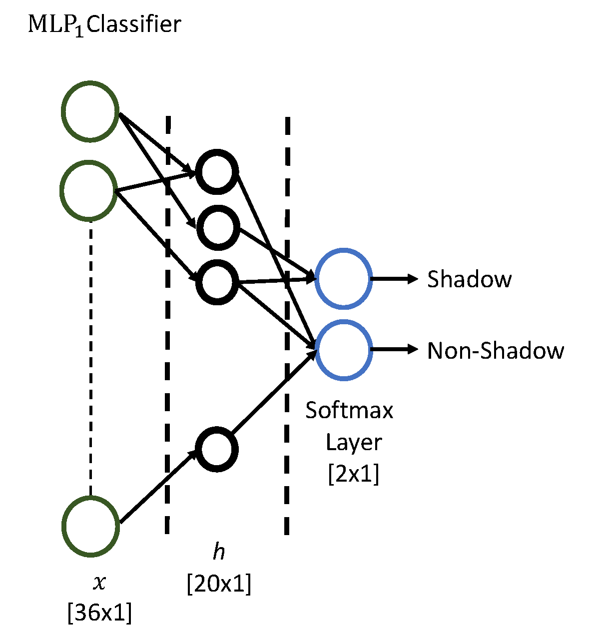
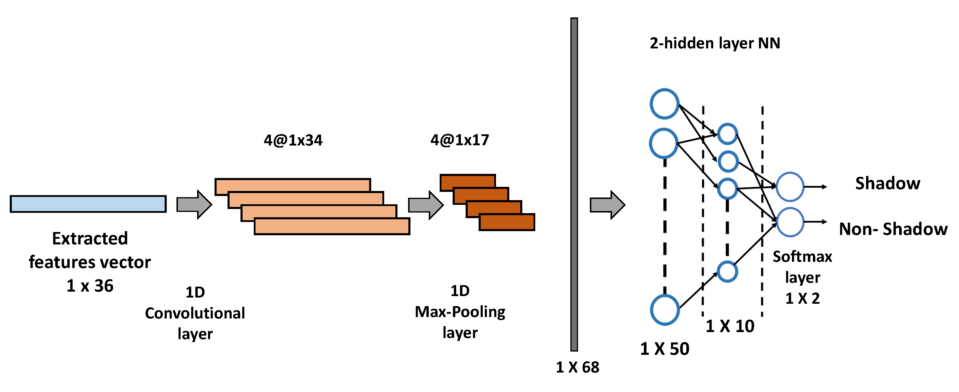
3.5. Machine Learning Models

The extracted features are used as input to four machine learning based classifiers: Multilayer Perceptron (MLP), Auto-encoder (AE), 1D-Convolutional Neural Network (1D-CNN), Support Vector Machine (SVM).

MLP classifier: MLP is the most common feed-forward neural network, that uses standard gradient backpropagation method [52] to minimize the difference between the estimated and target values. It typically consists of one input layer, one output layer and one or more hidden layers [53]. Here, three MLP models are developed: MLP₁ composed of 1 hidden layer with 20 hidden neurons; MLP₂ composed of 1 hidden layer with 10 units; MLP₃ composed of 2 hidden layers with 20 and 10 neurons, respectively. All the developed networks are trained for about 10³ epochs on a laptop with a 3.1 GHz Intel Core i5 processor with 8GB memory installed. Note that the saturating linear transfer function is used as activation (since it provided good classification results) and that all MLP models end with a softmax output layer for performing the binary classification task (shadow vs. non-shadow). As an example, Figure 7 shows the MLP₁ architecture.

AE classifier: AE model is trained through unsupervised learning algorithm and aims at generating the original data from the compressed representation of the input by an encoder-decoder operation [54]. Notably, the encoder compresses the input pattern (x) into a lower dimensional space (h):

$$h=f(xW+b)$$

(12)

where W is the weight matrix, b the bias vector and f the activation transfer function for the encoder. The decoder attempts to reproduce the original data from the compressed representation:

$$\overline{x}=\overline{f}(h{\overline{W}}^T+\overline{b})$$

(13)

where $\overline{f}$, $\overline{W}$, $\overline{b}$ are the corresponding activation function, weight matrix, bias in the decoder module. In this study, for fair comparison, three AE, denoted as AE₁, AE₂, AE₃ with similar topology of MLP₁, MLP₂, MLP₃, respectively are developed. For example, AE₁ (whose architecture is 36:20:36, Figure 8a) extracts 20 features (from the 36-dimensional input vector) used as input to softmax layer (trained in supervised modality) to perform the 2-way classification. Next, fine-tuning technique is applied by training again the whole network depicted in Figure 8b and sized 36:20:2. Similarly, AE₂ and AE₃ were developed. Note that all AE classifiers used saturating linear transfer activation function and were trained for about 10³ epochs.

1D-CNN classifier: CNN is a deep learning architecture typically used in 2D-image classification or pattern recognition [55,56,57,58,59,60]. However, 1D-CNN is also employed to process 1D-patterns for discrimination purposes [61]. A common CNN includes different processing layers of convolution, activation, pooling, followed by a feed-forward MLP with softmax output layer. Notably, the first layer is composed of a set of S filters that computes the dot product with a local input region selected by the filter. Every filter moves with a step size s, performing the convolution operation. S features maps are produced. The second layer is typically a rectified linear unit (ReLU) f(x) = max (x,0), employed for its effectiveness, simplicity and also because it provides non upper-bounded output values. The third layer performs the pooling operation. In particular, a filter moves along the input features maps (extracted by the previous layer) and estimates the maximum or average value. The output is a downsampled representation od the input data. It is to be noted that, here, the max pooling operation is used for its good translational-invariant properties [62]. Finally, a fully connected MLP performs the discrimination task. Further details are reported in [63]. In this study, the proposed 1D-CNN is composed of 1 convolutional layer (followed by a ReLU activation function), 1 max pooling layer and MLP for classification purposes (Figure 9). Specifically, the proposed CNN is modelled to receive as input the extracted features vector sized 1 × 36. The convolutional layer is composed of 4 1-dimensional filters sized 1 × 3, stride s = 1 and padding p = 0, resulting in 4 features vectors sized 1 × 34. After applying the ReLU transfer function, the max-pooling, composed of a filter sized 1 × 2 and step size 2, reduces the input spatial resolution from 1 × 34 to 1 × 17. Next, the 4 features vectors are reshaped into a single 1-dimensional vector of dimension 1 × 68 and fed into a 2-hidden layers neural network (with 50 and 10 hidden units, respectively) followed by a softmax output layer for the 2-way pixel-based classification task: shadow vs. non-shadow. The proposed 1D-CNN was trained with stochastic gradient descent optimizer with learning rate of 0.1 for about 10³ iterations until the cross-entropy function converged. It is to be noted that the topology of the proposed 1D-CNN was set-up by using a trial-and-error approach. Here, we reported the configuration that showed the best results.

SVM classifier: SVM is a statistical technique that finds the best hyperplane able to provide the maximum separation among classes. Here, the radial basis function (RBF) kernel is used to develop the SVM classifier and perform the shadow detection task. Further details of SVM are reported in [64].

4. Results and Discussion

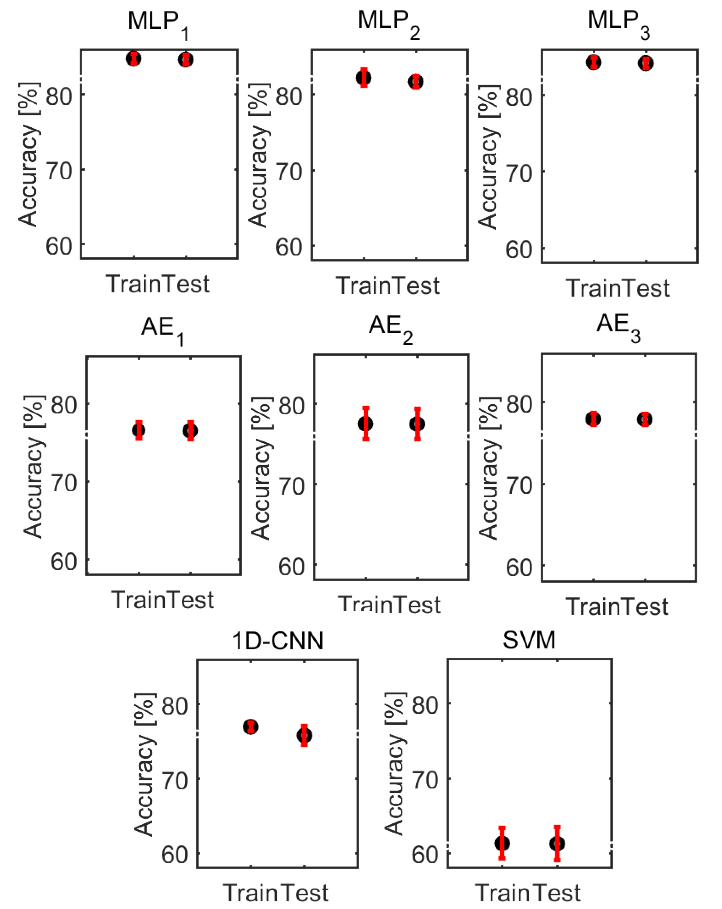
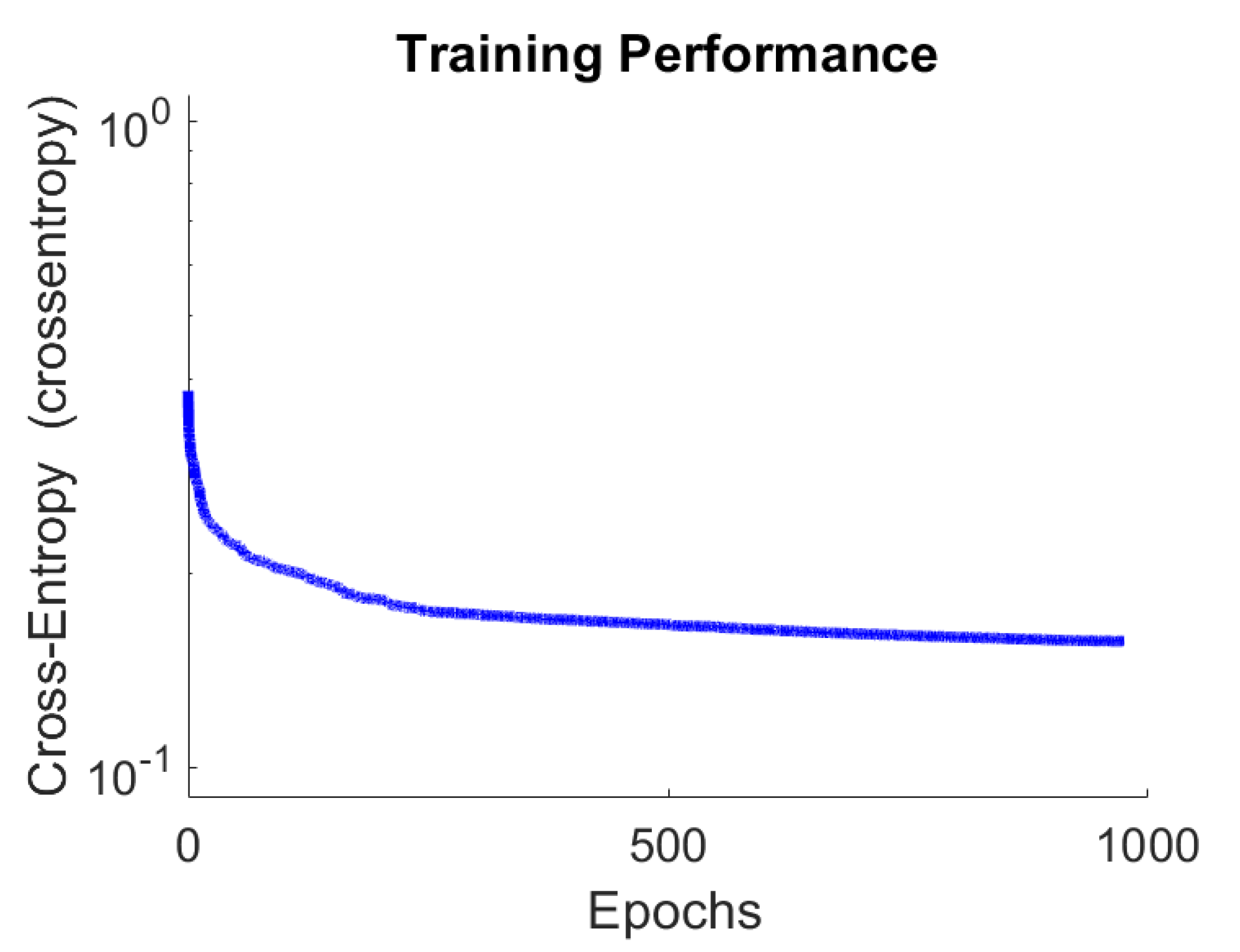
4.1. Performance of the Proposed System

The dataset used in the present study included 100 images with shaded areas gathered from LabelMe [42]. Given an image under analysis, boundary pixels were selected through Canny method [45] and for each pixel 36 features were evaluated through the proposed ADT filter (Section 3). An overall of 389856 36-dimensional feature vectors were taken into account (194928 belonging to the shadow pixel class and 194928 to the non-shadow pixel class) and used as input to the developed MLP, AE, 1D-CNN, SVM classifiers to perform the 2-way pixel-based classification task: shadow vs. non-shadow. Standard metrics (i.e., Accuracy (A), Recall (R), Precision (P), F-measure (FM)) were employed to assess the effectiveness of the proposed classifiers:

$$A=\frac{TP+TN}{(TP+FP+TN+FN)}$$

(14)

$$R=\frac{TP}{(TP+FN)}$$

(15)

$$P=\frac{TP}{(TP+FP)}$$

(16)

$$FM=2\times \frac{P\times R}{(P+R)}$$

(17)

where TP, FP, TN, FN represent the true positive, false positive, true negative and false negative, respectively. Furthermore, the k-fold cross validation (with k = 7) procedure was also applied for quantifying the discrimination performance. In particular, for each class, train set consisted of 70% of instances and test set of remaining 30%. Hence, all evaluation performance are reported as average value ± standard deviation. It is worth noting that the proposed MLP/SVM/CNN are supervised learning approaches and use the class label information in the training procedure. In contrast, AE is trained with unsupervised learning, hence the label was not used during the training phase. The extracted features from unlabeled data were the input to a softmax layer for classification purposes. The whole network is then fine-tuned to enhance performance.

Table 1. Comparative results of the proposed MLP, AE, 1D-CNN, SVM classifiers evaluated on the test sets. All the outcomes are reported as mean value ± standard deviation.

Model	Precision	Recall	F-Measure	Accuracy
MLP1	82.72 ± 0.77%	87.52 ± 0.4%	85.05 ± 0.57%	84.63 ± 0.63%
MLP2	79.47 ± 0.97%	85.55 ± 0.66%	82.39 ± 0.69%	81.71 ± 0.77%
MLP3	82.6 ± 0.66%	86.6 ± 0.45%	84.55 ± 0.53%	84.19 ± 0.56%
AE1	74.27 ± 0.99%	81.14 ± 1.47%	77.55 ± 1.03%	76.51 ± 1.04%
AE2	75.5 ± 1.99%	81.44 ± 1.42%	78.36 ± 1.71%	77.51 ± 1.89%
AE3	75.67 ± 0.77%	82.29 ± 0.75%	78.84 ± 0.66%	77.91 ± 0.72%
1D-CNN	73.5 ± 1.91%	81.0 ± 2.3%	76.90 ± 1%	75.80 ± 1.2%
SVM	62.5 ± 3.88%	58.6 ± 9.64%	59.93 ± 3.85%	61.27 ± 2.18%

reports the pixel detection performance (evaluated on test sets) in terms of averaged precision, recall, F-measure, accuracy for the MLP, AE, 1D-CNN and SVM classifier. In relation to MLP classifiers, MLP₁ outperformed MLP₂ and MLP₃, achieving F-measure and accuracy values of 85.05 ± 0.57% and 84.63 ± 0.63% respectively. However, it is to be noted that high performance were observed also with MLP₂ (F-measure of 82.39 ± 0.69%, accuracy of 81.71 ± 0.77%) and MLP₃ (F-measure of 84.55 ± 0.53%, accuracy of 84.19 ± 0.56%). In relation to AE classifiers, the model with two hidden layer denoted as AE₃, produced F-measure and accuracy rates up to 78.84 ± 0.66% and 77.91 ± 0.72%, respectively. Very good results were achieved also by AE₁ and AE₂. In particular, the average accuracies were of 76.51 ± 1.04% and 77.51 ± 1.89%, respectively. As regards the proposed 1D-CNN (Figure 9) the following average perfomance were achieved: accuracy of 75.8 ± 1.2%, precision of 73.5 ± 1.91%, recall of 81.0 ± 2.3% and F-measure of 76.9 ± 1%. Finally, as regards SVM classifier, lower average performance were achieved: precision of 62.5 ± 3.88%, recall of 58.6 ± 9.64%, F-measure 59.93 ± 3.85%, accuracy of 61.27 ± 2.18%. Hence, comparative simulation results showed that the proposed MLP₁ classifier achieved the highest pixel-based detection performance (accuracy of 84.63 ± 0.63%) as compared to MLP₂, MLP₃, AE₁, AE₂, AE₃, SVM classifiers. In support of this result, the Area Under the Curve (AUC) of the Receiver Operating Characteristic (ROC) was estimated. Specifically, Figure 10 shows the average values of AUC and related ROC curves, evaluated for the developed MLP, AE, 1D-CNN, SVM classifiers. As can be seen, MLP₁ outperformed all the other approaches reporting an AUC = 92 ± 0.53%. It is worth noting that, overtraining and overfitting issues were also studied to assess the effectiveness of the developed models. Specifically, in order to control the aforementioned phenomenon, the k-fold cross validation (k = 7) technique was adopted and train accuracies were also compared with those achieved in the test phase. Note that the following data separation was employed: 70% for train and 30% for test. As can be seen from Figure 11, all the proposed models were not deficient of overtraining or overfitting and provided good generalization abilities, reporting a small standard deviation and a maximum gap between train and test average accuracy of only 1%. Furthermore, networks were trained until the converge of the cross-entropy function was observed. As an example, Figure 12, reports the training phase of the best classifier proposed in this study, i.e., MLP₁. However, it is also worth mentioning that the topology of the classifiers, learning and training parameters were set-up performing several experimental tests according to a trial and error approach.

Hence, experimental results showed that the proposed MLP₁ classifier achieved the best detection performance when compared with other machine learning techniques (i.e., MLP₂, MLP₃, AE₁, AE₂, AE₃, 1D-CNN, SVM) as well as other previous shadow detection approaches [9,11], reporting accuracy and AUC rates up to 84.63 ± 0.63% and 89 ± 0.8%, respectively. It is interesting to note that MLP outperforms AE and 1D-CNN classifiers (that belongs to more advanced machine learning architectures [65]). This is possible due to the limited size of input space (only 36 features). Indeed, DL-based approaches are typically used to big data with a large input dimension. Here, the proposed AE may cause an over compression of features and hence a loss of significant information; while the hierarchical learning representation of a standard CNN is too complex to cope with the pixel-based classification task of this study. For these reasons, common machine learning algorithms with a simpler architecture (i.e., MLP) achieved better results. It is worth noting that also the developed AE and 1D-CNN achieved very good results. In particular, AE₃ reported detection accuracy of 77.91 ± 0.72%, whereas 1D-CNN reported accuracy of 75.8 ± 1.2%.

4.2. Permutation Analysis

The effectiveness of the developed classifiers was measured using the k-fold cross validation technique, reporting average accuracy rate up to 84.63 ± 0.63%. However, in order to prove that the estimated classification results are not achieved by chance, the permutation-based p-value statistical test is performed [66]. Permutation analysis consists in evaluating the p-value under a specific null hypothesis, that is: features and targets are independent. To this end, M permutations of the labels are generated and the corresponding statistical measure (here, the accuracy) is evaluated. Overall, A_j accuracy values are estimated (with j = 1, 2, …, M). Then, the p-value is calculated as fraction between the number of A_j accuracies equal or higher than the accuracy rate evaluated with the original features-labels relationship (i.e., 84.63%) and the total number of permutations (i.e., M). If p-value is smaller than a certain threshold $\alpha$ (generally 0.05), the null hypothesis is rejected leading to the conclusion that the classifier is statistically independent. Ideally, all the possible permutations of the labels should be tested; but, since this is computationally too much expensive, M = 100 is used (as it has been shown to produce stable results [66]). Simulation results reported that p-value = 0.00/100 = 0.00 < 0.05. Hence, the null hypothesis was rejected and the developed classifier is statistically significant.

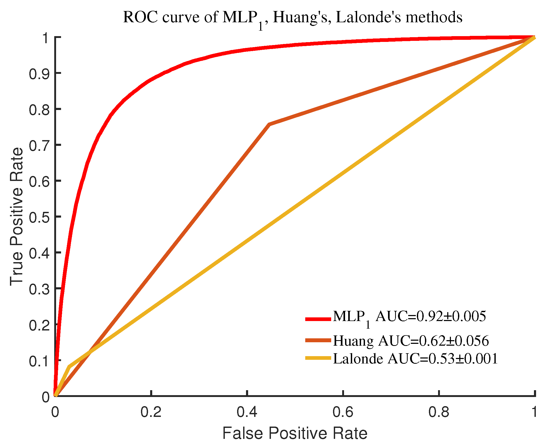
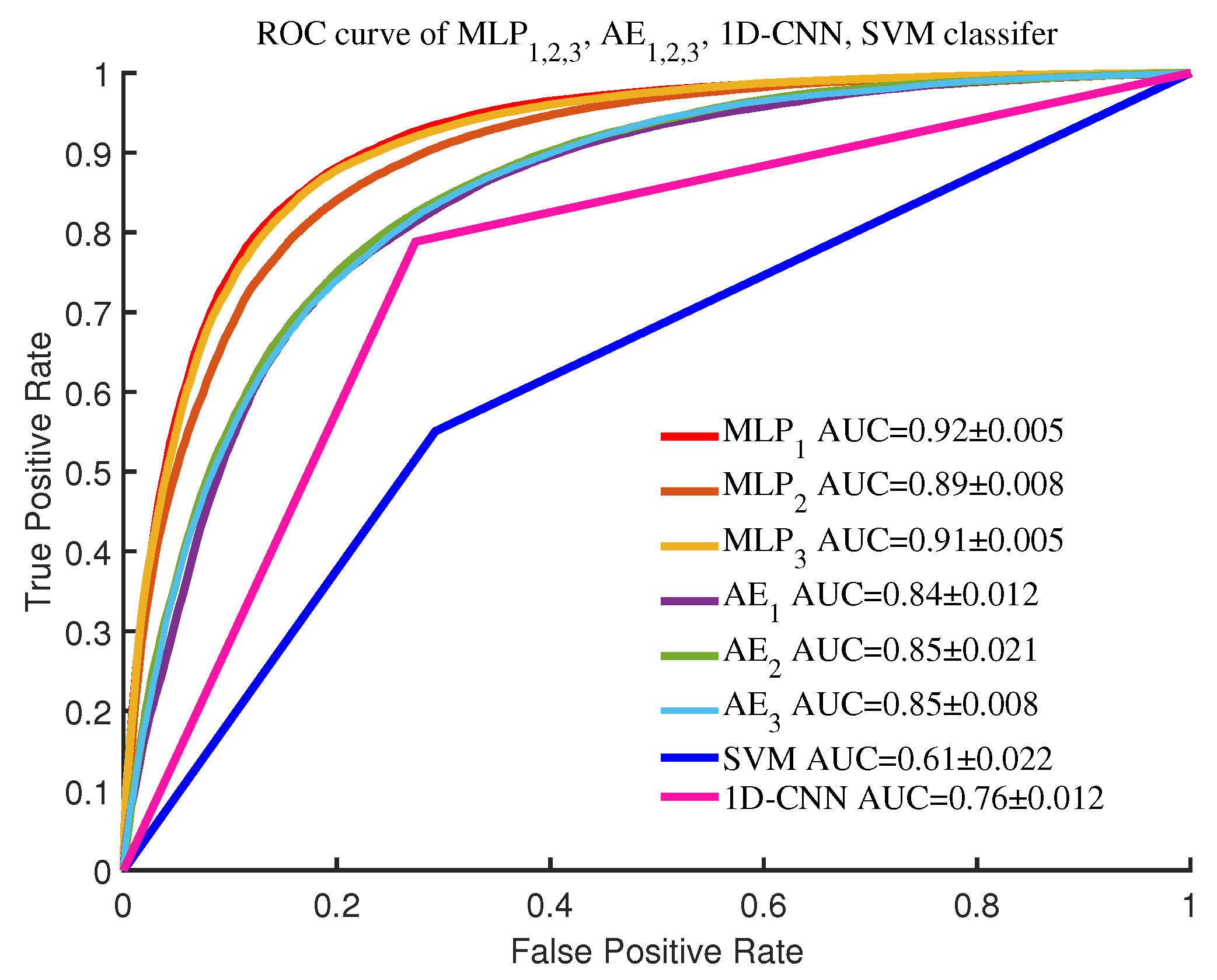
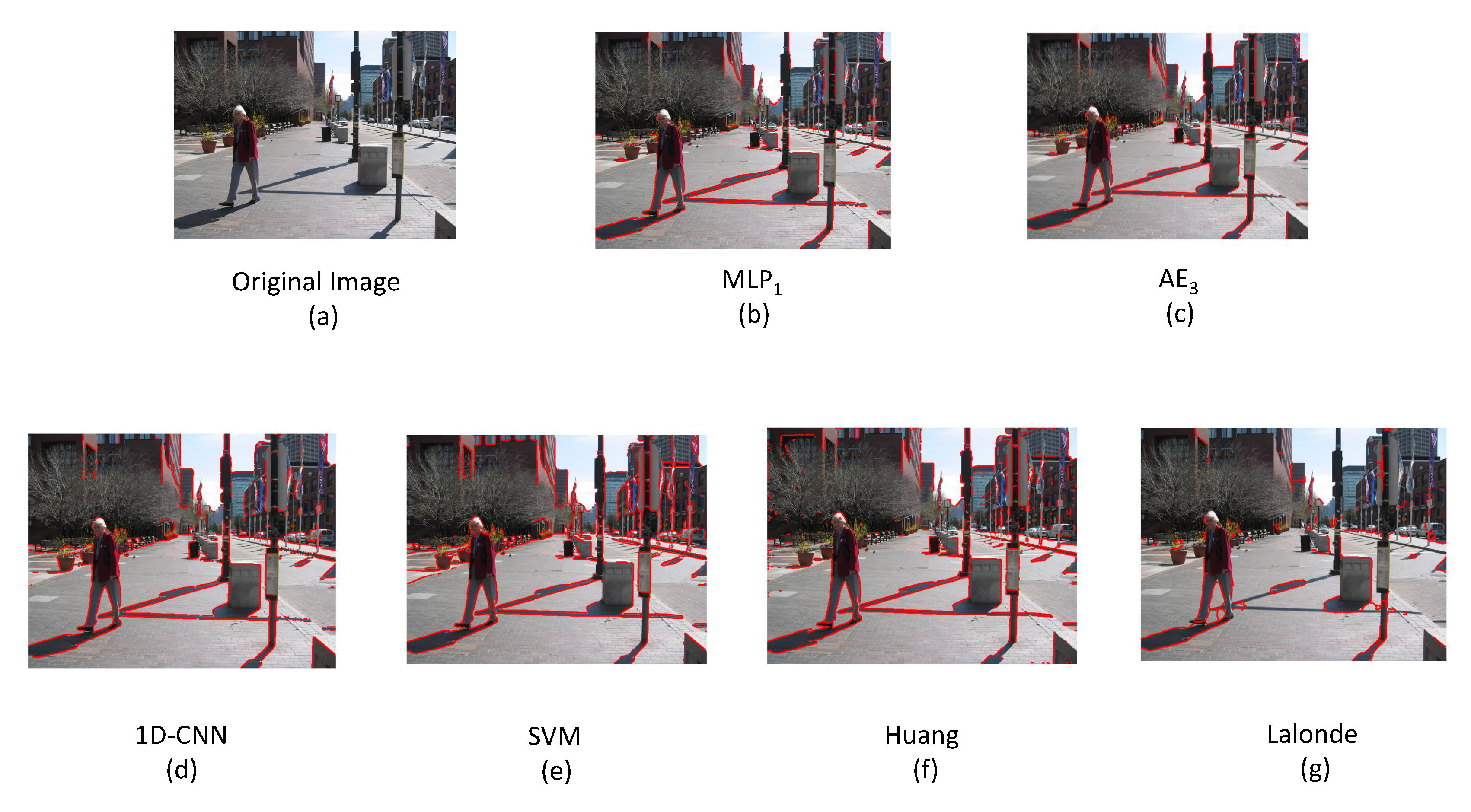
4.3. Comparison of Shadow Detection Models

The proposed ADT filter based machine learning shadow boundary detection system was also compared with other approaches reported in the literature. In particular, here Huang’s [9] and Lalonde’s [11] approaches were taken into account. In [9] Huang et al. proposed a physical model of shadow able to compute the width, shape, color of the penumbra and extract some visual features such as shadow sharpness, dark to bright slope, dark to bright ratio and dark to bright gradient used as input to a RBF-based SVM classifier to perform shadow detection task. In [11] Lalonde et al. proposed a decision tree classifier for pixel shadow detection. Specifically, they used a CRF-based optimization to concatenate the shadow pixels to produce a more coherent shadow contour and remove the high unlikely shadow boundaries and isolate weak edges. In contrast, in this study, we propose an ADT filter able to extract HOS and optical features only along the direction of boundary (in simple and complex real scenes) avoiding redundant information [67]. The estimated parameters are then used as input to a very simple and computationally not expensive MLP architecture to perform the 2-way classification task: shadow vs. non-shadow. Furthermore, since Huang’s and Lalonde’s approaches are fully publicly available, for fair comparison we decided also to apply such methods on the same images dataset used in the present study. Comparative experimental results are reported in

Table 2. Comparative results of our proposed shadow detection system (i.e., MLP₁), Huang’s and Lalonde’s methods evaluated on the test sets. All the outcomes are reported as mean value ± standard deviation.

Model	Precision	Recall	F-Measure	Accuracy
MLP1	82.72 ± 0.77%	87.52 ± 0.4%	85.05 ± 0.57%	84.63 ± 0.63%
Huang	60 ± 4.91%	77.17 ± 5.50%	67.37 ± 4.10%	62.52 ± 5.54%
Lalonde	74.03 ± 0.75%	8.19 ± 0.12%	14.74 ± 0.21%	52.67 ± 0.1%

. As can be seen, accuracies of 84.63 ± 0.63%, 62.52 ± 5.54% and 52.67 ± 0.1% were achieved by our proposed detection system (i.e. MLP₁), Huang’s and Lalonde’s approaches, respectively. Hence, our proposed MLP₁ classifier reported the highest performance. Similar result was observed also by evaluating the AUC as reported in Figure 13. As an example, Figure 14 shows the shadow detection results achieved by MLP, AE, 1D-CNN, SVM, Huang’s and Lalonde’s approaches of a realistic scene. Note that only the best MLP and AE classifiers are reported (i.e., MLP₁, AE₃). As can be seen MLP₁ is able to detect shadow boundaries better than other approaches; indeed, 1D-CNN, SVM and Huang’s classifiers detect also buildings and other profiles of the scene that do not belong to a shadow, whereas Lalonde’s is deficient to identify shaded areas. Finally, as previously mentioned, AE₃ shows considerable discrimination capability. However, the proposed shadow detection system (i.e., MLP₁) has some drawbacks. Features of object boundaries may be similar to those features of shadow boundaries, causing a misclassification of the pixel under analysis. Furthermore, the extracted features are based on physical characteristics, hence, when the intensity of light is weak or when the shadows lie on some special material surface that can cause a significant change of physical properties, the shaded boundary is very difficult to identify. Last limitation is that our proposed system (i.e., MLP₁) may include also the object profile in the detection process, as shown in Figure 14b.

5. Summary and Future Works

In this paper, we proposed a BMI prototype for controlling wheelchairs by using decoded EEG signals recorded while the user performs tasks to drive the wheels. The novelty of the proposed system lies in including a shadow detection module based on an adaptive direction tracking filter to extract target features along the direction of boundaries. Note that the present study is intended as preliminary work for a future full BMI system implementation. Here, we propose a theoretical framework for controlling the navigation of a wheelchair. At this stage, BMI experiments and validation have been conducted through a laboratory set-up. A novel shadow detection strategy is developed based on an adaptive direction tracking filter for use in the BMI wheelchair system. Note that the integration of the proposed detection algorithm with the BMI, including real-time wheelchair control testing, is proposed as future work. Future development can also focus on motor imaginary experiments, EEG recordings, classification of the control signal using ML-techniques, acquisition of real scenes from a camera installed on the wheelchair and a detailed shared control strategy that adapts to the situation and alarms the user of possible obstacles. In addition, motivated by the promising shadow detection results achieved, in this study, our follow-up work will consider a wider set of features (such as those reported in [12,68]). Moreover, optimization techniques [69] for tuning the training parameters and deep learning approaches [70,71,72] will be explored in an attempt to enrich the shadow detection accuracy.

References

1. Carmena, J.M.; Lebedev, M.A.; Crist, R.E.; O’Doherty, J.E.; Santucci, D.M.; Dimitrov, D.F.; Patil, P.G.; Henriquez, C.S.; Nicolelis, M.A. Learning to control a brain–machine interface for reaching and grasping by primates. PLoS Biol. 2003, 1, e42. [Google Scholar] [CrossRef] [PubMed] [Green Version]
2. Solé-Casals, J.; Caiafa, C.F.; Zhao, Q.; Cichocki, A. Brain-Computer Interface with Corrupted EEG Data: A Tensor Completion Approach. Cogn. Comput. 2018, 10, 1062–1074. [Google Scholar] [CrossRef] [Green Version]
3. Ullman, S. High-Level Vision: Object Recognition and Visual Cognition; MIT Press: Cambridge, MA, USA, 1996; Volume 2. [Google Scholar]
4. Russell, M.; Zou, J.J.; Fang, G. An evaluation of moving shadow detection techniques. Comput. Vis. Media 2016, 2, 195–217. [Google Scholar] [CrossRef] [Green Version]
5. Xiang, J.; Fan, H.; Liao, H.; Xu, J.; Sun, W.; Yu, S. Moving object detection and shadow removing under changing illumination condition. Math. Probl. Eng. 2014, 2014, 827461. [Google Scholar] [CrossRef] [Green Version]
6. Liasis, G.; Stavrou, S. Satellite images analysis for shadow detection and building height estimation. ISPRS J. Photogramm. Remote Sens. 2016, 119, 437–450. [Google Scholar] [CrossRef]
7. Okabe, T.; Sato, I.; Sato, Y. Attached shadow coding: Estimating surface normals from shadows under unknown reflectance and lighting conditions. In Proceedings of the 2009 IEEE 12th International Conference on Computer Vision, Kyoto, Japan, 29 September–2 October 2009; pp. 1693–1700. [Google Scholar]
8. Wei, H.; Liu, Y.; Xing, G.; Zhang, Y.; Huang, W. Simulating Shadow Interactions for Outdoor Augmented Reality with RGBD Data. IEEE Access 2019, 7, 75292–75304. [Google Scholar] [CrossRef]
9. Huang, X.; Hua, G.; Tumblin, J.; Williams, L. What characterizes a shadow boundary under the sun and sky? In Proceedings of the 2011 International Conference on Computer Vision, Barcelona, Spain, 6–13 November 2011; pp. 898–905. [Google Scholar]
10. Zhu, J.; Samuel, K.G.; Masood, S.Z.; Tappen, M.F. Learning to recognize shadows in monochromatic natural images. In Proceedings of the 2010 IEEE Computer Society conference on computer vision and pattern recognition, San Francisco, CA, USA, 13–18 June 2010; pp. 223–230. [Google Scholar]
11. Lalonde, J.F.; Efros, A.A.; Narasimhan, S.G. Detecting ground shadows in outdoor consumer photographs. In Proceedings of the European Conference on Computer Vision; Springer: Berlin/Heidelberg, Germany, 2010; pp. 322–335. [Google Scholar]
12. Ieracitano, C.; Mammone, N.; Hussain, A.; Morabito, F.C. A novel multi-modal machine learning based approach for automatic classification of EEG recordings in dementia. Neural Netw. 2020, 123, 176–190. [Google Scholar] [CrossRef] [PubMed]
13. Ieracitano, C.; Adeel, A.; Morabito, F.C.; Hussain, A. A novel statistical analysis and autoencoder driven intelligent intrusion detection approach. Neurocomputing 2020, 387, 51–62. [Google Scholar] [CrossRef]
14. Hou, B.; Kang, G.; Zhang, N.; Liu, K. Multi-target Interactive Neural Network for Automated Segmentation of the Hippocampus in Magnetic Resonance Imaging. Cogn. Comput. 2019, 11, 630–643. [Google Scholar] [CrossRef]
15. Wang, Z.; Lin, Z. Optimal Feature Selection for Learning-Based Algorithms for Sentiment Classification. Cogn. Comput. 2019, 12, 238–248. [Google Scholar] [CrossRef]
16. Lee, D.H. One-shot scale and angle estimation for fast visual object tracking. IEEE Access 2019, 7, 55477–55484. [Google Scholar] [CrossRef]
17. Yao, C.; Sun, P.; Zhi, R.; Shen, Y. Learning coexistence discriminative features for multi-class object detection. IEEE Access 2018, 6, 37676–37684. [Google Scholar] [CrossRef]
18. Mahmood, A.; Uzair, M.; Al-Maadeed, S. Multi-order statistical descriptors for real-time face recognition and object classification. IEEE Access 2018, 6, 12993–13004. [Google Scholar] [CrossRef]
19. Zhai, S.; Shang, D.; Wang, S.; Dong, S. DF-SSD: An Improved SSD Object Detection Algorithm Based on DenseNet and Feature Fusion. IEEE Access 2020, 8, 24344–24357. [Google Scholar] [CrossRef]
20. Hamad, E.M.; Al-Gharabli, S.I.; Saket, M.M.; Jubran, O. A Brain Machine Interface for command based control of a wheelchair using conditioning of oscillatory brain activity. In Proceedings of the 2017 39th Annual International Conference of the IEEE Engineering in Medicine and Biology Society (EMBC), Seogwipo, Korea, 11–15 July 2017; pp. 1002–1005. [Google Scholar]
21. Xin, L.; Gao, S.; Tang, J.; Xu, X. Design of a Brain Controlled Wheelchair. In Proceedings of the 2018 IEEE 4th International Conference on Control Science and Systems Engineering (ICCSSE), Wuhan, China, 21–23 August 2018; pp. 112–116. [Google Scholar]
22. Deng, X.; Yu, Z.L.; Lin, C.; Gu, Z.; Li, Y. A Bayesian Shared Control Approach for Wheelchair Robot with Brain Machine Interface. IEEE Trans. Neural Syst. Rehabil. Eng. 2019, 28, 328–338. [Google Scholar] [CrossRef]
23. Ruhunage, I.; Perera, C.J.; Munasinghe, I.; Lalitharatne, T.D. EEG-SSVEP based Brain Machine Interface for Controlling of a Wheelchair and Home Appliances with Bluetooth Localization System. In Proceedings of the 2018 IEEE International Conference on Robotics and Biomimetics (ROBIO), Kuala Lumpur, Malaysia, 12–15 December 2018; pp. 2520–2525. [Google Scholar]
24. Abiyev, R.H.; Akkaya, N.; Aytac, E.; Günsel, I.; Çağman, A. Brain-computer interface for control of wheelchair using fuzzy neural networks. BioMed Res. Int. 2016, 2016, 9359868. [Google Scholar] [CrossRef] [Green Version]
25. Finlayson, G.D.; Hordley, S.D.; Drew, M.S. Removing shadows from images. In Proceedings of the European Conference on Computer Vision; Springer: Berlin/Heidelberg, Germany, 2002; pp. 823–836. [Google Scholar]
26. He, Q.; Chu, C.H.H. A new shadow removal method for color images. Adv. Remote Sens. 2013, 2, 32770. [Google Scholar] [CrossRef] [Green Version]
27. Wang, B.; Zhao, Y.; Chen, C.P. Moving Cast Shadows Segmentation Using Illumination Invariant Feature. IEEE Trans. Multimed. 2019, 22, 2221–2233. [Google Scholar] [CrossRef]
28. Murali, S.; Govindan, V. Shadow detection and removal from a single image using LAB color space. Cybern. Inf. Technol. 2013, 13, 95–103. [Google Scholar] [CrossRef] [Green Version]
29. Khan, E.A.; Reinhard, E. Evaluation of color spaces for edge classification in outdoor scenes. In Proceedings of the IEEE International Conference on Image Processing 2005, Genova, Italy, 14 September 2005; Volume 3, p. III-952. [Google Scholar]
30. Xu, L.; Qi, F.; Jiang, R. Shadow removal from a single image. In Proceedings of the Sixth International Conference on Intelligent Systems Design and Applications, Jinan, China, 16–18 October 2006; Volume 2, pp. 1049–1054. [Google Scholar]
31. Shao, Q.; Xu, C.; Zhou, Y.; Dong, H. Cast shadow detection based on the YCbCr color space and topological cuts. J. Supercomput. 2018, 76, 3308–3326. [Google Scholar] [CrossRef]
32. Nielsen, M.; Madsen, C.B. Graph cut based segmentation of soft shadows for seamless removal and augmentation. In Proceedings of the Scandinavian Conference on Image Analysis; Springer: Berlin/Heidelberg, Germany, 2007; pp. 918–927. [Google Scholar]
33. Shor, Y.; Lischinski, D. The shadow meets the mask: Pyramid-based shadow removal. Comput. Graph. Forum 2008, 27, 577–586. [Google Scholar] [CrossRef]
34. Golchin, M.; Khalid, F.; Abdullah, L.N.; Davarpanah, S.H. Shadow Detection using Color and Edge Information. J. Comput. Sci. 2013, 9, 1575–1588. [Google Scholar] [CrossRef] [Green Version]
35. Guo, R.; Dai, Q.; Hoiem, D. Single-image shadow detection and removal using paired regions. In Proceedings of the CVPR 2011, Providence, RI, USA, 20–25 June 2011; pp. 2033–2040. [Google Scholar]
36. Yuan, X.; Ebner, M.; Wang, Z. Single-image shadow detection and removal using local colour constancy computation. IET Image Process. 2014, 9, 118–126. [Google Scholar] [CrossRef]
37. Shen, L.; Wee Chua, T.; Leman, K. Shadow optimization from structured deep edge detection. In Proceedings of the IEEE Conference on Computer Vision and Pattern Recognition, Boston, MA, USA, 7–12 June 2015; pp. 2067–2074. [Google Scholar]
38. Nguyen, V.; Vicente, Y.; Tomas, F.; Zhao, M.; Hoai, M.; Samaras, D. Shadow detection with conditional generative adversarial networks. In Proceedings of the IEEE International Conference on Computer Vision, Venice, Italy, 22–29 October 2017; pp. 4510–4518. [Google Scholar]
39. Chen, Q.; Zhang, G.; Yang, X.; Li, S.; Li, Y.; Wang, H.H. Single image shadow detection and removal based on feature fusion and multiple dictionary learning. Multimed. Tools Appl. 2018, 77, 18601–18624. [Google Scholar] [CrossRef]
40. Hema, C.; Paulraj, M.; Yaacob, S.; Adom, A.H.; Nagarajan, R. Motor imagery signal classification for a four state brain machine interface. Int. J. Comput. Inf. Eng. 2007, 1, 1375–1380. [Google Scholar]
41. Yousefnezhad, M.; Zhang, D. Anatomical pattern analysis for decoding visual stimuli in human brains. Cogn. Comput. 2018, 10, 284–295. [Google Scholar] [CrossRef] [Green Version]
42. Russell, B.C.; Torralba, A.; Murphy, K.P.; Freeman, W.T. LabelMe: A database and web-based tool for image annotation. Int. J. Comput. Vis. 2008, 77, 157–173. [Google Scholar] [CrossRef]
43. Torralba, A.; Murphy, K.P.; Freeman, W.T. Sharing features: Efficient boosting procedures for multiclass object detection. In Proceedings of the 2004 IEEE Computer Society Conference on Computer Vision and Pattern Recognition, CVPR 2004, Washington, DC, USA, 27 June–2 July 2004; Volume 2, p. II. [Google Scholar]
44. He, K.; Sun, J.; Tang, X. Guided image filtering. In Proceedings of the European Conference on Computer Vision; Springer: Berlin/Heidelberg, Germany, 2010; pp. 1–14. [Google Scholar]
45. Green, B. Canny edge detection tutorial. Retrieved March 2002, 6, 2005. [Google Scholar]
46. Chong, H.Y.; Gortler, S.J.; Zickler, T. A perception-based color space for illumination-invariant image processing. ACM Trans. Graph. (TOG) 2008, 27, 1–7. [Google Scholar] [CrossRef] [Green Version]
47. Tsai, V.J. A comparative study on shadow compensation of color aerial images in invariant color models. IEEE Trans. Geosci. Remote Sens. 2006, 44, 1661–1671. [Google Scholar] [CrossRef]
48. Finlayson, G.D.; Hordley, S.D.; Lu, C.; Drew, M.S. On the removal of shadows from images. IEEE Trans. Pattern Anal. Mach. Intell. 2005, 28, 59–68. [Google Scholar] [CrossRef] [PubMed]
49. Troscianko, T.; Baddeley, R.; Párraga, C.A.; Leonards, U.; Troscianko, J. Visual encoding of green leaves in primate vision. J. Vis. 2003, 3, 137. [Google Scholar] [CrossRef]
50. Minnaert, M. The Nature of Light and Colour in the Open Air; Courier Corporation: Washington, DC, USA, 2013. [Google Scholar]
51. Lynch, D.K.; Livingston, W.C.; Livingston, W. Color and Light in Nature; Cambridge University Press: Cambridge, UK, 2001. [Google Scholar]
52. Møller, M.F. A Scaled Conjugate Gradient Algorithm for Fast Supervised Learning; Computer Science Department, Aarhus University: Aarhus, Denmark, 1990. [Google Scholar]
53. Pal, S.K.; Mitra, S. Multilayer perceptron, fuzzy sets, classifiaction. IEEE Trans. Neural Netw. 1992, 3, 683–697. [Google Scholar] [CrossRef] [PubMed]
54. Baldi, P. Autoencoders, unsupervised learning, and deep architectures. In Proceedings of the ICML Workshop on Unsupervised and Transfer Learning, Bellevue, WA, USA, 28 June–2 July 2011; pp. 37–49. [Google Scholar]
55. Gao, F.; Huang, T.; Sun, J.; Wang, J.; Hussain, A.; Yang, E. A new algorithm for SAR image target recognition based on an improved deep convolutional neural network. Cogn. Comput. 2019, 11, 809–824. [Google Scholar] [CrossRef] [Green Version]
56. Yue, Z.; Gao, F.; Xiong, Q.; Wang, J.; Huang, T.; Yang, E.; Zhou, H. A novel semi-supervised convolutional neural network method for synthetic aperture radar image recognition. Cogn. Comput. 2019, 1–12. [Google Scholar] [CrossRef] [Green Version]
57. Mammone, N.; Ieracitano, C.; Morabito, F.C. A deep CNN approach to decode motor preparation of upper limbs from time–frequency maps of EEG signals at source level. Neural Netw. 2020, 124, 357–372. [Google Scholar] [CrossRef]
58. Zhong, G.; Yan, S.; Huang, K.; Cai, Y.; Dong, J. Reducing and stretching deep convolutional activation features for accurate image classification. Cogn. Comput. 2018, 10, 179–186. [Google Scholar] [CrossRef]
59. Feng, S.; Wang, Y.; Song, K.; Wang, D.; Yu, G. Detecting multiple coexisting emotions in microblogs with convolutional neural networks. Cogn. Comput. 2018, 10, 136–155. [Google Scholar] [CrossRef]
60. Li, J.; Zhang, Z.; He, H. Hierarchical convolutional neural networks for EEG-based emotion recognition. Cogn. Comput. 2018, 10, 368–380. [Google Scholar] [CrossRef]
61. Peng, D.; Liu, Z.; Wang, H.; Qin, Y.; Jia, L. A novel deeper one-dimensional CNN with residual learning for fault diagnosis of wheelset bearings in high-speed trains. IEEE Access 2018, 7, 10278–10293. [Google Scholar] [CrossRef]
62. Scherer, D.; Müller, A.; Behnke, S. Evaluation of pooling operations in convolutional architectures for object recognition. In Proceedings of the International Conference on Artificial Neural Networks; Springer: Berlin/Heidelberg, Germany, 2010; pp. 92–101. [Google Scholar]
63. Krizhevsky, A.; Sutskever, I.; Hinton, G.E. Imagenet classification with deep convolutional neural networks. In Proceedings of the Advances in Neural Information Processing Systems, Lake Tahoe, NV, USA, 3–6 December 2012; pp. 1097–1105. [Google Scholar]
64. Hsu, C.W.; Chang, C.C.; Lin, C.J. A Practical Guide to Support Vector Classification. 2003. Available online: https://www.csie.ntu.edu.tw/~cjlin/ (accessed on 20 September 2020).
65. LeCun, Y.; Bengio, Y.; Hinton, G. Deep learning. Nature 2015, 521, 436–444. [Google Scholar] [CrossRef] [PubMed]
66. Ojala, M.; Garriga, G.C. Permutation tests for studying classifier performance. J. Mach. Learn. Res. 2010, 11, 1833–1863. [Google Scholar]
67. Vasamsetti, S.; Mittal, N.; Neelapu, B.C.; Sardana, H.K. 3D Local Spatio-temporal Ternary Patterns for Moving Object Detection in Complex Scenes. Cogn. Comput. 2019, 11, 18–30. [Google Scholar] [CrossRef]
68. Li, G.; Wang, Z.Y.; Luo, J.; Chen, X.; Li, H.B. Spatio-Context-Based Target Tracking with Adaptive Multi-Feature Fusion for Real-World Hazy Scenes. Cogn. Comput. 2018, 10, 545–557. [Google Scholar] [CrossRef]
69. Aljarah, I.; Ala’M, A.Z.; Faris, H.; Hassonah, M.A.; Mirjalili, S.; Saadeh, H. Simultaneous feature selection and support vector machine optimization using the grasshopper optimization algorithm. Cogn. Comput. 2018, 10, 478–495. [Google Scholar] [CrossRef] [Green Version]
70. Li, R.; Wang, S.; Gu, D. Ongoing Evolution of Visual SLAM from Geometry to Deep Learning: Challenges and Opportunities. Cogn. Comput. 2018, 10, 875–889. [Google Scholar] [CrossRef]
71. Perera, A.G.; Law, Y.W.; Chahl, J. Human pose and path estimation from aerial video using dynamic classifier selection. Cogn. Comput. 2018, 10, 1019–1041. [Google Scholar] [CrossRef] [Green Version]
72. Ning, Q.; Zhu, J.; Chen, C. Very fast semantic image segmentation using hierarchical dilation and feature refining. Cogn. Comput. 2018, 10, 62–72. [Google Scholar] [CrossRef]
Figure 1. (a) BMI block diagram for wheelchair control. (b) Proposed shadow boundary detection methodology.
Applsci 10 06761 g001
Figure 2. (a) Original image. (b,c) Canny edge detection with parameters computed by the default approach (b) and with threshold values of 0.08, 0.2 and standard deviation of the Gaussian filter σ = 3 (c).
Applsci 10 06761 g002
Figure 3. (a) Boundaries detected with threshold values of 0.08, 0.2 and standard deviation of the Gaussian filter σ = 3. As an example, the red rectangle indicates an area of interest which shows four directions of boundaries. (b) Shadow boundaries with four possible directions for the local region of interest.
Applsci 10 06761 g003
Figure 4. Shapes of ADT filter: (a) 0 filter in horizontal direction (b) 90 filter in vertical direction (c) 45 or − 45 filter in diagonal directions. The blue squares indicate the input images and the arrows in blue square indicate the boundaries found by canny method. The pink quadrilaterals indicate the shape of filters. Rectangle filter refers to horizontal and vertical direction, square filter refers to sloped direction.
Applsci 10 06761 g004
Figure 5. ADT filter coefficients for a three layer-image. Note that the number of layer for ADT filter is the same as those for image to be processed. (a) 0 in horizontal direction, (b) 90 in vertical direction, (c) − 45 and (d) 45 in diagonal direction.
Applsci 10 06761 g005
Figure 6. Filter coefficients for collecting HOS features: (a) 0 in horizontal direction, (b) 90 in vertical direction, (c) − 45 and 45 in diagonal directions.
Applsci 10 06761 g006
Figure 7. Architecture of the proposed autoencoder MLP1 classifier.
Applsci 10 06761 g007
Figure 8. (a) Architecture of the autoencoder sized 36:20:36. (b) architecture of the AE1 classifier.
Applsci 10 06761 g008
Figure 9. Architecture of 1D-CNN composed of 1D-convolutional layer (+RelU), 1D-max pooling layer and 2-hidden layer NN with softmax output layer for classification purpose.
Applsci 10 06761 g009
Figure 10. ROC curves of the proposed MLP, AE, 1D-CNN, SVM classifiers. Note that the MLP1 achieved the highest AUC = 0.92 ± 0.005.
Applsci 10 06761 g010
Figure 11. Accuracy values achieved on the train and test sets, for each developed classifier. The black dot represents the average accuracy, while the vertical red line denotes the standard deviation.
Applsci 10 06761 g011
Figure 12. Training plot of the proposed MLP1 classifier.
Applsci 10 06761 g012
Figure 13. ROC curves of the proposed shadow detection system (i.e., MLP1), Huang’s and Lalonde’s approaches. Note that the MLP1 achieved the highest AUC = 0.92 ± 0.005.
Applsci 10 06761 g013
Figure 14. Comparison of shadow detection results achieved by MLP, AE, 1D-CNN, SVM, Huang’s and Lalonde’s classification models on a realistic scene. Note that the best MLP and AE classifiers are reported (i.e., MLP1, AE3).
Applsci 10 06761 g014