Developing Occupancy Grid with Automotive Simulation Environment


1
Faculty of Automatic Control, Electronics and Computer Science, Silesian University of Technology, Akademicka 2A, 44-100 Gliwice, Poland
2
Aptiv Services Poland S.A., Podgórki Tynieckie 2, 30-399 Kraków, Poland
3
Faculty of Electrical Engineering, Automatics, Computer Science and Biomedical Engineering, AGH University of Science and Technology, Adama Mickiewicza 30, 30-059 Kraków, Poland
*
Author to whom correspondence should be addressed.
Appl. Sci. 2020, 10(21), 7629; https://0-doi-org.brum.beds.ac.uk/10.3390/app10217629
Submission received: 25 September 2020
/
Revised: 17 October 2020
/
Accepted: 20 October 2020
/
Published: 29 October 2020
(This article belongs to the Section Robotics and Automation)
Abstract
:This study presents the process employed in prototyping and early evaluation of automotive perception algorithms. The data generation was performed using an automotive virtual validation tool. The off-the-shelf simulation framework used was expanded to include phenomenological sensors model that allowed for a simplified simulation of radars, lidars, and cameras. This paper extends the description of the methods for the generation of control algorithms. The work presented also includes a description of relevant data fusion methods for building occupancy grids. Results were obtained by performing a comparison of algorithm results against ground-truth. This virtual validation was used to enable early definition and verification of system-level requirements, narrow down performance assessment methods, and identify performance limitations before data from real sensors are available.
1. Introduction
This article deepens the application of virtual validation methods used for occupancy grid fusion computation that are presented in the previous article [1]. The primary goal behind the use of virtual validation in the early stages of the project life cycle is the quick identification of system limitations. Early identification of systems limitations at the concept phase is crucial for reduction in time and cost of the development. Virtual methods allow us to avoid severe concept reworks at later stages of the system design. The methodology presented in this article is based on the occupancy grid principles described by Elfes and Moravec as a tessellation of space into cells, where each cell contains a probabilistic estimate of its occupancy [2]. The grid format on top of occupancy can convey information about the particular state of the cells (e.g., movability) [3,4]. General Formula (1) is used to describe a two-dimensional grid of size number of cells in length by number of cells in width.
The wide range of applications spans beyond automotives; however, the presented assessment focuses on scenarios and tools used in the automotive domain. The importance of occupancy grids in the automotive industry is growing with the growth of complexity in advanced safety systems. The growing complexity is linked with needs for redundancy in sensor data processing for environment and obstacle perception. Methods alternative to target tracking are beneficial for the diversification of potential failure modes in sensor fusion. The process described in the article serves two purposes: first, enabling fast prototyping of perception methods in the early stages of a project where real vehicle data is not yet available, and second, verification of the capability of a virtual validation environment as a source for data-driven performance evaluation.
Primary novel aspect of the discussed experiments and research is reflected by application of virtual validation environment to obtain data driven comparison of fusion methods. Simulation techniques, on the contrary to real world or staged tests allow for rapid tuning, configuration, parametrization, and execution of the test portfolio [5], as well as rapid reference data generation. The disadvantages of virtual methodologies however mainly suffer from limited physical realism of both tests and modeled perception equipment. The scope of this research focuses on exploring the capabilities of virtual validation methods, and does not seek to determine the absolute performance of these methods [1].
2. Materials and Methods
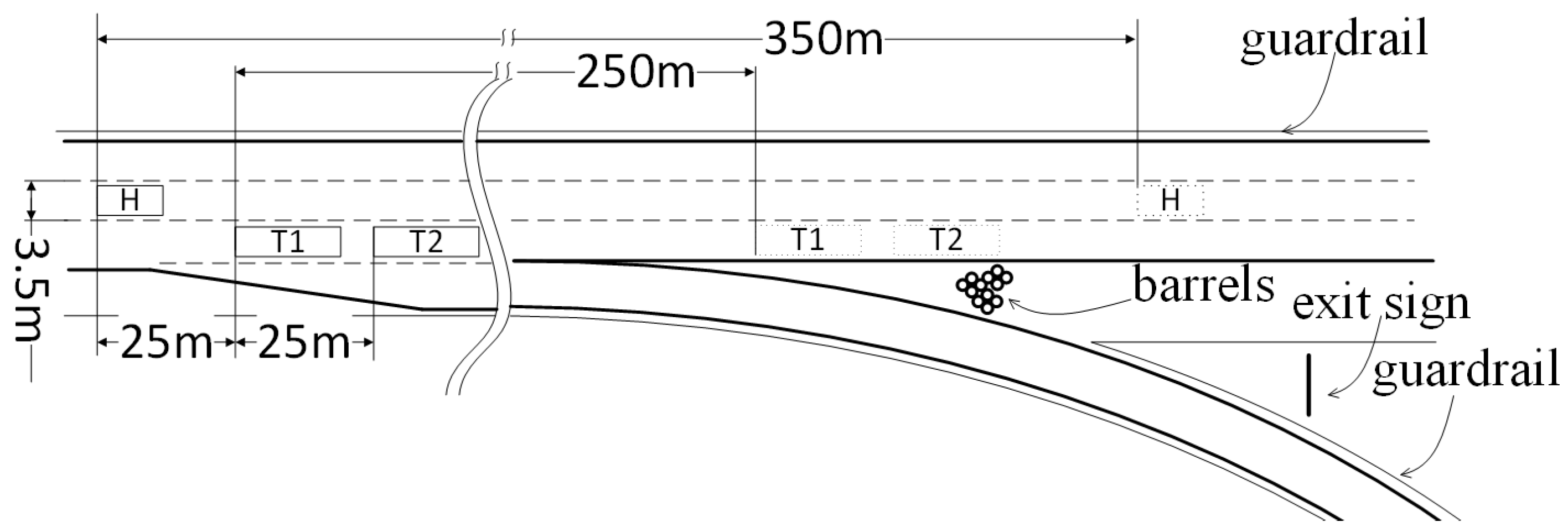
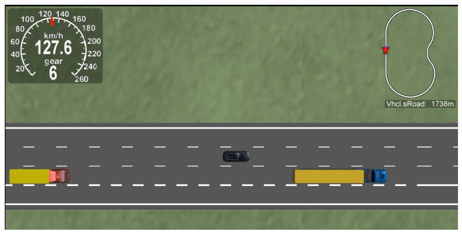
The experiment presented in this paper was performed using two test scenarios. Designed scenarios were chosen to represent highway situations to accurately represent intended-use cases of the perception system. Both scenarios were executed using the same virtual model (presented in Figure 1) of a straight section of the highway, bounded by guardrails on both sides, followed by an exit junction, with an exit sign and impact attenuating barrels. The test scenario models are shown in Figure 2 and Figure 3. Both scenarios assumed an approximately constant velocity of 126 km/h for the host vehicle along a straight line in the center lane. Scenario number 1 was executed with an empty road that did not contain any traffic participants except the host vehicle. Scenario number 2 contained one light and one heavy commercial vehicle in the right lane (Figure 4) moving with an approximately constant velocity of 90 km/h. In both scenarios, the host vehicle traveled 350 m over the duration of 10 s.
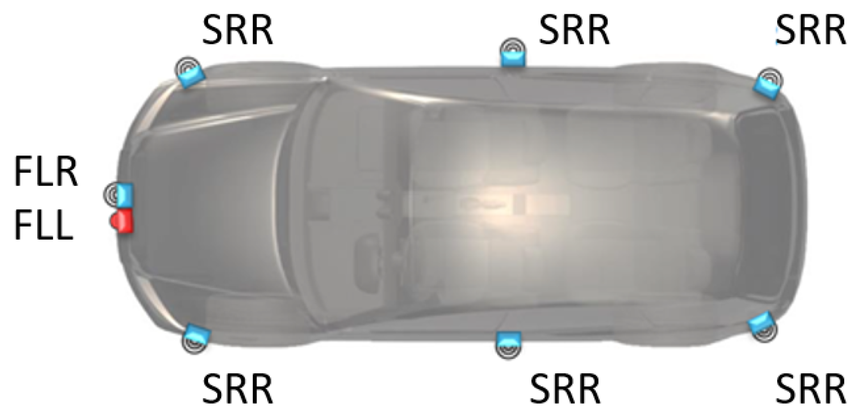
Figure 5 shows the sensors installed on the virtual validation vehicle that were modeled in the simulation tool. Sensor information was used for the parametrization of the sensor models. The sensor models were used to generate the point cloud that was used in further sensor modeling and reference data generation.
2.1. Framework Architecture
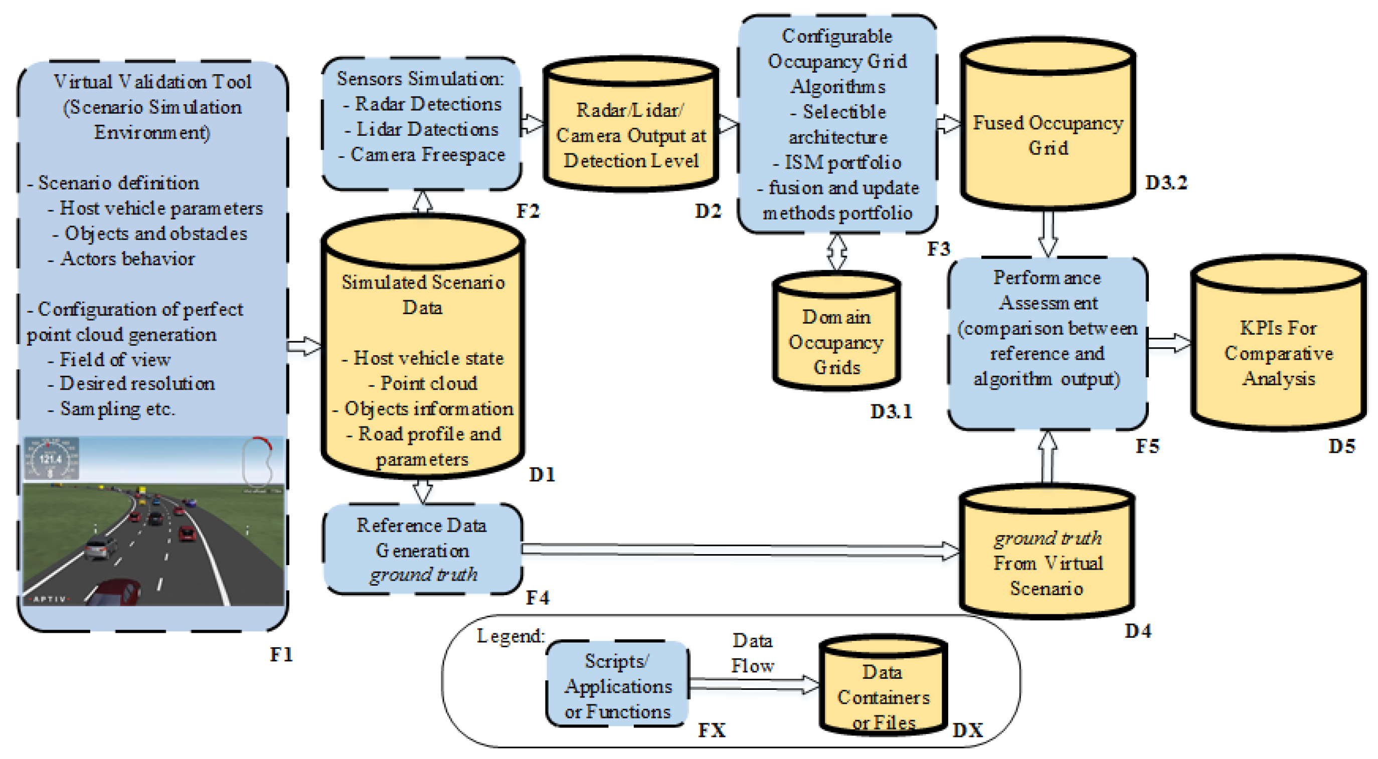
The general flow of data in the framework implemented in this study is presented in Figure 6.
2.2. Scenario and Point Cloud Generation
First, the traffic scenarios are defined, then modeled in the F1 module. Modeling of scenarios included definitions of traffic participants types and behaviors, planning of the the host vehicle speed profile and trajectory, as well as definition of stationary highway infrastructure and buildings. This step was performed using a commercial automotive simulation tool that incorporates modeling of the vehicle dynamics, actors behavior, and simplified sensor models.
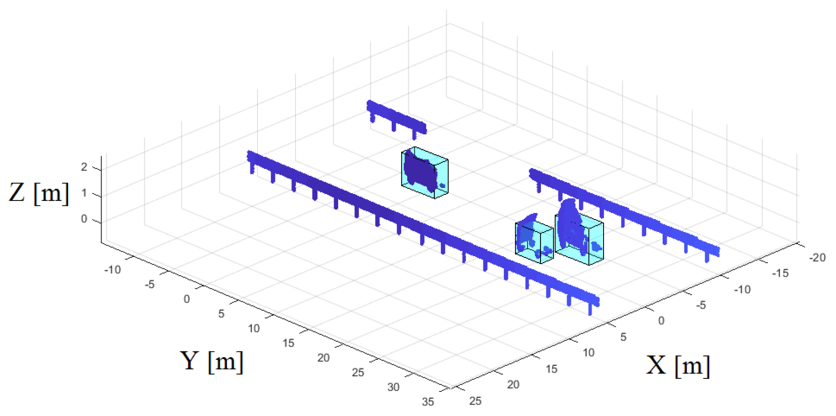
The simulation results incorporate object information, the detection points representing the environment (computed on a GPU using ray tracing), host vehicle motion and position, and parameters describing road curvature. A visualization of data D1 is shown in Figure 7.
2.3. Sensor Modeling
The purpose of modeling of the sensors is to obtain a realistic lidar and radar detection points using D1. The goal is achieved with the F2 component by parametrization of sensor pose on vehicle, temporal characteristics (detection interval and latency), velocity, position and azimuth accuracy. Calibration parameters are used to add noise to the scenario data [6]. Calibration parameters are based on the assessment of sensor performance in controlled conditions (anechoic chamber with reference target) similar to the method described for Aptiv ESR (Electronically Scanning Radar) [7]).
2.4. Occupancy Grid Framework
The implemented framework accommodates two fusion architectures: centralized or low/measurement-level and decentralized or grid-level [8]. Data and processes F3 D3.1 and D3.2 are described in this paragraph.
In the decentralized fusion, domain grid data container represented by D3.1 are used before fusing the grids. In this approach, intermediate caches of grid data were created for each domain. Table 1 contains the description of the variants and methods.
In the low-level mode, the reflection points and vehicle state information data D2 are utilized for computing data D3.2. Data caches were used to queue measurements from sensors and vehicle state.
2.4.1. Inverse Sensor Models
Inverse Sensor Models (ISM), are utilized in the process of the calculation of occupancy probability from the sensor measurements (lidar or radar reflection point). ISMs were utilized in this research to update the three sigma regions around the detection point.
This research used ISMs without ray-casting to compute the probability of occupancy in two-dimensional (2D) surroundings of the detection space. In some cases the “hit point” only approach was used to update just the single cell containing the detection. This approach is popular mainly in binary grids.
2.4.2. Occupancy Probability Calculation
The concept used in this experimental evaluation assumes that the probability of the existence of an obstacle is described by a Gaussian distribution. The ISMs presented for this application are required to operate for a 2D occupancy grid. This imposes a need to use a Bi-variate Normal Distribution function as the probability density function for the calculation of the occupancy probability of the affected cells. The second one is imposed by the sensors that supply the detection points (radar or lidar) with information about the position in 2D with respect to the Sensor Coordinate System (SCS) and and a covariance matrix for the detection. The ellipse simplification of a banana shape distribution is used due to the fact of relatively good azimuth resolution of evaluated sensors with respect to the detection range. Additionally, the detection contains information, such as existence probabilities .
The general formula used for the Probability Density Function (PDF) (2) requires a covariance matrix which describes variances and covariances with respect to the Occupancy Grid Coordinate System (OGCS).
where X contains a position in and (3) for the PDF values to be calculated.
Following , which in the general formula is the mean value of the distribution, in this case, determines the position of the detection in OGCS.
in addition to the co-variance matrix,
The sensors report data with respect to SCS. The position of SCS with respect to OGCS is known due to the fact that the sensor is mounted in a known location on the vehicle chassis and the vehicle position is tracked with respect to OGCS. The location in the simulation environment can be obtained directly from a built-in positioning component or in the case of real-world testing using a high fidelity INS (Inertial Navigation System). Therefore, a rotation matrix R and a translation vector T can be created to convert the information from SCS to OGCS.
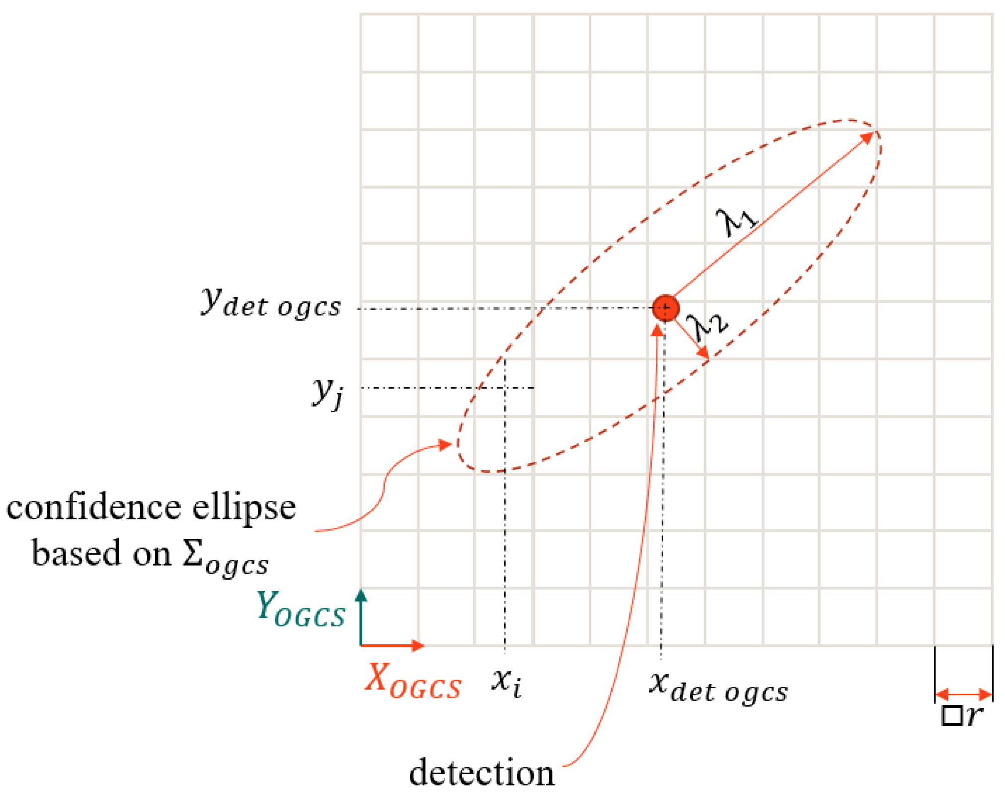
With all the input information, the computation of the probability for cells of the grid lying within a three-sigma ellipse (Figure 8) can be carried out by the integration of the PDF for each of the cells (10). The semi-minor and semi-major axes dimensions can be computed from the .
Eigenvalues and and eigenvectors and are calculated for the . Using this information, we can get the ellipse Equation (8), where s corresponds to the ellipse size.
The value of s can be computed from the desired confidence level for the area we want to update.
To find the orientation of the ellipse, the eigenvector corresponding to the maximum eigenvalue is used (9).
The ellipse obtained in these steps is used to select the cells of the grid lying inside of the ellipse in order to perform an update either by a lookup table with integration results or by numerically integrating the PDF of selected cell areas. The example of results numerical integration results is shown in Figure 9.
2.4.3. Fusing the Probability
The probability fusion methodology can be diversified in three ways:
- The first diversification comes from the Low and High Level architectures.
- The second diversification comes from the mathematical method used for the calculation of the output probability of occupancy. Grid-level fusion, distinguished the updated method from the fusion method, as it creates a sensor (domain) grid and then fuses them together. This results in the fact that a different method can be building the domain grid and different one can be fusing domains. The following section details methods identified in the literature, implemented in the framework and used for testing [8].
- The third diversification addresses the use of time filtering in building the input grid or use of instantaneous (single snapshot of one set of measurements—e.g., a list of radar detections from one scan) grid. This approach applies only to the High Level approach, where separate grids are created for sensors or domains. The Low Level grid, by nature, is a time filtered grid.
A detailed description of the fusion methods used in this study is given below.
- Bayesian Inference Filter (Bayes)The default approach for filtering in the presented case is the Bayes filter, since the occupancy grid in most prior work is based on Bayesian probability theory. The Bayesian filter is an extension of the Bayes estimator applied in cases where the observed values change over time [9]. Originally, the method finds application in the field of radar tracking to estimate beliefs about the recent position of targets [10]. The equation’s general form is (11), where is the posterior probability of occupancy given, are measurements and are host poses on the grid.However, with respect to future optimized software implementations, a logarithmic approach presented by Galvez is used where the given probability value is converted to the log-odds representation by means of Equation (12) [8].With the log-odds representation of both inverse sensor model output and the occupancy grid, fusion is performed by summing the log-odds values (13).The Bayes filter is then applied to every updated cell in the occupancy grid in the form of a log-odds ratio, which corresponds to performing a recursive Binary Bayes Filtering using the probability from the ISM. This approach tends to increase the a prior probability when the values exceed a 0.5 threshold and performs oppositely for values below that threshold. The issue is a correct effect from the statistics point of view, but it is causing problems in real applications of the methods, “dead locking” in the case of one input (grid cell or inverse sensor model output) reaching 0 or 1. To prevent this situation, a minimum and maximum probability saturation is set for the complete grid by a tuneable parameter. This parameter is used to offset the minimum and maximum values from 0 to, for instance, 0.1 and from 1 to 0.9.
- Dempster–Shafer (D-S)The Dempster–Shafer evidence theory is the second major mathematical apparatus employed in the task of building the occupancy grid. This method finds application in the area of tracking paths of moving targets for the estimation of both belief of existence and non-existence of false targets [10]. The primary advantage of this method over the Bayesian approach is the capability for explicit handling of the absence of information—e.g., an unknown state. The second crucial feature is the ability of the method to identify conflicting measurement information [11]. These advantages come with a cost that requires the definition of more than just the occupancy probability grid. Additional layers are needed to represent probability masses. Two mass matrices are needed—occupiedand emptyThe basis for computing of the cell probability is the Dempster–Shafer combination Formula (16).whereand the conversion of masses to probability is calculated byThe Dempster–Shafer combination formula applied to the occupancy grid gives the following formulas:The equations provide a final probability value obtained by the following approach:
- Linear Opinion Pool (LOP)The method identified in the literature [8] allows for the resolution of conflicting sensor information [12] based on an opinion pooling methodology [13]. An example application of the family of opinion pooling methods is pooling opinions from individuals for drawing conclusions (such as expert opinions) [14].This method assumes the existence of a weight that can represent the contribution of certain sensors [12].
- Independent Opinion Pool (IOP)A method which is based on the assumption that the sources are considered to be independent is a modification of the IOP.
- Logarithmic Independent Opinion Pool (LIOP)Another generalization of prior methods is a weighting process on top of probability distributions, which comes as a result of splitting the process into two steps: first, a weighted average, and second, a geometric weighted average [8].
- De Morgan’s Law (DeMorgan)Another approach proposed for fusing grids or measurement results inside grids is proposed by Galvez and has a tendency to favor higher probabilities [8]. This method has applications in text searching and it can be applied to simplify Boolean equations to the use of only AND and NOR gates.
- Maximum Policy (Max)
An in-depth description of these methods, along with lookup table plots, can be found in the work of Galvez [8]. In the remaining sections, evaluations taking into consideration qualitative results are presented.
2.5. Performance Assessment Methods
To compare the quality of discussed fusion methods, reference data D4 are created with the reference data generation tooling F4. Then it is compared with the analyzed algorithm set results D3.2 using KPI tooling F5. The analysis results are provided in a report D5, with performance indicators for a given set of input data.
2.5.1. Reference Data Generation
The objective of generating reference data is to obtain an idealistic representation of the test scenario. Therefore, a relatively high tessellation resolution of 0.05 m compared to 0.2 m in the fused grid is chosen. Cells in the high resolution reference grid that are physically occupied by stationary obstacles (barriers, vegetation, curbs, etc.) are flagged. As the analysis focuses on the static grid, footprints from dynamic objects are removed. In the end, the reference data grid is defined with a binary state (30).
The process of performance assessment is explained by a 1D simplification where both the reference and the computed grids, which normally consist of rectangular cells, are represented by line segments with given values. In Figure 10, a 1D simplification of a process of ground-truth (reference) grid creation based on the perfect sensor is presented. The assumption for the reference data is that, anywhere on the reference grid where there was a registered detection (from the reference sensor) above the road surface level, the binary occupancy state of that cell is set to true. This process is performed for the complete length of the tested scenario to accumulate the information using reference positioning information of the perfect sensor.
2.5.2. Proposed KPIs
Every resultant (the 1-D simplification is presented in Figure 10) cell is compared to ground-truth. The results of grid fusion D3.2 are binarized and undergo spatio-temporal alignment against the reference map D4. The results are classified as: True Positive (TP), True Negative (TN), False Positive (FP), and False Negative (FN). The number in a given class is added [17]. Then, the data are used for analysis with the following KPI methods:
- Probability of detectionThis indicator corresponds to the True Positive Rate (TPR) produced by the algorithm, and its increase means that the analyzed method is better at detecting actual obstacles, and is therefore expected to be maximized.
- PrecisionThe factor representing Positive Predictive Value (PPV) indicates how good the method is at judging whether the reported occupied areas are actually occupied. This factor is therefore expected to be maximized for the best performance.
- Probability Of False AlarmThe False Positive Rate (FPR) shows how bad the method is at the estimation of a certain cell as free when it is occupied in the scope of all those events and actually free cells in the experiment. For better performance, this factor has to be minimized, since the severity of false positives is significant in the Advanced Driver Assistance Systems from a functional safety perspective [18].
- False Discovery Rate (FDR)The FDR describes a ratio of how many cells identified as occupied were falsely classified. In terms of a better performing method, this factor must be minimized.
- F1 ScoreF1 Score is also known as a measure of accuracy, or a harmonic mean of precision and accuracy. The higher the value of this factor, the better the performance of the method.
- Normalized Occupied Map Score (NOMS)The NOMS method is a variation of the method used for grid performance evaluation proposed by Colleens et al. [19]. This method relies on non-binary algorithm outputs (a grid composed of cells with a probability gradient) A and a filtered reference grid B—obtained by subjecting a binary reference grid to a spatial filtering that generates gradients of probabilities. The maximization of the score for this method indicates higher performance.
The set of chosen indicators purposely does not include the methods relying heavily on true negatives due to the sparse nature of the grids. These kinds of indicators were identified as having a bias on the results.
3. Results
Experimental evaluation was performed using the configurations of the methods and the architectures. The results of this evaluation are presented in Table 1. The presented methods were run in both of the test scenarios (Scenario 1—without moving obstacles—and Scenario 2—including two moving targets). Reprocessing was carried out through the complete processing chain and resulted in the list of performance indicators presented in the bar plots in Figure 11.
Figure 11 presents the results for Scenario 1 and Scenario 2. The relation between a higher sensitivity of a method (having a higher True Positive Rate and Positive Predicted Value) and its susceptibility to false classification when subjected to clutter (having higher False Detection Rate and True Positive Rate) was observed. This is reflected in small differences of the F1 score. This relation can also be observed in the raw probability of occupancy presented in a form of snapshots in Figure 12 and Figure 13.
Overall, most of the methods have lower performance in Scenario 1 (visible in blue in Figure 11) compared to Scenario 2 (visible in red in Figure 11). This observation relates to the inability of the performance assessment method to explicitly handle occlusions and dynamic objects.
Looking at the results presented in the Figure 12, observations on practical aspects of the methods can be made. An important practical factor for all methods is that the obstacles, such as impact attenuating barrels, are properly reported by all the tested configurations, so this means that methods should satisfy simple object avoidance perception needs. In the cases of High Level Bayesian, Fused High Level Bayesian, Fused High Level Logarithmic Independent Opinion Pool and Fused High Level Independent Opinion Pool, we can see a tendency in the suppression of false occupancy in the right emergency lane, which is considered positive for the methods’ performances in applications, such as emergency trajectory planning. The mentioned methods, however, present much lower maximum range at which the occupancy from guardrails are accumulated, which can have a negative effect in case of application—i.e., for map matching.
During the course of the analysis of the probability representation presented in Figure 13, inconsistency in the occupied areas was identified in the right lane. Further investigation of the observed behavior led to the conclusion that deficiencies in the sensor simulation process resulted in false ground detection. Those deficiencies result in a reduction in reliability of the KPIs and create an opportunity for further development. The second observation related to the influence of sensor model “spreading” of probability influences the overall performance, depending on the method used for fusion. This indicates that the performance of given method could be adjusted by fine tuning or modifying the ISM.
4. Discussion
The research presented in this article investigated the use of an automotive virtual validation tool-chain for prototyping perception algorithms.
The key takeaways from the presented research indicate that the virtual tool-chain employed in this experiment allows:
- Early identification, testing, and definition of architectures and system level approaches.
- Quick development of the prototype software.
- Proofing of validation concepts.
- Early identification of architecture limitations.
- Integration and definition of the functional requirements when the hardware is not yet available.
- Extremely high scenario repeatability in comparison to real world testing.
- Generation of high precision reference data that would not be possible to obtain using a reference lidar mounted on a moving platform.
These features are crucial for complex system providers for the definition of products to better correspond with the customer’s technical needs.
The employed tool-chain will aid in the generation of dangerous scenarios—e.g., dense traffic, that would require vast effort and cost to be produced in the real world with controlled conditions. The tool-chain can also help in the definition of KPIs (Key Performance Indicators) and the validation of their reliability.
The limitations of this approach are related to its ability to realistically represent the critical properties of test scenarios and sensors. Those limitations, however, underline that the final validation and performance assessment of more technically mature products requires the extensive use of real data.
Virtual validation frameworks will benefit from increasing the realism of sensor models, which will lead to the more widespread adoption of virtual validation in perception algorithm development. The reduced ability to represent physical phenomenon in the evaluated simulation process decreased the reliability of the proposed performance assessment scheme. This was reflected in the fact that a set of numerical KPIs has been identified to be not consistent with expert assessment. Numerical results obtained from the comparison indicate that the higher the sensitivity of the method, the more prone it is to clutter and noise. A valid testing methodology requires tailoring depending on the application of the perception module to yield useful results.
The solution used as a module F3 did undergo testing in a real world environment. The results of the real world tests will be used as the subject of further dissemination, including a comparison of results between simulated and real environments.
Author Contributions
Conceptualization, P.M. and J.P.; methodology, P.M.; software, J.P.; validation, J.P.; formal analysis, P.M.; investigation, P.M.; resources, P.M.; data curation, P.M.; writing—original draft preparation, P.M.; writing—review and editing, P.M.; visualization, P.M. and J.P.; supervision, P.M.; project administration, P.M.; funding acquisition, P.M. and J.P. All authors have read and agreed to the published version of the manuscript.
Funding
Research funded by Polish Ministry of Science and Higher Education (MNiSW) contract number: 10/DW/2017/01/1.
Conflicts of Interest
The authors declare no conflict of interest.
References
- Markiewicz, P.; Kogut, K.; Róźewicz, M.; Skruch, P.; Starosolski, R. Occupancy Grid Fusion Prototyping Using Automotive Virtual Validation Environment. In Proceedings of the 6th International Conference on Control, Mechatronics and Automation, ICCMA, Tokyo, Japan, 12–14 October 2018; ACM: New York, NY, USA, 2018; pp. 81–85. [Google Scholar] [CrossRef]
- Elfes, A.; Matthies, L. Sensor integration for robot navigation: Combining sonar and stereo range data in a grid-based representataion. In Proceedings of the 26th IEEE Conference on Decision and Control, Los Angeles, CA, USA, 9–11 December 1987; Volume 26, pp. 1802–1807. [Google Scholar] [CrossRef]
- Porebski, J.; Kogut, K.; Markiewicz, P.; Skruch, P. Occupancy grid for static environment perception in series automotive applications. IFAC-PapersOnLine 2019, 52, 148–153. [Google Scholar] [CrossRef]
- Jungnickel, R.; Kohler, M.; Korf, F. Efficient automotive grid maps using a sensor ray based refinement process. In Proceedings of the 2016 IEEE Intelligent Vehicles Symposium (IV), Gothenburg, Sweden, 19–22 June 2016; pp. 668–675. [Google Scholar] [CrossRef]
- Skruch, P.; Dlugosz, R.; Kogut, K.; Markiewicz, P.; Sasin, D.; Rozewicz, M. The Simulation Strategy and Its Realization in the Development Process of Active Safety and Advanced Driver Assistance Systems; SAE Technical Paper; SAE International: Warrendale PA, USA, 2015. [Google Scholar] [CrossRef] [Green Version]
- Wang, Z.; Yi, D.; Duan, X.; Yao, J.; Gu, D. Measurement Data Modeling and Parameter Estimation; CRC Press: Boca Raton, FL, USA, 2012; p. 290. [Google Scholar]
- Stanislas, L.; Peynot, T. Characterisation of the Delphi Electronically Scanning Radar for robotics applications. In Proceedings of the Australasian Conference on Robotics and Automation (ACRA 2015), Canberra, Australia, 2–4 December 2015. [Google Scholar]
- Galvez del Postigo Fernandez, C. Grid-Based Multi-Sensor Fusion for On-Road Obstacle Detection: Application to Autonomous Driving. Master’s Thesis, (Master of Science in Systems, Control and Robotics). KTH Royal Institute of Technology, School of Computer Science And Communication, Stockholm, Sweden, 2015. [Google Scholar]
- Arulampalam, M.S.; Maskell, S.; Gordon, N.; Clapp, T. A tutorial on particle filters for online nonlinear/non-Gaussian Bayesian tracking. IEEE Trans. Signal Process. 2002, 50, 174–188. [Google Scholar] [CrossRef] [Green Version]
- Bar-Shalom, Y.; Willett, P.; Tian, X. Tracking and Data Fusion: A Handbook of Algorithms; YBS Publishing: Storrs, CT, USA, 2011. [Google Scholar]
- Siegel, M.; Stiefelhagen, R.; Yang, J. fusion using Dempster–Shafer theory [for context-aware HCI]. In Proceedings of the 19th IEEE Instrumentation and Measurement Technology Conference, Anchorage, AK, USA, 21–23 May 2002; Volume 1, pp. 7–12. [Google Scholar] [CrossRef]
- Adarve, J.D.; Perrollaz, M.; Makris, A.; Laugier, C. Computing Occupancy Grids from Multiple Sensors using Linear Opinion Pools. In Proceedings of the IEEE International Conference on Robotics and Automation, Saint Paul, MN, USA, 14–18 May 2012. [Google Scholar]
- Degroot, M.H. Reaching a Consensus. J. Am. Stat. Assoc. 1974, 69, 118–121. [Google Scholar] [CrossRef]
- Bradley, R. Learning from others: Conditioning versus averaging. Theory Decis. 2018, 85, 5–20. [Google Scholar] [CrossRef]
- Muhamad Abdulghafour, M.A.A. Data fusion through nondeterministic approaches: A comparison. SPIE 1993, 2059. [Google Scholar] [CrossRef]
- Thrun, S.; Burgard, W.; Fox, D. Probabilistic Robotics (Intelligent Robotics and Autonomous Agents); The MIT Press: Cambridge, MA, USA, 2005. [Google Scholar]
- Carvalho, J.; Ventura, R. Comparative Evaluation of Occupancy Grid Mapping Methods Using Sonar Sensors. In Pattern Recognition and Image Analysis; Sanches, J.M., Micó, L., Cardoso, J.S., Eds.; Springer: Berlin/Heidelberg, Germany, 2013; pp. 889–896. [Google Scholar]
- ISO. Road Vehicles—Functional Safety; ISO: Geneva, Switzerland, 2011. [Google Scholar]
- Colleens, T.; Colleens, J.J.; Ryan, D. Occupancy grid mapping: An empirical evaluation. In Proceedings of the 2007 Mediterranean Conference on Control Automation, Athens, Greece, 27–29 June 2007; pp. 1–6. [Google Scholar] [CrossRef]
Figure 1.
Schematics of the scenario modeled in the environment (H—host vehicle; T1, T2—target vehicles. Solid line indicates initial and dotted final positions).
Figure 1.
Schematics of the scenario modeled in the environment (H—host vehicle; T1, T2—target vehicles. Solid line indicates initial and dotted final positions).

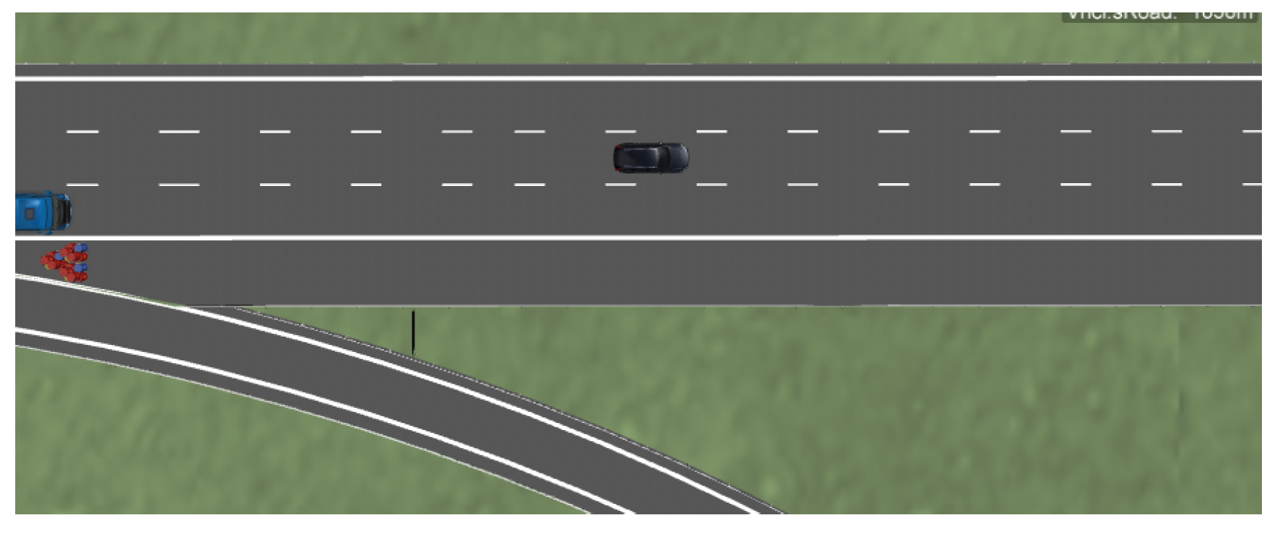
Figure 2.
Snapshot of the junction in the test environment.

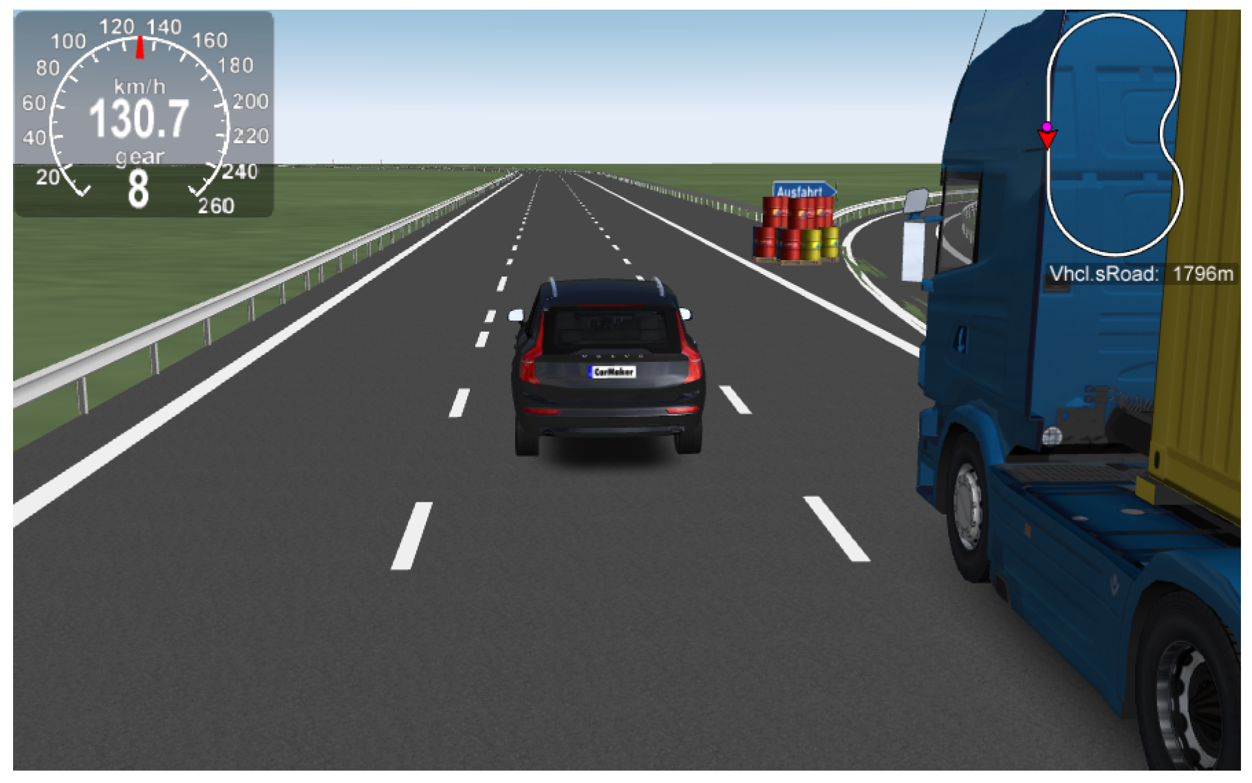
Figure 3.
Snapshot of the junction, exit sign, and impact attenuating barrels.

Figure 4.
Snapshot of the scenario, including two commercial vehicles.

Figure 5.
Sensor suite on the vehicle model (SRR—Short Range Radar; FLR— Forward Looking Radar; FLL—Forward Looking Lidar).
Figure 5.
Sensor suite on the vehicle model (SRR—Short Range Radar; FLR— Forward Looking Radar; FLL—Forward Looking Lidar).

Figure 6.
The Framework Schematics and Data Flow.

Figure 7.
Modeled detection from stationary infrastructure (barriers) and dynamic target vehicles (in bounding boxes).
Figure 7.
Modeled detection from stationary infrastructure (barriers) and dynamic target vehicles (in bounding boxes).

Figure 8.
Confidence ellipse around the detection with semi-major axis a, semi-minor axis b, and center coordinates , of the cell .
Figure 8.
Confidence ellipse around the detection with semi-major axis a, semi-minor axis b, and center coordinates , of the cell .

Figure 9.
Computed result of the probability density function integrated on the grid.

Figure 10.
Drawing of the 1D simplification of the reference data generation and comparison with the high resolution reference data along with the resulting event classification for the performance assessment.
Figure 10.
Drawing of the 1D simplification of the reference data generation and comparison with the high resolution reference data along with the resulting event classification for the performance assessment.

Figure 11.
Colored bar plots of KPI results per scenario. TPR—True Positive Rate, PPV—Positive Predicted Value, F1 Score, FPR—False Positive Rate, FDR—False Detection Rate, NOMS—Normalized Occupancy Map Score.
Figure 11.
Colored bar plots of KPI results per scenario. TPR—True Positive Rate, PPV—Positive Predicted Value, F1 Score, FPR—False Positive Rate, FDR—False Detection Rate, NOMS—Normalized Occupancy Map Score.

Figure 12.
Snapshots of resultant occupancy grid for fusion variants in the first row: LL-B, LL-DS, HL-B, HL-M, HL-LI, HL-L, HL-I; in the second row: HL-De, HL-S, FHL-B, FHL-LI, FHL-L, FHL-I for Scenario 1).
Figure 12.
Snapshots of resultant occupancy grid for fusion variants in the first row: LL-B, LL-DS, HL-B, HL-M, HL-LI, HL-L, HL-I; in the second row: HL-De, HL-S, FHL-B, FHL-LI, FHL-L, FHL-I for Scenario 1).

Figure 13.
Snapshots of resultant occupancy grid for fusion variants in the first row: LL-B, LL-DS, HL-B, HL-M, HL-LI, HL-L, HL-I; in the second row: HL-De, HL-S, FHL-B, FHL-LI, FHL-L, FHL-I for Scenario 2).
Figure 13.
Snapshots of resultant occupancy grid for fusion variants in the first row: LL-B, LL-DS, HL-B, HL-M, HL-LI, HL-L, HL-I; in the second row: HL-De, HL-S, FHL-B, FHL-LI, FHL-L, FHL-I for Scenario 2).


Table 1.
Tested configurations and their naming.
| Variant Abbreviation | Variant Full Name | Architecture Variant | Filtering Mode | Method |
|---|---|---|---|---|
| LL-B | Low Level Bayes | Low | Accumulated | Bayes |
| LL-DS | Low Level Dempster–Shafer | Low | Accumulated | D-S |
| HL-B | High Level Bayes | High | Instantaneous | Bayes |
| HL-M | High Level Max | High | Instantaneous | Max |
| HL-LI | High Level Logarithmic Independent Opinion Pool | High | Instantaneous | LIOP |
| HL-L | High Level Logarithmic Opinion Pool | High | Instantaneous | LOP |
| HL-I | High Level Independent Opinion Pool | High | Instantaneous | IOP |
| HL-De | High Level DeMorgan | High | Instantaneous | DeMorgan |
| HL-S | High Level Sum | High | Instantaneous | Sum |
| FHL-B | Fused High Level Bayes | High | Accumulated | Bayes |
| FHL-LI | Fused High Level Independent Opinion Pool | High | Accumulated | LIOP |
| FHL-L | Fused High Level Logarithmic Opinion Pool | High | Accumulated | LOP |
| FHL-I | Fused High Level Independent Opinion Pool | High | Accumulated | IOP |
Publisher’s Note: MDPI stays neutral with regard to jurisdictional claims in published maps and institutional affiliations. |
© 2020 by the authors. Licensee MDPI, Basel, Switzerland. This article is an open access article distributed under the terms and conditions of the Creative Commons Attribution (CC BY) license (http://creativecommons.org/licenses/by/4.0/).
Share and Cite
MDPI and ACS Style
Markiewicz, P.; Porębski, J. Developing Occupancy Grid with Automotive Simulation Environment. Appl. Sci. 2020, 10, 7629. https://0-doi-org.brum.beds.ac.uk/10.3390/app10217629
AMA Style
Markiewicz P, Porębski J. Developing Occupancy Grid with Automotive Simulation Environment. Applied Sciences. 2020; 10(21):7629. https://0-doi-org.brum.beds.ac.uk/10.3390/app10217629
Chicago/Turabian StyleMarkiewicz, Paweł, and Jakub Porębski. 2020. "Developing Occupancy Grid with Automotive Simulation Environment" Applied Sciences 10, no. 21: 7629. https://0-doi-org.brum.beds.ac.uk/10.3390/app10217629
Note that from the first issue of 2016, this journal uses article numbers instead of page numbers. See further details here.