Article

Modelling of the Acetification Stage in the Production of Wine Vinegar by Use of Two Serial Bioreactors

by
Carmen M. Álvarez-Cáliz
1,
Inés María Santos-Dueñas
1,*,
Jorge E. Jiménez-Hornero
2 and
Isidoro García-García
1
1
Department of Chemical Engineering, Campus de Rabanales, University of Cordoba, 14071 Cordoba, Spain
2
Department of Electrical Engineering and Automatic Control, Campus de Rabanales, University of Cordoba, 14071 Cordoba, Spain
*
Author to whom correspondence should be addressed.
Submission received: 28 November 2020 / Revised: 12 December 2020 / Accepted: 16 December 2020 / Published: 18 December 2020

Abstract

:
In the scope of a broader study about modelling wine acetification, the use of polynomial black-box models seems to be the best choice. Additionally, the use of two serially arranged bioreactors was expected to result in increased overall acetic acid productivity. This paper describes the experiments needed to obtain enough data for modelling the process and the use of second-order polynomials for this task. A fractional experimental design with central points was used with the ethanol concentrations during loading of the bioreactors, their operation temperatures, the ethanol concentrations at unloading time, and the unloaded volume in the first one as factors. Because using two serial reactors imposed some constraints on the operating ranges for the process, an exhaustive combinatorial analysis was used to identify a working combination of such ranges. The obtained models provided highly accurate predictions of the mean overall rate of acetic acid formation, the mean total production of acetic acid of the two-reactor system, and ethanol concentration at the time the second reactor is unloaded. The operational variables associated with the first bioreactor were the more strongly influential to the process, particularly the ethanol concentration at the time the first reactor was unloaded, the unloaded volume, and the ethanol concentration when loading.

1. Introduction

Vinegar production is a biotechnological process essentially involving the biological conversion of ethanol from a given source into acetic acid. Vinegar can be obtained from alcohol, wine, cereals or fruits, among other sources [1,2,3,4]. The key step of the process is possibly that by which a complex microbiota of acetic acid bacteria (AAB) convert ethanol into acetic acid in a bioreactor. The bacterial mixture affecting the conversion arises from the natural microbial selection in the acetification medium. In practice, only AAB can exist in an environment containing medium concentrations of ethanol and acetic acid at the beginning but low levels of the former and high levels of the latter at the end [5]. These conditions make it unnecessary to sterilize containers or keep aseptic conditions during operation.
Acetification bioreactors usually operate in a semi-continuous mode. Thus, once the reactors are in full operation, the ethanol concentration is allowed to decrease to a preset level and then an also preset fraction of the reactor contents is unloaded, the remainder being allowed to stand in it in order to act as an inoculum in the next conversion cycle [6,7,8,9,10]. After the bioreactor is unloaded, it is slowly replenished with a fresh alcoholic substrate to start a new ethanol depletion cycle.
Because the temperature and airflow rate are usually fixed, the operational variables that can be altered include the ethanol concentration at the time the reactor is unloaded, the proportion of broth that is unloaded, the loading mode and/or rate, and the total concentration of the culture medium—which is the combination of the ethanol concentration in % v/v and the acidity in % w/v [11,12,13,14,15,16]. These variables influence the mean ethanol concentration and acidity in each cycle [8,9,10], which in turn affect the AAB concentration and cell activity [17,18]. As a result, the acetification conditions will be more or less stressful for the bacteria affecting the process (AAB).
Usually, an acetification bioreactor is operated in an automated manner in order to not alter the spontaneous dynamics of the system. In practice, this allows repeated cycling to be easily and rapidly achieved [19]. Also, the characteristics of AAB [20,21,22,23] make cultivation and selection outside their typical natural or industrial environment rather difficult. In addition, their complex identification, behaviour, and interactions, and their potential synergistic effects, require determining their optimum conditions of operation in an empirical manner.
Notwithstanding the previous difficulties, there is a wealth of technical experience and knowledge about the most suitable working methods and operating conditions for acetification. The use of non-segregated non-structured models [24] could be appropriated to model this kind of system; working with this type of approach allowed us to reach most of the knowledge on this particular process, which has allowed quantitative relations between operational variables and diverse industrial objective functions such as productivity to be established [8,9,10,25,26,27,28,29,30].
The advent of massive methods of analysis, such as several omic techniques, has considerably expanded available knowledge about the acetification process at the molecular level, and is bound to help improve the stability and food safety of the end-product [31]. There is, however, an ongoing search for more or less structured modelling approaches to relating the variables of the overall process.
Previous modelling studies [7,10,30] led to proposing the use of two serially arranged bioreactors to optimize the outcome of the acetification process under operationally restricted conditions. Thus, vinegar production is most often subjected to strict regulations with regards to the properties of the end-product, which, for example, should contain very little or no ethanol. In practice, however, ethanol in the acetification medium should never be depleted before the reactor is unloaded since that would place AAB under extremely stressful conditions (viz., a high acidity and a lack of substrate) and render them virtually useless in subsequent biomass conversion cycles. As a result, many industrial acetification plants use additional bioreactors to deplete ethanol present in the vinegar following the unloading of the production bioreactors.
In this scenario, modelling of the two serial bioreactors system requires the use of an appropriate experimental design. Previous experience with modelling of the biotransformation stage in the vinegar production process suggests that black-box models based on second-order generalized polynomials [7,19,32,33,34] provide a more accurate depiction of the experimental results than do existing alternatives, allowing it to describe potential interactions between independent variables to be considered—and with added advantages like ease of development and statistical validation. The number of experiments needed for the accurate fitting of a polynomial equation depends on whether the polynomial is linear or non-linear [35]. In any case, the greater the number of polynomial terms is (increasing the accuracy of the model), the more experiments will be required to calculate their coefficients. All testing should be conducted in the framework of an experimental design using the minimum possible number of runs to identify interactions between variables and allowing representative equations for the target process to be established as possible.
Based on the previous comments, the main aim of this work was to obtain polynomial models for several key variables of the two serially arranged bioreactors system and to determine an appropriate experimental design for gathering the experimental data needed to estimate such models. A fractional factorial design with central points including the six major operational variables involved on the acetification process has been used, considering the fulfilment of several restrictions arising from the operation of the two bioreactors, which required identifying and examining the impact of such variables (specifically, establishing their lower and upper limits in the framework of the experimental design). Once the experiments were conducted, polynomial models of relevant target variables of the process such as productivity, acetification rate, etc. were fitted using the gathered experimental data. As far as we know, this thorough study where a detailed analysis considering the constraints for the operational variables, the so many experiments, as well as the replications carried out for each experimental set of variables’ values has not been done before; additionally, the modelling approach for this acetification set-up has not been reported in any other previous work.

2. Materials and Methods

2.1. Operating Mode

A diagram showing the operation of two bioreactors working serially is depicted in Figure 1, where the process involved the following operations:
  • Once the ethanol concentration in the first reactor was reduced to E u 1 , a volume fraction of culture medium V u 1 was unloaded, whereas the remainder was used as inoculum for the fresh medium to be loaded in order to replace the unloaded fraction. Immediately before the first reactor was partially unloaded, the second was completely unloaded in order to receive the portion withdrawn from the first.
  • Both reactors were loaded with fresh substrate (wine) controlling the ethanol concentrations to E l 1 in the first and E l 2 in the second. This allowed drastic changes in the ethanol and acetic acid concentrations to be avoided. In fact, intermittently adding appropriate amounts of fresh substrate allowed a constant concentration of ethanol to be maintained throughout the loading stage.
  • Once loading was finished, both reactors continued to operate until the second was again unloaded prior to the first.
This scheme allowed the following operational variables to be changed: ethanol concentration at the time the first reactor was unloaded ( E u 1 ), volume unloaded from the first reactor ( V u 1 ), the ethanol concentration while the first and second reactor were loaded ( E l 1 and E l 2 , respectively), and the temperature in each reactor ( T 1 and T 2 , respectively). A total of six operational variables were thus involved. Although the alcoholic strength of the wine and the airflow rate could also have been used as variables, the feed wine usually contains 12% (v/v) ethanol, and the airflow rate is usually as high as possible (especially when productivity is to be maximized). Also, using gas condensers minimized the sweeping of volatiles.
Except for the temperatures, the working range for the previous variables could not be freely chosen because each variable was subjected to physical limitations, especially because the serial operation of the two reactors imposed constraints arising from the mutual relationships between the variables. This required careful planning of the experimental work in order to define the number of experiments needed to obtain accurate information with a view to predicting the influence of each variable on the resulting system behavior. As described in Section 3.1, a fractional factorial design for this purpose was used [36].

2.2. Experimental Set-Up

Figure 2 shows the two serially arranged bioreactors used to conduct the experiments. The reactors were two 8 L Acetators from Heinrich Frings GmbH & Co. KG (Rheinbach, Germany) equipped with self-aspirating turbines in the bottom in order to obtain a dispersion of fine air bubbles. The reactors were highly efficient in transferring oxygen between the gas phase and the substrate [11]. The ensemble was interfaced to a computer for automated operation, especially with regards to loading and unloading of reactors, and monitoring of the process. This resulted in highly reproducible loading and unloading, and in efficient acquisition of data [6,11,37].

2.3. Raw Material

The substrate used was white wine from the Montilla–Moriles D.O. (Córdoba, Spain) containing (11.5 ± 0.5)% (v/v) ethanol and an initial acidity of (0.4 ± 0.1)% (w/v) as acetic acid.

2.4. Microorganisms

The inoculum used was a mixed culture of acetic acid bacteria (AAB) obtained from bioreactors previously operating in repeated acetification cycles with the same type of wine as the substrate. This is the usual mode of operation for the vinegar industry.

2.5. Analytical Methods

The only variable not determined automatically was acidity, which was measured by acid—base titration with an NaOH solution approximately 0.5 N that was previously standardized with potassium hydrogen phthalate. The volume and ethanol concentration were measured in a continuous manner by using an EJA 110 differential pressure probe from Yokogawa Electric Corp. (Tokyo, Japan) and an Alkosens probe equipped with an Acetomat transducer from Heinrich Frings, respectively.

2.6. Mathematical Methods

2.6.1. Polynomial Models and Fitting Methods

The models used here were based on second-order non-linear polynomial equations of the following type:
Y =   b 0 +   i = 1 n b i · X i +   i = 1 i < j n b i j · X i · X j +   i = 1 n b i i · X i 2 ,
where Y denotes the dependent variable, b 0 the independent regression term, b i the coefficients of the linear (first-order) terms, b i j those of non-linear (interaction) terms, b i i those of quadratic terms, X i the independent variables, X j the independent variables with i < j , and n the number of independent variables. The Y variable is the response or output of the polynomial model and X variables are the inputs.
The equations were fitted by using one of several specific methods along with experimental data to calculate the previous coefficients. Such methods allow identifying those terms in Equation (1) that are significant and those that are not. In practice, they solve a least-squares problem by minimizing the sum of squares of the residuals (prediction errors). Second-order polynomial models can be fitted by using several methods [38,39,40,41,42,43]. In this work, the Forward Stepwise Regression method has been used, which successively incorporates one by one those independent variables that contribute to predicting a dependent variable from the most to the least predictive. The sequence in which terms are added to or removed from a polynomial in each step of the process is established according to the F-to-enter, F-to-remove (reference values set by the modeler for the F-values associated to each term of the model), R and R2 criteria. Then, the F-statistics also give a measure of the model sensitivity to each term of the polynomial relating the input variables.

2.6.2. ANalysis Of VAriance (ANOVA)

Before the model equations were fitted, the experimental data to be used for this purpose were checked for statistical differences by analysis of variance (ANOVA), which compares the means for two or more data samples in terms of their variances. ANOVA’s null hypothesis is that all means are identical and the alternative hypothesis that at least one mean will be different from all others [36]. ANOVA is used to identify sources of differences among data samples and to assess whether the differences among sample media are too large to be assigned to random errors alone [44].

3. Results and Discussion

3.1. Experimental Design

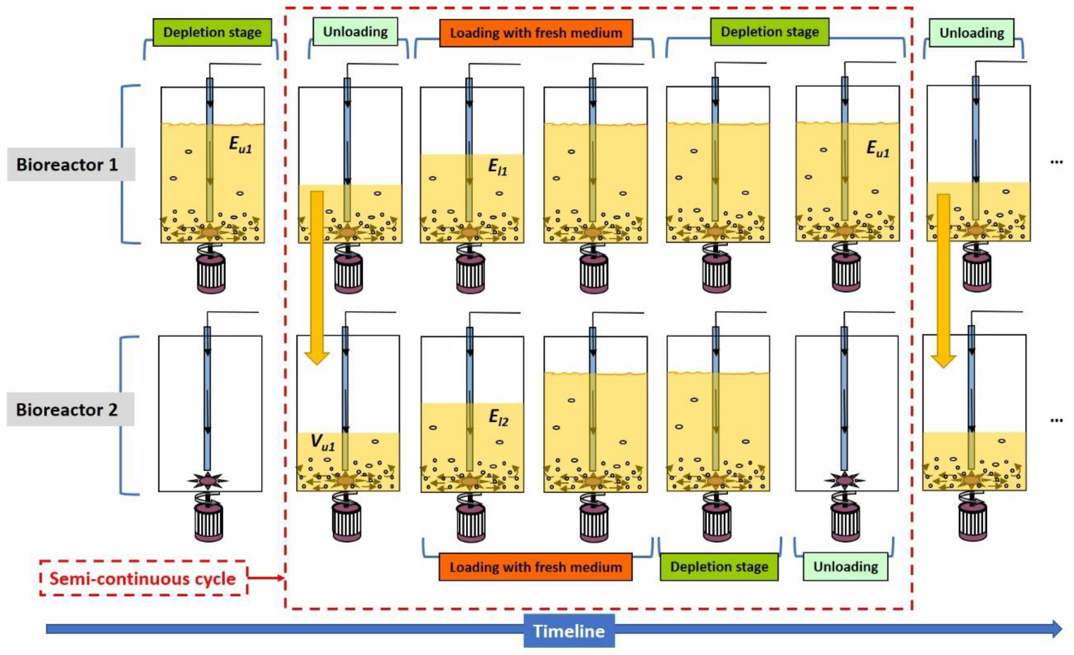
The experimental design that was initially intended to use was a Box-Behnken or Doehlert central composite factorial design. With two levels per factor, the total number of experiments needed was 2 n + 2 n + 1 , where the first term represents the overall factorial design, the second the central points of the faces, and the third the central point. The factors (operational variables) used were the ethanol concentration at the loading stage in the first bioreactor ( E l 1 ), the ethanol concentration at unloading time in the first bioreactor ( E u 1 ), the volume unloaded from the first bioreactor into the second one ( V u 1 ), the working temperature in the first bioreactor ( T 1 ), the ethanol concentration at loading time in the second bioreactor ( E l 2 ), and the working temperature in the second bioreactor ( T 2 ). A total of 77 different experiments were in theory needed for to model these operational variables. In practice, however, this would have involved too many runs—probably more than needed to fit the model. Also, each experiment would have to be replicated many times to obtain reproducible results and lag phases would be needed each time the operational variables were modified to investigate a new case.
It was therefore necessary to reduce the number of experiments without sacrificing experimental information. This was accomplished by using a fractional factorial design requiring only 2 n p experiments, where n is the total number of variables and p the number of those variables obtained from some interactions of the others. Thus, considering p = 2 (variables T 1 and T 2 ) and design generators I 1 = V u 1 · E u 1 · E l 1 and I 2 = V u 1 · E u 1 · E l 2 for a 1/4 fraction design, the experimental setup is shown in Table 1. Normalized values −1 and +1 have been used for V u 1 , E u 1 , E l 1 , E l 2 and columns for T 1 , T 2 have been obtained using I 1 , I 2 generators, respectively. For example, normalized values for T 1 were the product of normalized values of V u 1 , E u 1 and E l 1 ; similarly, normalized values for T 2 were the product of normalized values of V u 1 , E u 1 and E l 2 .
It was thought essential to use more than one central experiment (level 0 of all operational variables) at different times in order to examine the variance of the response variables. In this work, we used two central experiments (see Table 2). We would also use far-spaced experiments (levels −2 and +2) symmetrically placed at a distance α from center, α being the fourth root of the number of fractional factorial design experiments excluding central points (i.e., α = 16 4 = 2 ). Therefore, the distance of levels (−2) and (+2) from level (0) was twice that from (0) to (−1) and (+1). This required adding two experiments per operational variable (see Table 3). In summary, a total of 30 experiments would be required with the proposed design (i.e., less than one-half those required by a pure factorial design), with the added advantage that the ranges of operating conditions would be extended to far extreme values.
Because of the serial operation of the two bioreactors, several specific constraints must be considered for previous variables, since they cannot take certain values in practice:
Constraints on E l 1 :
  • The ethanol concentration of the feed wine would invariably be 12% (v/v).
  • E l 1 E u 1 as it would make no sense to have an ethanol concentration at the reactor loading stage lower than that at unloading time.
  • E l 1 must be less than the maximum ethanol concentration in the first bioreactor ( E l 1 ) m a x at any time. The latter concentration depends on E u 1 , V u 1 and the ethanol concentration of the feed wine, and can be calculated from the following mass balance:
    ( E l 1 ) m a x = ( 8 V u 1 ) · E u 1 + V u 1 · 12 8 ,
Constraints on E u 1 :
  • E u 1 must be greater than 1% (v/v) in order to prevent ethanol depletion from happening too early in the first bioreactor—the second bioreactor was used for this purpose. Also, too low a value would slow down acetification and decrease productivity as a result [15].
  • E u 1 must not be too high. Otherwise, ethanol not consumed in the first bioreactor would have to be used in the second and the probability of complete depletion before unloading would be diminished. Also, ethanol concentrations higher than 5–6% (v/v) could detract from microbial activity [15,45]. Therefore, E u 1 must not exceed 5% (v/v).
  • E u 1 < ( E l 1 ) m a x   (Equation (2)).
Constraints on V u 1 :
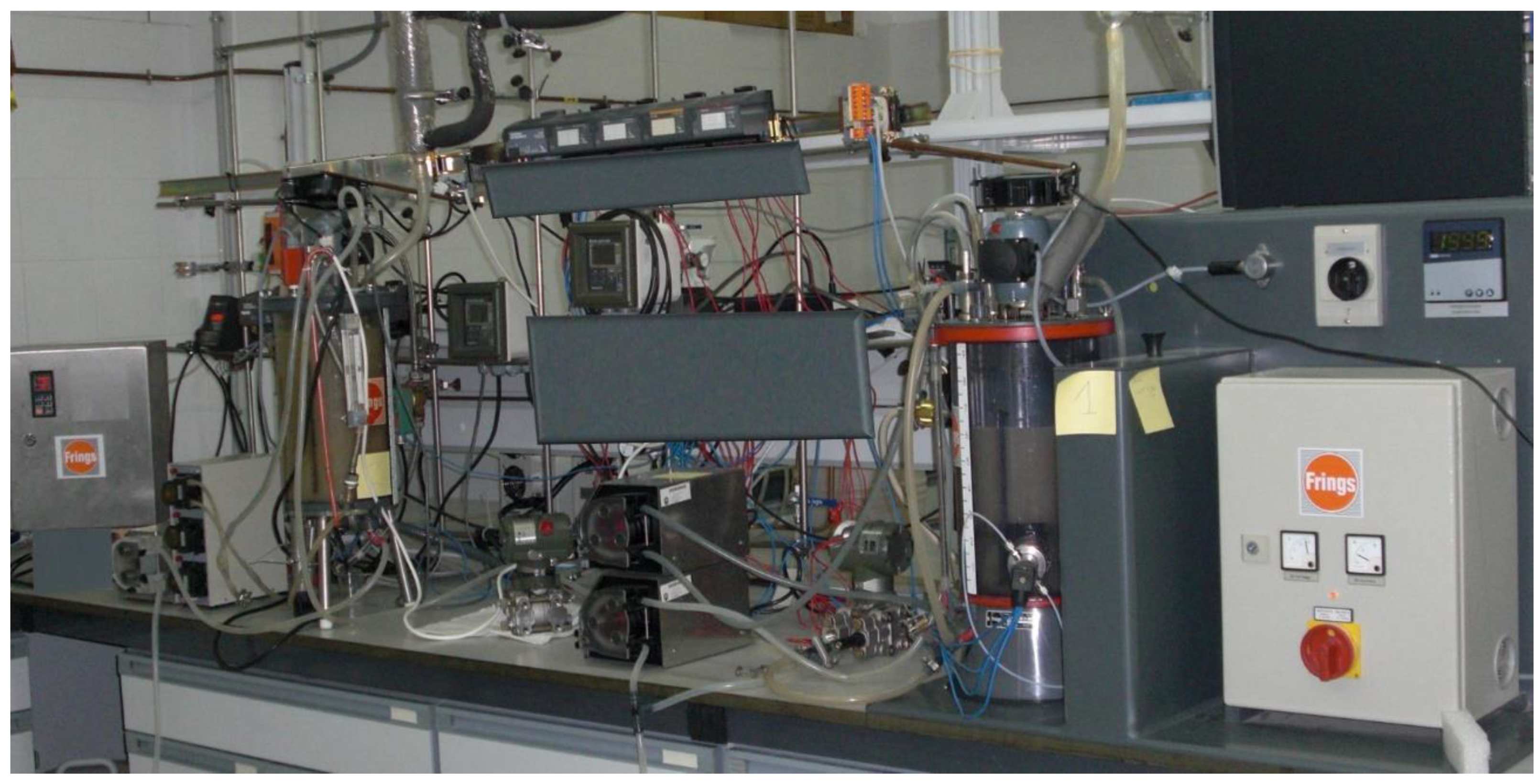
This variable must range from 1 to 7 L if the self-aspirating turbine with which the bioreactors were equipped is to operate properly. The turbine was used to feed oxygen to the microorganisms and help homogenize the culture medium.
Constraints on T 1 and T 2 :
The values of these variables must be compatible with the activity of acetic acid bacteria (AAB), which are the microorganisms affecting the process. The optimum temperature for AAB to oxidize ethanol into acetic acid is 25–35 °C. Because AAB activity drops outside this range [46,47], temperatures from 26 to 34 °C have been used here.
Constraints on E l 2 :
  • The ethanol concentration in the feed wine is typically 12% (v/v).
  • E l 2 must be less than the maximum ethanol concentration in the medium of the second bioreactor at any time. Such a concentration depends on E u 1 , V u 1 and the ethanol concentration of feed wine, and can be easily obtained from a simple mass balance:
    ( E l 2 ) m a x = V u 1 · E u 1 + ( 8 V u 1 ) · 12 8 ,
Based on the previous constraints, E u 1 , V u 1 , E l 1 and E l 2 are mutually related; also, feasible E u 1 and V u 1 values span the range 1–5% (v/v) and 1–7 L, respectively. However, not all potential combinations of the values of the operational variables can be used in practice. Thus, the initial volume of the second bioreactor—unloaded from the first— V u 1 , together with E u 1 , imposes some additional constraints on E l 1 and E l 2 . As a result, the experimental design is subjected to the following constraints:
  • Based on constraint 2 on E l 1 and the experiments of Table 1, E l 1 level (−1) must not be less than E u 1 level (+1). Likewise, E l 1 level (−2) must be greater than or at least equal to E u 1 level (0) (see Table 3).
  • Based on Table 2 and Table 3, E l 1 level (0) can only be used in conjunction with E u 1 levels (0), (−2) and (+2). Therefore, E l 1 level (0) must be greater than or equal to E u 1 level (+2), unless no experiments under the extended conditions are to be conducted—in which case E l 1 level (0) must be greater than or equal to E u 1 level (0).
  • Based on Equation (2), E l 1 level (+1) must be less than the smallest ( E l 1 ) m a x value. Also, based on Equation (3), E l 2 level (+1) must be less than the smallest ( E l 2 ) m a x value. Such values are obtained by using all possible combinations of levels (−1) and (+1) of V u 1 and E u 1 (see Table 1).
  • E l 1 and E l 2 level (+2) must be less than the smallest value of ( E l 1 ) m a x (Equation (2)) and ( E l 2 ) m a x (Equation (3)), respectively, as obtained by using level (0) of V u 1 and E u 1 (see Table 3).
  • E l 1 and E l 2 level (0) must be less than the smallest values of ( E l 1 ) m a x (Equation (2)) and ( E l 2 ) m a x (Equation (3)), respectively, as obtained by using all possible combinations of levels (0), (−2) and (+2) of V u 1 and E u 1 (see Table 2 and Table 3).
Based on the foregoing, the constraints on E l 1 and E l 2 can be summarized as follows:
Constraints on E l 1 :
  • Level (+1) must be less than the smallest ( E l 1 ) m a x value (Equation (2)) when V u 1 and E u 1 levels (−1) and (+1) are to be used; also, level (−1) must be greater than or equal to E u 1 level (+1).
  • Level (0) must be less than the smallest ( E l 1 ) m a x value (Equation (2)) when V u 1 and E u 1 levels (0), (−2) and (+2) are to be used, but greater than or equal to E u 1 level (+2).
  • Level (+2) must be less than ( E l 1 ) m a x (Equation (2) when V u 1 and E u 1 are used at level (0) and level (−2) must be greater than or equal to E u 1 level (0).
Constraints on E l 2 :
  • Level (+1) must be less than the smallest ( E l 2 ) m a x value (Equation (3)) when V u 1 and E u 1 levels (−1) and (+1) are to be used.
  • Level (0) must be less than the smallest ( E l 2 ) m a x value (Equation (3)) when V u 1 and E u 1 are to be used at levels (0), (−2) and (+2).
  • Level (+2) must be less than ( E l 2 ) m a x (Equation (3)) with level (0) of V u 1 and E u 1 .
A systematic analysis of all possible combinations of the values of the operational variables with provision for the above-described constraints was done by using a self-developed script in MATLAB [48] (see MATLAB file “Get_feasible_combinations.m” in Supplementary Materials). Each combination corresponded to a complete experimental design, as depicted in Table 1, Table 2 and Table 3. The software used different values for level (0) of each variable within a preset range in combination with different values for levels (−2) and (+2)—levels (−1) and (+1) were calculated automatically in each case. The specific ranges considered for level (0) were 1–5% (v/v) for E u 1 , E l 1 and E l 2 ; and 1–7 L for V u 1 , all in 0.5 steps. A 0.5 step over the range 0.5–5 was used for iteration of levels (−2) and (+2) in each case.
The script initially identified 148611 feasible combinations. Such a large number required additional constraints to be imposed based on the following practical arguments:
A1. There must be a simultaneous maximum difference between levels (−1) and (+1) in E u 1 and V u 1 (see Table 1). This constraint expanded the feasible range of operational conditions and allowed the influence of each variable and mutual relations to be more accurately detected and examined as a result.
A2. Because in the semi-continuous operation mode it is a common practice to unload at least half of the working volume from the first bioreactor, V u 1 level (−1) must be greater than or equal to 4 L.
A3. Because the initial ethanol concentration in the second bioreactor must not be too high in order to facilitate appropriate performance (see constraint 2 on E u 1 ), E u 1 level (+2) must be less than 5% (v/v).
Introducing these additional constraints in the MATLAB script reduced the number of feasible combinations to 310 (see tab “Pass 1” in Excel file “Results.xlsx” in Supplementary Materials). Subsequently, in line with the previous argument A1, the MATLAB script was used with those combinations maximizing the difference between E l 1 levels (−2) and (+2), which further reduced the number of combinations to 31 (see tab “Pass 2” in Excel file “Results.xlsx” in Supplementary Materials). Finally, selecting the combinations resulting in the greatest differences between E l 2 levels (−2) and (+2) reduced the number of choices to 4 (see Table 4).
On the other hand, too low an E l 2 value would slow down the process exceedingly at the loading stage. This fact allows the combinations involving the lowest E l 2 value at level (−2) (viz., 1, 3 and 4 in Table 4) to be discarded, thus leaving a single one which fulfils all constraints imposed (viz., combination 2 in Table 4). Table 5, Table 6 and Table 7 show the set of experiments corresponding to such a combination as established according to the 2 6 2 experimental design previously described by using an identical range for both working temperatures ( T 1 and T 2 ): 26–34 °C.
As recommended when using experimental design methodology, only the experiments in Table 5 and Table 6 would initially be performed (in random order). If the results were not conclusive enough, then the experiments in Table 7 would also be needed.

3.2. Experimental Results

Conducting the 18 experiments of Table 5 and Table 6 (compiled in Table S2.1 in file “S2.docx” in Supplementary Materials) required changing the operating conditions between experiments, so cycles had to be repeated until steady conditions were reached with each new set of operation variables; after that, the experiments were replicated to obtain statistically valid results. Table 8 shows the total number of cycles and that of useful cycles for each experiment. As can be seen, the minimum number of cycles used to calculate the target variables was 5—some experiments required nearly 20, however. The fact that the total number of cycles differed markedly among experiments was a result of being performed in random order. Therefore, depending on the differences in the operating conditions between consecutive experiments, either a lower or a greater number of cycles may be required for the system to become stable again as a result.
By way of example, Figure 3 shows the results in terms of ethanol, acidity, volume, and total and viable cells in the first reactor in Experiment 1. Each result was the mean of 5 replicate cycles with its standard deviation (see Table 8). Similarly, Figure 4 shows the ethanol, acidity, and volume results for the second reactor as the means for 5 replicated runs and their standard deviations. The previous results were used to obtain the values of Table 9. The procedure used to calculate the values of non-measurable variables (e.g., mean rate of acetic acid formation, total acetic acid production and mean volume) is described in file “S1.docx” in Supplementary Materials. Figure S1.1 in such file shows the typical time course of ethanol concentration, acidity and volume in the first bioreactor and Figures S1.2–S1.3 show the time course of such variables in the second bioreactor when a fast loading or pre-depletion step exists, respectively. Also, the results obtained in the 18 experiments of Table 5 and Table 6 are compiled in file “S2.docx” in Supplementary Materials (Figures S2.1 to S2.36 and Tables S2.2 to S2.19). On the other hand, Table 10 and Table 11 show the experimental values of the key variables intended to be modelled using polynomial models relating them to the operational variables.

3.3. Obtained Polynomial Models

Below are stated the polynomial models (or response surfaces) corresponding to the target variables. By way of example, the specific procedure used to estimate the mean overall rate of acetic acid formation in the proposed two-bioreactor system, ( r A ) g l o b a l   e s t , is detailed below, and that for each of the other variables in file “S3.docx” in the Supplementary Materials.

3.3.1. Mean Overall Rate of Acetic Acid Formation

ANOVA exposed the presence of significant differences at a 99.9% confidence level in the mean overall rate of acetic acid formation, ( r A ) g l o b a l , among experiments. In the absence of such differences, ( r A ) g l o b a l would be independent of the operational variables due to experimental error. Therefore, the 18 experiments of Table 5 and Table 6 were representative enough of the operating conditions, so the other 12 potentially required (experiments in Table 7) were unnecessary. As shown below, the ANOVA led to identical conclusions for all target variables. Accordingly, the experimental ( r A ) g l o b a l data in Table 10 were fitted to a second-order polynomial by Forward Stepwise Regression, as described in Section 2.6.1, using the software SigmaStat 2.0 [49]. Although 27 terms (viz., the 6 individual operational variables and their 21 possible interactions) were initially considered, the maximum possible number was that of the experiments performed: 18.
Each fitted polynomial was checked for significant differences in the regressions between each step and the previous one by the effect of the addition or removal of terms. ANOVA revealed the presence of significant differences at a 95% confidence level in all cases and, therefore, the results are worth no additional detailed description here.
The fitting steps using the Forward Stepwise Regression method (Section 2.6.1) are detailed in Section S3.1 in file “S3.docx” in Supplementary Materials (Tables S3.1 to S3.14 show intermediate results). The final model was that of Equation (4) and allowed the mean overall rate of acetic acid formation to be estimated with an error of 0.01 g acetic acid·(100 mL·h)−1. Such a model, however, only held over the operating ranges shown in Table 5 and Table 6 for each variable.
( r A ) g l o b a l   e s t =   0.51 + 0.43 · E u 1 0.0654 · E u 1 2 0.00456 · E l 2 · V u 1 0.00468 · E u 1 · E l 1 + 0.000672 · T 1 · E l 1 + 0.000839 · E l 2 · T 1 ,
Based on statistical significance, not all operational variables in Equation (4) had a direct influence on ( r A ) g l o b a l (in fact, only E u 1 had a direct impact) and this variable was independent of T2. Also, only some of the interaction terms influenced ( r A ) g l o b a l .
A comparison of the ( r A ) g l o b a l predictions with the experimental values (Figure 5, which is the same as Figure S3.1 in in file “S3.docx” in Supplementary Materials) reveals that the two coincided exactly in 10 of the 18 experiments and differed only very slightly in the other 8. Also, all predictions fell within the 95% prediction interval.
As can be seen from Figure 6 (same as Figure S3.2 in file “S3.docx” in Supplementary Materials), the residuals (viz., the differences between experimental and predicted values) had a zero or near-zero mean in most experiments and were normally distributed in all.
The process used with the other estimated variables is described in file “S3.docx” in Supplementary Materials. Their polynomial models are discussed below.

3.3.2. Total Acetic Acid Production

This variable, Pm, was also estimated from the experimental data of Table 10. ANOVA revealed statistically significant differences at a 99.9% confidence level between experiments and, hence, Pm was dependent on the operational variables. Therefore, the experimental data of Pm were fitted to a second-order polynomial by using Forward Stepwise Regression to construct the model of Equation (5), which estimated this variable with an error of 0.7 g acetic acid·h−1. The fitting steps are detailed in Section S3.2 in file “S3.docx” in Supplementary Materials (Tables S3.15 to S3.28 show intermediate results)
P m   e s t = 243.705 + 18.324 · V u 1 + 72.736 · E l 1 + 21.525 · E u 1 9.708 · E l 1 2 1.102 · E u 1 · V u 1 0.534 · T 1 · V u 1 + 0.742 · T 1 · E l 1 0.416 · E l 2 · E l 1 + 0.175 · T 2 · E l 1 0.12 · T 1 · E u 1 0.399 · T 2 · E u 1 + 0.101 · T 2 · E l 2 ,
As can be seen, P m   e s t depends directly on V u 1 , E u 1 and E l 1 , as well as on various interaction terms. A comparison of P m   e s t and its experimental counterpart (Figure S3.3 in file “S3.docx” in Supplementary Materials) revealed the presence of scarcely significant differences. Also, the residuals of the fitting had a near-zero mean in most experiments and were normally distributed in all (see Figure S3.4 in file “S3.docx” in Supplementary Materials).

3.3.3. Final Ethanol Concentration at the Time the Second Reactor Was Unloaded

As with the previous two variables, the ANOVA on E u 2 (Table 10) revealed the presence of statistically significant differences at a 99.9% confidence level between the predicted and experimental results. As before, the experimental results were fitted to a second-order polynomial by using Forward Stepwise Regression. The fitting steps are detailed in Section S3.3 in file “S3.docx” in Supplementary Materials (Tables S3.29 to S3.41 show intermediate results). The resulting model (Equation (6)) predicted the ethanol concentration with an error of 0.3% (v/v).
E u 2   e s t   = 14.935 5.371 · E u 1 + 0.988 · E u 1 2 0.0592 · E l 1 · V u 1 0.456 · E u 1 · V u 1 + 0.0678 · E u 1 · E l 1   + 0.494 · E l 2 · E u 1 0.049 · T 2 · E l 2 ,
As can be seen, the variable E u 2   e s t is directly dependent on E u 1 and on some interaction terms; however, it is independent of T 1 .
As with the previous variables, a comparison of E u 2   e s t and its experimental counterpart (Figure S3.5 in file “S3.docx” in Supplementary Materials) confirmed that the predictions of the model were quite accurate; also, they fell within the 95% prediction interval except in one case.
Finally, as can be seen from Figure S3.6 in file “S3.docx” in Supplementary Materials, the residuals had a near-zero mean in most experiments and were normally distributed in all.

3.3.4. Volume of Fermentation Medium Unloaded from the Second Reactor

The ANOVA of the volume unloaded from the second reactor, V u 2 , revealed the presence of statistically significant differences between experiment means at a 99.9% confidence level (see Table 10).
Like the previous variables, V u 2 was fitted by Forward Stepwise Regression. The fitting steps are detailed in Section S3.4 in file “S3.docx” in Supplementary Materials (Tables S3.42 to S3.53 show intermediate results). The resulting model (Equation (7)) predicted it with an error of 0.22 L.
V u 2   e s t =   4.921 + 1.399 · E l 2 0.59 · E u 1 2 + 0.665 · E u 1 · V u 1 0.324 · E l 2 · V u 1 + 0.172 · E l 2 · E u 1 0.0275 · T 2 · E u 1 ,
As can be seen, V u 2   e s t is independent of E l 1 and T 1 . A comparison of V u 2   e s t and its experimental counterpart, V u 2 , confirmed the goodness of the predictions (see Figure S3.7 in file “S3.docx” in Supplementary Materials). In fact, all fell within the 95% prediction interval. Also, the residuals had a zero or near-zero mean in most experiments and were normally distributed in all (see Figure S3.8 in file “S3.docx” in Supplementary Materials).

3.3.5. Total Cycle Duration

As in the previous cases, the ANOVA on t c y c l e revealed the presence of statistically significant differences at a 99.9% confidence level (see Table 10). Applying Forward Stepwise Regression to the experimental data provided the model of Equation (8), which predicted t c y c l e with an error of 2.5 h. The fitting steps are detailed in Section S3.5 in file “S3.docx” in Supplementary Materials (Tables S3.54 to S3.60 show intermediate results)
t c y c l e   e s t   = 518.591 156.652 · V u 1 6.474 · T 1 + 13.556 · V u 1 2 + 1.076 · T 1 · V u 1 0.864 · E u 1 · E l 1 ,
As can be seen, t c y c l e   e s t is influenced by the variables V u 1 , E l 1 , E u 1 and T 1 , which is logical since the overall behaviour of the first bioreactor dictates when the second is to be unloaded. A comparison of t c y c l e   e s t and its experimental counterpart, t c y c l e , revealed that all predictions fell within the 95% interval (see Figure S3.9 in file “S3.docx” in Supplementary Materials). Finally, as with the previous variables, the residuals had a near-zero mean in most cases and were normally distributed in all (see Figure S3.10 in file “S3.docx” in Supplementary Materials).

3.3.6. Mean Overall Volume in the Two-Bioreactor System

The ANOVA on the experimental data of V m (Table 10) revealed statistically significant differences between experiment means at a 99.9% confidence level. The multiple regression model obtained (Equation (9)) estimated the mean overall volume in each cycle with an error of 0.33 L. The fitting steps are detailed in Section S3.6 in file “S3.docx” in Supplementary Materials (Tables S3.61 to S3.74 show intermediate results). Also, as can be seen from the equation, V m   e s t is independent of T 1 .
V m   e s t = 4.306 + 4.739 · E u 1 0.841 · E u 1 2 + 0.336 · E u 1 · V u 1 0.0127 · T 2 · V u 1 0.125 · E l 2 · E l 1 + 0.0326 · T 2 · E l 1 0.0735 · T 2 · E u 1 + 0.0358 · T 2 · E l 2 ,
As shown by a plot of V m   e s t against the experimental data V m (Figure S3.11 in file “S3.docx” in Supplementary Materials), all predictions fell within the 95% interval, so the degree of fitting was acceptable. This was further confirmed by the residuals for each experiment (Figure S3.12 in file “S3.docx” in Supplementary Materials), which had a near-zero mean in virtually all experiments and were normally distributed.

3.3.7. Mean Ethanol Concentration in the First Bioreactor

The ANOVA of E t O H m 1 (Table 11) also exposed statistically significant differences between experiment means at a 99.9% confidence level. The experimental data were fitted by Forward Stepwise Regression to construct Equation (10), which reproduced them with an estimation error of 0.2% (v/v). The fitting steps are detailed in Section S3.7 in file “S3.docx” in Supplementary Materials (Tables S3.75 to S3.81 show intermediate results)
E t O H m 1   e s t = 2.312 0.0932 · E u 1 2 + 0.0191 · E l 1 · V u 1 + 0.175 · E u 1 · E l 1 ,
As expected, E t O H m 1   e s t is independent of T 1 , E l 2 and T 2 . Comparing E t O H m 1   e s t and its experimental counterpart E t O H m 1 (Figure S3.13 in in file “S3.docx” Supplementary Materials) revealed that all predictions of the model fell within the 95% interval. Therefore, the fitting was good, as further confirmed by the residuals (Figure S3.14 in file “S3.docx” in Supplementary Materials), which had a near-zero mean in most experiments and were normally distributed.

3.3.8. Mean Ethanol Concentration in the Second Bioreactor

Based on the results of the ANOVA on E t O H m 2 (Table 11), there were statistically significant differences between experiment means at a 99.9% confidence level. Fitting the experimental results by Forward Stepwise Regression provided the model of Equation (11), which estimated E t O H m 2 with an error of 0.4% (v/v). The fitting steps are detailed in Section S3.8 in file “S3.docx” in Supplementary Materials (Tables S3.82 to S3.88 show intermediate results)
E t O H m 2   e s t = 4.327 0.179 · E u 1 · V u 1 + 0.306 · E l 2 · E u 1 0.0182 · T 2 · E l 2 ,
As can be seen, E t O H m 2   e s t is independent of E l 1 and T 1 . A plot of E t O H m 2   e s t against experimental data E t O H m 2 (Figure S3.15 in file “S3.docx” in Supplementary Materials) revealed that the former all fell within the 95% prediction interval. Also, the residuals (Figure S3.16 in file “S3.docx” in Supplementary Materials) were all normally distributed and had a near-zero mean in most cases.

3.3.9. Mean Acetic Acid Concentration in the First Bioreactor

Based on the results of the ANOVA on H A c m 1 (Table 11), there were statistically significant differences between experiments at a 99.9% confidence level. Fitting the data provided the model represented by Equation (12), which predicted the mean acetic acid concentration in the first bioreactor with an error of 0.2% (w/v). The fitting steps are detailed in Section S3.9 in file “S3.docx” in Supplementary Materials (Tables S3.89 to S3.95 show intermediate results)
H A c m 1   e s t = 9.188 + 0.0932 · E u 1 2 0.0191 · E l 1 · V u 1 0.175 · E u 1 · E l 1 ,
As can be seen, H A c m 1   e s t depends on the same variables as E t O H m 1   e s t and is also independent of T 1 , E l 2 and T 2 —a logical result, since the two variables are mutually related.
A comparison of H A c m 1   e s t and its experimental counterpart H A c m 1 (Figure S3.17 in file “S3.docx” in Supplementary Materials) revealed that the predictions of the model all fell within the 95% interval. Also, as can be seen from Figure S3.18 in file “S3.docx” in the Supplementary Materials, the residuals had a near-zero mean in virtually all cases and were normally distributed.

3.3.10. Mean Acetic Acid Concentration in the Second Bioreactor

As with the previous variables, the ANOVA on H A c m 2 (Table 11) exposed statistically significant differences at a 99.9% confidence level in mean acetic acid concentration between experiments. Equation (13) represents the linear model obtained by fitting the experimental data with the Forward Stepwise Regression method. The fitting steps are detailed in Section S3.10 in file “S3.docx” in Supplementary Materials (Tables S3.96 to S3.102 show intermediate results). The model predicted H A c m 2 with an error of 0.4% (w/v).
H A c m 2   e s t = 7.227 + 0.177 · E u 1 · V u 1 0.305 · E l 2 · E u 1 + 0.0178 · T 2 · E l 2 ,
Similarly to H A c m 1   e s t and E t O H m 1   e s t , H A c m 2   e s t is dependent on the same operational variables as H A c m 2 . A comparison of H A c m 2   e s t predictions and experimental data ( H A c m 2 , Figure S3.19 in file “S3.docx” in Supplementary Materials) revealed that the former invariably fell within the 95% interval. Also, the residuals (Figure S3.20 in file “S3.docx” in Supplementary Materials) had a near-zero mean in most cases and were normally distributed in all. Therefore, the model can be deemed acceptably accurate.

3.4. Discussion about the Obtained Polynomial Models

Although a black-box model does not allow one to ascertain why some operational variables are influential whereas others are not, it could be interesting to identify the most influential variables and their interaction terms. The influence (statistical significance) of each term in a polynomial equation can be assessed through statistic F, which was used here to decide whether a term was to be included or excluded. By way of example, Table S3.14 in file “S3.docx” in Supplementary Materials reveals that the highest F values were those for E u 1 and E u 1 2 . Therefore, the variable ( r A ) g l o b a l   e s t was especially sensitive to the ethanol concentration at the time the first bioreactor was unloaded—it was directly influenced by E u 1 and by its quadratic term.
As a rule, the operational variables associated to the first bioreactor were more markedly influential on most of the dependent variables than were those pertaining to the second. This is unsurprising if one considers that the first reactor not only contributed to the total acetic acid production but also supplied the second with the microorganisms which must work under more extreme conditions in the second bioreactor, since one of the main goals was to deplete ethanol in the medium. Therefore, the conditions prevailing in the first reactor should allow a high concentration of very active acetic acid bacteria to be maintained. As stated in the introduction, such conditions are obtained by keeping the ethanol and acetic acid concentration at not too high levels. It is thus unsurprising that the polynomials used to estimate ( r A ) g l o b a l   e s t and P m   e s t were so strongly dependent on E u 1 and E l 1 as the latter two variables are directly related to acidity in the reaction medium. V u 1 is also highly influential; in fact, the greater the volume unloaded into the second bioreactor is, the more marked will be the potential changes in ethanol and acidity levels in the first as a result of the need for a greater volume of fresh medium for replenishment. As expected, the interaction term E u 1 · E l 1 in the polynomial for E t O H m 1   e s t is especially important; in fact, changes in E u 1 and E l 1 must have a strong impact on the mean ethanol concentration in each transformation cycle in the first bioreactor.
One other interesting inference is that the polynomials for E t O H m 1   e s t and H A c m 1   e s t are complementary; in fact, they only differ in the independent term and in the signs of the others. The sum of the independent term coincides with the overall content of the medium [% (v/v) ethanol + % (w/v) acetic acid]. Since the total concentration remains constant, in the absence of volatile losses by sweeping—which was the case with our experiments—this result is unsurprising and provides support for the correlation procedure used to develop the equations. Similar reasoning can be applied to E t O H m 2   e s t and H A c m 2   e s t .
The variable E d 2   e s t is of special interest as it is a measure of ethanol depletion in each biotransformation cycle. One aim of the acetification process may be not to operate at the highest possible rate but rather to deplete or nearly deplete the substrate in each cycle—in which case E d 2   e s t will be zero or near-zero. Again, the variables E u 1 , E l 1 and V u 1 will be especially influential—not directly, but through their interaction terms—, but so will T 2 and E l 2 .
Once the previously described models have been obtained, the operating conditions can only be optimized, for specific purposes, through a well-designed optimization process using several objective functions. Hence, additional work would be necessary in this regard.

4. Conclusions

Despite the broad available experience and technical knowledge available on the biotransformation of ethanol into acetic acid in the vinegar production process, a number of essential questions remain unanswered. Such is the case, for example, with the nature of the microbiota that effects the process and with its complex metabolic interactions. In practice, the process continues to require more or less extensive modelling in order to relate operational variables to specific objective functions. Black-box models based on generalized polynomials have proved especially suitable for representing the behaviour of acetification systems in the form of response surfaces.
In this work, an effective experimental design based on useful data for the unequivocal calculation of the coefficients of the polynomial equations has been developed. Once the main operational variables have been identified, their admissible ranges have been established. That information has been used into an experimental design in order to identify the combinations of values of the operational variables that would allow the number of experiments maximizing the predictive ability of a model to be minimized. Another aim carried out in this work was to model key variables related to the acetification process performed with two serial bioreactors working in the semi-continuous mode by using quadratic polynomial equations.
The operational variables considered were the ethanol concentration at the time of unloading ( E u 1 ), unloaded volume ( V u 1 ), ethanol concentration during loading ( E l 1 ) and operating temperature ( T 1 ) in the first reactor, and the ethanol concentration during loading ( E l 2 ) and operating temperature ( T 2 ) in the second. As it has been shown, the variation ranges for these variables are subject not only to physico–chemical constraints, but also to others arising from the fact that the two reactors operate in a serial mode and from the limited number of combinations allowed for by the experimental design.
As a result, a fractional factorial design with 30 experiments (see Table 5, Table 6 and Table 7) considering the previous constraints has been obtained, with it being necessary to perform only 18 of them (see Table 5 and Table 6).
With the gathered experimental data, second-order polynomials for several target variables of interest in terms of the considered operational variables involved in the industrial production process were developed. Specifically, models for the mean overall rate of acetic acid formation in the two-bioreactor system [ ( r A ) g l o b a l ], total acetic acid production in the system ( P m ), ethanol concentration at the time the second bioreactor was unloaded ( E u 2 ), the volume unloaded from the second bioreactor ( V u 2 ), cycle duration ( t c y c l e ), the mean overall volume in the two bioreactors during a cycle ( V m ), the mean ethanol concentration in the first bioreactor during a cycle ( E t O H m 1 ), the mean ethanol concentration in the second bioreactor during a cycle ( E t O H m 2 ), the mean acetic acid concentration in the first reactor during a cycle ( H A c m 1 ) and the mean acetic acid concentration in the second reactor during a cycle ( H A c m 2 ) were obtained. The experimental results and their estimates were correlated via Forward Stepwise Regression, which allowed models with high predictive ability and minimal errors to be obtained. The resulting goodness of fit allowed a set of polynomials to be established that accurately reproduced the experimental results with only 18 experiments rather than the 30 needed in theory. Such models should allow us to carry out further optimization studies.
With all models, the variables associated to the first bioreactor were the more influential on the process. This was particularly so with E u 1 , E l 1 and V u 1 , and can be ascribed not only to the fact that these variables depend on the fermentation conditions in the first bioreactor—and hence contribute to the total production of acetic acid—but also to the operating conditions in the second—usually more extreme—being influenced by those under which the first is operated.

Supplementary Materials

The following are available online at https://0-www-mdpi-com.brum.beds.ac.uk/2076-3417/10/24/9064/s1. “Get_feasible_combinations.m”: MATLAB script for systematic analysis of feasible combinations of operational variables. File “Results.xlsx”: Excel file with successively obtained feasible combinations of operational variables. File “S1.pdf”: Description of the procedure used to determine the non-measurable variables of the process. File “S2.pdf”: Description of the experimental results. File “S3.pdf”: Detailed description of the procedure used to obtain the polynomial models of all analysed variables.

Author Contributions

Conceptualization, I.G.-G.; methodology, C.M.Á.-C., I.M.S.-D. and I.G.-G.; formal analysis, C.M.Á.-C., I.M.S.-D., J.E.J.-H. and I.G.-G.; Data curation, C.M.Á.-C. and I.M.S.-D.; writing—original draft preparation, J.E.J.-H. and I.G.-G.; writing—review and editing, J.E.J.-H., I.G.-G. and I.M.S.-D.; funding acquisition, I.G.-G. All authors have read and agreed to the published version of the manuscript.

Funding

This research was funded by “XXIII Programa Propio de Fomento de la Investigación 2018” (MOD 4.2. SINERGIAS, Ref XXIII. PP Mod 4.2) from University of Córdoba (Spain) and by “Programa PAIDI” from Junta de Andalucía (RNM-271).

Conflicts of Interest

The authors declare no conflict of interest.

References

  1. Valero, E.; Berlanga, T.M.; Roldán, P.M.; Jiménez, C.; García-García, I.; Mauricio, J.C. Free amino acids and volatile compounds of vinegars obtained from different types of substrate. J. Sci. Food Agric. 2005, 85, 603–608. [Google Scholar] [CrossRef]
  2. García-García, I. Second Symposium on R + D + I for Vinegar Production, 1st ed.; Publication Services, University of Córdoba: Córdoba, Spain, 2006; pp. 1–296. [Google Scholar]
  3. Solieri, L.; Giudici, P. Vinegars of the World; Springer: Milan, Italy, 2009; pp. 1–300. [Google Scholar]
  4. Bekatorou, A. Advances in Vinegar Production, 1st ed.; CRC Press: Boca Raton, FL, USA, 2019; pp. 1–525. [Google Scholar] [CrossRef]
  5. Emde, F. Improvements for an optimized process strategy in vinegar fermentation. In Book of Abstracts, International Symposium of Vinegars and Acetic Acid Bacteria, Reggio Emilia, Italy, 8–12 May 2005; Giudici, P., Lisa, S., de Vero, L., Eds.; University of Modena and Reggio Emilia: Modena, Italy, 2005. [Google Scholar]
  6. García-García, I.; Cantero-Moreno, D.; Jiménez-Ot, C.; Baena-Ruano, S.; Jiménez-Hornero, J.; Santos-Duenas, I.; Bonilla-Venceslada, J.L.; Barja, F. Estimating the mean acetification rate via on-line monitored changes in ethanol during a semi-continuous vinegar production cycle. J. Food Eng. 2007, 80, 460–464. [Google Scholar] [CrossRef]
  7. García-García, I.; Jiménez-Hornero, J.E.; Santos-Dueñas, I.M.; González-Granados, Z.; Cañete-Rodríguez, A.M. Modelling and optimization of acetic acid fermentation (Chapter 15). In Advances in Vinegar Production; Bekatorou, A., Ed.; CRC Press (Taylor & Francis Group): Boca Raton, FL, USA, 2019; pp. 299–325. [Google Scholar] [CrossRef]
  8. Jiménez-Hornero, J.E.; Santos-Dueñas, I.M.; García-García, I. Optimization of biotechnological processes. The acetic acid fermentation. Part I: The proposed model. Biochem. Eng. J. 2009, 45, 1–6. [Google Scholar] [CrossRef]
  9. Jiménez-Hornero, J.E.; Santos-Dueñas, I.M.; Garcia-Garcia, I. Optimization of biotechnological processes. The acetic acid fermentation. Part II: Practical identifiability analysis and parameter estimation. Biochem. Eng. J. 2009, 45, 7–21. [Google Scholar] [CrossRef]
  10. Jiménez-Hornero, J.E.; Santos-Dueñas, I.M.; Garcia-Garcia, I. Optimization of biotechnological processes. The acetic acid fermentation. Part III: Dynamic optimization. Biochem. Eng. J. 2009, 45, 22–29. [Google Scholar] [CrossRef]
  11. García-García, I.; Santos-Dueñas, I.M.; Jiménez-Ot, C.; Jiménez-Hornero, J.E.; Bonilla-Venceslada, J.L. Vinegar engineering. In Vinegars of the World; Solieri, L., Giudici, P., Eds.; Springer: Milano, Italy, 2009; Chapter 9; pp. 97–120. [Google Scholar] [CrossRef]
  12. JJiménez-Ot, C.; Santos-Dueñas, I.M.; Jiménez-Hornero, J.; Baena-Ruano, S.; Martín-Santos, M.A.; Bonilla-Venceslada, J.L.; García-García, I. Influencia de la graduación total de un vino Montilla-Moriles sobre la velocidad de acetificación en el proceso de elaboración de vinagre. In Proceedings of the XVI Congreso Nacional de Microbiología de los Alimentos, Córdoba, Spain, 14–17 September 2008; Fernández-Salguero, J., García-Jimeno, R., Medina-Canalejo, L., Cabezas Redondo, L., Eds.; Publication Services of Diputación de Córdoba: Córdoba, Spain, 2008; pp. 255–256. [Google Scholar]
  13. Baena-Ruano, S.; Jiménez-Ot, C.; Santos-Dueñas, I.M.; Cantero-Moreno, D.; Barja, F.; García-García, I. Rapid method for total, viable and non-viable acetic acid bacteria determination during acetification process. Process Biochem. 2006, 41, 1160–1164. [Google Scholar] [CrossRef]
  14. Baena-Ruano, S.; Jiménez-Ot, C.; Jiménez-Hornero, J.; Santos-Dueñas, I.M.; Bonilla-Venceslada, J.L.; Cantero-Moreno, D.; García-García, I. Optimización de la producción de vinagre de vino. Influencia del volumen de descarga. In Proceedings of the Second Symposium on Research + Development + Innovation for Vinegars Production, Córdoba, Spain, 17–20 April 2006; García-García, I., Ed.; Publication Services, University of Córdoba: Córdoba, Spain, 2006; pp. 180–183. [Google Scholar]
  15. Baena-Ruano, S.; Jiménez-Ot, C.; Santos-Dueñas, I.M.; Jiménez-Hornero, J.E.; Bonilla-Venceslada, J.L.; Álvarez-Cáliz, C.; García-García, I. Influence of the final ethanol concentration on the acetification and production rate in the wine vinegar process. J. Chem. Technol. Biotechnol. 2010, 85, 908–912. [Google Scholar] [CrossRef]
  16. Álvarez-Cáliz, C.; Santos-Dueñas, I.M.; Cañete-Rodríguez, A.M.; García-Martínez, T.; Mauricio, J.C.; García-García, I. Free amino acids, urea and ammonium ion contents for submerged wine vinegar production: Influence of loading rate and air-flow rate. Acetic Acid Bacteria 2012, 1, 1–6. [Google Scholar] [CrossRef]
  17. Santos-Dueñas, I.M. Modelización Polinominal y Optimización de la Acetificación de Vino. Ph.D. Thesis, Universidad de Córdoba, Córdoba, Spain, 2009. [Google Scholar]
  18. Baena-Ruano, S.; Santos-Dueñas, I.M.; Mauricio, J.C.; García-García, I. Relationship between changes in the total concentration of acetic acid bacteria and major volatile compounds during the acetic acid fermentation of white wine. J. Sci. Food Agric. 2010, 90, 2675–2681. [Google Scholar] [CrossRef]
  19. Jiménez-Hornero, J.E.; Santos-Dueñas, I.M.; García-García, I. Modelling acetification with artificial neural networks and comparison with alternative procedures. Processes 2020, 8, 749. [Google Scholar] [CrossRef]
  20. García-García, I.; Gullo, M. Acetic acid bacteria: Features and impact in bio-applications. Acetic Acid Bact. 2013, 1, 1. [Google Scholar] [CrossRef]
  21. Gullo, M.; Verzelloni, E.; Canonico, M. Aerobic submerged fermentation by acetic acid bacteria for vinegar production: Process and biotechnological aspects. Process Biochem. 2014, 49, 1571–1579. [Google Scholar] [CrossRef] [Green Version]
  22. Mamlouk, D.; Gullo, M. Acetic Acid Bacteria: Physiology and carbon sources oxidation. Indian J. Microbiol. 2013, 53, 377–384. [Google Scholar] [CrossRef] [Green Version]
  23. Matsushita, K.; Toyama, H.; Tonouchi, N.; Okamoto-Kainuma, A. Acetic Acid Bacteria: Ecology and Physiology; Springer: Osaka, Japan, 2016; pp. 1–350. [Google Scholar] [CrossRef]
  24. Agger, T.; Nielsen, J. Mathematical Modelling of Microbial Processes-Motivation and Means. In Engineering and Manufacturing for Biotechnology: Focus on Biotechnology; Hofman, M., Thonart, P., Eds.; Springer: Dordrecht, The Netherlands, 2001; Volume 4, pp. 61–75. [Google Scholar] [CrossRef]
  25. Emde, F. State of the art technologies in submersible vinegar production. In Proceedings of the Second Symposium on Research + Development + Innovation for Vinegars Production, Córdoba, Spain, 17–20 April 2006; García-García, I., Ed.; Publication Services, University of Córdoba: Córdoba, Spain, 2006; pp. 101–109. [Google Scholar]
  26. Sellmer, S. New strategies in process control for the production of wine vinegar. In Proceedings of the Second Symposium on Research + Development + Innovation for Vinegars Production, Córdoba, Spain, 17–20 April 2006; García-García, I., Ed.; Publication Services, University of Córdoba: Córdoba, Spain, 2006; pp. 127–132. [Google Scholar]
  27. González-Sáiz, J.M.; Pizarro, C.; Garrido-Vidal, D. Evaluation of kinetic models for industrial acetic fermentation: Proposal of a new model optimized by genetic algorithms. Biotechnol. Prog. 2003, 19, 599–611. [Google Scholar] [CrossRef]
  28. Garrido-Vidal, D.; Pizarro, C.; Gonzalez-Saiz, J.M. Study of process variables in industrial acetic fermentation by a continuous pilot fermentor and response surfaces. Biotechnol. Prog. 2003, 19, 1468–1479. [Google Scholar] [CrossRef]
  29. Jiménez-Hornero, J.E.; Santos-Dueñas, I.M.; Garcia-Garcia, I. Structural identifiability of a model for the acetic acid fermentation process. Math. Biosci. 2008, 216, 154–162. [Google Scholar] [CrossRef]
  30. Santos-Dueñas, I.M.; Jimenez-Hornero, J.E.; Cañete-Rodríguez, A.M.; García-García, I. Modeling and optimization of acetic acid fermentation: A polynomial-based approach. Biochem. Eng. J. 2015, 99, 35–43. [Google Scholar] [CrossRef]
  31. Román-Camacho, J.J.; Santos-Dueñas, I.M.; García-García, I.; Moreno-García, J.; García-Martínez, T.; Mauricio, J.C. Metaproteomics of microbiota involved in submerged culture production of alcohol wine vinegar: A first approach. Int. J. Food Microbiol. 2020, 333, 108797. [Google Scholar] [CrossRef]
  32. Nguyen, N.K.; Borkowski, J.J. New 3-level response surface designs constructed from incomplete block designs. J. Stat. Plan Inference 2008, 138, 294–305. [Google Scholar] [CrossRef]
  33. Abilov, A.G.; Aliev, V.S.; Rustamov, M.I.; Aliev, N.M.; Lutfaliev, K.A. Problems of control and chemical engineering experiment. In Proceedings of the IFAC 6th Triennal World Congress, Boston, MA, USA, 24–30 August 1975; Volume 45, pp. 1–7. [Google Scholar]
  34. Box, G.E.P.; Hunter, J.S.; Hunter, W.G. Statistics for Experimenters: Design, Innovation and Discovery, 2nd ed.; John Wiley & Sons, Inc.: Hoboken, NJ, USA, 2008; pp. 1–672. [Google Scholar]
  35. Huerta-Ochoa, S.; Castillo-Araiza, C.O.; Roman-Guerrero, A.; Prado-Barragan, A. Whole-cell bioconversion of citrus flavonoids to enhance their biological properties. Stud. Nat. Prod. Chem. 2019, 61, 335–367. [Google Scholar] [CrossRef]
  36. Ramis Ramos, G.; García Álvarez-Coque, M.C. Quimiometría; Sintesis: Madrid, Spain, 2001; p. 240. [Google Scholar]
  37. Álvarez-Cáliz, C. Modelización Polinominal y Optimización Empleando dos Fermentadores en Serie Para la Producción de Vinagre de Vino. Ph.D. Thesis, Universidad de Córdoba, Córdoba, Spain, 2016. [Google Scholar]
  38. Blasco, X.; Herrero, J.M.; Sanchos, J.; Martínez, M. A new graphical visualization of n-dimensional Pareto front for decision-making in multiobjetive optimization. Inf. Sci. 2008, 178, 3908–3924. [Google Scholar] [CrossRef]
  39. Grierson, D.E. Pareto multi-criteria decision making. Adv. Eng. Inform. 2008, 22, 371–384. [Google Scholar] [CrossRef]
  40. Pope, P.T.; Webster, J.T. The use of an F-statistic in stepwise regression procedures. Technometrics 1972, 14, 327–340. [Google Scholar] [CrossRef]
  41. Wilkinson, L.; Dallal, G.E. Tests of significance in Forward Selection Regression with an F-to-enter stopping rule. Technometrics 1981, 23, 377–380. [Google Scholar] [CrossRef]
  42. Pinsker, I.S.; Kipnis, V.; Grechanovsky, E. The use of F-statistics in the Forward Selection Regression Algorithm. In Proceedings of the Statistical Computing Section, Washington, DC, USA, 1985; American Statistical Association: Washington, DC, USA, 1985. [Google Scholar]
  43. Derksen, S.; Keselman, H.J. Backward, forward and stepwise automated subset selection algorithms: Frequency of obtaining authentic and noise variables. Br. J. Math. Stat. Psychol. 1992, 45, 265–282. [Google Scholar] [CrossRef]
  44. Miller, N.; Miller, C. Estadística y Quimiometria Para Quimica Analitica, 4th ed.; Pearson Educación SA: Madrid, Spain, 2002; p. 296. [Google Scholar]
  45. Jiménez-Hornero, J.E. Contribuciones al Modelado y Optimización del Proceso de Fermentación Acética. Ph.D. Thesis, Universidad Nacional de Educación a Distancia, Madrid, Spain, 2007. [Google Scholar]
  46. De Ley, J.; Gosselé, F.; Swings, J. Genus I Acetobacter. In Bergery’s Manual of Systematic Bacteriology; Williams & Wilkens: Baltimore, MD, USA, 1984; pp. 267–279. [Google Scholar]
  47. Fregapane, G.; Rubio-Fernandez, H.; Salvador, M. Influence of fermentation temperature on semi-continuous acetification for wine vinegar production. Eur. Food Res. Technol. 2001, 213, 62–66. [Google Scholar] [CrossRef]
  48. MATLAB Version 9.4; Mathworks Inc.: Natick, MA, USA, 2018.
  49. SigmaStat; Systat Software Inc.: San Jose, CA, USA, 2018.
Figure 1. The two serial reactors operating in a semi-continuous mode.
Applsci 10 09064 g001
Figure 2. The experimental set-up for the bioconversion of ethanol into acetic acid.
Applsci 10 09064 g002
Figure 3. Time course of the mean ethanol concentration, acidity and volume in the first reactor in Experiment 1, and corresponding standard deviations.
Applsci 10 09064 g003
Figure 4. The time course of the mean ethanol concentration, acidity, and volume in the second reactor in Experiment 1, and corresponding standard deviations.
Applsci 10 09064 g004
Figure 5. Plot of ( r A ) g l o b a l   e s t against ( r A ) g l o b a l , and curves for the 95% confidence and prediction intervals.
Applsci 10 09064 g005
Figure 6. Residuals of the fitting of ( r A ) g l o b a l   e s t for each experiment.
Applsci 10 09064 g006
Table 1. Normalized values of the operational variables for the proposed 2 6 2 fractional factorial experimental design.
Experiment No. V u 1 E u 1 E l 1 E l 2 T 1 T 2
1−1−1−1−1−1−1
2+1−1−1−1+1+1
3−1+1−1−1+1+1
4+1+1−1−1−1−1
5−1−1+1−1+1−1
6+1−1+1−1−1+1
7−1+1+1−1−1+1
8+1+1+1−1+1−1
9−1−1−1+1−1+1
10+1−1−1+1+1−1
11−1+1−1+1+1−1
12+1+1−1+1−1+1
13−1−1+1+1+1+1
14+1−1+1+1−1−1
15−1+1+1+1−1−1
16+1+1+1+1+1+1
Table 2. Normalized values of the operational variables for the central points of the proposed 2 6 2 experimental design.
Experiment No. V u 1 E u 1 E l 1 E l 2 T 1 T 2
17000000
18000000
Table 3. Normalized values of the operational variables for the extended points of the proposed 2 6 2 experimental design.
Experiment No. V u 1 E u 1 E l 1 E l 2 T 1 T 2
19+200000
20−200000
210+20000
220−20000
2300+2000
2400−2000
25000+200
26000−200
270000+20
280000−20
2900000+2
3000000−2
Table 4. The last four feasible combinations of the operational variables values and the selected combination (in grey).
VariableLevelCombination 1Combination 2Combination 3Combination 4
V u 1 (L)−23.503.503.504.00
+26.506.506.507.00
−14.254.254.254.75
+15.755.755.756.25
05.005.005.005.50
E u 1 [% (v/v)]−21.001.001.001.00
+25.005.005.005.00
−12.002.002.002.00
+14.004.004.004.00
03.003.003.003.00
E l 1 [% (v/v)]−23.003.003.003.00
+27.007.007.007.00
−14.004.004.004.00
+16.006.006.006.00
05.005.005.005.00
E l 2 [% (v/v)]−21.001.501.001.00
+25.005.506.005.00
−12.002.502.252.00
+14.004.504.754.00
03.003.503.503.00
Table 5. Experiments performed according to the proposed 2 6 2 fractional factorial design.
Experiment No. V u 1 (L) E u 1 [% (v/v)] E l 1 [% (v/v)] E l 2 [% (v/v)] T 1 (°C) T 2 (°C)
14.252.004.002.502828
25.752.004.002.503232
34.254.004.002.503232
45.754.004.002.502828
54.252.006.002.503228
65.752.006.002.502832
74.254.006.002.502832
85.754.006.002.503228
94.252.004.004.502832
105.752.004.004.503228
114.254.004.004.503228
125.754.004.004.502832
134.252.006.004.503232
145.752.006.004.502828
154.254.006.004.502828
165.754.006.004.503232
Table 6. Experiments for the central points of the proposed 2 6 2 fractional factorial design.
Experiment No. V u 1 (L) E u 1 [% (v/v)] E l 1 [% (v/v)] E l 2 [% (v/v)] T 1 (°C) T 2 (°C)
175.003.005.003.503030
185.003.005.003.503030
Table 7. Extended experiments for the proposed 2 6 2 fractional factorial design.
Experiment No. V u 1 (L) E u 1 [% (v/v)] E l 1 [% (v/v)] E l 2 [% (v/v)] T 1 (°C) T 2 (°C)
196.503.005.003.503030
203.503.005.003.503030
215.005.005.003.503030
225.001.005.003.503030
235.003.007.003.503030
245.003.003.003.503030
255.003.005.005.503030
265.003.005.001.503030
275.003.005.003.503430
285.003.005.003.502630
295.003.005.003.503034
305.003.005.003.503026
Table 8. Experimental cycles.
Experiment No.Number of Cycles
TotalUseful
1255
2198
31510
476
5197
6167
7149
895
91713
10135
111513
121510
134012
14158
15258
16208
17229
182619
Table 9. The results obtained in Experiment 1.
VariableValue
Total cycle duration (h)39.7 ± 0.8
Duration of the fast loading stage in the first bioreactor (h)0.9 ± 0.1
Duration of the slow loading stage in the first bioreactor (h)28.3 ± 0.6
Duration of the depletion stage in the first bioreactor (h)10.5 ± 1.0
Duration of the fast loading stage in the second bioreactor (h)0.2 ± 0.1
Duration of the slow loading stage in the second bioreactor (h)39.4 ± 1.2
Time fraction of the fast loading stage in the first bioreactor over the cycle duration 0.023 ± 0.003
Time fraction of the slow loading stage in the first bioreactor over the cycle duration0.713 ± 0.021
Time fraction of the depletion stage in the first bioreactor over the cycle duration0.264 ± 0.026
Time fraction of the fast loading stage in the second bioreactor over the cycle duration 0.006 ± 0.001
Time fraction of the slow loading stage in the second bioreactor over the cycle duration0.994 ± 0.043
Mean volume in the fast loading stage in the first bioreactor (L)4.21 ± 0.05
Mean volume in the slow loading stage in the first bioreactor (L)6.35 ± 0.05
Mean volume in the depletion stage in the first bioreactor (L)8.02 ± 0.05
Mean volume in the first bioreactor (L)6.74 ± 0.25
Mean volume in the fast loading stage in the second bioreactor (L)4.38 ± 0.05
Mean volume in the slow loading stage in the second bioreactor (L)5.86 ± 0.05
Mean volume in the second bioreactor (L)5.85 ± 0.25
Mean overall volume during a cycle in the two bioreactors as a whole (L)12.59 ± 0.35
Mean volume of fermentation medium unloaded from the second reactor (L)7.2 ± 0.05
Final ethanol concentration at the time the second bioreactor was unloaded (% v/v)2.3 ± 0.2
Mean ethanol concentration in the first bioreactor (% v/v)3.7 ± 0.1
Mean ethanol concentration in the second bioreactor (% v/v)3.9 ± 0.1
Final acetic acid concentration at the time the first bioreactor was unloaded (% w/v)9.4 ± 0.2
Final acetic acid concentration at the time the second bioreactor was unloaded (% w/v)9.2 ± 0.2
Mean acetic acid concentration in the first bioreactor (% w/v)7.8 ± 0.1
Mean acetic acid concentration in the second bioreactor (% w/v)7.6 ± 0.1
Mean rate of acetic acid formation in the first bioreactor (% w/v·h−1)0.15 ± 0.01
Mean rate of acetic acid formation in second bioreactor (% w/v·h−1)0.11 ± 0.01
Mean overall rate of acetic acid formation in the two bioreactors as a whole (% w/v·h−1)0.13 ± 0.01
Total acetic acid production in the first bioreactor (g acetic acid·h−1)10.1 ± 0.3
Total acetic acid production in the second bioreactor (g acetic acid·h−1)6.6 ± 0.5
Total acetic acid production in the two bioreactors as a whole (g acetic acid·h−1)16.7 ± 0.5
Table 10. Experimental values of selected variables: ( r A ) g l o b a l is the mean overall rate of acetic acid formation in the two-bioreactor system, P m the total acetic acid production in the two-bioreactor system, E u 2 the ethanol concentration at the time the second bioreactor was unloaded, V u 2 the volume unloaded from the second reactor, t c y c l e the duration of a cycle, and V m the mean overall volume in the two-bioreactor system during a cycle.
Exp. No. ( r A ) g l o b a l , g Acetic Acid (100 mL·h)−1 P m , g Acetic Acid·h−1 E u 2 , %(v/v) V u 2 ,   L t c y c l e ,   h V m ,   L
10.13 ± 0.0116.7 ± 0.52.3 ± 0.27.20 ± 0.0539.7 ± 0.812.59 ± 0.35
20.13 ± 0.0117.2 ± 0.51.2 ± 0.28.00 ± 0.0548 ± 0.912.94 ± 0.29
30.19 ± 0.0119.5 ± 0.62.3 ± 0.24.40 ± 0.0520.8 ± 0.510.19 ± 0.36
40.16 ± 0.0119.7 ± 0.60.0 ± 0.28.00 ± 0.0546.8 ± 1.212.15 ± 0.31
50.18 ± 0.0124.6 ± 0.82.5 ± 0.27.80 ± 0.0528.5 ± 0.713.74 ± 0.36
60.14 ± 0.0120.8 ± 0.50.0 ± 0.28.00 ± 0.0544.3 ± 0.614.58 ± 0.27
70.18 ± 0.0120.9 ± 0.82.5 ± 0.25.30 ± 0.0522.8 ± 0.711.65 ± 0.37
80.18 ± 0.0123.9 ± 0.50.0 ± 0.28.00 ± 0.0538.5 ± 0.513.38 ± 0.32
90.14 ± 0.0120.1 ± 0.61.5 ± 0.27.98 ± 0.0539.7 ± 0.914.02 ± 0.33
100.14 ± 0.0119.6 ± 0.40.0 ± 0.28.00 ± 0.0547.3 ± 0.613.96 ± 0.23
110.21 ± 0.0124.4 ± 1.04.5 ± 0.27.00 ± 0.0520.1 ± 0.611.65 ± 0.49
120.16 ± 0.0120.1 ± 0.60.0 ± 0.28.00 ± 0.0545.7 ± 1.212.98 ± 0.37
130.19 ± 0.0128.6 ± 0.90.9 ± 0.28.00 ± 0.0529.6 ± 0.814.78 ± 0.46
140.13 ± 0.0119.7 ± 0.60.0 ± 0.28.00 ± 0.0546.8 ± 1.114.88 ± 0.39
150.18 ± 0.0122.1 ± 0.94.5 ± 0.26.40 ± 0.0520.3 ± 0.612.43 ± 0.41
160.17 ± 0.0124.0 ± 0.60.0 ± 0.28.00 ± 0.0538.3 ± 0.613.74 ± 0.30
170.23 ± 0.0131.4 ± 1.00.4 ± 0.28.00 ± 0.0528.3 ± 0.713.93 ± 0.35
180.22 ± 0.0130.8 ± 1.00.5 ± 0.28.00 ± 0.0528.6 ± 0.813.96 ± 0.42
Table 11. Experimental values of selected variables. E t O H m 1 is the mean ethanol concentration in the first bioreactor during a cycle, E t O H m 2 the mean ethanol concentration in the second bioreactor during a cycle, H A c m 1 the mean acetic acid concentration in the first bioreactor during a cycle, and H A c m 2 the mean acetic acid concentration in the second bioreactor during a cycle.
Exp. No. E t O H m 1 , % (v/v) E t O H m 2 , % (v/v) H A c m 1 , % (w/v) H A c m 2 , % (w/v)
13.7 ± 0.1 3.9 ± 0.1 7.8 ± 0.1 7.6 ± 0.1
23.8 ± 0.1 2.3 ± 0.1 7.7 ± 0.1 9.2 ± 0.1
34.0 ± 0.1 2.9 ± 0.2 7.5 ± 0.1 8.6 ± 0.2
44.0 ± 0.1 2.2 ± 0.2 7.5 ± 0.1 9.3 ± 0.2
54.4 ± 0.4 2.5 ± 0.1 7.1 ± 0.4 9.0 ± 0.1
64.7 ± 0.3 1.9 ± 0.2 6.8 ± 0.3 9.6 ± 0.2
75.5 ± 0.2 2.7 ± 0.1 6.0 ± 0.2 8.8 ± 0.1
85.6 ± 0.2 2.1 ± 0.2 5.9 ± 0.2 9.4 ± 0.2
93.6 ± 0.1 2.3 ± 0.1 7.9 ± 0.1 9.2 ± 0.1
103.7 ± 0.1 2.6 ± 0.3 7.8 ± 0.1 8.9 ± 0.3
114.0 ± 0.1 4.5 ± 0.1 7.5 ± 0.1 7.0 ± 0.1
124.0 ± 0.1 2.9 ± 0.4 7.5 ± 0.1 8.6 ± 0.4
134.5 ± 0.4 3.7 ± 0.3 7.0 ± 0.4 7.8 ± 0.3
144.8 ± 0.3 3.0 ± 0.4 6.7 ± 0.3 8.5 ± 0.4
155.5 ± 0.2 4.5 ± 0.2 6.0 ± 0.2 7.0 ± 0.2
165.7 ± 0.1 3.2 ± 0.4 5.8 ± 0.1 8.2 ± 0.4
174.7 ± 0.2 2.9 ± 0.3 6.8 ± 0.2 8.6 ± 0.3
184.7 ± 0.2 2.9 ± 0.2 6.8 ± 0.2 8.6 ± 0.2
Publisher’s Note: MDPI stays neutral with regard to jurisdictional claims in published maps and institutional affiliations.

