TLS for Dynamic Measurement of the Elastic Line of Bridges


1
Department of Civil Engineering, University of Calabria, Via Pietro Bucci cubo 45B, 87036 Rende (CS), Italy
2
Spring Research s.r.l., Spin-off of University of Calabria, Via Pietro Bucci cubo 45B, 87036 Rende (CS), Italy
3
Department of Informatics, Modeling, Electronic and System Engineering, University of Calabria, Via P. Bucci cubo 42C, 87036 Rende, Italy
*
Author to whom correspondence should be addressed.
Appl. Sci. 2020, 10(3), 1182; https://0-doi-org.brum.beds.ac.uk/10.3390/app10031182
Submission received: 4 October 2019
/
Revised: 6 February 2020
/
Accepted: 6 February 2020
/
Published: 10 February 2020
(This article belongs to the Special Issue Innovative Methods and Materials in Structural Health Monitoring of Civil Infrastructures)
Abstract
:The evaluation of the structural health of a bridge and the monitoring of its bearing capacity are performed by measuring different parameters. The most important ones are the displacements due to fixed or mobile loads, whose monitoring can be performed using several methods, both conventional and innovative. Terrestrial Laser Scanner (TLS) is effectively used to obtain the displacements of the decks for static loads, while for dynamic measurements, several punctual sensors are in general used. The proposed system uses a TLS, set as a line scanner and positioned under the bridge deck. The TLS acquires a vertical section of the intrados, or a line along a section to be monitored. The instantaneous deviations between the lines detected in dynamic conditions and the reference one acquired with the unloaded bridge, allow to extract the displacements and, consequently, the elastic curve. The synchronization of TLS acquisitions and load location, obtained from a Global Navigation Satellite System GNSS receiver or from a video, is an important feature of the method. Three tests were carried out on as many bridges. The first was performed during the maneuvers of a heavy truck traveling on a bridge characterized by a simply supported metal structure deck. The second concerned a prestressed concrete bridge with cantilever beams. The third concerned the pylon of a cantilever spar cable-stayed bridge during a load test. The results show high precision and confirm the usefulness of this method both for performing dynamic tests and for monitoring bridges.
1. Introduction
Among the technical parameters for assessing the structural health, the displacements are probably the most relevant. The structural suitability is verified by loading a structure with known loads and comparing the actual displacements with those expected in the design phase.
As for bridges, some trucks of known weight, arranged in one or more rows, are positioned on the deck in predetermined positions. Levels or total stations are used to measure beam deflections; additional dynamic tests are performed, depending on the importance of the structure [1].
For Structural Health Monitoring (SHM), along with the deformations, different physical and mechanical parameters are measured. A broad overview of the methodologies used can be found in [2]. Below is a short list of noteworthy techniques: (a) The structural vibration data are increasingly used; a review of vibration-based methods can be found in [3], where natural frequency-based, mode shape-based and curvature/strain mode shape-base methods are described; (b) Instrumented vehicles are more and more used for indirect bridge monitoring. This technique allows measurements without the need to place sensors on the deck or on the piers; references can be found in [4]; (c) Acustic Emission (AE) is an effective technique, used since several decades [5]; this method, as the X-ray methods, requires to roughly know the position of damages, along with the accessibility for performing tests; (d) Magnetic sensing is used in particular in structures that contain ferrous elements such as reinforced concrete [6]; (e) Ground Penetrating Radar (GPR) is increasingly adopted both to identify hidden lesions and to find discontinuities in structural materials [7].
For detecting and monitoring structural displacements, both conventional and innovative methods are used; below are some of the most used, with their pros and cons. (1) Digital levels are still among the most used tools, thanks to their high accuracy. Their main limit is the need to measure one target at a time, so they cannot be used to dynamically monitor multiple points; (2) Total robotic stations are characterized by high precision and measurement automation. Thanks to the capability to transfer data even via the Internet and be managed remotely, they are used to monitor slopes and large structures [8,9]. The sampling frequency up to 7 Hz allows its use for dynamic measurements [10,11], but it is not possible to track more points at the same time; (3) GNSS satellite surveying is often used for tall buildings and large span bridges [12,13,14]. It is possible to obtain an accuracy of a few millimeters, while the acquisition frequency reaches 20 Hz. The main limitation lies in the need to place an antenna on each point one must monitor; (4) The increase in the resolution of digital cameras facilitated the development of computer vision based systems. Among the techniques used, digital image correlation (DIC) has proved to be effective for measurements of bridge deflection [15,16,17,18,19,20]; (5) Dial gauges, widely employed for measurements of floor slabs deflections, are used for bridges with limited height and in absence of water; (6) The use of inclination parameters obtained from microelectromechanical systems (MEMS) has been proposed to derive the deflection [21]. The high S/N ratio, typical of these devices, strongly influences the results of dynamic tests; (7) Currently, the measurement of deflections by using laser beams is widespread. Some systems for the measurement of deflections and displacements with the use of laser beams are described in [22,23]; (8) An effective methodology for measuring displacements of large structures is offered by Ground-Based Synthetic Aperture Radar (GB-SAR).Used in RAR mode (Real Aperture Radar) it allows measurements of vibration frequency and displacements associated with dynamic loads. In SAR mode (Synthetic Aperture Radar) the instrument is mounted on a slide and allows to obtain the mapping of the area investigated at different times and to get the deflection of each point. In both cases the precision of the displacement measurements is about 0.1 mm. This technique is increasingly used, but is still limited by the high cost of the instrumentation [24,25].
Nowadays TLS is a widespread and reliable technique for monitoring bridges in static conditions [26]. Comparing the scans acquired in different epochs, we can get, e.g., the maps of deviations between the surface points of a bridge subject to various conditions (loads, temperature, etc.). As for dynamic monitoring, it is possible to take advantage of the high sampling rate of TLS; specifically, we can measure the deflections of a bridge superstructure dynamically. In this regard a point-surface based method has been proposed in [27].
We can see that, even if the coordinates of the single points obtained by a TLS are of low precision (±2 mm to ±20 mm), a 2D/3D model of the entire point cloud can be effective for detecting the shape of a structure and its changes. Therefore, if the goal of a TLS survey is to model a line or a surface starting from a number of points, we can observe that the best interpolating line/surface has generally a rather better precision than any single point; for this reason, the reconstructed lines/surfaces show a better precision than the one declared by the manufacturers. In other words, a modeled surface will represent an object more precisely than the unmodeled observations.
Starting from this remark, Gordon and Lichti [26] have developed a methodology devoted to the measurement of the deformation of structures. At the basis of the method are theoretical elements of mechanics of beam. For its implementation, least-squares are used. This method is based on obtaining analytical models that represent the physical bending of a structure and, in particular, of a beam.
The models, derived from the governing differential equation for the elastic curve, are represented, in the case of simple static schemes, by low order polynomials. The coefficients, treated as unknown parameters, are estimated by solving a least squares procedure. Such a method is effectively applicable when two conditions are satisfied: (a) the theoretical model and the real structure are really similar and (b) the structure had not experienced events such as yielding of foundation or phenomena such as relaxation and creep.
In this paper, in light of all the above considerations, a methodology has been developed that allows to obtain the displacements and, consequently, the elastic curve of a structure using a TLS. The instrument must be configured as a line scanner and able to provide line scans, along with the timestamp for the detected points [28]. The displacements at time t are given by the difference between the best fitting line of the points acquired at the same time for a bridge with a loaded deck, and the fitting line obtained for the unloaded bridge. These displacements provide the instant elastic curve of the structure subject to the mobile load present at the time t.
The procedure can also be used for vertical structures subjected to loads with a horizontal component (tall buildings, pylons, etc.). The main characteristics of the method are: (1) Ease of installation; (2) The accuracy required to monitor the deflection of the bridges; and (3) High acquisition rate (up to 120 lines per second) useful for monitoring phenomena characterized by rapid changes.
The methodology for dynamic monitoring of displacements and the elastic curves of the structures presented below, is characterized by high precision, is easily implementable and can be effectively used within the SHM. It is worth mentioning that the steps of Structural Health Monitoring are: (1) Determination of damage existence; (2) Determination of damage’s geometric location; (3) Quantification of damage severity and (4) Prediction of remaining life of the structure. The methodology presented concerns the first and third steps. To perform the others, it is generally necessary to integrate various information, coming from different types of sensors, with an accurate model of the structure to be analyzed. We should stress that TLS is a non-destructive technique performed remotely. Such techniques usually require a priori knowledge of the damaged region. As for the first and the third phases, the determination of damage existence and its quantification can be obtained by comparing the deflections measured with those expected in a design phase or obtained by previous measurements.
One of the main features of this methodology lies in the synchronization of measurement of deflections and positioning of mobile loads. Three experimental tests performed on as many bridges demonstrated its effectiveness and precision.
The topics covered in this paper are: (1) the methodology description; (2) the hardware components (Terrestrial Laser Scanner, Total Station, Digital Camera, GNSS receiver, Computer); (3) the software implemented, (4) the in-field tests; and (5) the discussion of results.
2. Materials and Methods
2.1. The Methodology
The method described exploits the capability of some TLS models to function as a line scanner and to provide the timestamp of each detected point, synchronized with the GPS time.
It is necessary to identify a significant line to be surveyed, which allows to obtain the difference between the elastic curve of the unloaded structure (dead load) and that of the structure subject to mobile or static loads. To this purpose, it is generally chosen to scan a line at the bottom of the deck, on the longitudinal axis or parallel to it.
For this reason, the TLS must be correctly aligned. Since the instrument does not project a visible beam, which would allow to check the alignment, it is possible to use a total station and/or exploit the features present on the surface of the structure or specifically positioned targets.
As a preliminary step, a line scan of the unloaded structure is performed, in correspondence with the selected section, which allows to have the reference shape. This shape is given by the best fitting line of the points measured (usually 10 to 100 points per meter at a 100 m distance from TLS). To obtain instant displacements, line scans are performed during the normal activity of the structure, with a sampling rate of up to 120 lines per second. For each line scan, the interpolation line is obtained and the scan time t, provided by the instrument timestamp, is memorized. The displacements at time t, are given by the deviation between the interpolation line at time t and the reference line. These displacements provide the elastic curve due to the load present at time t.
TLS is equipped with a GNSS receiver, which allows you to transform the timestamp into GPS time. The instantaneous position of a vehicle can be obtained from a GNSS receiver with which the vehicle is equipped. A video of the structure during the activity can also be used to determine the position of moving loads. Nowadays, several cameras are equipped with accessories that can provide Coordinated Universal Time (UTC) and, therefore, allow us to synchronize TLS and camera acquisitions.
2.1.1. Time Synchronization
The TLS must be able to provide a timestamp, in order to have the acquisition time of each point and assign a time to each surveyed line. The use of the GNSS receiver provided with the TLS, can allow us to express the timestamp as GPS time; in this way the acquisitions obtained with different instruments (videos, point sensors, etc.) can be synchronized and, above all, by positioning a receiver on a mobile load, its positions can be correlated to the acquired deformations.
The TLS are able to scan many lines per second (the instrument used, for example, can scan up to 120 lines per second), so it is possible to assign to a line the time derived from the timestamp of a point of the central zone with the precision of about 0.01 s.
As for the TLS/Video synchronization, we need to compose the approximation of the time assigned to the lines with the frame rate which, typically, is 30 fps. Therefore, we can consider conservatively a mean synchronization error equal to (0.01672 + 0.012)1/2 = 0.0194 sec., and a 95% confidence interval of 0.039 sec. With regard to the TLS/GNSS synchronization, given that the time given by the GNSS receiver can be easily obtained with a precision of 0.001 sec, we can assume a mean error equal to (0.012 + 0.0012)1/2 = 0.010 sec., and a 95% confidence interval of 0.020 sec. The synchronization error involves a positioning error proportional to the speed of the mobile load. For the TLS/GNSS combination, by taking into account a speed of 20 m/sec, an error of ±0.20 m is obtained, with a maximum of ±0.40 m. For the TLS/video pair, an error of ±0.39 m is obtained, with a maximum of ±0.78 m. This error, that can be dramatically reduced by using higher frame rates (60 to 120 fps), should be composed with the error due to the approximation in the positioning of the mobile load in the image, depending on the Ground Sample Distance (GSD). This last error is negligible (a few cm) even for frames taken from a distance of 100 m, given the high resolution of the recent cameras.
Ultimately we can say that the error due to imperfect synchronization of acquisitions produces an error in the positioning of the load on average equal to a few decimetres. This implies a variation of the displacement from 1 to 3 percent for medium-span bridges (from 20 to 50 m) and lower for larger spans.
2.1.2. Use of Theoretical Models to Extract the Elastic Curves
From a theoretical point of view, if we have the detailed geometric and physical data, we could obtain analytical models that represent the physical bending of a structure and, in particular, of a beam. For a beam, the governing differential equation for the elastic curve, is given by:
where:
- z = deflection
- x = abscissa (along the longitudinal axis)
- M = bending moment;
- E = Modulus of Elasticity;
- I = Area moment of Inertia cross-section.
The displacement values are a function of the structural scheme and of the position in which the loads are applied [29]. In many cases, the displacement model can be assimilated to polynomials. With reference to Figure 1, e.g., taking into account a simply supported beam with uniform section, a structural scheme currently used in many bridges, a punctual load produces a displacement given by:
for 0 < x < b, and by:
for b < x < l
where:
- F = Force acting on the beam;
- δx = displacement at a distance x from the support 1;
- a = distance from the load to the support 2;
- b = distance from the load to the support 1;
- l = distance between supports.
The generalized form of the cubic polynomial is given in Equations (4) and (5) [30].
for 0 < x < b, and by:
for b < x < l, where:
y = horizontal distance from the longitudinal axis.
The best fitting line of the 2D point cloud provided by TLS in line scanner mode will be obtained by finding the coefficients ai0 and bi0 of the previous formulas with a least-squares procedure. The coefficient a01 has been introduced in [30] to take into account rotation about x axis.
2.1.3. Structures with Complex Shape
The use of a polynomial interpolation line is not possible for those structures characterized by complex structural patterns, or by non-uniformity in the geometric and physical characteristics of the structural elements, or that have suffered yielding or phenomena such as relaxation and creep.
In this cases structural calculations cannot be based on simple analytical expressions, but are performed through Finite Element Method (FEM); for this aim a 3D survey performed by TLS can be very useful when the project and the as built of the structures to be monitored are not available. The discrete values of the displacements obtained through FEM analysis will be interpolated using splines for longitudinal or transverse sections. Splines will be used also to obtain the interpolating lines of the 2D point cloud provided by the TLS in line scanner mode. For new structures, which do not have local irregularities due, for example, to material detachments, it may be considered to eliminate the points with a distance from the spline greater than the precision indicated by the instrument manufacturer (2 sigma). For dated structures, this procedure could worsen the results.
2.1.4. Elastic Curves
The instant elastic curves are given by the difference between the spline relative to the point cloud acquired on the structure subject to load, and the spline relative to the unloaded structure. As for the spline relative to the loaded structure, it will be necessary to respect the structural constraints (no displacements of the supports of a simply supported beam, no displacement and rotation at the fixed support of a cantilever beam, etc.). Comparing the displacements obtained by the TLS surveying and those obtained by means of the FEM analysis, it is possible to verify whether the behavior of a structure under various loading conditions is that expected in the design phase.
It is worth noting that the spline for the unloaded structure will be obtained from the entire point cloud sampled by the TLS in line scanner mode, composed of several line scans. The same observation can be made in the case of static loads.
In the case of dynamic loads, the goal of the surveying is to obtain instantaneous displacements, so we should derive a spline for each single sampled line. Therefore, we must first extract all the lines scanned by the TLS, with their timestamps. The software provided with TLS allows automatic extraction of the lines, once the instrument has been used in line scanner mode. This software generally returns the lines extracted in graphic form, but not as a sequence of 2D coordinates of the acquired points. In this way it is not possible to carry out most of the elaborations useful for understanding the behavior of the monitored structure.
It is therefore necessary to extract the individual lines from the overall file supplied by the instrument; for this purpose a code has been created in Matlab® which returns a file in text format, for each extracted line, containing, for each acquired point, the 3D coordinates. Once the files with the points of the single scanned lines are obtained, the interpolating lines to be used for the elaborations are found. Due to the large number of points detected, a high computing time is required.
Using the GNSS receiver supplied with the TLS, it is possible to associate to each extracted line also the position of the mobile load, obtained from synchronized videos or from a GNSS receiver mounted on the load itself. In this way a displacement line is obtained for each position of the mobile load.
The deformation lines can also be used to identify the natural frequencies of a monitored structure, if these are much lower than the sampling rate of the lines The elastic lines obtained by a Riegl VZ 1000 TLS, with a sampling rate of up to 120 lines per second, can be effectively used to derive the natural frequencies of high structures. This topic is outside the aims of this article, and it is object of a different investigation.
2.2. The Hardware Components
The hardware components are: (a) a Terrestrial Laser Scanner; (b) a Total Station for the alignment of the TLS; (c) a Digital Camera to get the video of the moving load; (d) a GNSS receiver. A medium end computer is used for data processing.
2.2.1. The Terrestrial Laser Scanner
A laser scanner RIEGL VZ 1000 was used. Table 1 shows its main characteristics.
2.2.2. The Total Station
A Total Station Leica 1201+ has been used for TLS alignment and control measurements; its main characteristics are reported in Table 2. We note that a low-cost total station can also be used, provided it is equipped with a visible Laser Pointer.
2.2.3. The Digital Camera
For the second test, a video of the mobile loads was acquired using a NIKON D610 camera with a 55 mm previously calibrated NIKKOR lens. The main features are shown in Table 3.
2.2.4. The GNSS Receiver
The GNSS receiver used for the mobile load of the third test is a Leica GS15, mounted on a strong magnetic base that allows the fixing on the roof of a vehicle. It can provide raw and rinex data and allows a recording rate up to 20 Hz. For our aims, the receiver was configured to track GPS and GLONASS; the Continuously Operating Reference Station (CORS) of the University of Calabria was used in order to perform the post processing.
2.3. The Software Implemented
For the processing of data obtained from TLS in line scan mode, a code has been developed in Matlab®. Starting from the point cloud, the best fitting cubic spline is obtained in the case of unloaded structure. This spline represents the reference line for obtaining the displacement curves.
In the case of static load, the same calculation is performed using the point cloud acquired by TLS during the permanence of the load on the structure. The spline extracted is corrected by imposing compliance with structural constraints. The difference between the obtained spline and the reference line gives the displacements due to the load.
As for mobile loads, the following operations are performed: (1) the single line scans are obtained by detecting the negative increase of the TLS zenith angle; (2) for each line scan, the average of the first and the last point’s timestamps is assumed as line time; (3) the best fitting cubic spline is calculated and corrected by imposing compliance with structural constraints; (4) the position of the mobile load is obtained using the previous and following GPS times with respect to the timestamp. The difference between the spline obtained for each line and the reference line gives the displacements due to the mobile load in the position obtained by GNSS receiver.
If a FEM analysis is available, a comparison between the displacements obtained by TLS measurements and those expected in the design phase can be performed.
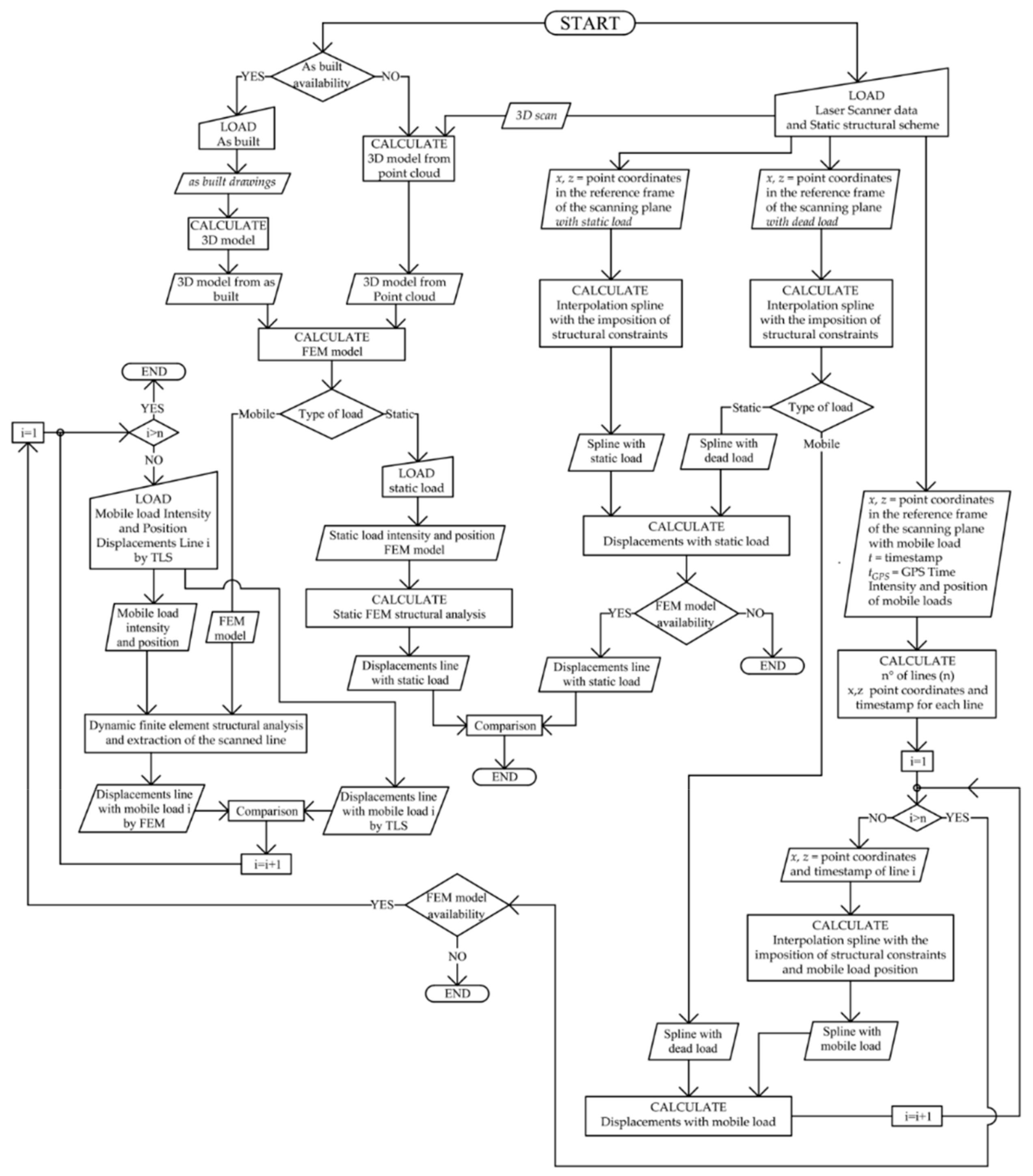
The flowchart of the implemented software is shown in Figure 2.
3. Results
3.1. The First Test: The Bridge at University of Calabria
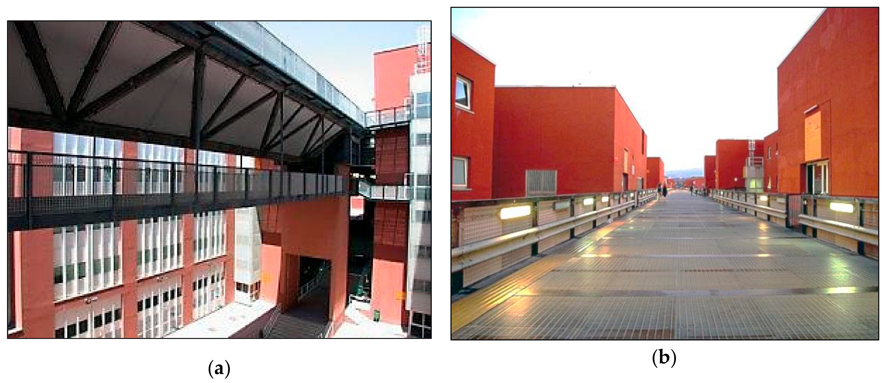
The first test was performed on a double deck bridge at the University of Calabria, Italy. The bridge materializes the South-North central axis, that characterizes the campus layout. All the buildings are lined up on the sides of the bridge. The lower deck is intended for pedestrians. The upper one is used occasionally for vehicular traffic. The main structure is a simply supported truss beam, characterized by three longitudinal tubular elements; the lower deck is hung from the upper ones (Figure 3).
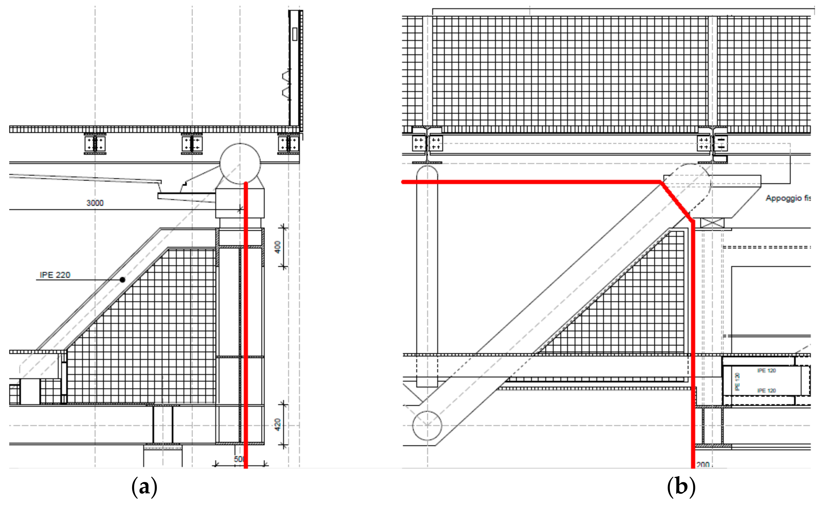
In Figure 4 the cross sections of the simply supported truss beam at the bearings are shown. The red line represents the path followed by the laser scanner during the acquisitions in line-scan mode.
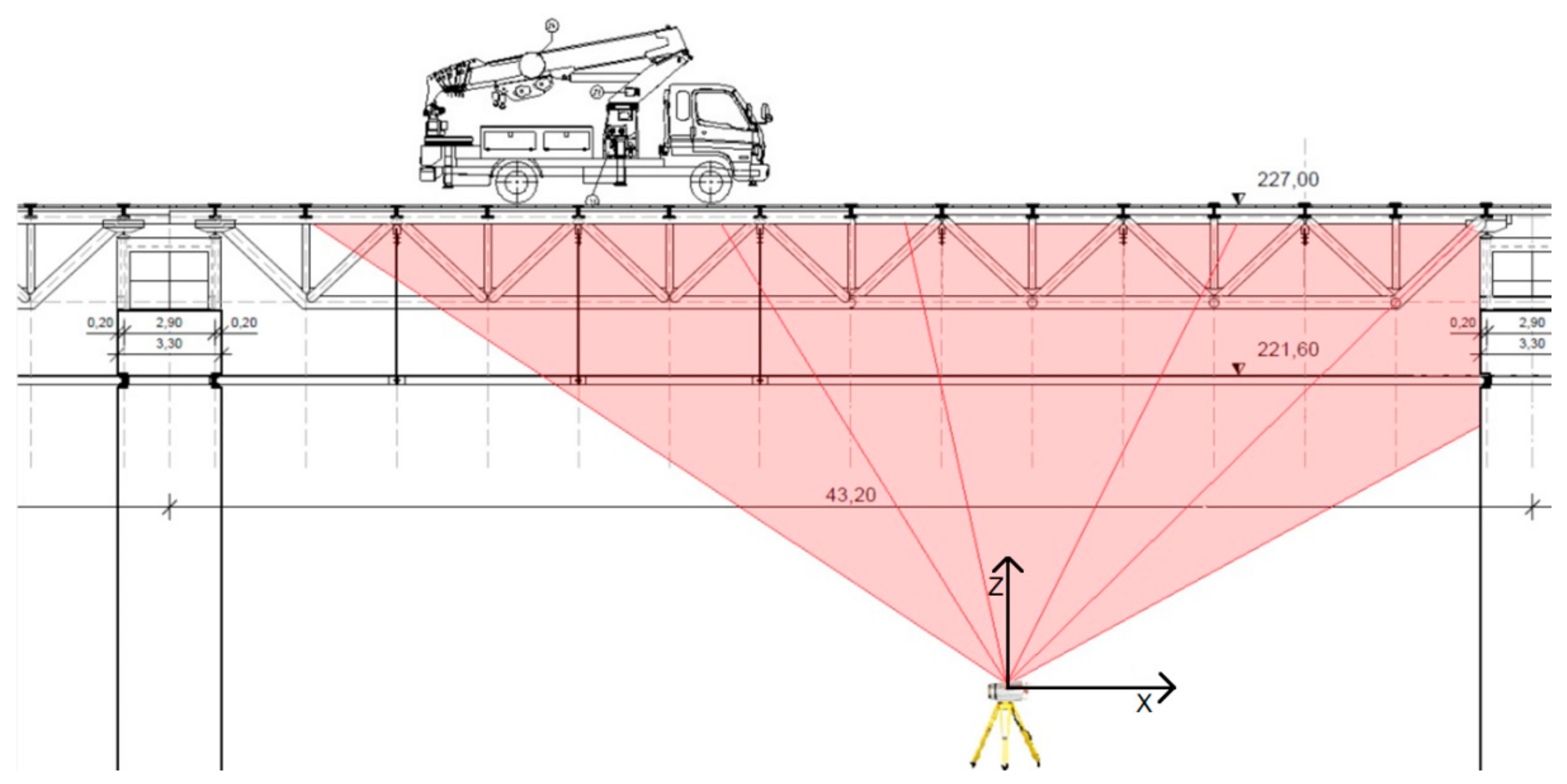
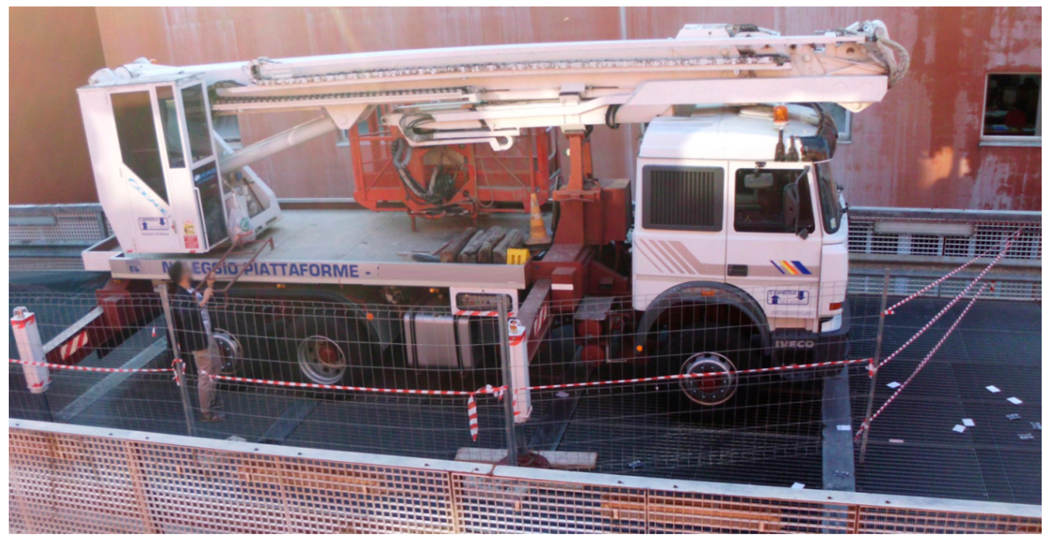
Figure 5 shows the test layout. The test was performed during the parking of a truck elevator, which weight was about 260 kN (Figure 6). The TLS position was chosen below the deck. In this way it was possible to acquire the points of the upper element of the deck structure, realized with a 3D truss. To minimize the oscillations of the rotation axis, the minimum sampling rate was chosen, equal to 70,000 points per second. The distance between the bearings of the bridge is 40.30 m. Measuring the position of the wheel axles, the center of gravity of the truck was obtained, located 11.07 m from the south support.
RiSCAN PRO®, the software provided with the TLS, was used for the first processing of data. The coordinates of the scanned points were obtained, with reference to the TLS centre and expressed in meters. The software described in Section 2.3 was then used; the following figures show the results.
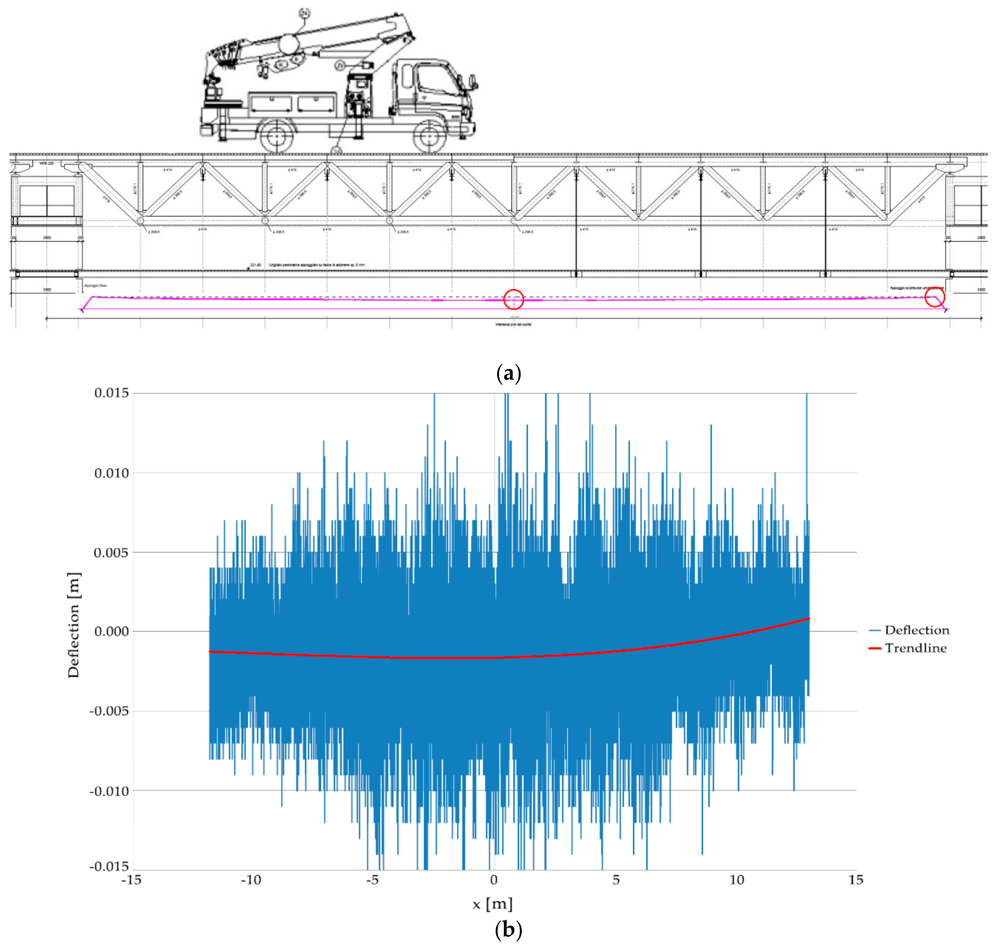
Figure 7a shows, on an arbitrary scale, a view of the entire span and of the lines obtained with the bridge loaded and without loads. The origin of the reference system is the center of TLS. One can observe that the deck has a vertical displacement, with respect to the horizontal direction, of about 134 mm in the middle of the span, with only the dead load. The circles indicate the enlargements shown in Figure 8. Figure 7b shows the deflections due to the truck load, obtained from raw data and the trend-line. In this case, a cubic polynomial, of the type described in Equations (4) and (5), provides an effective fitting line.
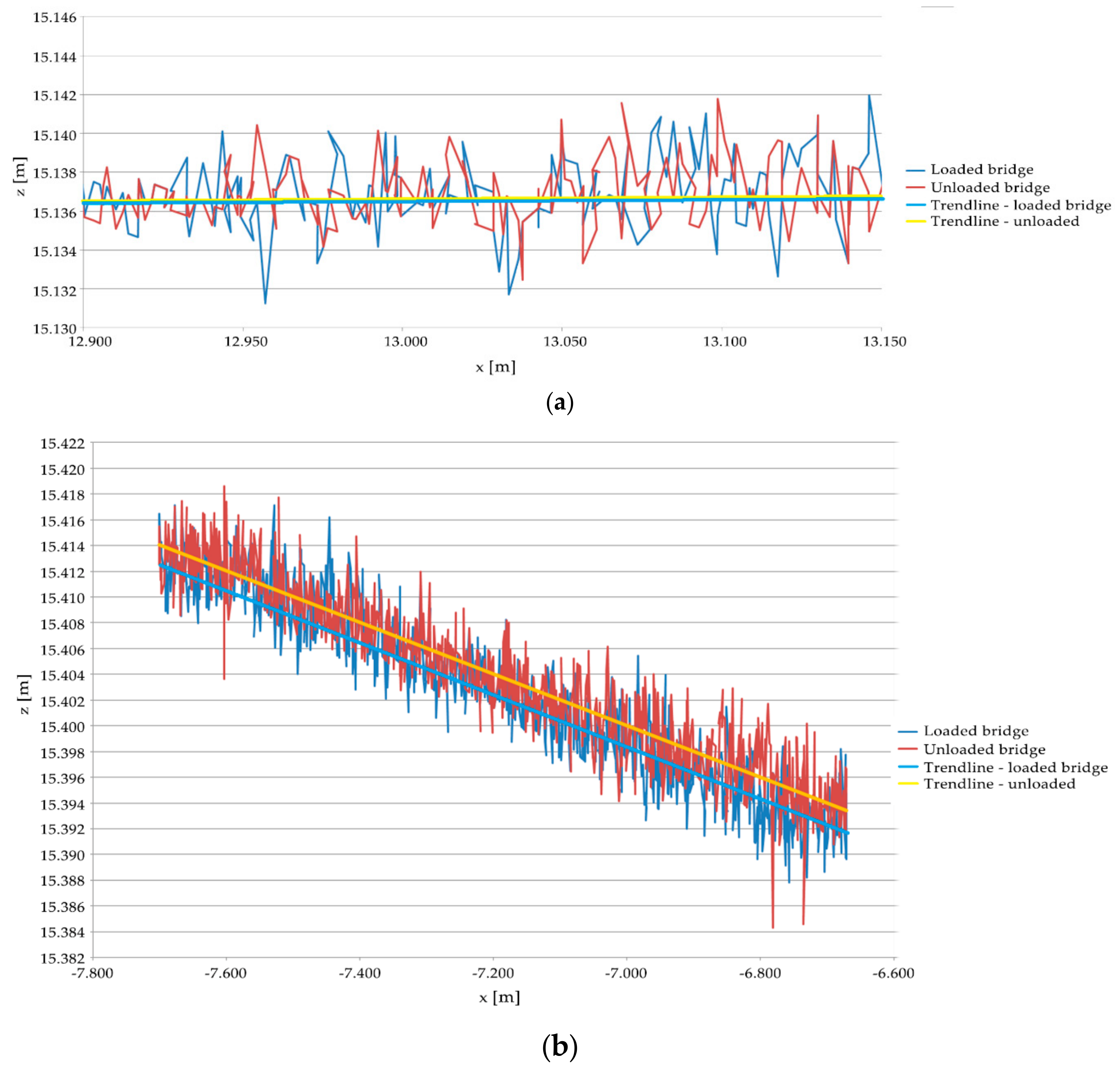
Figure 8 shows two enlargements of raw data and interpolation lines. It is possible to observe that the lines obtained with the loading and unloading bridge coincide on the bearing (Figure 8a), while in the central part of the beam there is a difference in height of about 2 mm (Figure 8b). Also in this case the coordinates are referred to the intrinsic reference system of the instrument.
Using a FEM program developed at the University of Calabria [31], it was obtained an accurate evaluation of vertical displacements. The computed deflection was 1.95 mm, 2.5% less than the value attained by using the proposed methodology. Furthermore, by means of a total station Leica 1201+, a precise measurement was performed. A prism was placed in the middle of the span and was repeatedly monitored from a distance of about 22 m. The automatic target recognition function (ATR) has been activated, which has an accuracy of 1 s; therefore the vertical displacements are obtained with an accuracy of about 0.1 mm. The variation of the bridge deflection thus obtained was 1.9 mm, 5% less than that obtained using the proposed methodology.
3.2. The Second Test: The Cannavino Bridge at Celico
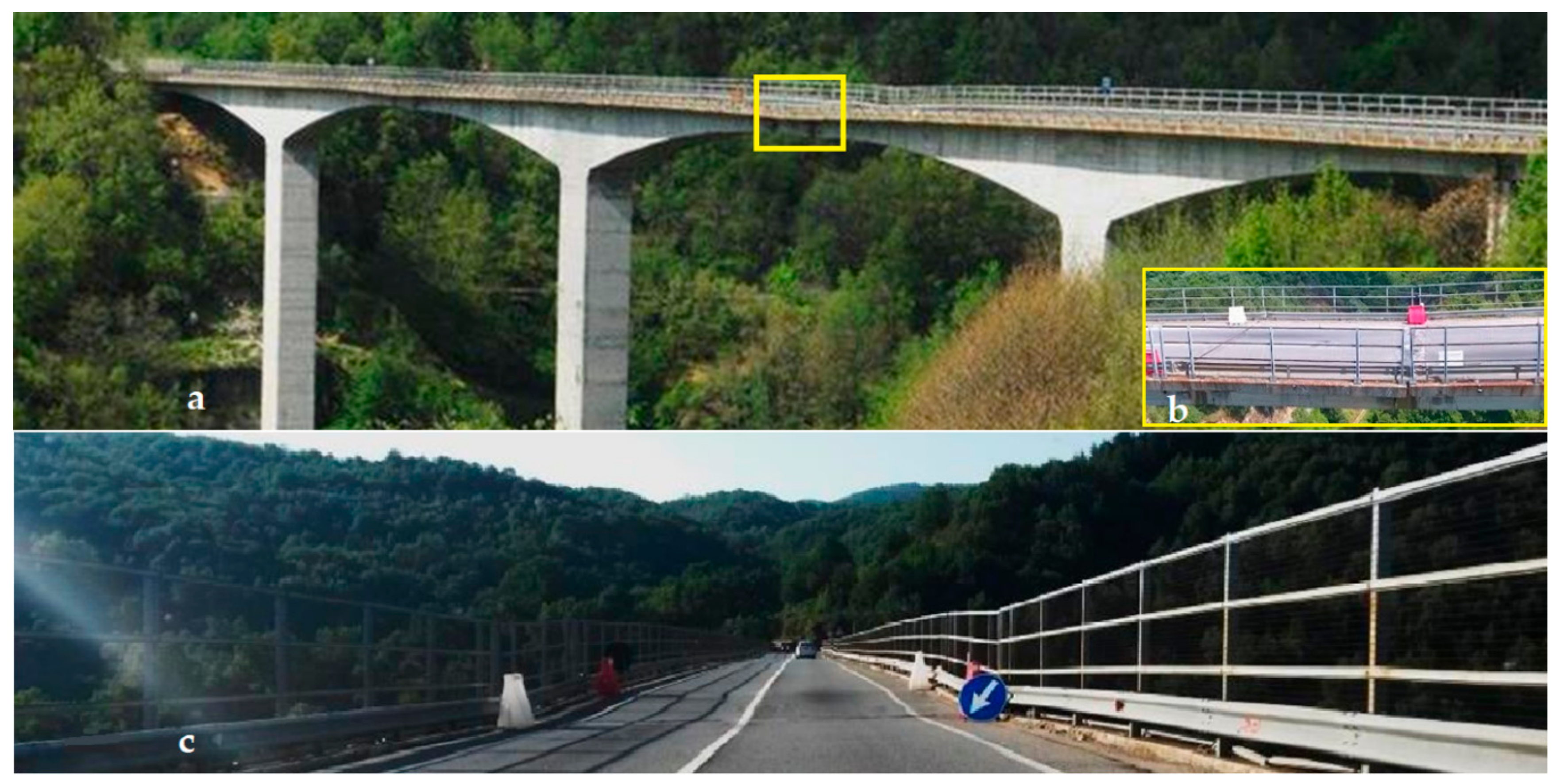
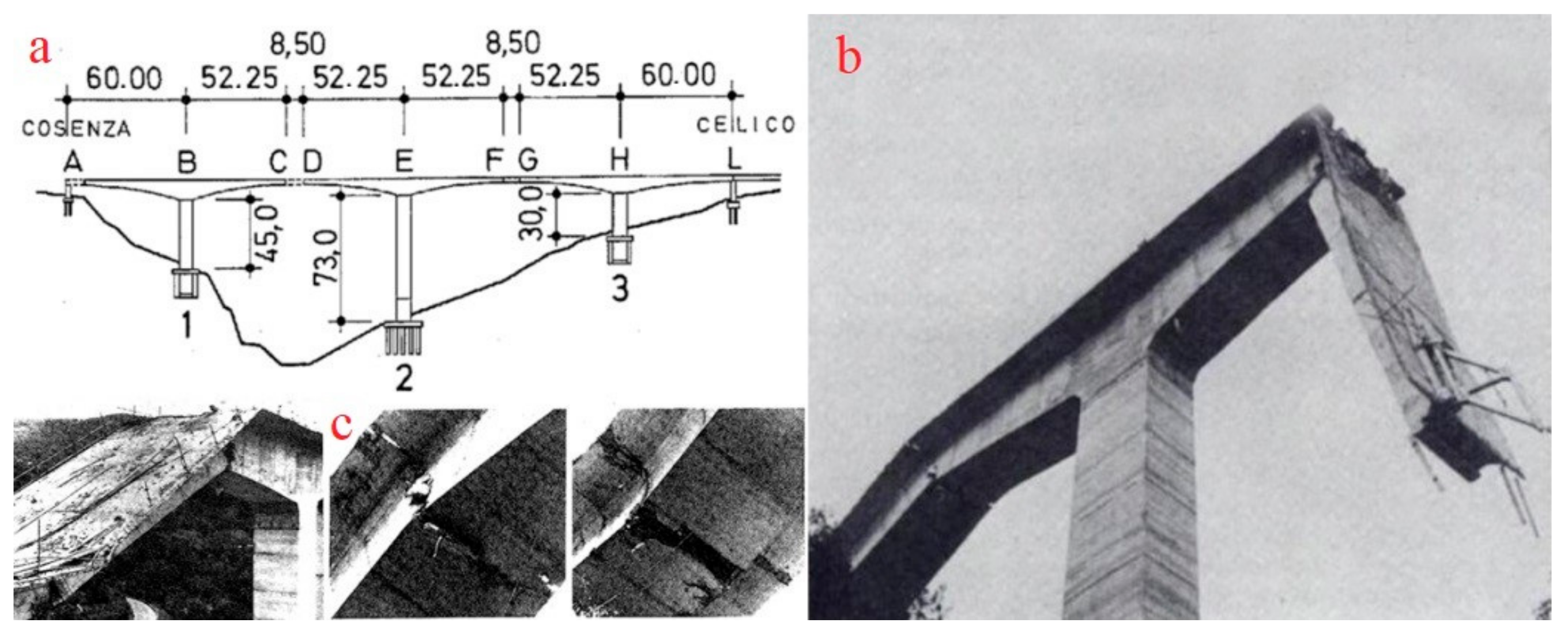
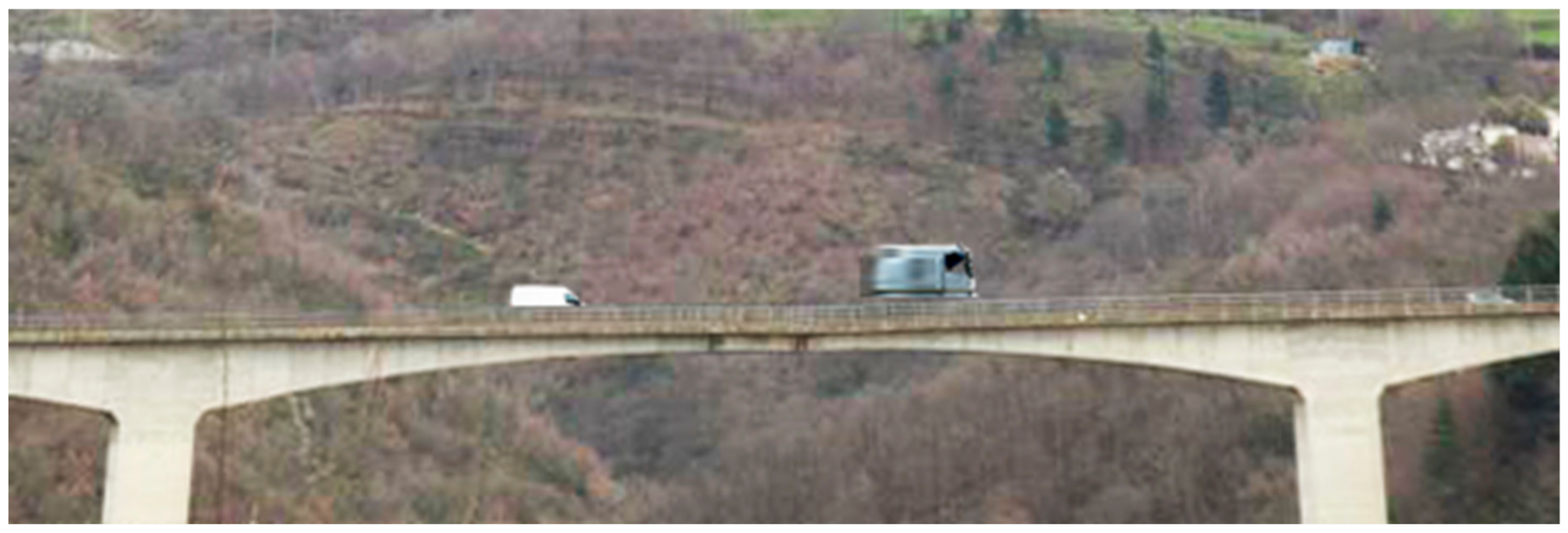
The Cannavino bridge (Figure 9a) has been realized of prestressed concrete. The structural scheme makes use of opposing cantilevers, whose ends recently have been subjected to large deflections (Figure 9 ); for this reason the technicians of ANAS, the Italian National Autonomous Roads Corporation, carry out periodic monitoring with the total station [32].
In 1972, during its construction, the bridge suffered the collapse of two cantilevers. To understand the reasons, some in-depth studies were carried out [33].
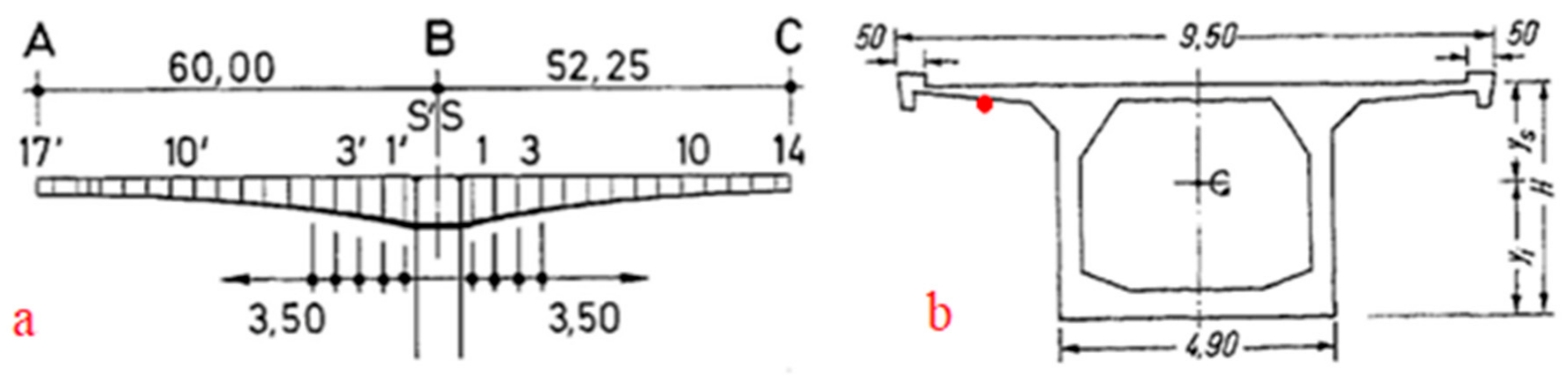
In Figure 10, one can see the elevation of the bridge (Figure 10a), a photo of the collapsed cantilevers (Figure 10b) and some details at the breaking points (Figure 10c). Figure 11 shows the south side balanced cantilever with the post-tensioned segments (Figure 11a) and their cross section (Figure 11b); the red dot indicates the line scanned during the test. The height of the segments ranges from 2.00 to 7.80 m. Figure 10 and Figure 11 are taken from [33].
The above described VZ1000 TLS was used, set up as a line scanner. To record the sampling time of each acquired point, the timestamp function has been activated. GPS time was acquired using the receiver of which TLS is provided.
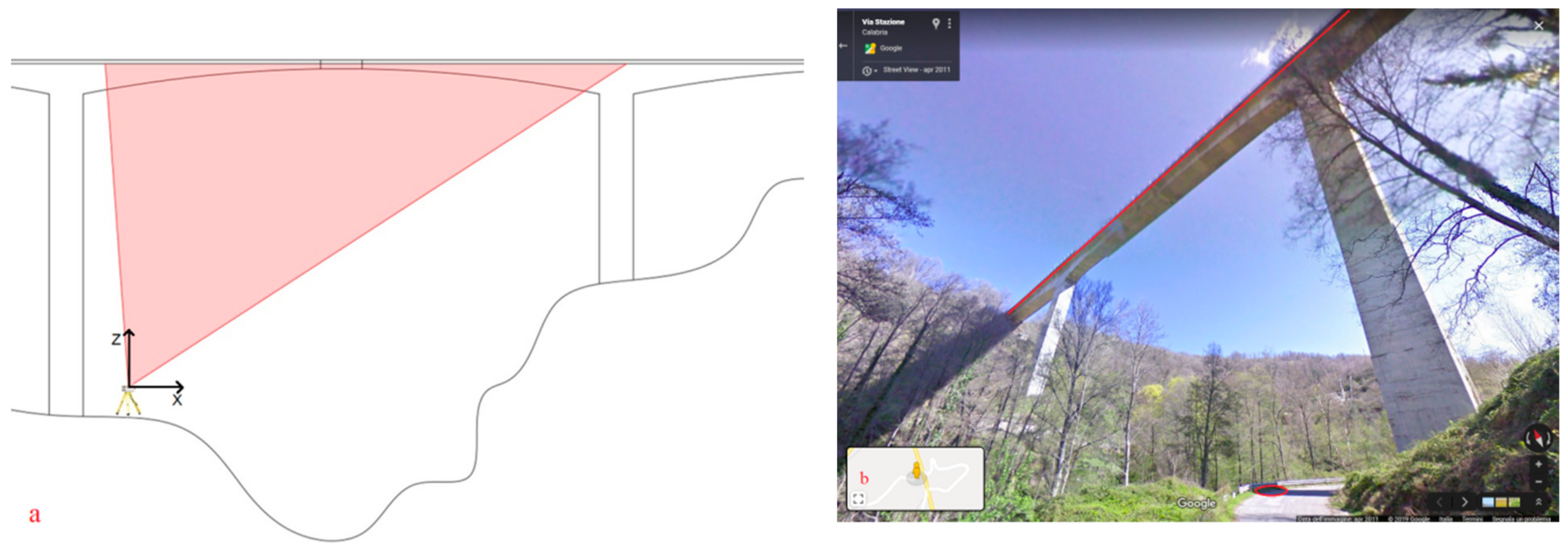
Figure 12a shows the layout of the test. The TLS station point was chosen under a cantilever, close to a pile. A path parallel to the longitudinal axis of the bridge, at the bottom of the sidewalk, was acquired for 60 s, in order to avoid an excessive size of the file to be processed (Figure 12b). The scans were carried out with the bridge open to traffic. It was chosen a 110,000 points per second scanning speed.
RiSCAN PRO® software was used to process the acquired data. Point coordinates and timestamps have been recorded in a text file. Subsequently the file was processed with the previously described Matlab® code and the single lines were extracted and corrected, by imposing the structural constraints. The splines were then calculated for each scanned line.
The video of the loads was acquired with the above described digital camera, equipped with a GP-1 unit, an accessory capable of providing Coordinated Universal Time (UTC) (Figure 13).
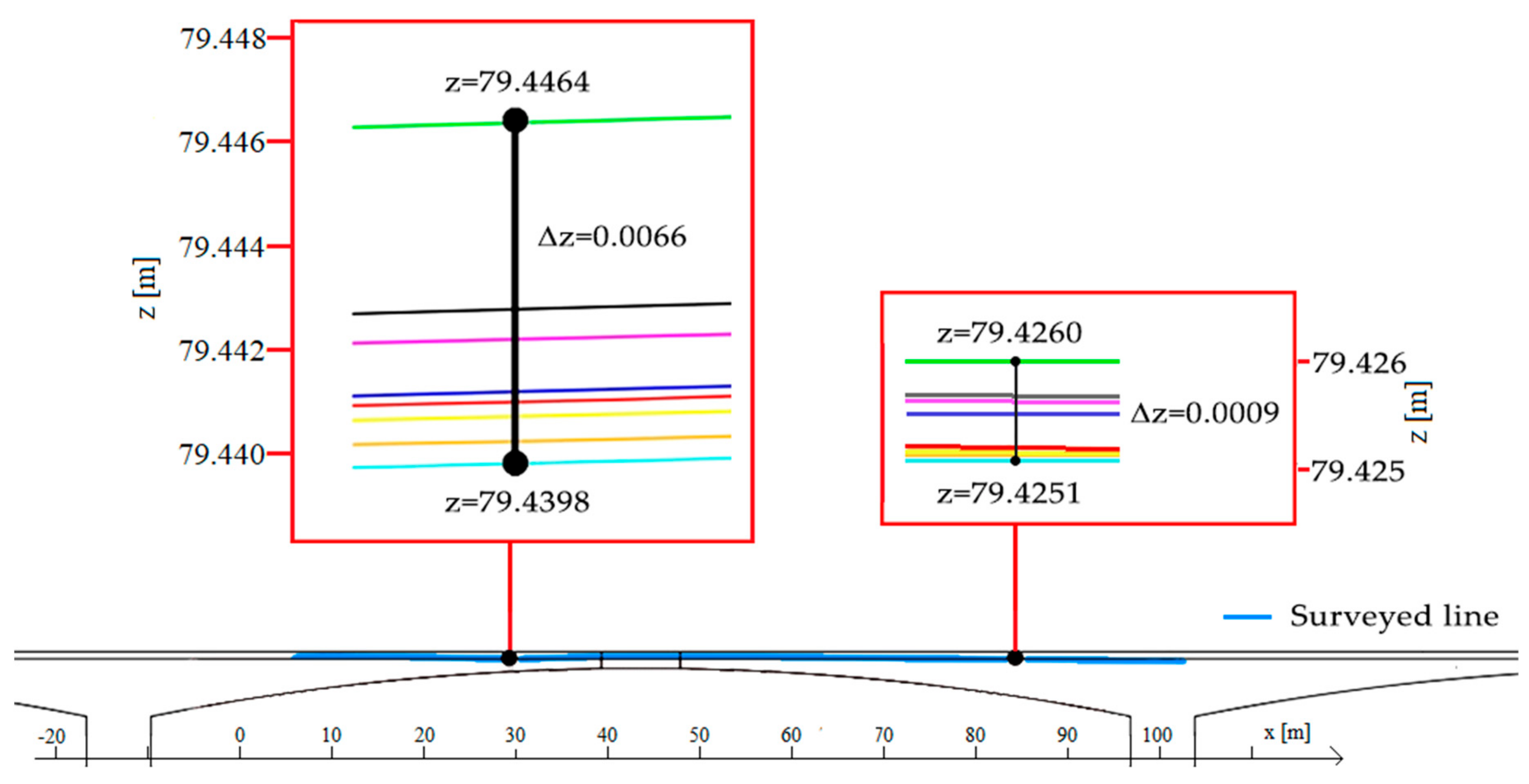
Figure 14 shows a stretch of the splines obtained for six load combinations; the reference system of the TLS shown in Figure 12 was used for the coordinates in meters.
The green line is obtained for the maximum load visible in the frame of Figure 13. The cyan line refers to the unloading bridge, while the other lines refer to intermediate load conditions. As regards the position of the loads, they were obtained approximately taking into account the posts of the guardrails. Loads were estimated based on the type of vehicles present in each selected frame. A FEM analysis was performed using the aforementioned code [31], the structural data provided by [33] and the six load combinations.
The following remarks can be made: (a) towards the free end of the cantilever, the splines diverge (different colors correspond to different times) when the mobile loads increase; (b) the maximum distance is about 6 mm; (c) The FEM analysis provides 16% lower results, with a maximum displacement of 5 mm. This difference is understandable given the uncertainty in the evaluation of loads, the unavailability of the as built and the age of the structure. A comparison was made with the outcomes of the load tests carried out by the technicians of ANAS some years earlier with higher loads. The results obtained, taking into account the ratio between the loads in the two tests, show a difference of about 10%
3.3. The Third Test: The Santiago Calatrava’s San Francesco Bridge at Cosenza
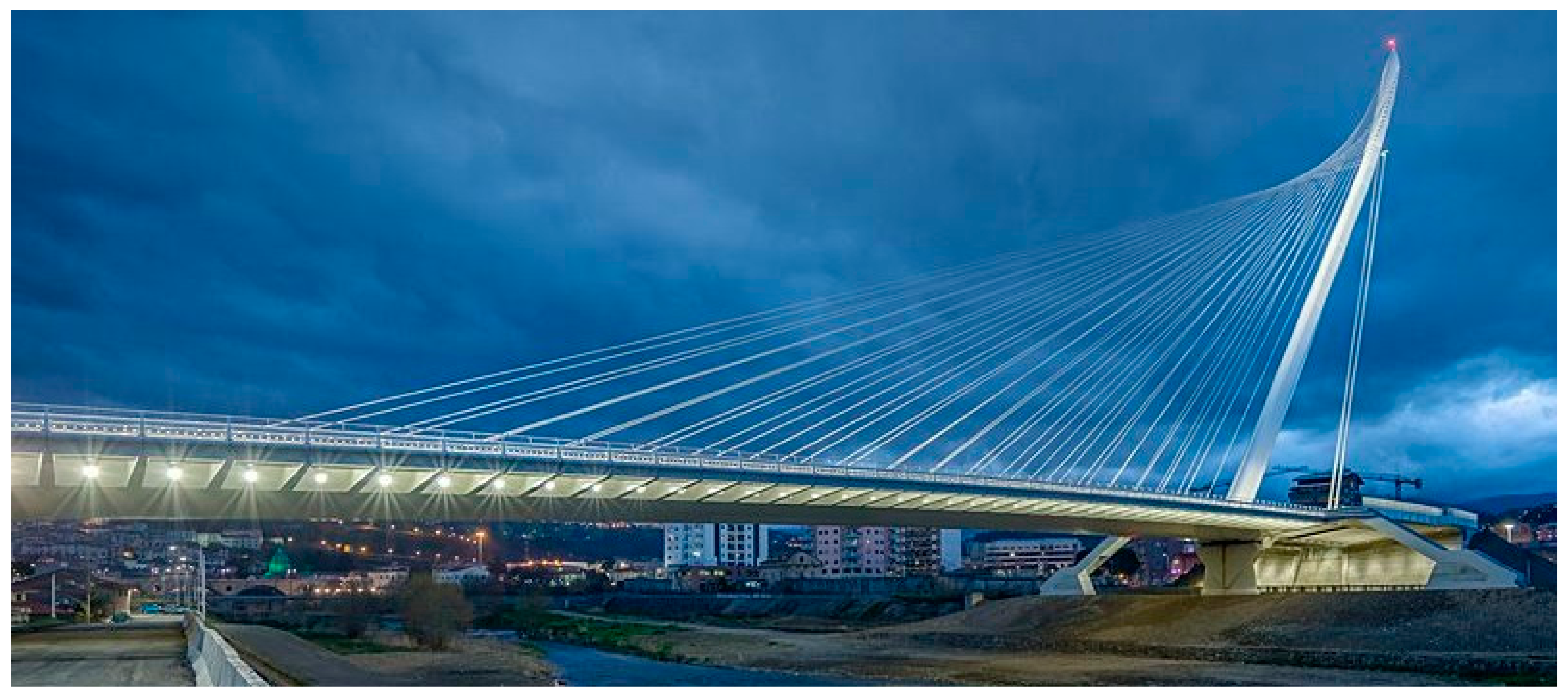
Built to allow an access large and of artistic value to the city of Cosenza, the large structure of San Francesco Bridge (Figure 15) crosses the Crati river.
It is a cable-stayed bridge with a cantilever spar. The characterizing structural element is the single inclined pylon, which with its height of 95 m marks the surrounding landscape. The span, 200 m long, is counterbalanced by twenty twin cable lengths. Two large rods contrast the actions of the cables. A special feature of the bridge is the upper part of the pylon, where the cables are anchored so as to give the impression of a sail. The metal structure of the deck rests on artistically sculpted concrete abutments.
To represent work and the surrounding area of the city, a survey was conducted using a TLS [34]. The surveyed area extends to the historic center and covers the riverbed. (Figure 16).
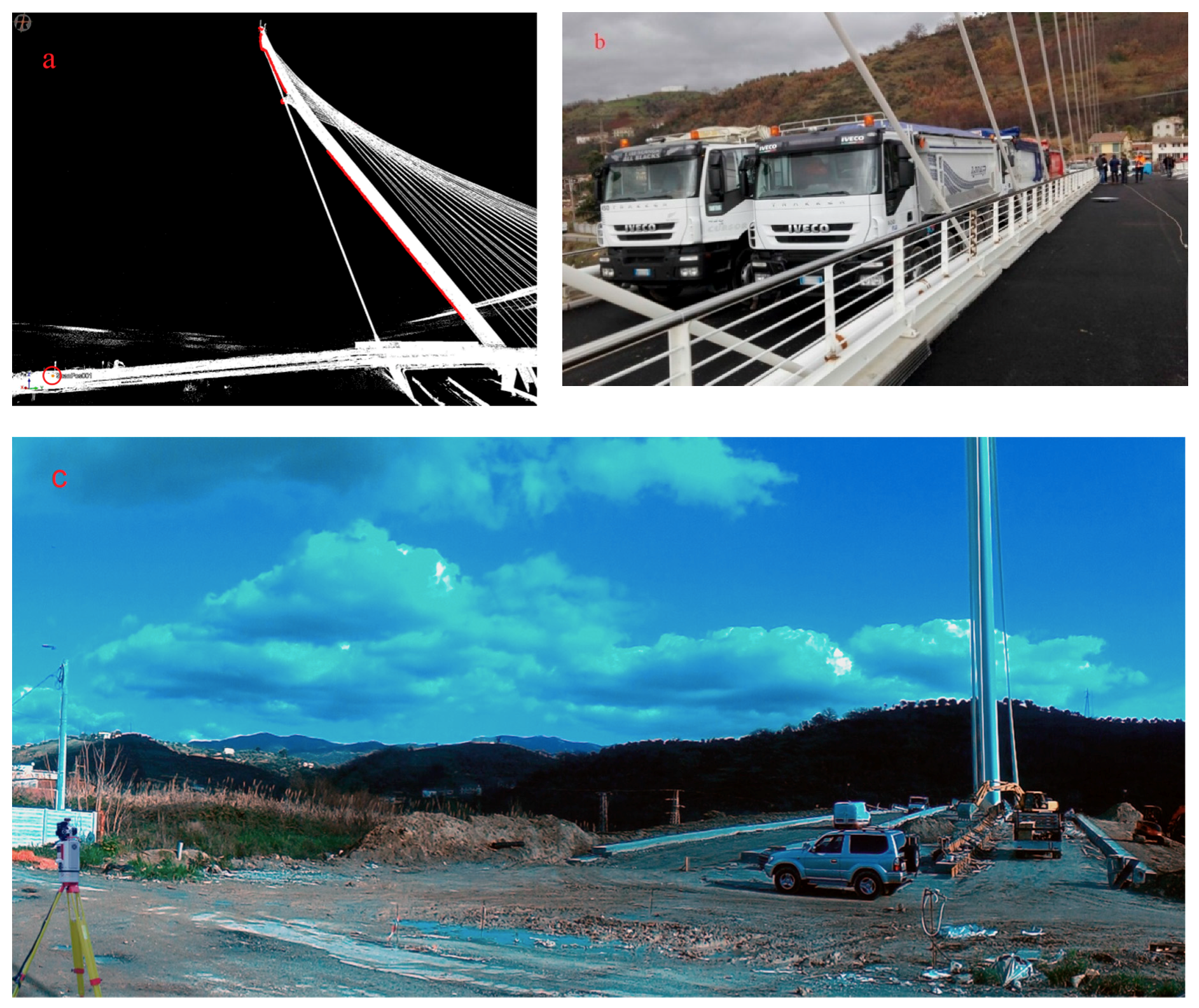
The experiment was performed during the official load test carried out on 17 January 2018, a windy day; a series of trucks of known weight were placed on the deck (Figure 17b).
Several instruments were used during the test. In addition to a digital level and a total station; some strain sensors were placed both on the pylon and in various positions on the deck. Furthermore, two inclination sensors provided inclination at different pylon heights in real time, thanks to a wireless connection [35].
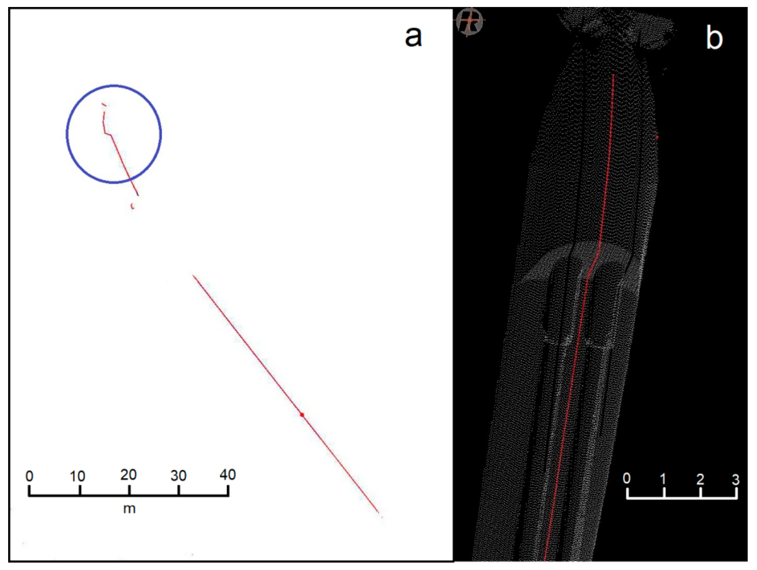
A station point for VZ1000 TLS was chosen, aligned with the central axis of the bridge. The chosen location is in a stable area and is about 90 m from the anchorage of the rods. This position allows a vertical section of the pylon to be described with the laser beam of the instrument. In particular, the outer part of its cylindrical surface with elliptical section is detected. The rods hidden only a short stretch of the pylon. In this way, we can get the elastic line of the pylon for each line scan, during the runs of the trucks used as mobile loads.
Figure 17a shows the layout of the test. On the left side of the panel, you can see the TLS station. The laser trace is highlighted by a red line. Figure 18a shows a vertical section extracted from a line scan. Figure 18b shows the point cloud obtained for the pylon head. Overlaid you can see the upper part of the laser track, circled in blue in Figure 18a.
The official load test involved the sequential positioning of ten trucks side by side on two adjacent lanes (Figure 17b). The TLS acquisitions were made in two configurations: (a) with unloaded bridge, (b) during the load test.
The unloaded bridge acquisition was carried out from 11.33 am to 11.35 am local time (UTC + 1). The acquisition with mobile loads was carried out from 10:41 UTC (GPS time 1,200,220,888) to 10.51 UTC (GPS time 1,200,221,500). The sampling rate was 120 lines per second. This acquisition began before the first truck left and continued until before the departure of the fourth truck. The scans were then stopped due to the heavy rain, so the runs of the last vehicles were not acquired. The trucks were equipped with Leica GS15 GNSS receivers, mounted on a solid magnetic base that allows them to be fixed to the cab roof.
The recording rate was set to 5 Hz. The data collected by the permanent GNSS station of the University of Calabria were used to perform post processing.
Table 4 shows the GPS time for the actions performed during the load test.
A comparison between the results obtained by the total station and the acquisitions of the TLS in line scanner mode showed a substantial agreement between the two techniques. Also the comparison with the acquisitions of inclination sensors confirmed the reliability of the methodology.
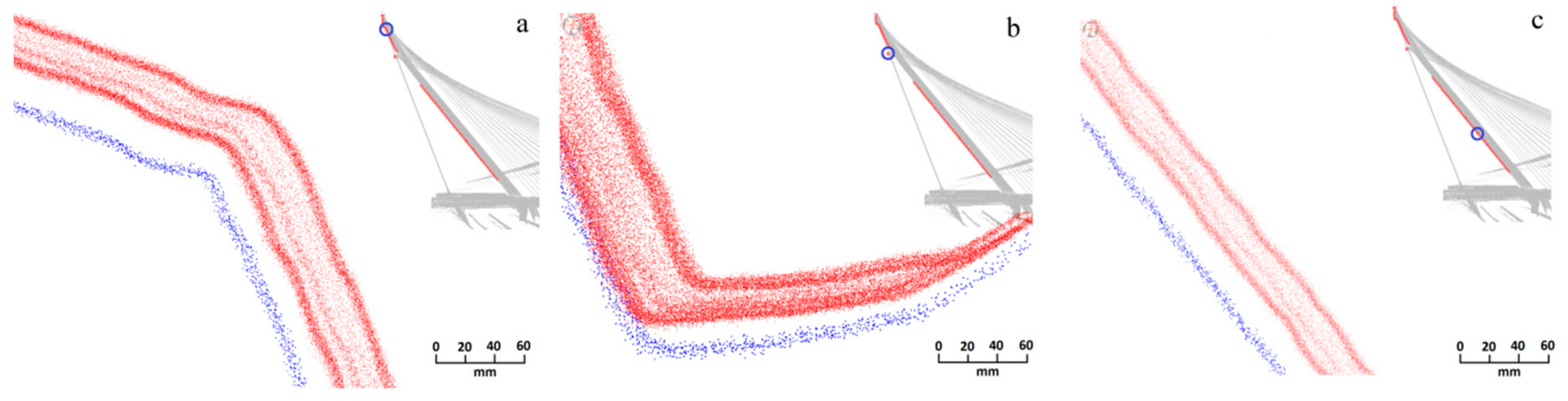
Figure 19 shows some test results. The magnifications correspond to the areas circled in blue in the thumbnails. The point cloud of the profile acquired with the unloaded bridge is in blue.
First of all we can see that the precision declared for the instrument and reported in Table 1 is confirmed. The cloud of blue points, in fact, is about 8 mm thick. Therefore the precision of the acquisitions is about ten times lower than the displacements we have to measure.
In the panel 19a we can see the displacements of the pylon head. The height, referred to the TLS centre, is about 81 m. The dense red point cloud on the left was obtained during the stop of the first truck. The red dense point clouds on the right were obtained during the short stop of the second truck and during the stop of the third one. At the end of the TLS acquisitions, three trucks were positioned on the bridge. Also this point cloud is 8 mm thick. Scattered points were acquired while the second and third trucks were running. Point clouds acquired during truck slowdown become denser. We observe an overall displacement of 41 mm. The first two mobile loads caused roughly half of the total displacement.
In the panel 19b one can see the points acquired in correspondence with the constraint device in which the rods can slide, 69 m above the TLS. In this case, we can see that the horizontal displacements begin with the run of the second truck. The analysis of this behavior is outside the scope of our study. The maximum displacements are slightly lower with respect to the upper part. Since these zones are close together, this behavior seems reasonable.
The points acquired in the lowest part of the pylon are shown in panel 19c. The height of this zone is 39 m respect to the TLS center. The displacements reach a maximum value of 26 mm.
Using the Matlab code described above, the individual lines from the overall file supplied by the TLS were extracted and a timestamp was associated to each line. The interpolating lines were then determined.
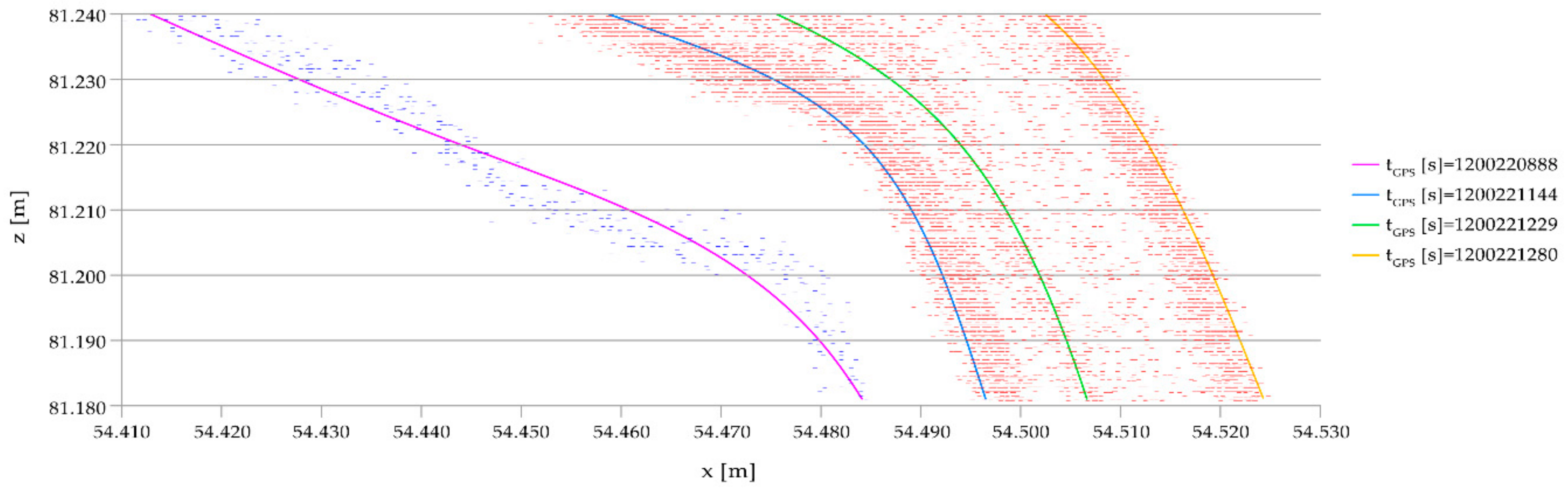
Figure 20 shows a stretch of four splines, obtained for different instants, in the upper zone of the pylon. The coordinates are referred to the center of the instrument, so x is the horizontal distance and z is the difference in height with respect to the center of the TLS. The magenta line (GPS TIME 1200220928) is related to the unloading bridge. The other lines relate to the parking of the first truck (blue line), the parking of the second truck alongside the first one (green line) and the parking of the first three trucks (yellow line). From the data collected it is possible to extract the movements of the pylon, at each height, as a function of time.
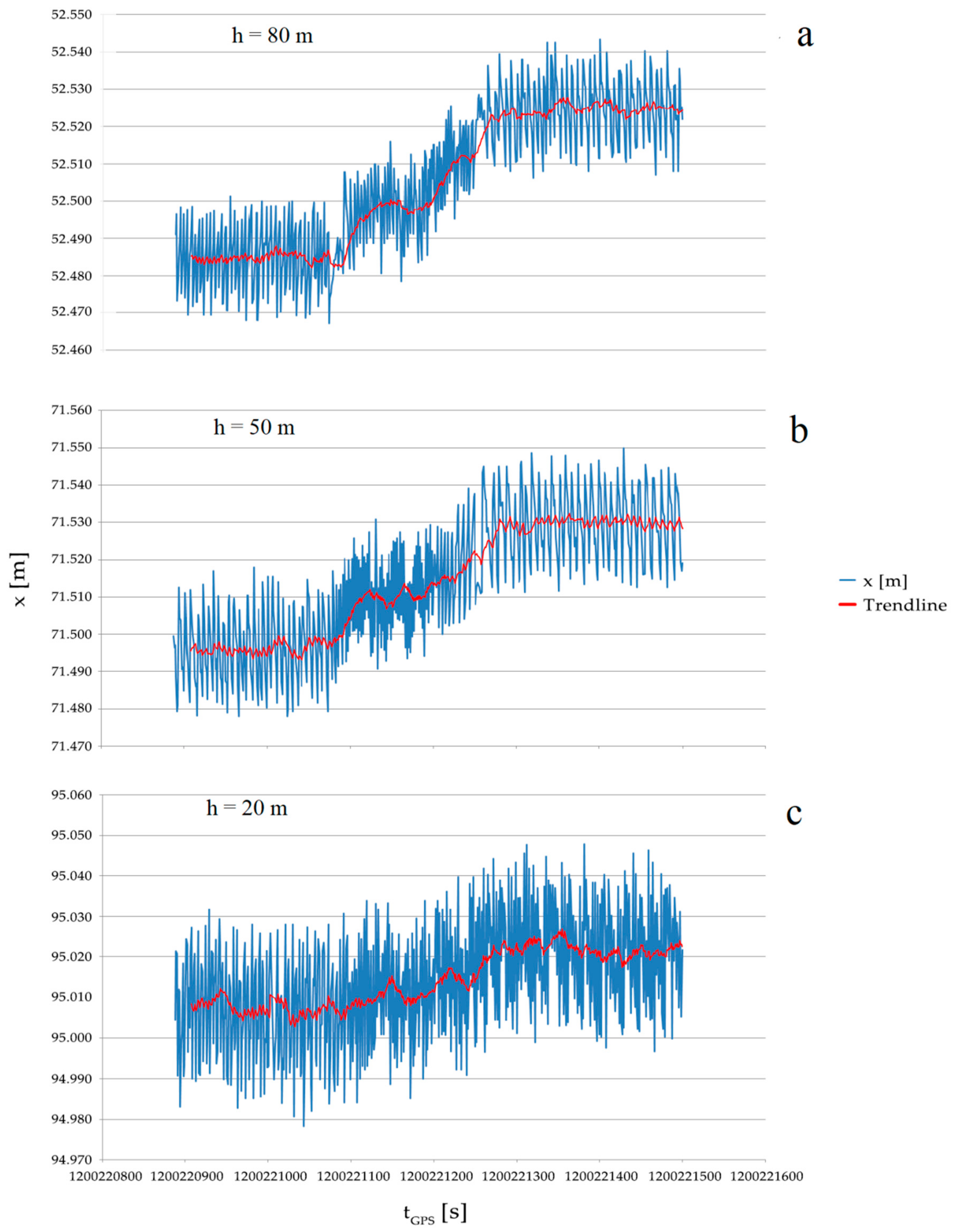
Figure 21 shows the horizontal movements of the pylon at three different heights. In panel (a) we observe the movements of a point at a height of 80 m with respect to the instrument, as a function of the GPS time. The displacements due to the moving loads are easily recognizable by analyzing the 10 samples moving average, drawn in red: during the run of the first truck the point moves up to 15 mm towards the midspan. The point does not move during the stop and undergoes a further displacement during the run of the second truck. After a brief pause, the third movement begins, ending with the halt of the third truck. The total displacement is about 41 mm. It is worth remarking that the graph reflects the times of the events reported in Table 4.
The comments made above can be repeated for the point at a height of 50 m, which movements are drawn in the panel (b). Displacements are reduced, as expected.
As regards the point at 20 m height, the various phases are less evident. A final displacement of about 16 mm can be observed.
Measurements were performed with a total station after positioning each of the three trucks. The station pointed targets placed on the pylon at various heights and its measurements were used for the official load test. The results fully agree with those obtained with our method. Also the inclination variations sampled by two sensors, positioned inside the pylon and connected wirelessly, are consistent with the splines extracted using the method described.
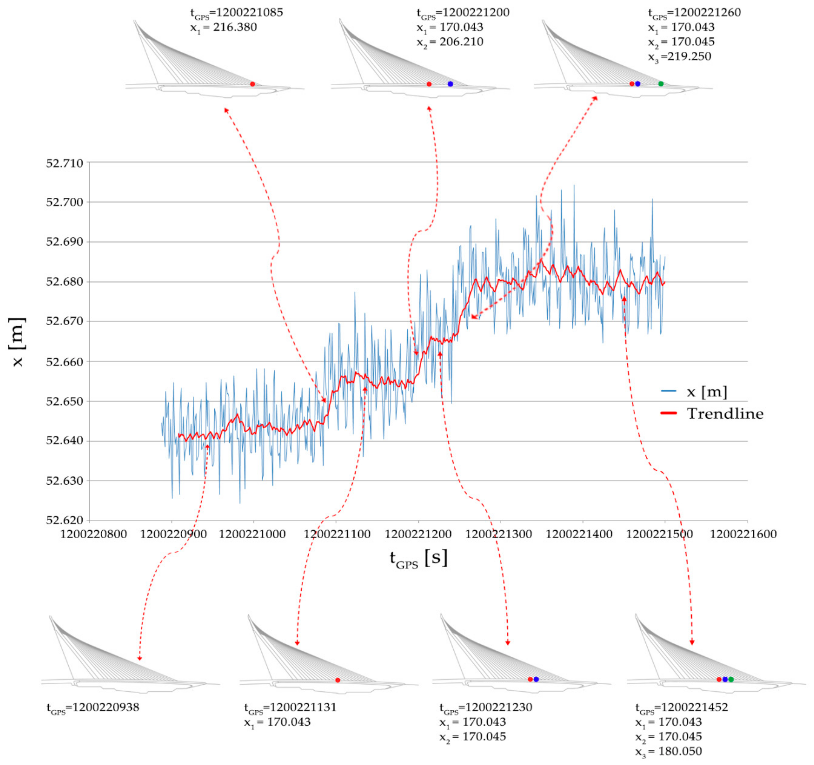
Thanks to the acquisitions made by the GNSS receivers positioned on the trucks, the displacements of the points of the pylon can finally be correlated to the position of the mobile loads. Since the TLS position was obtained thanks to its GPS receiver, the coordinates of the each mobile vehicle, for each GPS time, can be converted into local coordinates in the TLS reference frame.
The correlation is shown in Figure 22 in which the horizontal positions of a point of the upper part of pylon are represented as a function of GPS time. The point is 85 m above the TLS centre. The trend-line evidences runs and stops of the trucks. In the thumbnails, the GPS time and the instantaneous local coordinate x of the moving loads, represented by dots, are shown. The red, blue and green dots represent, respectively, the first, second and third trucks.
4. Discussion
The three tests carried out allows us to make the following remarks.
The reliability of the method, if complete information on the materials and on the structural scheme is available, has been demonstrated with the first test. The displacements obtained under static loading conditions, approximated using a cubic polynomial, differ by approximately 2.5% from those obtained from the FEM analysis and by about 5% from the results provided by independent precise measurements.
The applicability of the method to structures more complex and with less information was verified with the second test, carried out on a bridge characterized by relaxation and creep phenomena, in normal traffic conditions. The difference between the results obtained with the method described and those of a FEM analysis is about 16%. Compared to the outcomes of the aforementioned measurements carried out by the technicians of ANAS, the difference decreases to about 10%. In any case, the results obtained are acceptable for an estimate of the behavior of the structures.
As regards the third test, the comparison with the results obtained with other techniques and instrumentations (total station and inclination sensors) confirmed the validity and precision of the methodology.
In all the tests, the use of interpolating lines allowed to get higher precision with respect to the unmodeled observations. The working hypotheses, therefore, proved to be reliable.
A peculiarity of the technique described is the possibility of obtaining the 3D model of the monitored structure and the dynamic linear survey with the same instrument and reference system (Figure 18).
Possible fields of application of the methodology presented are both road and railway infrastructures, tall structures and buildings. The method proves particularly valid for constructions characterized by remarkable spans and/or great heights.
A limit to its usability is given by the need to have a point to position the TLS, with a clear view of the whole or at least of most of the structure to be monitored.
The integration with different techniques opens up the prospect of interesting uses. In the immediate future, activities are planned to exploit the high acquisition rate of TLS, in order to determine the natural frequencies of structures. To this end, acquisitions will be performed simultaneously using TLS and Ground Based Radar Interferometry.
Author Contributions
Conceptualization, S.A.; methodology, S.A.; software S.A.; validation, S.A. and R.Z.; structural investigation, R.Z.; resources, R.Z.; data curation, S.A.; writing—original draft preparation, S.A.; writing—review and editing, S.A. and R.Z.; visualization, S.A. All authors have read and agreed to the published version of the manuscript.
Funding
This research received no external funding.
Conflicts of Interest
The authors declare no conflict of interest.
References
- Lantsoght, E.O.L.; der Veen, C.; Boer, A.; Hordijk, D.A. State-of-the-art on load testing of concrete bridges. Eng. Struct. 2017, 150, 2312–2341. [Google Scholar] [CrossRef] [Green Version]
- Zinno, R.; Artese, S.; Clausi, G.; Magarò, F.; Meduri, S.; Miceli, A.; Venneri, A. Structural Health Monitoring (SHM). In The Internet of Things for Smart Urban Ecosystems; Cicirelli, F., Guerrieri, A., Mastroianni, C., Spezzano, G., Vinci, A., Eds.; Springer International Publishing: Switzerland, Cham, 2019; pp. 225–249. [Google Scholar] [CrossRef]
- Fan, W.; Qiao, P. Vibration-based damage identification methods: A review and comparative study. Struct. Health Monit. 2011, 10, 83–111. [Google Scholar] [CrossRef]
- Malekjafarian, A.; McGetrick, P.J.; OBrien, E.J. A Review of Indirect Bridge Monitoring Using Passing Vehicles. Shock Vib. 2015, 2015, 286139. [Google Scholar] [CrossRef] [Green Version]
- Carpinteri, A.; Lacidogna, G.; Pugno, N. Structural damage diagnosis and life-time assessment by Acoustic Emission monitoring. Eng. Fract. Mech. 2007, 74, 273–289. [Google Scholar] [CrossRef]
- Davis, A.; Mirsayar, M.; Hartl, D. Structural health monitoring using embedded magnetic shape memory alloys for magnetic sensing. In Proceedings of the SPIE–International Society for Optics and Photonics, Nondestructive Characterization and Monitoring of Advanced Materials, Aerospace, Civil Infrastructure, and Transportation XIII, Bellingham, WA, USA, 4–7 March 2019; Gyekenyesi, A.L., Ed.; Volume 10971. [Google Scholar]
- Morris, I.; Abdel-Jaber, H.; Glisic, B. Quantitative Attribute Analyses with Ground Penetrating Radar for Infrastructure Assessments and Structural Health Monitoring. Sensors 2019, 19, 1637. [Google Scholar] [CrossRef] [Green Version]
- Artese, S.; Perrelli, M. Monitoring a Landslide with High Accuracy by Total Station: A DTM-Based Model to Correct for the Atmospheric Effects. Geosciences 2018, 8, 46. [Google Scholar] [CrossRef] [Green Version]
- Artese, G.; Perrelli, M.; Artese, S.; Manieri, F. Geomatics activities for monitoring the large landslide of Maierato, Italy. Appl. Geomat. 2015, 7, 171. [Google Scholar] [CrossRef]
- Lienhart, W.; Ehrhart, M.; Grick, M. High Frequent Total Station Measurements for the Monitoring of Bridge Vibrations. In Proceedings of the 3rd Joint International Symposium on Deformation Monitoring (JISDM), Vienna, Austria, 30 March–1 April 2016; Available online: https://www.fig.net/resources/proceedings/2016/ (accessed on 2 September 2019).
- Yu, J.; Zhu, P.; Xu, B.; Meng, X. Experimental assessment of high sampling-rate robotic total station for monitoring bridge dynamic responses. Measurement 2017, 104, 60–69. [Google Scholar] [CrossRef]
- Lovse, J.W.; Teskey, W.F.; Lachapelle, G.; Cannon, M.E. 7-Dynamic Deformation Monitoring of Tall Structure Using GPS Technology. J. Surv. Eng. 1995, 121, 35–40. [Google Scholar] [CrossRef]
- Roberts, G.W.; Meng, X.; Dodson, A.H. Integrating a global positioning system and accelerometers to monitor the deflection of bridges. J. Surv. Eng. 2004, 130, 65–72. [Google Scholar] [CrossRef]
- Yu, J.; Meng, X.; Shao, X.; Yan, B.; Yang, L. Identification of dynamic displacements and modal frequencies of a medium-span suspension bridge using multimode GNSS processing. Eng. Struct. 2014, 81, 432–443. [Google Scholar] [CrossRef]
- Jo, B.W.; Lee, Y.S.; Jo, J.H.; Khan, R.M.A. Computer Vision-Based Bridge Displacement Measurements Using Rotation-Invariant Image Processing Technique. Sustainability 2018, 10, 1785. [Google Scholar] [CrossRef] [Green Version]
- Baohua Shan, B.; Wang, L.; Huo, X.; Yuan, W.; Xue, Z. A Bridge Deflection Monitoring System Based on CCD. Adv. Mater. Sci. Eng. 2016, 2016, 4857373. [Google Scholar] [CrossRef] [Green Version]
- Xu, Y.; Brownjohn, J.M.W. Review of machine-vision based methodologies for displacement measurement in civil structures. J. Civil Struct. Health Monit. 2018, 8, 91. [Google Scholar] [CrossRef] [Green Version]
- Feng, D.; Feng, M.Q. Experimental validation of cost-effective vision-based structural health monitoring. Mech. Syst. Signal Process. 2017, 88, 199–211. [Google Scholar] [CrossRef]
- Yoneyama, S.; Ueda, H. Bridge Deflection Measurement Using Digital Image Correlation with Camera Movement Correction. Mater. Trans. 2012, 53, 285–290. [Google Scholar] [CrossRef] [Green Version]
- Pepe, M. Image-based methods for metric surveys of buildings using modern optical sensors and tools: From 2D approach to 3D and vice versa. Int. J. Civil Eng. Technol. 2018, 9, 729–745. [Google Scholar]
- Yan, Y.; Hang, L.; Dongsheng, L.; Xingquan, M.; Jinping, O. Bridge Deflection Measurement Using Wireless MEMS Inclination Sensor Systems. Int. J. Smart Sens. Intell. Syst. 2013, 6, 38–57. [Google Scholar] [CrossRef] [Green Version]
- Zhao, X.; Liu, H.; Yu, Y.; Xu, X.; Hu, W.; Li, M.; Ou, J. Bridge displacement monitoring method based on laser projection-sensing technology. Sensors 2015, 15, 8444–8463. [Google Scholar] [CrossRef]
- Artese, S.; Achilli, V.; Zinno, R. Monitoring of Bridges by a Laser Pointer: Dynamic Measurement of Support Rotations and Elastic Line Displacements: Methodology and First Test. Sensors 2018, 18, 338. [Google Scholar] [CrossRef] [Green Version]
- Jung, J.; Kim, D.-J.; Palanisamy Vadivel, S.K.; Yun, S.-H. Long-Term Deflection Monitoring for Bridges Using X and C-Band Time-Series SAR Interferometry. Remote Sens. 2019, 11, 1258. [Google Scholar] [CrossRef] [Green Version]
- Di Pasquale, A.; Nico, G.; Pitullo, A.; Prezioso, G. Monitoring Strategies of Earth Dams by Ground-Based Radar Interferometry: How to Extract Useful Information for Seismic Risk Assessment. Sensors 2018, 18, 244. [Google Scholar] [CrossRef] [PubMed] [Green Version]
- Gordon, S.J.; Lichti, D.D. Modeling Terrestrial Laser Scanner Data for Precise Structural Deformation Measurement. J. Surv. Eng. 2007, 133, 72–80. [Google Scholar] [CrossRef]
- Truong-Hong, L.; Laefer, D.F. Using Terrestrial Laser Scanning for Dynamic Bridge Deflection Measurement. In Proceedings of the IABSE Istanbul Bridge Conference, Istanbul, Turkey, 11–13 August 2014; ISBN 978-605-64131-6-2. [Google Scholar]
- Artese, S. Survey, diagnosis and monitoring of structures and land using geomatics techniques: Theoretical and experimental aspects. In Geomatics Research 2016; Vettore, A., Ed.; AUTeC: Caldogno, Italy, 2017; pp. 31–42. ISBN 978-88-905917-9-2. [Google Scholar]
- Chen, W.; Lui, E. Handbook of Structural Engineering, 2nd ed.; CRC Press: Boca Raton, FL, USA, 2005; p. 1768. ISBN 9780849315695. [Google Scholar]
- Gordon, S.J.; Lichti, D.D.; Chandler, I.; Stewart, M.P.; Franke, J. Precision Measurement of Structural Deformation using Terrestrial Laser Scanners. In Proceedings of the Optical 3D Methods, Zurich, Switzerland, 22–25 September 2003; Gruen, A., Kahmen, H., Eds.; [Google Scholar]
- Madeo, A.; Casciaro, R.; Zagari, G.; Zinno, R.; Zucco, G. A mixed isostatic 16 dof quadrilateral membrane element with drilling rotations, based on Airy stresses. Finite Elem. Anal. Des. 2014, 89, 52–66. [Google Scholar] [CrossRef]
- Stradeanas.it. Available online: https://www.stradeanas.it/it/calabria-strada-statale-107-l%E2%80%99anas-prosegue-il-monitoraggio-delle-condizioni-statiche-del-viadotto (accessed on 30 September 2019).
- Wittfoht, H. Ursachen fur den Teil-Ensturz des “Viadotto Cannavino” bei Agro di Celico. Beton Stahlbetonbau 1983, 78, 29–36, ISSN 0005-9900. [Google Scholar] [CrossRef]
- Artese, S. The Survey of the San Francesco Bridge by Santiago Calatrava in Cosenza, Italy. Int. Arch. Photogramm. Remote Sens. Spatial Inf. Sci. 2019, XLII-2/W9, 33–37. [Google Scholar] [CrossRef] [Green Version]
- Artese, G.; Perrelli, M.; Artese, S.; Meduri, S.; Brogno, N. POIS, a Low Cost Tilt and Position Sensor: Design and First Tests. Sensors 2015, 15, 10806–10824. [Google Scholar] [CrossRef] [Green Version]
Figure 1.
The elastic line of a simply supported uniform cross-section beam subject to a point load.
Figure 1.
The elastic line of a simply supported uniform cross-section beam subject to a point load.

Figure 2.
The Flowchart of the implemented software for structural analysis.

Figure 3.
The bridge at the University of Calabria: (a) the pedestrian deck; (b) the upper deck.

Figure 4.
The bridge’s Cross Sections at the bearings: (a) transversal; (b) longitudinal.

Figure 5.
The Layout of the first Test.

Figure 6.
The truck elevator, used as static load.

Figure 7.
(a) The elevation of the bridge and the lines obtained from TLS. The circles indicate the zooms shown in Figure 8; (b) The deflections obtained from the row data (blue) and the trendline (red).
Figure 7.
(a) The elevation of the bridge and the lines obtained from TLS. The circles indicate the zooms shown in Figure 8; (b) The deflections obtained from the row data (blue) and the trendline (red).

Figure 8.
Points and trendlines obtained with loading and unloading bridge: (a) on the bearing; (b) on the midspan.
Figure 8.
Points and trendlines obtained with loading and unloading bridge: (a) on the bearing; (b) on the midspan.

Figure 9.
Views of Cannavino bridge: (a) Panorama; (b) Zoom of the end of the central cantilevers; (c) deck surface.
Figure 9.
Views of Cannavino bridge: (a) Panorama; (b) Zoom of the end of the central cantilevers; (c) deck surface.

Figure 10.
Drawing and photo after the collapse: (a) Quoted Elevation; (b) Collapsed Cantilevers; (c) Details of the broken zones.
Figure 10.
Drawing and photo after the collapse: (a) Quoted Elevation; (b) Collapsed Cantilevers; (c) Details of the broken zones.

Figure 11.
Draft of the south side balanced cantilever: (a) Post-tensioned segments; (b) Cross section. The red dot indicates the line scanned during the test.
Figure 11.
Draft of the south side balanced cantilever: (a) Post-tensioned segments; (b) Cross section. The red dot indicates the line scanned during the test.

Figure 12.
The Test on the Cannavino Bridge: (a) The Layout; (b) the position of TLS (red circle) and the scanned line (red line).
Figure 12.
The Test on the Cannavino Bridge: (a) The Layout; (b) the position of TLS (red circle) and the scanned line (red line).

Figure 13.
A frame of the video used to obtain position and estimate of the mobile loads.

Figure 14.
A stretch of the splines obtained for six load combinations. In the boxes, the enlargement of the splines in correspondence of the two points indicated by dots, near to the free end of the cantilever (left box) and near the fixed end (right box). The scale is arbitrary.
Figure 14.
A stretch of the splines obtained for six load combinations. In the boxes, the enlargement of the splines in correspondence of the two points indicated by dots, near to the free end of the cantilever (left box) and near the fixed end (right box). The scale is arbitrary.

Figure 15.
The Santiago Calatrava’s San Francesco Bridge at Cosenza.

Figure 16.
The 3D model of San Francesco Bridge.

Figure 17.
The Test on the San Francesco Bridge: (a) The Layout with the TLS position (red circle) and the scanned line (red line); (b) Trucks used as loads; (c) The TLS, positioned after the alignment operation, preliminary to the test.
Figure 17.
The Test on the San Francesco Bridge: (a) The Layout with the TLS position (red circle) and the scanned line (red line); (b) Trucks used as loads; (c) The TLS, positioned after the alignment operation, preliminary to the test.

Figure 18.
A single line scanned: (a) The section of the pylon; (b) The upper part of the scanned line superimposed to 3D model of the pylon.
Figure 18.
A single line scanned: (a) The section of the pylon; (b) The upper part of the scanned line superimposed to 3D model of the pylon.

Figure 19.
Enlargements of the point clouds obtained before the load test (blue points) and during the test (red points): (a) Upper zone of the pylon (z = 81 m); (b) Constraint device in which the rods can slide (z = 69 m); (c) lower part of the pylon (z = 39 m).
Figure 19.
Enlargements of the point clouds obtained before the load test (blue points) and during the test (red points): (a) Upper zone of the pylon (z = 81 m); (b) Constraint device in which the rods can slide (z = 69 m); (c) lower part of the pylon (z = 39 m).

Figure 20.
Enlargements of the point clouds obtained at a height of 80 m above the TLS. Superimposed are the interpolating lines of the 2D point cloud provided by the TLS in line scanner mode.
Figure 20.
Enlargements of the point clouds obtained at a height of 80 m above the TLS. Superimposed are the interpolating lines of the 2D point cloud provided by the TLS in line scanner mode.

Figure 21.
Horizontal displacements, as a function of the GPS time, for three points of the pylon during the test: (a) at 80 m above the TLS; (b) at 50 m above the TLS; (c) at 20 m above the TLS. Ordinates are the horizontal distances from the TLS.
Figure 21.
Horizontal displacements, as a function of the GPS time, for three points of the pylon during the test: (a) at 80 m above the TLS; (b) at 50 m above the TLS; (c) at 20 m above the TLS. Ordinates are the horizontal distances from the TLS.

Figure 22.
Horizontal displacements for a point of the pylon 85 m above the TLS during the test, correlated to the position of the mobile loads. The trend-line is a 10 sample moving average. In the thumbnails, GPS time and position of mobile loads (local coordinates) are reported.
Figure 22.
Horizontal displacements for a point of the pylon 85 m above the TLS during the test, correlated to the position of the mobile loads. The trend-line is a 10 sample moving average. In the thumbnails, GPS time and position of mobile loads (local coordinates) are reported.


Table 1.
TLS Riegl VZ 1000 Main Technical Specifications.
| Technical Feature | Values/Availability |
|---|---|
| Max Measurement Range | 1400 m |
| Effective Measurement Rate | 29,000 to 122,000 meas/s |
| Precision | 5 mm |
| Accuracy | 8 mm |
| Vertical Scan Angle Range | +60°/−40° |
| Scan Speed | 3 lines/sec to 120 lines/s |
| GPS Receiver | Integrated L1 antenna |
| Compass | Integrated |
| Internal Sync Timer | Integrated real time synchronized time stamping of scan data |
| Multiple Target Capability | Yes |
| Laser Plummet | Integrated |
| Beam Divergence | 0.3 mrad |
Table 2.
Total Station Leica 1201+ Main Technical Specifications.
| Technical Feature | Values/Availability |
|---|---|
| Angular accuracy | 1” |
| Pinpoint EDM accuracy | 1 mm + 1 ppm |
| Measurement range without prism | 1000 m |
| Measurement range with a prism | 3500 m |
| Automatic Target Recognition | |
| (ATR) accuracy | 1” |
| Visible Laser Pointer | YES |
Table 3.
Characteristics of the NIKON D610 digital camera.
| Feature | Value |
|---|---|
| Type | Single-lens reflex digital camera |
| Effective pixels | 24.3 million |
| Image sensor | Nikon FX format 35.9 × 24.0 mm—DX format 24 × 16 mm |
| File format | NEF (RAW), JPEG, NEF (RAW) + JPEG |
| Lens | NIKKOR 18–55 mm f/3.5–5.6 G VR |
| Shutter | Electronically-controlled vertical-travel focal-plane shutter |
| ISO sensitivity | ISO 100 to 6400 in steps of 1/3 or 1/2 EV |
| HD frame and frame rate | 1920 × 1080 pixels; 30 p (progressive), 25 p, 24 p |
| GP-1 unit providing Coordinated Universal Time (UTC). | YES |
Table 4.
GPS time for the actions performed during the load test.
| Event | GPS Time (s) |
|---|---|
| Start of TLS acquisitions | 1,200,220,888 |
| Start of first Truck | 1,200,221,072 |
| Stop of first Truck | 1,200,221,098 |
| Start of second Truck | 1,200,221,186 |
| Stop of second Truck | 1,200,221,214 |
| Start of third Truck | 1,200,221,243 |
| Stop of third Truck | 1,200,221,268 |
| Stop of TLS acquisitions | 1,200,221,500 |
© 2020 by the authors. Licensee MDPI, Basel, Switzerland. This article is an open access article distributed under the terms and conditions of the Creative Commons Attribution (CC BY) license (http://creativecommons.org/licenses/by/4.0/).
Share and Cite
MDPI and ACS Style
Artese, S.; Zinno, R. TLS for Dynamic Measurement of the Elastic Line of Bridges. Appl. Sci. 2020, 10, 1182. https://0-doi-org.brum.beds.ac.uk/10.3390/app10031182
AMA Style
Artese S, Zinno R. TLS for Dynamic Measurement of the Elastic Line of Bridges. Applied Sciences. 2020; 10(3):1182. https://0-doi-org.brum.beds.ac.uk/10.3390/app10031182
Chicago/Turabian StyleArtese, Serena, and Raffaele Zinno. 2020. "TLS for Dynamic Measurement of the Elastic Line of Bridges" Applied Sciences 10, no. 3: 1182. https://0-doi-org.brum.beds.ac.uk/10.3390/app10031182
Note that from the first issue of 2016, this journal uses article numbers instead of page numbers. See further details here.